Convergence of rescaled “true” self-avoiding walks to the Tóth-Werner “true” self-repelling motion

Abstract.

We prove that the rescaled “true” self-avoiding walk $(n^{-2/3}X_{\lfloor nt\rfloor})_{t\in\mathbb{R}_{+}}$ converges weakly as $n$ goes to infinity to the “true” self-repelling motion constructed by Tóth and Werner [TW98]. The proof features a joint generalized Ray-Knight theorem for the rescaled local times processes and their merge and absorption points as the main tool for showing both the tightness and convergence of the finite dimensional distributions. Thus, our result can be seen as an example of establishing a functional limit theorem for a family of processes by inverting the joint generalized Ray-Knight theorem.

1. Introduction and the main result

The “true” self-avoiding walk (TSAW) on $\mathbb{Z}$ is a stochastic process $(X_{n})_{n\in\mathbb{Z}_{+}}$ which starts from the origin, $P(X_{0}=0)=1$, and at each time step moves to one of the two nearest neighbors with probabilities given by: $P(X_{1}=\pm 1)=1/2$ and for $n\in\mathbb{N}$

$$P(X_{n+1} =X_{n}+1\mid X_{0},X_{1},\ldots,X_{n})=1-P(X_{n+1}=X_{n}-1\mid X_{0},X_{1},\ldots,X_{n})$$

(1) $$=\frac{\exp(-\beta({\cal E}^{+}_{n}(X_{n})+{\cal E}^{-}_{n}(X_{n}+1)))}{\exp(-\beta({\cal E}^{+}_{n}(X_{n})+{\cal E}^{-}_{n}(X_{n}+1)))+\exp(-\beta({\cal E}^{+}_{n}(X_{n}-1)+{\cal E}^{-}_{n}(X_{n})))},$$

where $\beta>0$ is a fixed parameter and

(2) $$\mathcal{E}^{+}_{n}(k):=\sum_{i=0}^{n-1}\mathbbm{1}_{\{X_{i}=k,\,X_{i+1}=k+1\}},\quad\mathcal{E}^{-}_{n}(k):=\sum_{i=0}^{n-1}\mathbbm{1}_{\{X_{i}=k,\,X_{i+1}=k-1\}},\quad k\in\mathbb{Z},$$

are respectively the numbers of crossings of the directed edges $k\to k+1$ and $k\to k-1$ before time $n\in\mathbb{N}$. In words, at time $n+1$ the walk makes a step from $X_{n}$ to $X_{n}\pm 1$ with probability proportional to $\lambda:=e^{-\beta}\in(0,1)$ raised to the power equal to the total number of crossings by time $n$ of the undirected edge $\{X_{n},X_{n}\pm 1\}$.

A quantity which is closely related to the edge local times defined above is the local time of the walk at $k\in\mathbb{Z}$ up to time $n\geq 0$ inclusively,

(3) $$L(n,k):=\sum_{i=0}^{n}\mathbbm{1}_{\{X_{i}=k\}}=\mathcal{E}^{+}_{n}(k)+\mathcal{E}^{-}_{n}(k)+\mathbbm{1}_{\{X_{n}=k\}}.$$

The TSAW (with site repulsion) on $\mathbb{Z}^{d}$ was first introduced and studied in the physics literature, [APP83], where its properties, in particular the upper critical dimension, were contrasted with those of a self-repelling polymer chain. Tóth in [Tót95] slightly modified the original model by replacing site repulsion with bond repulsion as in (1). This phenomenologically minor change opened a door to a rigorous mathematical treatment of TSAW on $\mathbb{Z}$, see also [TV11] for a continuous time version of a generalization of the TSAW. The results of [Tót95] led to the conjecture that rescaled processes $(n^{-2/3}X_{\lfloor tn\rfloor})_{t\geq 0}$ should converge to a limit as $n\to\infty$. A candidate $(\mathfrak{X}(t))_{t\geq 0}$ for (a scalar multiple of) this limit was constructed and studied in a seminal work [TW98]. The process $\mathfrak{X}(\cdot):=(\mathfrak{X}(t))_{t\geq 0}$ is known as a “true” self-repelling motion (TSRM) (see Section 2). Explicit formulas for the densities of $\mathfrak{X}(t)$ and of its local time at the current location, $\mathfrak{H}(t):=\mathfrak{L}(t,\mathfrak{X}(t))$, were given in [DT13]. Large deviation estimates, the law of iterated logarithm, and further path properties of the TSRM were obtained in [Dum18]. In [TW98, Section 11], the authors also introduced a discrete approximation of the pair of processes $(\mathfrak{X}(\cdot),\mathfrak{H}(\cdot))$. Their approximation consists of a sequence of lattice-filling paths in $\mathbb{Z}\times\mathbb{Z}_{+}$ (space $\times$ local time) which, after the diffusive scaling (by $n$ and $\sqrt{n}$ respectively) converges weakly to a plane-filling curve $(\mathfrak{X}(\cdot),\mathfrak{H}(\cdot))$ in $\mathbb{R}\times\mathbb{R}_{+}$. The full convergence result was established later in [NR06]. We note that this discrete approximation model is very different from the TSAW. In particular, the local time processes in this model can only make nearest neighbor steps while, as we shall see below, the steps of the corresponding processes for TSAW have an infinite range.

Hence, somewhat surprisingly, the convergence of the rescaled TSAWs to the TSRM has not yet been established. One of the purposes of our paper is to fill this gap. Our second goal is probably even more important. We show that the conjectured weak convergence result can be derived directly from the joint generalized Ray-Knight theorem (GRKT) for the rescaled local time processes and their merge and absorption points. This paves the way to a general method of constructing scaling limits of other self-interacting random walks for which Ray-Knight theorems have been proven (see e.g., [Tót94, Tót96]). For the TSAW considered in this paper, our task is facilitated by the fact that the limit process has already been constructed and that the properties of the TSRM and its local time process are well-known.

The main result of this paper is the following theorem. Recall that $\lambda=e^{-\beta}\in(0,1)$ is a fixed model parameter. Throughout the paper we shall denote the Skorokhod space $D([0,\infty))$ simply by ${\cal D}$. For the reader’s convenience the necessary properties of the limiting processes are summarized in Section 2.

Theorem 1.

Let $(\mathfrak{X}(\cdot),\mathfrak{H}(\cdot))$ be respectively the TSRM and its local time at the current location constructed in [TW98, (3.15) and Proposition 3.5]. Define

(4) $$\sigma^{2}=\frac{\sum_{x\in\mathbb{Z}}x^{2}\lambda^{x^{2}}}{\sum_{x\in\mathbb{Z}}\lambda^{x^{2}}}.$$

Then, as $n\to\infty$, the sequence of processes

$$\left(\frac{X_{\lfloor\boldsymbol{\cdot}\,n\rfloor}}{(2\sigma)^{-2/3}n^{2/3}},\frac{L\left(\lfloor\cdot\,n\rfloor,X_{\lfloor\boldsymbol{\cdot}\,n\rfloor}\right)}{(2\sigma)^{2/3}n^{1/3}}\right)_{n\in\mathbb{N}}$$

converges weakly in the standard Skorokhod topology on ${\cal D}^{2}$ to $(\mathfrak{X}(\cdot),\mathfrak{H}(\cdot))$.

Remark 2.

The constant $\sigma^{2}$ in (4) is the variance of the stationary distribution $\pi(x)\sim\lambda^{x^{2}}$, $x\in\mathbb{Z}$, of a Markov chain on a single site $k\in\mathbb{N}$ whose $n$-th term is equal to the excess of the number of right steps by TSAW from $k$ over the number of left steps from $k$ at the time when the latter is equal to $n$. This Markov chain and the underlying generalized Polya’s urn processes for the TSAW were introduced in [Tót95]. For the reader’s convenience, we review them in Appendix A.

Apart from the mentioned above models studied by B. Tóth, there are a number of non-Markovian nearest neighbor random walks on $\mathbb{Z}$ for which edge or site local time processes are Markovian. These local time processes and, in particular GRKTs, i.e., diffusion approximations of local times, have been extensively used in the past to study recurrence properties, zero-one laws, laws of large numbers, occupation times, scaling limits, and large deviations of such walks, see, for example, [Tót97, TV08, KM11, HTV12, Pet12, KZ13, MPV14, Pet15, DK15, ABO16, KOS16, KP17, PT17, Tra18, KMP22, KMP23, MM24] and references therein. Reviewing methods used to prove scaling limits for these models, one naturally arrives to the question whether a GRKT uniquely identifies the scaling limit and might be in itself a sufficient tool for establishing a functional limit theorem. A negative answer to this question was given in [KMP23, Theorem 1.2]. The current paper suggests that for several classes of models on $\mathbb{Z}$ a joint GRKT might be just the right tool in the sense that the joint GRKT can be “inverted” to imply the convergence of the rescaled random walks to a limit process that it uniquely identifies.

The paper is organized as follows. In Section 2 we summarize properties of the TSRM and its local times as well as of their discrete counterparts. After introducing the necessary notation we state the joint GRKT, Theorem 4 and its applications, in particular tightness, Proposition 6. In Section  3, using the results stated in the previous section we prove Theorem 1. A proof of Theorem 4 is given in Section 4. Section 5 contains a proof of tightness results. Four appendices provide the necessary auxiliary constructions and proofs of some technical results used in the main body of the paper.

2. Preliminaries, the joint GRKT and its consequences

2.1. Properties of TSRM and its local time

The $\mathbb{R}\times\mathbb{R}_{+}$-valued random space-filling curve $t\mapsto(\mathfrak{X}(t),\mathfrak{H}(t)),\ t\geq 0$, was constructed in [TW98, Section 3]. The TSRM $\mathfrak{X}(\cdot)$ is defined as the projection on the first coordinate, [TW98, (3.15)]. A very rough outline of the construction is as follows. The authors first build a system of coalescing reflected/absorbed independent Brownian motions running forward and backward from every point $(x,h)\in\mathbb{R}\times(0,\infty)$, see Figure 1. They show that, almost surely, the areas $T(x,h)$ enclosed by the forward and backward reflected/absorbed Brownian motions emanating from $(x,h)$ and the space axis between the absorption points of these forward and backward curves are strictly ordered and dense in $\mathbb{R}_{+}$, i.e., almost surely, the random map $T:\mathbb{R}\times(0,\infty)\to\mathbb{R}_{+}$ is injective and its image is dense in $\mathbb{R}_{+}$. The process $(\mathfrak{X}(t),\mathfrak{H}(t)),\ t\geq 0$, is then defined by inverting this map and extending its inverse to the whole $\mathbb{R}_{+}$ by continuity. The area $T(x,h)$ is exactly the time by which the TSRM accumulates the local time $h$ at location $x$ and the forward and backward curves emanating from the point $(x,h)$ give the local time profile of the process at time $T(x,h)$ so that $\mathfrak{L}(T(x,h),x)=h=\mathfrak{H}(T(x,h))$.

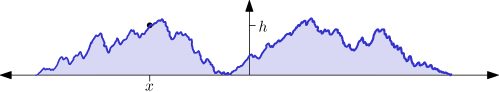
Figure 1. A reflected/absorbed Brownian motion from $(x,h)$ with $x<0$ . It is reflected on the interval $[x,0]$ and absorbed on $\mathbb{R}\setminus[x,0]$. $T(x,h)$ is the area between the curve and the horizontal axis.

The system of independent coalescing Brownian motions starting from every point in $\mathbb{R}^{2}$ is currently known as a “Brownian web” (see [Arr79, FINR02, FINR04, NRS05] and references therein). Since we will need neither the details of the above construction nor the Brownian web in the present work, we will restrict ourselves with a brief overview of some of the important properties of the TSRM and its local time that will be used later in the paper. We refer to [TW98] for proofs and additional details.

$\circ$ Continuity and scaling. The process $t\mapsto\mathfrak{X}(t)$, $t\geq 0$, is almost surely continuous and satisfies the following scaling relation:

(5) $$(\mathfrak{X}(ct))_{t\geq 0}\overset{\text{Law}}{=}(c^{2/3}\mathfrak{X}(t))_{t\geq 0},\qquad\forall c\geq 0.$$

$\circ$ Local times and occupation time formulas. There is a local time process $(\mathfrak{L}(t,x))_{t\geq 0,x\in\mathbb{R}}$ for $\mathfrak{X}$ in the sense that, almost surely, for all $t\geq 0$ the occupation time measure $\mu_{t}$ of $\mathfrak{X}$ on the time interval $[0,t]$ defined by

$$\mu_{t}(A)=\int_{0}^{t}\mathbbm{1}_{\{\mathfrak{X}(s)\in A\}}\,ds,\qquad\text{for all Borel }A\subset\mathbb{R},$$

is absolutely continuous with respect to the Lebesgue measure on the Borel $\sigma$-field with density $\mathfrak{L}(t,\cdot)$. The mapping $t\mapsto\mathfrak{L}(t,\cdot)$ is non-decreasing continuous from $[0,\infty)$ to the space of continuous functions with compact support with topology induced by uniform convergence on compact intervals.

The process $\mathfrak{H}(t)=\mathfrak{L}(t,\mathfrak{X}(t))$, $t\geq 0$, is almost surely continuous and we have the following generalization of the occupation time formula: almost surely, for any bounded, measurable function $\phi:\mathbb{R}\times\mathbb{R}_{+}\to\mathbb{R}$ and any $t\geq 0$,

$$\int_{0}^{t}\phi(\mathfrak{X}(s),\mathfrak{H}(s))\,ds=\int_{\mathbb{R}}\int_{0}^{t}\phi(x,\mathfrak{L}(s,x))d_{s}\mathfrak{L}(s,x)\,dx=\int_{\mathbb{R}}\int_{[0,\mathfrak{L}(t,x))}\phi(x,h)\,dh\,dx.$$

The first equality is an application of [TW98, Theorem 4.2(ii)] with $g(t,x)=\phi(x,\mathfrak{L}(t,x))$ and the second is the change of variables. In fact, we will use a multi-dimensional version of this formula which can be obtained from the above by using Fubini’s Theorem: for any bounded, measurable $f:\mathbb{R}^{k}\times\mathbb{R}^{k}_{+}\to\mathbb{R}$ and any $t_{1},t_{2},\ldots,t_{k}\geq 0$,

(6) $$\int_{\prod_{i=1}^{k}[0,t_{i}]}\phi(\mathfrak{X}(s_{1}),\dots,\mathfrak{X}(s_{k}),\mathfrak{H}(s_{1}),\dots,\mathfrak{H}(s_{k}))\,ds_{1}\ldots ds_{k}\\ =\int_{\mathbb{R}^{k}}\int_{\prod_{i=1}^{k}[0,\mathfrak{L}(t_{i},x_{i}))}\phi(x_{1},\ldots,x_{k},h_{1},\ldots,h_{k})\,dh_{1}\ldots dh_{k}\,dx_{1}\ldots dx_{k}.$$

$\circ$ Ray-Knight curves and their merge and absorption times. For any $(x,h)\in\mathbb{R}\times\mathbb{R}_{+}$ let $\mathfrak{t}_{x,h}$ be the first time when the local time of $\mathfrak{X}$ at $x$ exceeds $h$,

(7) $$\mathfrak{t}_{x,h}=\inf\{t\geq 0:\,\mathfrak{L}(t,x)>h\},$$

and define the local time profile of $\mathfrak{X}$ at time $\mathfrak{t}_{x,h}$ by

(8) $$\Lambda_{x,h}(y)=\mathfrak{L}\left(\mathfrak{t}_{x,h},y\right),\quad y\in\mathbb{R}.$$

We note that $\Lambda_{x,h}(x)=h$ and will refer to $\Lambda_{x,h}(\cdot)$ as a Ray-Knight curve indexed by $(x,h)$.

For $x,x^{\prime}\in\mathbb{R}$ and $h,h^{\prime}\geq 0$ let

$$\mathfrak{m}_{(x,h),(x^{\prime},h^{\prime})}^{+}=\inf\left\{y\geq x\vee x^{\prime}:\Lambda_{x,h}(y)=\Lambda_{x^{\prime},h^{\prime}}(y)\right\},$$

and

$$\mathfrak{m}_{(x,h),(x^{\prime},h^{\prime})}^{-}=\sup\left\{y\leq x\wedge x^{\prime}:\Lambda_{x,h}(y)=\Lambda_{x^{\prime},h^{\prime}}(y)\right\}.$$

Thus, $\mathfrak{m}_{(x,h),(x^{\prime},h^{\prime})}^{+}$ and $\mathfrak{m}_{(x,h),(x^{\prime},h^{\prime})}^{-}$ are the locations right of $x\vee x^{\prime}$ and left of $x\wedge x^{\prime}$, respectively, where the curves $\Lambda_{x,h}$ and $\Lambda_{x^{\prime},h^{\prime}}$ coalesce. They also represent the maximal and minimal points, respectively, that the process $\mathfrak{X}$ reaches between the times $\mathfrak{t}_{x,h}$ and $\mathfrak{t}_{x^{\prime},h^{\prime}}$. Since $\Lambda_{0,0}(y)\equiv 0$, the values $\mathfrak{m}_{(0,0),(x,h)}^{+}=:\mathfrak{m}_{x,h}^{+}$ and $\mathfrak{m}_{(0,0),(x,h)}^{-}=:\mathfrak{m}_{x,h}^{-}$ give the locations to the right of $x\vee 0$ and left of $x\wedge 0$, respectively, where the curve $\Lambda_{x,h}$ is absorbed at zero, and thus are also the maximum and the minimum of the TSRM up to $\mathfrak{t}_{x,h}$ so that we can write

(9) $$\mathfrak{t}_{x,h}=\int_{\mathbb{R}}\Lambda_{x,h}(y)\,dy=\int_{\mathfrak{m}_{x,h}^{-}}^{\mathfrak{m}_{x,h}^{+}}\Lambda_{x,h}(y)\,dy,\qquad\forall(x,h)\in\mathbb{R}\times\mathbb{R}_{+}.$$

$\circ$ Joint Ray-Knight Theorems for the TSRM. For any finite set of points $(x_{1},h_{1}),(x_{2},h_{2}),\ldots,$ $(x_{k},h_{k})\in\mathbb{R}\times[0,\infty)$, the curves $(\Lambda_{x_{i},h_{i}}(\cdot))_{i\leq k}$ are a family of independent coalescing reflected/absorbed Brownian motions. We will need the following more detailed description.

1. Marginal curve distribution. For each $i$ the process $\Lambda_{x_{i},h_{i}}(\cdot)$ is a two-sided reflected/absorbed Brownian motion. To the right of $x_{i}$ the process is a one-dimensional Brownian motion started with initial value $\Lambda_{x_{i},h_{i}}(x_{i})=h_{i}$ which is reflected at 0 on the interval $[x_{i},0]$ if $x_{i}<0$ and absorbed at 0 on $[0\vee x_{i},\infty)$. To the left of $x_{i}$ the process is a one-dimensional Brownian motion (which is independent of the process to the right of $x_{i}$) also started at $h_{i}$, reflected at 0 on the interval $[0,x_{i}]$ if $x_{i}>0$ and absorbed at 0 on the interval $(-\infty,x_{i}\wedge 0]$. See Figure 1.

2. Joint forward curve distribution. For each $i$ let $\Lambda_{x_{i},h_{i}}^{+}(\cdot)$ denote the part of the curve $\Lambda_{x_{i},h_{i}}(\cdot)$ restricted to the interval $[x_{i},\infty)$. Then the joint distribution of the curves $(\Lambda_{x_{i},h_{i}}^{+}(\cdot))_{i\leq k}$ is as follows: the curves evolve as reflected/absorbed Brownian motions (as described above) which are independent until they meet and which coalesce upon their first intersection. See Figure 2.

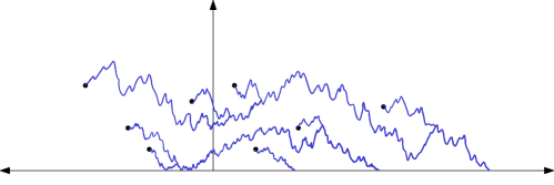
Figure 2. A system of independent coalescing, reflected/absorbed Brownian motions $(\Lambda_{x_{i},h_{i}}^{+}(\cdot))_{i\leq k}$.

Remark 3.

The inverse local times $\mathfrak{t}_{x,h}$ (see (7)) that we use in our paper correspond to $T^{+}(x,h)$ in [TW98]. Many of the results in [TW98] are stated instead in terms of the stopping times $T(x,h)=\inf\{t\geq 0:\,\mathfrak{L}(t,x)=h\}$ for $x\in\mathbb{R}$ and $h>0$. The only difference between $T^{+}(x,h)$ and $T(x,h)$ is that $h\mapsto T(x,h)$ is left continuous while $h\mapsto T^{+}(x,h)$ is right continuous. In particular, for a fixed $(x,h)$ with $h>0$ we have that $T(x,h)=T^{+}(x,h)$, almost surely. The choice of $\mathfrak{t}_{x,h}=T^{+}(x,h)$ is more convenient for our purposes, in part because then the Ray-Knight Theorems in [TW98, Theorem 4.3] are true for all $h\geq 0$ rather than just for $h>0$.

2.2. Discrete Ray-Knight curves and the joint GRKT

Recall the definition of local times (3) and let

$$\tau_{k,m}=\inf\{n\geq 0:L(n,k)>m\},\quad k\in\mathbb{Z},\ m\in\mathbb{Z}_{+},$$

be the time of the $(m+1)$-th visit of the TSAW to $k$. The joint GRKT for the TSAW will describe the convergence of the rescaled local time profile of the random walk at finitely many stopping times $\tau_{k,m}$ with $k$ of order $n$ and $m$ of order $\sqrt{n}$. To this end, for any $(x,h)\in\mathbb{R}\times\mathbb{R}_{+}$ we define the rescaled local times curve $\Lambda_{x,h}^{n}(\cdot)$ at time $\tau_{\lfloor xn\rfloor,\lfloor 2\sigma h\sqrt{n}\rfloor}$ by

(10) $$\Lambda_{x,h}^{n}(y)=\frac{L\left(\tau_{\lfloor xn\rfloor,\lfloor 2\sigma h\sqrt{n}\rfloor},\lfloor yn\rfloor\right)}{2\sigma\sqrt{n}},$$

where $\sigma$ is given by (4). The joint GRKT stated below gives the joint weak convergence of a finite set of curves $\Lambda_{x_{i},h_{i}}^{n}(\cdot)$, $1\leq i\leq N$, together with the locations where these curves coalesce or get absorbed. Hence, we shall need notation for recording this information. For any $k,k^{\prime}\in\mathbb{Z}$ and $m,m^{\prime}\geq 0$ let

$$\mu_{(k,m),(k^{\prime},m^{\prime})}^{+} =\max\left\{X_{i}:\tau_{k,m}\wedge\tau_{k^{\prime},m^{\prime}}\leq i\leq\tau_{k,m}\vee\tau_{k^{\prime},m^{\prime}}\right\}$$

$$=\min\left\{j\geq k\vee k^{\prime}:\mathcal{E}_{\tau_{k,m}}^{+}(j)=\mathcal{E}_{\tau_{k^{\prime},m^{\prime}}}^{+}(j)\right\}$$

and

$$\mu_{(k,m),(k^{\prime},m^{\prime})}^{-} =\min\left\{X_{i}:\tau_{k,m}\wedge\tau_{k^{\prime},m^{\prime}}\leq i\leq\tau_{k,m}\vee\tau_{k^{\prime},m^{\prime}}\right\}$$

$$=\max\left\{j\leq k\wedge k^{\prime}:\mathcal{E}_{\tau_{k,m}}^{-}(j)=\mathcal{E}_{\tau_{k^{\prime},m^{\prime}}}^{-}(j)\right\}$$

be the farthest the random walk ever is to the right or left between the stopping times $\tau_{k,m}$ and $\tau_{k^{\prime},m^{\prime}}$. Note that these random variables differ by at most 1 from the first location to the right of $k\vee k^{\prime}$ or left of $k\wedge k^{\prime}$, respectively, where the local time processes at times $\tau_{k,m}$ and $\tau_{k^{\prime},m^{\prime}}$ are equal. Since $\Lambda^{n}_{0,0}(y)\equiv 0$, the values $\mu^{+}_{(0,0),(k,m)}=:\mu^{+}_{k,m}$ and $\mu^{-}_{(0,0),(k,m)}=:\mu^{-}_{k,m}$ give the locations to the right of $k\vee 0$ and left of $k\wedge 0$, respectively, where the curve $\Lambda^{n}_{k,m}$ is absorbed at zero. These values are also the maximum and the minimum of the TSAW up to time $\tau_{k,m}$.

To lighten the notation, for $x,x^{\prime}\in\mathbb{R}$ and $h,h^{\prime}\in\mathbb{R}_{+}$ we let

(11) $$\tau^{n}_{x,h} =\tau_{\lfloor xn\rfloor,\lfloor 2\sigma h\sqrt{n}\rfloor};$$

(12) $$\mu^{n,\pm}_{x,h} =n^{-1}\mu^{\pm}_{(\lfloor xn\rfloor,\lfloor 2\sigma h\sqrt{n}\rfloor)},\quad\mu^{n,\pm}_{(x,h),(x^{\prime},h^{\prime})}=n^{-1}\mu^{\pm}_{(\lfloor xn\rfloor,\lfloor 2\sigma h\sqrt{n}\rfloor),(\lfloor x^{\prime}n\rfloor,\lfloor 2\sigma h^{\prime}\sqrt{n}\rfloor)}.$$

Theorem 4 (Joint GRKT).

For any $N\in\mathbb{N}$ and any choice of $(x_{i},h_{i})\in\mathbb{R}\times\mathbb{R}_{+}$, $1\leq i\leq N$, the joint distribution (in the natural product topology) of the processes $\Lambda_{x_{i},h_{i}}^{n}(\cdot)$, the rescaled endpoints $\mu^{n,*}_{(x_{i}h_{i})}$, and merging points $\mu^{n,*}_{(x_{i},h_{i}),(x_{j},h_{j})}$, $1\leq i\leq N,\,i<j\leq N,\,*\in\{+,-\}$, converges as $n\to\infty$ to the joint distribution of $\Lambda_{x_{i},h_{i}}(\cdot)$, $\mathfrak{m}^{*}_{x_{i},h_{i}}$, and $\mathfrak{m}^{*}_{(x_{i},h_{i}),(x_{j},h_{j})}$, $1\leq i\leq N,\,i<j\leq N,\,*\in\mathcal{\{}+,-\}$.

For $N=1$ this theorem was proven in [Tót95, Theorem 1]. We state it and discuss a minor difference with our formulation in Section 4. In [TW98] the authors suggested that the methods of [Tót95] can be used to show the joint convergence of the rescaled edge local times to independent coalescing reflected/absorbed Brownian motions, see [TW98, (1.13)]. We show that this is indeed the case. Yet we would like to point out that the generalization from $N=1$ to an arbitrary $N$ is non-trivial and quite technical due to the included convergence of the merge and absorption points. The reader is referred to Section 4 for a proof.

2.3. Consequences of the joint GRKT

We conclude this section with two consequences of Theorem 4 that will be the key tools used in our proof of Theorem 1.

The first one is the weak convergence of the rescaled inverse local times of the TSAW to those of the true self-repelling motion.

Corollary 5.

For any $N\geq 1$ and any choice of $(x_{i},h_{i})\in\mathbb{R}\times\mathbb{R}_{+}$, $1\leq i\leq N$, we have

$$\left(\frac{\tau^{n}_{x_{i},h_{i}}}{2\sigma n^{3/2}}\right)_{i\leq N}\underset{n\to\infty}{\Longrightarrow}\left(\mathfrak{t}_{x_{i},h_{i}}\right)_{i\leq N}.$$

Proof.

Since $\tau_{k,m}+1=\sum_{j\in\mathbb{Z}}L(\tau_{k,m},i)$, we see that

$$\frac{\tau^{n}_{x_{i},h_{i}}}{2\sigma n^{3/2}}+\frac{1}{2\sigma n^{3/2}} =\frac{1}{2\sigma n^{3/2}}\sum_{k\in\mathbb{Z}}L\left(\tau^{n}_{x_{i},h_{i}},k\right)$$

(13) $$\overset{\eqref{dRKpath}}{=}\frac{1}{n}\sum_{k\in\mathbb{Z}}\Lambda^{n}_{x_{i},h_{i}}\left(k/n\right)=\int_{\mathbb{R}}\Lambda^{n}_{x_{i},h_{i}}(y)\,dy=\int_{\mu^{n,-}_{x_{i},h_{i}}}^{\mu^{n,+}_{x_{i},h_{i}}}\Lambda^{n}_{x_{i},h_{i}}(y)\,dy.$$

The statement now follows easily from (9) and Theorem 4. Note that in the application of Theorem 4 we are using both the convergence of the curves $\Lambda^{n}_{x_{i},h_{i}}(\cdot)$ and the endpoints of the curves in order to conclude that the integrals of $\Lambda^{n}_{x_{i},h_{i}}$ converge in distribution to the integrals of $\Lambda_{x_{i},h_{i}}$ as $n\to\infty$. ∎

An immediate consequence of Corollary 5 is convergence of the multi-dimensional Laplace transforms of these rescaled hitting times. That is, for any fixed $k\in\mathbb{N}$, $(x_{i},h_{i})\in\mathbb{R}\times\mathbb{R}_{+}$, and $\lambda_{i}>0$, $i\in\{1,2,\ldots,k\}$, we have

$$\lim_{n\to\infty}E\left[e^{-n^{-3/2}\sum_{i=1}^{k}\lambda_{i}\tau^{n}_{x_{i},h_{i}}}\right]=E\left[e^{-\sum_{i=1}^{k}2\sigma\lambda_{i}\mathfrak{t}_{x_{i},h_{i}}}\right].$$

The above suggests that scaling of the time by $n^{3/2}$ rather than by $n$ might be more natural for the methods we are going to use. To this end, we define for $t\geq 0$

(14) $$\mathcal{X}_{n}(t)=\frac{X_{\lfloor tn^{3/2}\rfloor}}{(2\sigma)^{-2/3}n},\ \ \mathcal{H}_{n}(t)=\frac{L(\lfloor tn^{3/2}\rfloor,X_{\lfloor tn^{3/2}\rfloor})}{(2\sigma)^{2/3}\sqrt{n}},$$

where $\sigma$ is given by (4). At the beginning of the next section we shall briefly argue that the weak convergence of ${\cal D}^{2}$-valued random variables $(\mathcal{X}_{n}(\cdot),\mathcal{H}_{n}(\cdot))$, $n\in\mathbb{N}$, is equivalent to the convergence claimed in Theorem 1.

The second main consequence of Theorem 4 is tightness of the rescaled paths of the TSAW and its local times.

Proposition 6.

The sequence of ${\cal D}^{2}$-valued random variables $(\mathcal{X}_{n},\mathcal{H}_{n})$, $n\in\mathbb{N}$, is tight (with respect to the Skorokhod $J_{1}$ topology on ${\cal D}^{2}$). Moreover, any subsequential limit is concentrated on paths that are continuous.

Proposition 6 will be proved in Section 5 using Theorem 4. Below we will simply give some intuition into the role that the joint GRKT plays in proving tightness.

We first note how the joint GRKT for the TSRM $\mathfrak{X}$ can be used to control the continuity of $\mathfrak{X}$. If there exist times $s,t$ with $|s-t|<\delta$ and $|\mathfrak{X}(t)-\mathfrak{X}(s)|>\varepsilon$, then there must be inverse local times $\mathfrak{t}_{x,h}$ and $\mathfrak{t}_{x^{\prime},h^{\prime}}$ with $|x-x^{\prime}|>\varepsilon$ and

$$\delta>|\mathfrak{t}_{x,h}-\mathfrak{t}_{x^{\prime},h^{\prime}}|=\int_{\mathbb{R}}\left|\Lambda_{x,h}(y)-\Lambda_{x^{\prime},h^{\prime}}(y)\right|\,dy$$

However, since $\Lambda_{x,h}(\cdot)$ and $\Lambda_{x^{\prime},h^{\prime}}$ are independent coalescing reflected/absorbed Brownian motions, it is very unlikely that the curves $\Lambda_{x,h}$ and $\Lambda_{x^{\prime},h^{\prime}}$ can have a small area between them if $x$ and $x^{\prime}$ are far apart (it should be noted that the curves can coalesce only outside of the interval $[x\wedge x^{\prime},x\vee x^{\prime}]$). The same ideas can be applied to the random walk and the corresponding curves $\Lambda^{n}_{x,h}$ which appear in Theorem 4. Combining the tightness of the sequence of the spatial coordinates with properties of the local times we then show the tightness of $({\cal H}_{n})_{n\in\mathbb{N}}$ and complete the proof of Proposition 6.

3. Proof of Theorem 1

In this section, we prove Theorem 1 using the results stated in the previous section. As we remarked above, it suffices to prove the following statement.

Theorem 7.

The sequence of ${\cal D}^{2}$-valued random variables $(\mathcal{X}_{n}(\cdot),\mathcal{H}_{n}(\cdot))$, $n\in\mathbb{N}$, defined in (14) converges weakly as $n\to\infty$ to $(\mathfrak{X}(\cdot),\mathfrak{H}(\cdot))$.

Indeed, let $k_{n}=\lfloor n^{2/3}\rfloor$ and $t_{n}=tn/k^{3/2}_{n}$. Writing

$$\left(\frac{X_{\lfloor tn\rfloor}}{(2\sigma)^{-2/3}n^{2/3}},\frac{L\left(\lfloor tn\rfloor,X_{\lfloor tn\rfloor}\right)}{(2\sigma)^{2/3}n^{1/3}}\right)=\left(\frac{k_{n}}{n^{2/3}}{\cal X}_{k_{n}}(t_{n}),\frac{k_{n}^{1/2}}{n^{1/3}}{\cal H}_{k_{n}}(t_{n})\right)$$

and using the fact that $k_{n}/n^{2/3}\to 1$ and $0\leq t_{n}-t\to 0$ as $n\to\infty$ locally uniformly in $t\geq 0$, we see that for every $T>0$ the Skorokhod distance between the last process and $({\cal X}_{k_{n}}(t),{\cal H}_{k_{n}}(t))$ on the interval $[0,T]$ goes to $0$ as $n\to\infty$. We conclude that Theorem 7 implies Theorem 1.

3.1. Proof of Theorem 7

The first step in the proof of Theorem 7 is to show the convergence of finite dimensional distributions for the processes $(\mathcal{X}_{n}(\cdot),{\cal H}_{n}(\cdot))_{n\in\mathbb{N}}$ sampled not at deterministic times but at independent exponential times. Without loss of generality we expand the probability spaces of the random walk and the process $\mathfrak{X}$ to include the exponential random variables that are also independent of both the TSAW and the process $\mathfrak{X}$.

Theorem 8 (Joint weak limit at independent geometric stopping times).

For any choice of parameters $\lambda_{1},\lambda_{2},\ldots,\lambda_{k}>0$, let $\gamma_{1},\gamma_{2},\ldots,\gamma_{k}$ be independent random variables with $\gamma_{i}\sim\text{Exp}(\lambda_{i})$ that are also independent of both the TSAW and the true self-repelling motion $\mathfrak{X}$. Then,

$$\left(\mathcal{X}_{n}(\gamma_{i}),\mathcal{H}_{n}(\gamma_{i})\right)_{1\leq i\leq k}\ \underset{n\to\infty}{\Longrightarrow}\left(\mathfrak{X}(\gamma_{i}),\mathfrak{H}(\gamma_{i})\right)_{1\leq i\leq k}.$$

Remark 9.

The proof of Theorem 8 is similar to that of [Tót95, Theorem 3]. We note, however, two differences. First, we are able to identify the density of the limiting random vector as that of $(\mathfrak{X},\mathfrak{H})$ stopped at random exponential times (recall that [Tót95] preceded the construction of the TSRM). Secondly, our proof gives a local limit theorem for $(X_{\lfloor\gamma_{i}n^{3/2}\rfloor},H_{\lfloor\gamma_{i}n^{3/2}\rfloor})$ rather than for $X_{\lfloor\gamma_{i}n^{3/2}\rfloor}$. The local limit theorem for $X_{\lfloor\gamma_{i}n^{3/2}\rfloor}$ can also be obtained by providing appropriate uniform tail estimates and an application of the dominated convergence theorem. Since we do not need this result we omit the details. We remark that a proof given in [Tót95] which uses only Fatou’s lemma appears to be incomplete as only a liminf rather than the claimed limit is proved.

Proof.

Let $H_{n}=L(n,X_{n})$ and recall (14). We shall first prove that

(15) $$\begin{split}\lim_{n\to\infty}&n^{3k/2}P\left(X_{\lfloor\gamma_{i}n^{3/2}\rfloor}=\lfloor(2\sigma)^{-2/3}a_{i}n\rfloor,\,H_{\lfloor\gamma_{i}n^{3/2}\rfloor}=\lfloor(2\sigma)^{2/3}h_{i}\sqrt{n}\rfloor+1,\,\forall i\leq k\right)\\ &=E\left[\prod_{i=1}^{k}\lambda_{i}e^{-\lambda_{i}\mathfrak{t}_{a_{i},h_{i}}}\right],\qquad\forall a_{1},a_{2},\ldots,a_{k}\in\mathbb{R},\,\forall h_{1},h_{2},\ldots,h_{k}\geq 0,\end{split}$$

and then show that the right-hand side is the joint density of $\left(\mathfrak{X}(\gamma_{i}),\mathfrak{H}(\gamma_{i})\right)$, $1\leq i\leq k$. Indeed, we can interpret the expression under the limit as a density of a $2k$-dimensional random vector with a piecewise constant density, so that the above convergence of densities by Scheffe’s lemma gives us the weak convergence of this sequence of $2k$-dimensional random vectors to $\left(\mathfrak{X}(\gamma_{i}),\mathfrak{H}(\gamma_{i})\right)$, $1\leq i\leq k$. The statement of the theorem follows by noticing that the random variables $\left(\mathcal{X}_{n}(\gamma_{i}),\mathcal{H}_{n}(\gamma_{i})\right)$, $i\leq k$ can be coupled with joint random variables whose density is given by the left side of (15) in such a way that the maximum difference of any coordinate is $\mathcal{O}(n^{-1/2})$.

To prove (15), note that $\lfloor\gamma_{i}n^{3/2}\rfloor\sim\text{Geo}(1-e^{-\lambda_{i}n^{-3/2}})$ so that by conditioning on the values of these independent geometric random variables we get

$$P\left(X_{\lfloor\gamma_{i}n^{3/2}\rfloor}=\left\lfloor\tfrac{a_{i}n}{(2\sigma)^{2/3}}\right\rfloor,H_{\lfloor\gamma_{i}n^{3/2}\rfloor}=\lfloor(2\sigma)^{2/3}h_{i}\sqrt{n}\rfloor+1,\,\forall i\leq k\right)$$

$$=\sum_{j_{1},j_{2},\ldots,j_{k}\geq 0}\left(\prod_{i=1}^{k}(1-e^{-\lambda_{i}n^{-3/2}})\,e^{-\lambda_{i}n^{-3/2}j_{i}}\right)$$

$$\makebox[133.72786pt]{\ }\times P\left(X_{j_{i}}=\left\lfloor\tfrac{a_{i}n}{(2\sigma)^{2/3}}\right\rfloor,H_{j_{i}}=\lfloor(2\sigma)^{2/3}h_{i}\sqrt{n}\rfloor+1,\,\forall i\leq k\right)$$

$$=\sum_{j_{1},\ldots,j_{k}\geq 0}\left(\prod_{i=1}^{k}(1-e^{-\lambda_{i}n^{-3/2}})\,e^{-\lambda_{i}n^{-3/2}j_{i}}\right)P\left(\tau_{\lfloor(2\sigma)^{-2/3}a_{i}n\rfloor,\lfloor(2\sigma)^{2/3}h_{i}\sqrt{n}\rfloor}=j_{i},\,\forall i\leq k\right)$$

$$=\prod_{i=1}^{k}(1-e^{-\lambda_{i}n^{-3/2}})E\left[\prod_{i=1}^{k}\exp\left\{-\lambda_{i}n^{-3/2}\tau_{\lfloor(2\sigma)^{-2/3}a_{i}n\rfloor,\lfloor(2\sigma)^{2/3}h_{i}\sqrt{n}\rfloor}\right\}\right].$$

Therefore, it follows from Corollary 5 that

$$\lim_{n\to\infty}n^{3k/2}P\left(X_{\lfloor\gamma_{i}n^{3/2}\rfloor}=\lfloor(2\sigma)^{-2/3}a_{i}n\rfloor,\,H_{\lfloor\gamma_{i}n^{3/2}\rfloor}=\lfloor(2\sigma)^{2/3}h_{i}\sqrt{n}\rfloor+1,\,\forall i\leq k\right)$$

$$=\lim_{n\to\infty}\left(\prod_{i=1}^{k}n^{3/2}(1-e^{-\lambda_{i}n^{-3/2}})\right)E\left[\prod_{i=1}^{k}\exp\left\{-\lambda_{i}n^{-3/2}\tau_{\lfloor(2\sigma)^{-2/3}a_{i}n\rfloor,\lfloor(2\sigma)^{2/3}h_{i}\sqrt{n}\rfloor}\right\}\right]$$

$$=\left(\prod_{i=1}^{k}\lambda_{i}\right)E\left[\prod_{i=1}^{k}\exp\left\{-2\sigma\lambda_{i}\mathfrak{t}_{(2\sigma)^{-2/3}a_{i},(2\sigma)^{-1/3}h_{i}}\right\}\right]=\left(\prod_{i=1}^{k}\lambda_{i}\right)E\left[\prod_{i=1}^{k}e^{-\lambda_{i}\mathfrak{t}_{a_{i},h_{i}}}\right],$$

where in the last equality we used that $(\mathfrak{t}_{ca_{i},\sqrt{c}h_{i}})_{i\leq k}\overset{\text{Law}}{=}(c^{3/2}\,\mathfrak{t}_{a_{i},h_{i}})_{i\leq k}$ for any $c>0$, which follows from (9), the fact that the curves $(\Lambda_{a_{i},h_{i}}(\cdot))_{i\leq k}$ are independent coalescing reflected/absorbed Brownian motions, and then the scaling property of Brownian motion.

We have completed the proof of (15), and now it remains to show that $((a_{1},h_{1}),\ldots,(a_{k},h_{k}))\mapsto E\left[\prod_{i=1}^{k}\lambda_{i}e^{-\lambda_{i}\mathfrak{t}_{a_{i},h_{i}}}\right]$ is the joint density for $\left(\mathfrak{X}(\gamma_{i}),\mathfrak{H}(\gamma_{i})\right)$, $1\leq i\leq k$. To this end, fix a bounded continuous function $\phi:\mathbb{R}^{k}\times\mathbb{R}_{+}^{k}\to\mathbb{R}$ and note that (using the notation $\mathbf{a}=(a_{1},\ldots,a_{k})$, $\mathbf{h}=(h_{1},\ldots,h_{k})$, $\mathbf{da}=da_{1}\cdots da_{k}$ and $\mathbf{dh}=dh_{1}\cdots dh_{k}$)

$$\int_{\mathbb{R}^{k}}\int_{\mathbb{R}_{+}^{k}}\phi(\mathbf{a},\mathbf{h})E\left[\prod_{i=1}^{k}\lambda_{i}e^{-\lambda_{i}\mathfrak{t}_{a_{i},h_{i}}}\right]\mathbf{dh}\,\mathbf{da}$$

$$=\left(\prod_{i=1}^{k}\lambda_{i}\right)\int_{\mathbb{R}^{k}}\int_{\mathbb{R}_{+}^{k}}\phi(\mathbf{a},\mathbf{h})P\left(\gamma_{i}>\mathfrak{t}_{a_{i},h_{i}},\,\forall i\leq k\right)\mathbf{dh}\,\mathbf{da}$$

$$=\left(\prod_{i=1}^{k}\lambda_{i}\right)\int_{\mathbb{R}^{k}}\int_{\mathbb{R}_{+}^{k}}\phi(\mathbf{a},\mathbf{h})P\left(\mathfrak{L}(\gamma_{i},a_{i})>h_{i},\,\forall i\leq k\right)\mathbf{dh}\,\mathbf{da}$$

$$=\left(\prod_{i=1}^{k}\lambda_{i}\right)\int_{\mathbb{R}^{k}}\int_{\mathbb{R}_{+}^{k}}\int_{\mathbb{R}_{+}^{k}}\left(\prod_{i=1}^{k}\lambda_{i}e^{-\lambda_{i}s_{i}}\right)\phi(\mathbf{a},\mathbf{h})P\left(\mathfrak{L}(s_{i},a_{i})>h_{i},\,\forall i\leq k\right)\mathbf{ds}\,\mathbf{dh}\,\mathbf{da}$$

$$=\int_{\mathbb{R}_{+}^{k}}\left(\prod_{i=1}^{k}\lambda_{i}^{2}e^{-\lambda_{i}s_{i}}\right)E\left[\int_{\mathbb{R}^{k}}\int_{\mathbb{R}_{+}^{k}}\phi(\mathbf{a},\mathbf{h})\mathbbm{1}_{\{h_{i}<\mathfrak{L}(s_{i},a_{i}),\,\forall i\leq k\}}\,\mathbf{dh}\,\mathbf{da}\right]\mathbf{ds}$$

$$=\int_{\mathbb{R}_{+}^{k}}\left(\prod_{i=1}^{k}\lambda_{i}^{2}e^{-\lambda_{i}s_{i}}\right)E\left[\int_{\mathbb{R}^{k}}\int_{\prod_{i=1}^{k}[0,\mathfrak{L}(s_{i},a_{i}))}\phi(\mathbf{a},\mathbf{h})\,\mathbf{dh}\,\mathbf{da}\right]\mathbf{ds}.$$

By the generalization of the occupation time formula, see (6),

$$\int_{\mathbb{R}^{k}}\int_{\prod_{i=1}^{k}[0,\mathfrak{L}(s_{i},a_{i}))}\phi(\mathbf{a},\mathbf{h})\,\mathbf{dh}\,\mathbf{da}=\int_{\prod_{i=1}^{k}[0,s_{i}]}\phi\left(\mathfrak{X}(t_{1}),\ldots,\mathfrak{X}(t_{k}),\mathfrak{H}(t_{1}),\ldots,\mathfrak{H}(t_{k})\right)\,\mathbf{dt}.$$

Hence,

$$\int_{\mathbb{R}^{k}}\int_{\mathbb{R}_{+}^{k}}\phi(\mathbf{a},\mathbf{h})E\left[\prod_{i=1}^{k}\lambda_{i}e^{-\lambda_{i}\mathfrak{t}_{a_{i},h_{i}}}\right]\mathbf{dh}\,\mathbf{da}$$

$$=\int_{\mathbb{R}_{+}^{k}}\left(\prod_{i=1}^{k}\lambda_{i}^{2}e^{-\lambda_{i}s_{i}}\right)E\left[\int_{\prod_{i=1}^{k}[0,s_{i}]}\phi\left(\mathfrak{X}(t_{1}),\ldots,\mathfrak{X}(t_{k}),\mathfrak{H}(t_{1}),\ldots,\mathfrak{H}(t_{k})\right)\,\mathbf{dt}\right]\,\mathbf{ds}$$

$$=E\left[\int_{\mathbb{R}_{+}^{k}}\phi\left(\mathfrak{X}(t_{1}),\ldots,\mathfrak{X}(t_{k}),\mathfrak{H}(t_{1}),\ldots,\mathfrak{H}(t_{k})\right)\left(\prod_{i=1}^{k}\int_{t_{i}}^{\infty}\lambda_{i}^{2}e^{-\lambda_{i}s_{i}}\,ds_{i}\right)\mathbf{dt}\right]$$

$$=E\left[\int_{\mathbb{R}_{+}^{k}}\phi\left(\mathfrak{X}(t_{1}),\ldots,\mathfrak{X}(t_{k}),\mathfrak{H}(t_{1}),\ldots,\mathfrak{H}(t_{k})\right)\left(\prod_{i=1}^{k}\lambda_{i}e^{-\lambda_{i}t_{i}}\right)\mathbf{dt}\right]$$

$$=E\left[\phi\left(\mathfrak{X}(\gamma_{1}),\ldots,\mathfrak{X}(\gamma_{k}),\mathfrak{H}(\gamma_{1}),\ldots,\mathfrak{H}(\gamma_{k})\right)\right].$$

This completes the proof of the theorem. ∎

We are now ready to prove Theorem 7.

Proof of Theorem 7.

Suppose that $(\mathcal{X}_{n_{j}}(\cdot),\mathcal{H}_{n_{j}}(\cdot))\underset{j\to\infty}{\Longrightarrow}(Y(\cdot),Z(\cdot))$ along a subsequence $(n_{j})_{j\geq 1}$. By Proposition 6 the process $(Y(\cdot),Z(\cdot))$ must be continuous, and it will be enough to show that $(Y(\cdot),Z(\cdot))$ has the same finite dimensional distributions as $(\mathfrak{X}(\cdot),\mathfrak{H}(\cdot))$. To this end, note that it follows from Theorem 8 and the convergence assumption that for any bounded continuous function $\phi:\mathbb{R}^{k}\times\mathbb{R}_{+}^{k}\to\mathbb{R}$, any $\lambda_{1},\lambda_{2},\ldots,\lambda_{k}>0$, and independent random variables $\gamma_{1},\gamma_{2},\ldots,\gamma_{k}$ with $\gamma_{i}\sim\text{Exp}(\lambda_{i})$, $1\leq i\leq k$, which are also independent from $(Y(\cdot),Z(\cdot))$ and $(\mathfrak{X}(\cdot),\mathfrak{H}(\cdot))$,

$$E\left[\phi\left(Y(\gamma_{1}),\ldots,Y(\gamma_{k}),Z(\gamma_{1}),\ldots,Z(\gamma_{k})\right)\right]=E\left[\phi\left(\mathfrak{X}(\gamma_{1}),\ldots,\mathfrak{X}(\gamma_{k}),\mathfrak{H}(\gamma_{1}),\ldots,\mathfrak{H}(\gamma_{k})\right)\right],$$

or, equivalently, $\forall\lambda_{1},\lambda_{2},\ldots,\lambda_{k}>0$

$$\int_{[0,\infty)^{k}}\left(\prod_{i=1}^{k}\lambda_{i}e^{-\lambda_{i}t_{i}}\right)E\left[\phi\left(\mathfrak{X}(t_{1}),\ldots,\mathfrak{X}(t_{k}),\mathfrak{H}(t_{1}),\ldots,\mathfrak{H}(t_{k})\right)\right]\,dt_{1}\ldots dt_{k}$$

$$\qquad=\int_{[0,\infty)^{k}}\left(\prod_{i=1}^{k}\lambda_{i}e^{-\lambda_{i}t_{i}}\right)E\left[\phi\left(Y(t_{1}),\ldots,Y(t_{k}),Z(t_{1}),\ldots,Z(t_{k})\right)\right]\,dt_{1}\ldots dt_{k}.$$

That is, for any bounded continuous function $\phi$, the functions

$$(t_{1},\ldots,t_{k}) \mapsto E\left[\phi\left(\mathfrak{X}(t_{1}),\ldots,\mathfrak{X}(t_{k}),\mathfrak{H}(t_{1}),\ldots,\mathfrak{H}(t_{k})\right)\right]\quad\text{and}$$

$$(t_{1},\ldots,t_{k}) \mapsto E\left[\phi\left(Y(t_{1}),\ldots,Y(t_{k}),Z(t_{1}),\ldots,Z(t_{k})\right)\right]$$

(which are also bounded and continuous) have the same $k$-dimensional Laplace transforms and are thus equal for all $(t_{1},\ldots,t_{k})\in[0,\infty)^{k}$. This is enough to conclude that $(Y(\cdot),Z(\cdot))$ has the same finite dimensional distributions as $(\mathfrak{X}(\cdot),\mathfrak{H}(\cdot))$, and since this is true for any subsequential limit $(Y(\cdot),Z(\cdot))$ of $(\mathcal{X}_{n}(\cdot),\mathcal{H}_{n}(\cdot))$ we can conclude that indeed $(\mathcal{X}_{n}(\cdot),\mathcal{H}_{n}(\cdot))\underset{n\to\infty}{\Longrightarrow}(\mathfrak{X}(\cdot),\mathfrak{H}(\cdot))$. ∎

4. Joint generalized Ray-Knight Theorems (GRKTs)

In this section we will prove Theorem 4. Before beginning the proof, we note that this is essentially a “multi-curve” extension of the Ray-Knight type theorems proved for the TSAW in [Tót95, Theorem 1] and a strengthening of the joint GRKT stated but not proved in [TW98].

We stated the joint GRKT for the rescaled local time processes so that it is convenient for our applications. In fact, it is the directed edge local times processes ${\cal E}^{+}_{\tau_{k,m}}(\ell),\ \ell\geq k$, that we are going to use to prove the joint GRKT, since they are Markov chains whose probability to jump from $n$ to $n+x$, $x\in\mathbb{Z}$, is very close for $n\gg 1$ to a symmetric distribution $(\pi(x))_{x\in\mathbb{Z}}$ with Gaussian tails, more precisely, $\pi(x)=C\lambda^{x^{2}}$ for some $C>0$. The transition probabilities of these Markov chains can be conveniently written in terms of generalized Polya’s urn processes for which $\pi$ is the invariant distribution. The parameter $\sigma$ in (4) is simply the standard deviation of $\pi$. We refer the reader to Appendix A for a careful account of the above mentioned connections and related facts.

The following proposition is all we need from Appendix A to proceed with the proof of Theorem 4. It says that if we consider the joint distribution of the processes $\left(\mathcal{E}^{+}_{\tau_{k,m_{1}}},\mathcal{E}^{+}_{\tau_{k,m_{2}}},\ldots,\mathcal{E}^{+}_{\tau_{k,m_{N}}}\right)$, then as long as the processes remain far apart, their increments are approximately distributed like the i.i.d. copies from distribution $\pi$. The exponential bound on the total variation distance given below will ensure that the coupling of the increments of these processes to the i.i.d. copies of $\pi$ will not break down for the required length of time with probability tending to 1.

Proposition 10.

There are constants $C_{2},C_{3}>0$ such that the following holds. For any fixed $k\in\mathbb{Z}$, $0\leq m_{1}<m_{2}<\cdots<m_{N}$, $\ell\neq 0$ and any $0\leq n_{1}<n_{2}<\cdots<n_{N}$ (if $\ell>0$ then we need $n_{1}>0$) we have

$$\sum_{k_{1},k_{2},\ldots,k_{N}\in\mathbb{Z}}\left|P\left(\mathcal{E}^{+}_{\tau_{k,m_{i}}}(\ell)=n_{i}+k_{i},\,i\leq N\mid\mathcal{E}^{+}_{\tau_{k,m_{i}}}(\ell-1)=n_{i},\,i\leq N\right)-\prod_{i=1}^{N}\pi(k_{i})\right|$$

$$\qquad\leq C_{3}\sum_{i=1}^{N}e^{-C_{2}(n_{i}-n_{i-1})}.$$

We first note that Theorem 4 holds for a single curve, that is, for $N=1$.

Theorem 11 (Theorem 1 in [Tót95]).

For any fixed $(x,h)\in\mathbb{R}\times[0,\infty)$, the joint distribution of $\left(\Lambda^{n}_{x,h}(\cdot),\mu^{n,-}_{x,h},\mu^{n,+}_{x,h}\right)$ converges as $n\to\infty$ to the distribution of $(\Lambda_{x,h}(\cdot),\mathfrak{m}^{-}_{x,h},\mathfrak{m}^{+}_{x,h})$.

Theorem 11 is somewhat different from [Tót95, Theorem 1], so we will outline how the result stated follows from [Tót95, Theorem 1]. First of all, since

(16) $$L(n,k)=\mathcal{E}_{n}^{+}(k)+\mathcal{E}_{n}^{+}(k-1)-\mathbbm{1}_{\{X_{0}<k<X_{n}\}}+\mathbbm{1}_{\{X_{n}\leq k\leq X_{0}\}},$$

it’s enough to prove the convergence for directed edge local times, i.e., it suffices to show that

(17) $$\left(\mathcal{E}^{+}_{\tau^{n}_{x,h}}(\lfloor\boldsymbol{\cdot}\,n\rfloor)/(\sigma\sqrt{n}),\mu^{n,-}_{x,h},\mu^{n,+}_{x,h}\right)\underset{n\to\infty}{\Longrightarrow}(\Lambda_{x,h}(\cdot),\mathfrak{m}^{-}_{x,h},\mathfrak{m}^{+}_{x,h}).$$

Note that we divide by $\sigma$ instead of $2\sigma$ (compare with (10)) to account for using directed edge local times. The remaining difference with the process in [Tót95] is that instead of the times $\tau_{k,m}$, [Tót95] uses the times $T^{*}_{k,m}$ of the $(m+1)$-th visit to $k$ from $k+1$ (or from $k-1$). However, this difference affects only the starting point of the Markov chains of directed edges, $\mathcal{E}^{+}_{\tau^{n}_{x,h}}(\cdot)$ or $\mathcal{E}^{+}_{T^{*}_{\lfloor xn\rfloor,\lfloor\sigma h\sqrt{n}\rfloor}}(\cdot)$, to the left and right of $\lfloor xn\rfloor$. Moreover, at the stopping time $\tau^{n}_{x,h}=\tau_{\lfloor xn\rfloor,\lfloor 2\sigma h\sqrt{n}\rfloor}$ the walk will have made approximately half of its steps to $\lfloor xn\rfloor$ from the right and half from the left in the sense that

(18) $$\lim_{n\to\infty}\mathcal{E}^{+}_{\tau^{n}_{x,h}}(\lfloor xn\rfloor)/\sqrt{n}=\sigma h,\qquad P\text{-a.s.}$$

while the definition of $T^{*}_{k,m}$ and of the directed edge local times imply that$\mathcal{E}^{+}_{T^{*}_{\lfloor xn\rfloor,\lfloor\sigma h\sqrt{n}\rfloor}}(\lfloor xn\rfloor)=\lfloor\sigma h\sqrt{n}\rfloor+\mathbbm{1}_{\{x\geq 0\}}$. Thus, there is essentially no difference between the processes in (17) and in [Tót95, Theorem 1].

The local time curve $\Lambda^{n}_{x,h}(\cdot)$ for the random walk and the corresponding local time curve $\Lambda_{x,h}(\cdot)$ for the TSRM consist of a “forward” and “backward” curve. For convenience of notation we will use $\Lambda^{n,+}_{x,h}(\cdot)$ and $\Lambda^{n,-}_{x,h}$ to denote the process $\Lambda^{n}_{x,h}(\cdot)$ restricted to $[x,\infty)$ and $(-\infty,x]$, respectively. Similarly, we will let $\Lambda^{+}_{x,h}(\cdot)$ and $\Lambda^{-}_{x,h}(\cdot)$ denote the process $\Lambda_{x,h}(\cdot)$ restricted to $[x,\infty)$ and $(-\infty,x]$, respectively. For a fixed $(x,h)$, the forward and backward discrete curves $\Lambda^{n,+}_{x,h}$ and $\Lambda^{n,-}_{x,h}$ are asymptotically independent. Indeed, since the directed edge local times to the right and left, respectively, are both Markov chains, the dependence is only through the initial conditions, but as noted above the initial conditions of the forward and backward curves are deterministic in the limit (see (18)). Therefore, Theorem 11 can be proved by handling the forward and backward curves separately. That is, we can prove Theorem 11 by proving that $(\Lambda^{n,+}_{x,h}(\cdot),\mu_{x,h}^{n,+})\Rightarrow(\Lambda^{+}_{x,h}(\cdot),\mathfrak{m}_{x,h}^{+})$ and $(\Lambda^{n,-}_{x,h}(\cdot),\mu_{x,h}^{n,-})\Rightarrow(\Lambda^{-}_{x,h}(\cdot),\mathfrak{m}_{x,h}^{-})$.

However, to prove the joint GRKT, Theorem 4, a difficulty arises trying to handle the forward and backward curves for different space-local time starting points. More precisely, given two points $(x_{1},h_{1})$ and $(x_{2},h_{2})$, if $x_{1}<x_{2}$ then it is not too difficult to study the joint distribution of the forward curves $(\Lambda^{n,+}_{x_{1},h_{1}}(\cdot),\Lambda^{n,+}_{x_{2},h_{2}}(\cdot))$ or of the backward curves $(\Lambda^{n,-}_{x_{1},h_{1}}(\cdot),\Lambda^{n,-}_{x_{2},h_{2}}(\cdot))$, but the joint distribution of one forward curve and another backward curve $(\Lambda^{n,+}_{x_{1},h_{1}}(\cdot),\Lambda^{n,-}_{x_{2},h_{2}}(\cdot))$ turns out to be much more difficult to study (and the complication grows as the number of curves $N$ grows). Thankfully, as we will see below, it will be enough to only consider the joint distributions of the forward curves (or the backward curves) alone. The following result gives forward joint GRKT that will be needed. It can be equivalently stated for the backward curves.

Theorem 12 (Joint forward GRKT).

For any $N\in\mathbb{N}$ and any choice of $(x_{i},h_{i})\in\mathbb{R}\times\mathbb{R}_{+}$, $1\leq i\leq N$, the joint distribution of the processes $\Lambda^{n,+}_{x_{i},h_{i}}(\cdot)$, the rescaled endpoints $\mu^{n,+}_{(x_{i}h_{i})}$, and merging points $\mu^{n,+}_{(x_{i},h_{i}),(x_{j},h_{j})}$, $1\leq i\leq N,\,i<j\leq N$, converges as $n\to\infty$ to the joint distribution of $\Lambda^{+}_{x_{i},h_{i}}(\cdot)$, $\mathfrak{m}^{+}_{x_{i},h_{i}}$, and $\mathfrak{m}^{+}_{(x_{i},h_{i}),(x_{j},h_{j})}$, $1\leq i\leq N,\,i<j\leq N$.

Proof.

Due to the relationship between local times of directed edges and local times of sites in (16), it suffices to prove a corresponding joint diffusion limit for directed edge local times. Moreover, by the Markov property there is no loss of generality in assuming that $x_{i}=x$ for all $i$. Details of the proof depend on the sign of $x$ but the difference between the three cases ($x<0,\ x=0,\ x>0$) is very minimal. For that reason, we shall only consider the case $x<0$, in which we have reflection on $[x,0)$ and absorption on $[0,\infty)$. The other two cases have no reflection interval and are simpler.

The proof proceeds by induction on $N$. The case $N=1$ is contained in Theorem 11. See also (17) and discussion below it.

We shall first treat the case $N=2$ in detail. Fix $x<0$, $\varepsilon\in(0,1/100)$, and $0\leq h_{1}<h_{2}$. We start by lining up several facts about two sequences of rescaled reflected coalescing random walks with independent integer-valued increments $\zeta_{i}(j),\ j\in\mathbb{N},\ i=1,2$, with mean $0$, variance $\sigma^{2}\in(0,\infty)$, and a finite third moment. For $i=1,2$ let

$$\lim_{n\to\infty}Y^{n}_{i}(0)=h_{i}\ \text{a.s},\quad Y^{n}_{i}\left(\frac{j}{n}\right)=\left|Y^{n}_{i}\left(\frac{j-1}{n}\right)+\frac{\zeta_{i}(j)}{\sigma\sqrt{n}}\right|,\quad j\geq 1.$$

At each step we first connect $Y^{n}_{i}\left(\frac{j-1}{n}\right)$ and $Y^{n}_{i}\left(\frac{j-1}{n}\right)+\frac{\zeta_{i}(j)}{\sigma\sqrt{n}}$ and then reflect at $0$ if the second point is negative. We get a continuous piecewise linear curve $Y^{n}_{i}(y),\ y\geq 0$, which hits $0$ in the interval $((j-1)/n,j/n)$ if the expression inside the absolute value above is negative. We also define $\widetilde{Y}^{n}_{2}$, to be the walk which starts from $Y^{n}_{2}(0)-\lfloor n^{\varepsilon}\rfloor/(\sigma\sqrt{n})$ and uses the same increments as $Y^{n}_{2}$. Note that $\widetilde{Y}^{n}_{2}\left(\frac{j}{n}\right)=Y^{n}_{2}\left(\frac{j}{n}\right)-\lfloor n^{\varepsilon}\rfloor/(\sigma\sqrt{n})$ up to (not including) the first time the right hand side falls below $0$. We produce $\widetilde{Y}^{n}_{2}(y),\ y\geq 0$, by the same kind of linear interpolation as above and define the hitting times of $0$ after time $|x|$ and the crossing time of $Y^{n}_{1}$ and $\widetilde{Y}^{n}_{2}$ respectively as follows:

$$\nu^{n}_{1}=\inf\{y\geq|x|:Y^{n}_{1}(y)=0\},\ \ \widetilde{\nu}^{n}_{2}=\inf\{y\geq|x|:\widetilde{Y}^{n}_{2}(y)=0\},$$

$$\widetilde{c}^{n}_{1,2}=\inf\{y\geq 0:\widetilde{Y}^{n}_{2}(y)=Y^{n}_{1}(y)\}\ \left(=\inf\{y\geq 0:Y^{n}_{2}(y)-Y^{n}_{1}(y)=\lfloor n^{\varepsilon}\rfloor/(\sigma\sqrt{n})\}\right).$$

• By independence of $Y^{n}_{1}(\cdot)$ and $\widetilde{Y}^{n}_{2}(\cdot)$, convergence of one-dimensional processes (see [NP21]), and the continuous mapping theorem,

  $$(Y^{n}_{1}(\cdot),\widetilde{Y}^{n}_{2}(\cdot),\nu^{n}_{1},\widetilde{\nu}^{n}_{2},\widetilde{c}^{n}_{1,2})\Longrightarrow(|W_{1}(\cdot)|,|W_{2}(\cdot)|,\nu_{1},\nu_{2},c_{1,2})\quad\text{ as $n\to\infty$},$$

  where the independent Brownian motions $W_{1}(\cdot)$ and $W_{2}(\cdot)$ start at $h_{1}$ and $h_{2}$ respectively and the last three stopping times are defined in the same way as for $Y^{n}_{1}(\cdot)$ and $\widetilde{Y}^{n}_{2}(\cdot)$. The continuous mapping theorem is applicable, since the set of discontinuities of the last three functions on the path space of a standard two dimensional Brownian motion has measure $0$.

• We define a mapping $\phi$ which takes a pair of paths $(f_{1},f_{2})\in C([0,\infty))^{2},\ f_{1},f_{2}\geq 0$, $f_{1}(0)\leq f_{2}(0)$, and returns a pair of coalescing paths $\phi(f_{1},f_{2})$ as follows. Let $c(f_{1},f_{2}):=\inf\{y\geq 0:f_{1}(y)=f_{2}(y)\}\in[0,\infty]$ and $\nu_{0}(f_{i})=\inf\{y\geq|x|:f_{i}(y)=0\}\in[|x|,\infty]$. We shall refer to $\nu_{0}$ as a “marked time”. Set

  $$\phi(f_{1},f_{2})(y):=\begin{cases}(f_{1}(y),f_{2}(y)),&\text{if }y\leq c(f_{1},f_{2});\\ (f_{1}(y),f_{1}(y)),&\text{if }y>c(f_{1},f_{2})\ \text{and }c(f_{1},f_{2})\leq\nu_{0}(f_{1});\\ (f_{2}(y),f_{2}(y)),&\text{if }y>c(f_{1},f_{2})\ \text{and }c(f_{1},f_{2})>\nu_{0}(f_{1}).\end{cases}$$

  In words, at the time when the two paths meet we keep only the lower path if they meet before or at the marked time of the lower path and we keep only the upper path if they meet after the marked time of the lower path. This mapping is a.s. continuous for the pair of independent Brownian motions. Hence, just as above, we can conclude the convergence of a pair of rescaled coalescing reflected random walks together with their marked and coalescence times to a pair of coalescing reflected Brownian motions together with their marked and coalescence times.

From now on we assume that $\zeta_{i}(j)\sim\pi$, $i=1,2$, $j\in\mathbb{N}$. Set

(19) $$S^{n}_{i}(j)=\mathcal{E}^{+}_{\tau^{n}_{x,h_{i}}}(j+\lfloor xn\rfloor),\ j\geq 0;\quad W^{n}_{i}(y)=\frac{S^{n}_{i}(yn)}{\sigma\sqrt{n}},\quad yn\in\mathbb{N}_{0},\quad i=1,2,$$

and linearly interpolated in between so that $W^{n}_{i}\in C([0,\infty))$. For convenience we set $S^{n}_{0}(j)=0$ for all $j\geq 0$. Note that $W^{n}_{i}(0)\to h_{i}$, $i=1,2$, a.s. as $n\to\infty$, see (18).

Recall that $\varepsilon\in(0,1/100)$ and define

$$\omega^{n,4\varepsilon}_{i}=\min\{j\geq\lfloor|x|n\rfloor:S^{n}_{i}(j)\leq n^{4\varepsilon}\},\ \ i=1,2;\quad\omega^{n,\varepsilon}_{1,2}=\min\{j\geq 0:S^{n}_{2}(j)-S^{n}_{1}(j)\leq n^{\varepsilon}\}.$$

We consider the pair $(S^{n}_{1},S^{n}_{2})$ and enlarge the probability space as necessary to construct a pair of crossing marked and reflected Markov chains $(R^{n}_{1},\widetilde{R}^{n}_{2})$ as follows. Let $R^{n}_{1}(0)=S^{n}_{1}(0)$ and $\widetilde{R}^{n}_{2}(0)=S^{n}_{2}(0)-\lfloor n^{\varepsilon}\rfloor$.

Up until $\omega^{n,\varepsilon}_{1,2}\wedge\omega^{n,4\varepsilon}_{1}$ we set $R^{n}_{1}(j)=S^{n}_{1}(j)$, couple the increments of $S^{n}_{2}$ with independent increments $\zeta_{2}(j)$ at each step $j$, and set $\widetilde{R}^{n}_{2}(j)=\widetilde{R}^{n}_{2}(0)+\sum_{k=1}^{j}\zeta_{2}(j)$. Given the initial data, the coordinate processes of $(R^{n}_{1},\widetilde{R}^{n}_{2})$ are independent, and $(R^{n}_{1}(j),\widetilde{R}^{n}_{2}(j))=(S^{n}_{1}(j),S^{n}_{2}(j)-\lfloor n^{\varepsilon}\rfloor)$ for $j<\omega^{n,\varepsilon}_{1,2}\wedge\omega^{n,4\varepsilon}_{1}$, provided that the coupling does not break down.

1. If $\omega^{n,\varepsilon}_{1,2}<\omega^{n,4\varepsilon}_{1}$ then

   1. at time $\omega^{n,\varepsilon}_{1,2}$ we decouple $\widetilde{R}^{n}_{2}$ from $S^{n}_{2}$ and simply let $\widetilde{R}^{n}_{2}$ use increments $\zeta_{2}(j)$, i.e., $\widetilde{R}^{n}_{2}(j)=|\widetilde{R}^{n}_{2}(j-1)+\zeta_{2}(j)|$ for all $j>\omega^{n,\varepsilon}_{1,2}$;

   2. $R^{n}_{1}$ continues to follow $S^{n}_{1}$ up to time $\omega^{n,4\varepsilon}_{1}$, after which it uses independent increments $\zeta_{1}(\cdot)$ and follows a reflected marked random walk.

2. If $\omega^{n,\varepsilon}_{1,2}\geq\omega^{n,4\varepsilon}_{1}$ then

   1. at time $\omega^{n,4\varepsilon}_{1}$ we decouple $R^{n}_{1}$ from $S^{n}_{1}$, $R^{n}_{1}$ continues to use independent increments $\zeta_{1}(\cdot)$ and follows a reflected marked random walk;

   2. we continue to couple the increments of $\widetilde{R}^{n}_{2}$ and $S^{n}_{2}$ up to time $\omega^{n,4\varepsilon}_{2}$, starting from which we let $\widetilde{R}^{n}_{2}$ use increments $\zeta_{2}(\cdot)$ and continue as a reflected marked random walk.

We agree that if any of the couplings above breaks down before the specified decoupling time, we shall just use the corresponding independent $\pi$-distributed increments for the rest of the time. Since a single curve gets absorbed within $n^{1+\varepsilon}$ units of time with probability tending to 1, Lemma 24 implies that the above couplings will not break down before the specified decoupling time with probability tending to 1 as $n\to\infty$.

Diffusively rescaling the process $(R^{n}_{1},\widetilde{R}^{n}_{2})$ and “connecting the dots” in the same way as before we get a sequence of pairs of independent reflected marked processes which converge in distribution together with their rescaled marked and crossing times to a pair of independent marked reflected Brownian motions and their marked and crossing times. Indeed, by the result for $N=1$ and fact (I), each sequence of the rescaled coordinate processes together with their rescaled marked times converges to a reflected Brownian motion and its marked time. Since the coordinate processes are independent, the claimed convergence follows. By (II), we get the convergence of rescaled marked coalescing reflected processes $(R^{n}_{1},\widetilde{R}^{n}_{2})$ and sequences of their rescaled marked and coalescence times to a pair of coalescing reflected Brownian motions together with their marked and coalescence times.

Our next task is to sort out the marked and coalescence times and conclude the convergence of $(W^{n}_{1}(\cdot),W^{n}_{2}(\cdot))$ together with their coalescence and absorption times to a pair of coalescing independent reflected/absorbed Brownian motions together with their coalescence and absorption times.

We shall use results from Appendix C to show that the coalescence and absorption times we are interested in are close (in the sense that after scaling, with probability tending to 1, the difference is negligible) to the crossing and marked times for which the convergence has been shown above.

Let us start with scenario (i) (coalescence before the marked time for $R^{n}_{1}$). There are two cases: (i1) $S^{n}_{2}(\omega^{n,\varepsilon}_{1,2})-\lfloor n^{\varepsilon}\rfloor\leq n^{4\varepsilon}$ and (i2) $S^{n}_{2}(\omega^{n,\varepsilon}_{1,2})-\lfloor n^{\varepsilon}\rfloor>n^{4\varepsilon}$. In case (i1), with probability tending to 1, by the result for a single curve, [Tót95, (4.69)], $S^{n}_{2}$ will hit zero (but not necessarily gets absorbed) in at most $\lceil n^{28\varepsilon}\rceil$ additional steps. This means that $S^{n}_{1}$ and $S^{n}_{2}$ must have coalesced within the same number of steps, which is negligible after division by $n$ as $n\to\infty$. This shows the convergence of the coalescence times in this case.

In case (i2), we have that $\widetilde{R}^{n}_{2}(\omega^{n,\varepsilon}_{1,2}),\,R^{n}_{1}(\omega^{n,\varepsilon}_{1,2})>n^{4\varepsilon}$. It follows from Corollary 28 (with $b=\lfloor n^{\varepsilon}\rfloor$) that with probability tending to 1, the crossing time of $R^{n}_{1}$ and $\widetilde{R}^{n}_{2}$ and the actual coalescence time of $S^{n}_{1}$ and $S^{n}_{2}$ will differ by less than $n^{7\varepsilon}$, which is negligible after division by $n$.

In both cases, again by the result for a single curve, [Tót95, (4.69)], with probability tending to 1, the common absorption time of the coalesced processes differs from the marked time of $R^{n}_{1}$ by no more than $n^{28\varepsilon}$, which is negligible after division by $n$.

Under scenario (ii) ($S^{n}_{1}$ gets within $n^{4\varepsilon}$ from $0$ after time $\lfloor|x|n\rfloor$ and before coalescence), again by [Tót95, (4.69)], with probability tending to 1 the marked time of $R^{n}_{1}$ will be within $n^{28\varepsilon}$ from the absorption time of $S^{n}_{1}$. This difference is negligible after division by $n$. The crossing time of $R^{n}_{1}$ and $\widetilde{R}^{n}_{2}$ will be irrelevant for our purposes, and the absorption time of $S^{n}_{2}$ will be within $n^{28\varepsilon}$ of the marked time of $\widetilde{R}^{n}_{2}$ with probability tending to 1.

From the above we conclude the desired convergence for the case $N=2$. Suppose that we have the claimed result for all $1\leq k\leq N-1$ and any choice of $x<0$ and $0\leq h_{1}<h_{2}<\ldots<h_{N-1}$. Let $h_{N}>h_{N-1}$ and consider the walks $(S^{n}_{i}(\cdot))_{i\leq N}$ and their rescaled versions $(W^{n}_{i}(\cdot))_{i\leq N}$. Let $\omega^{n,\varepsilon}_{N-1,N}=\min\{j\geq 0:S^{n}_{N}(j)-S^{n}_{N-1}(j)\leq n^{\varepsilon}\}$. We shall take the pair $(S^{n}_{N-1},S^{n}_{N})$ and construct $(R^{n}_{N-1},\widetilde{R}^{n}_{N})$ using the same algorithm as for $(R^{n}_{1},\widetilde{R}^{n}_{2})$ above. By construction, the reflected marked random walk $\widetilde{R}^{n}_{N}$ is independent from all $(S^{n}_{i}(\cdot))_{i\leq N-1}$. By the same argument as for $N=2$, we can apply (II) to rescaled coalescing marked reflected processes $(R^{n}_{N-1},\widetilde{R}^{n}_{N})$ and in the same way as for $N=2$ deduce the convergence of $(W^{n}_{N-1},W^{n}_{N})$ together with their coalescence and absorption times to a pair of coalescing independent reflected absorbed Brownian motions starting from $(h_{N-1},h_{N})$ together with their coalescence and absorption times. The induction hypothesis and the fact that $\widetilde{R}^{n}_{N}$ is independent from all $(S^{n}_{i}(\cdot))_{i\leq N-1}$ yield the statement of the theorem for $x<0$. ∎

Next, we show how Theorems 11 and 12 can be combined to give the joint convergence of finitely many (forward and backward) Ray-Knight curves.

It follows from Theorem 11 that the joint distribution of $(\Lambda_{x_{i},h_{i}}^{n}(\cdot))_{i\leq N}$ is tight. Thus, it is enough to prove the convergence of the finite dimensional distributions. For each $i\leq N$ let $(y_{i,j})_{j\leq m_{i}}$ be a finite collection of spatial points. We need to show that

$$\left(\Lambda_{x_{i},h_{i}}^{n}(y_{i,j})\right)_{i\leq N,\,j\leq m_{i}}\underset{n\to\infty}{\Longrightarrow}\left(\Lambda_{x_{i},h_{i}}(y_{i,j})\right)_{i\leq N,\,j\leq m_{i}}.$$

If the spatial point $y_{i,j}\geq x_{i}$ then it is part of the forward curve $\Lambda_{x_{i},h_{i}}^{n,+}(\cdot)$ and the joint convergence of these finite dimensional distributions is covered by Theorem 12. However, we claim that the finite dimensional distributions of the backward curves $\Lambda_{x_{i},h_{i}}^{n,-}(\cdot)$ are also determined by the finite dimensional distributions of the forward curves.

Lemma 13.

For any $y\neq x$ and $h,h^{\prime}\geq 0$ we have that if $n$ is large enough so that $\lfloor xn\rfloor\neq\lfloor yn\rfloor$ then

(20) $$\{\Lambda_{x,h}^{n}(y)\leq h^{\prime}\}=\{\Lambda_{x,h}^{n}(x)\leq\Lambda_{y,h^{\prime}}^{n}(x)\}.$$

Before giving the proof of Lemma 13 we note how this justifies the claim that the finite dimensional distributions of the forward curves determine the finite dimensional distributions of the backward curves. If $y<x$, then the events on the left side of (20) involve a backward curve from $x$ while the events on the right side of (20) only involve forward curves from $y$.

Now, suppose the spatial points $(y_{i,j})_{i\leq N,j\leq m_{i}}$ are ordered so that $y_{i,j}<x_{i}$ for $j\leq m_{i}^{\prime}$ and $y_{i,j}\geq x_{i}$ for $m_{i}^{\prime}<j\leq m_{i}$, and for each $i\leq N$ and $j\leq m_{i}$ fix $b_{i,j}>0$. Then it follows from Lemma 13 that for $n$ sufficiently large we have

$$P\left(\Lambda_{x_{i},h_{i}}^{n}(y_{i,j})\leq b_{i,j},\quad\forall i\leq N,j\leq m_{i}\right)$$

$$=P\left(\bigcap_{i\leq N}\left(\bigcap_{j\leq m_{i}^{\prime}}\left\{\Lambda_{x_{i},h_{i}}^{n}(x_{i})\leq\Lambda_{y_{i,j},b_{i,j}}^{n}(x_{i})\right\}\cap\bigcap_{m_{i}^{\prime}<j\leq m_{i}}\left\{\Lambda_{x_{i},h_{i}}^{n}(y_{i,j})\leq b_{i,j}\right\}\right)\right).$$

Since the events in the probability on the right depend only on the finite dimensional distributions of the forward curves it then follows from Theorem 12 that

$$\lim_{n\to\infty} P\left(\Lambda_{x_{i},h_{i}}^{n}(y_{i,j})\leq b_{i,j},\quad\forall i\leq N,j\leq m_{i}\right)$$

$$=P\left(\bigcap_{i\leq N}\left(\bigcap_{j\leq m_{i}^{\prime}}\left\{h_{i}<\Lambda_{y_{i,j},b_{i,j}}(x_{i})\right\}\cap\bigcap_{m_{i}^{\prime}<j\leq m_{i}}\left\{\Lambda_{x_{i},h_{i}}(y_{i,j})\leq b_{i,j}\right\}\right)\right).$$

A few points of further explanation are due regarding the application of Theorem 12 in this last equality.

Let $m_{i}^{\prime}<j\leq m_{i}$. Since $\Lambda_{x_{i},h_{i}}(\cdot)$ is a reflected/absorbed Brownian motion and $b_{i,j}>0$, it follows that $\Lambda_{x_{i},h_{i}}(y_{i,j})$ doesn’t have an atom at $b_{i,j}$. Thus Theorem 12 justifies replacing the events $\{\Lambda_{x_{i},h_{i}}^{n}(y_{i,j})\leq b_{i,j}\}$ by the corresponding events $\{\Lambda_{x_{i},h_{i}}(y_{i,j})\leq b_{i,j}\}$ in the limit.

Let $j\leq m_{i}^{\prime}$. To justify replacing the events $\{\Lambda_{x_{i},h_{i}}^{n}(x_{i})\leq\Lambda_{y_{i,j},b_{i,j}}^{n}(x_{i})\}$ with the corresponding events $\{h_{i}<\Lambda_{y_{i,j},b_{i,j}}(x_{i})\}$ we need to consider two cases.

Case $h_{i}>0$ or $x_{i}\leq 0$:

this case is justified by noting that $\Lambda_{x_{i},h_{i}}^{n}(x_{i})=\frac{\lfloor 2\sigma h_{i}\sqrt{n}\rfloor+1}{2\sigma h_{i}\sqrt{n}}\to h_{i}$ as $n\to\infty$ and that since $\Lambda_{y_{i,j},b_{i,j}}(\cdot)$ is a reflected/absorbed Brownian motion then the distribution of $\Lambda_{y_{i,j},b_{i,j}}(x_{i})$ doesn’t have an atom at $h_{i}$ if either $h_{i}>0$ or if $x_{i}\leq 0$.

Case $h_{i}=0$ and $x_{i}>0$:

in this case, first of all note that

$$\left\{\Lambda_{x_{i},0}^{n}(x_{i})\leq\Lambda_{y_{i,j},b_{i,j}}^{n}(x_{i})\right\}=\{\tau^{n}_{y_{i,j},b_{i,j}}>\tau^{n}_{x_{i},0}\}=\left\{n\mu^{n,+}_{y_{i,j},b_{i,j}}\geq\lfloor x_{i}n\rfloor\right\}.$$

Since Theorem 12 implies that $\mu^{n,+}_{y_{i,j},b_{i,j}}\Rightarrow\mathfrak{m}^{+}_{y_{i,j},b_{i,j}}$, and since $\mathfrak{m}^{+}_{y_{i,j},b_{i,j}}$ has a continuous distribution on $(0,\infty)$ it follows that we can replace the event $\{\Lambda_{x_{i},0}(y_{i,j})\leq b_{i,j}\}$ with the event $\{\mathfrak{m}^{+}_{y_{i,j},b_{i,j}}>x\}$ in the limit. Finally, note that $\{\mathfrak{m}^{+}_{y_{i,j},b_{i,j}}>x_{i}\}=\{\Lambda_{y_{i,j},b_{i,j}}(x_{i})>0\}$.

Finally, since it follows from Corollary 23 that

$$\left\{\Lambda_{x_{i},h_{i}}(y_{i,j})<b_{i,j}\right\}\subset\{h_{i}<\Lambda_{y_{i,j},b_{i,j}}(x_{i})\}\subset\left\{\Lambda_{x_{i},h_{i}}(y_{i,j})\leq b_{i,j}\right\},$$

and since $P(\Lambda_{x_{i},h_{i}}(y_{i,j})=b_{i,j})=0$ since $b_{i,j}>0$ we can conclude that

$$P\left(\bigcap_{i\leq N}\left(\bigcap_{j\leq m_{i}^{\prime}}\left\{h_{i}<\Lambda_{y_{i,j},b_{i,j}}(x_{i})\right\}\cap\bigcap_{m_{i}^{\prime}<j\leq m_{i}}\left\{\Lambda_{x_{i},h_{i}}(y_{i,j})\leq b_{i,j}\right\}\right)\right)$$

$$=P\left(\Lambda_{x_{i},h_{i}}(y_{i,j})\leq b_{i,j},\quad\forall i\leq N,j\leq m_{i}\right).$$

This completes the proof of the claim (pending the proof of Lemma 13) that the finite dimensional distributions of the forward curves determine the finite dimensional distributions of the backward curves. We now give the proof of Lemma 13.

Proof of Lemma 13.

For any integers $j\neq k$ and $m\geq 0$ we claim that

(21) $$L(\tau_{k,m},j)=\min\{\ell\geq 0:L(\tau_{j,\ell},k)\geq m+1\}.$$

Indeed, this can be justified by noting that

$$L(\tau_{k,m},j)=0\iff\tau_{k,m}<\tau_{j,0}\iff L(\tau_{j,0},k)\geq m+1,$$

and that for $\ell\geq 1$,

$$L(\tau_{k,m},j)=\ell\iff\tau_{j,\ell-1}<\tau_{k,m}<\tau_{j,\ell}\iff L(\tau_{j,\ell-1},k)<m+1\leq L(\tau_{j,\ell},k).$$

Translating the equation (21) to the rescaled path $\Lambda_{x,h}^{n}(\cdot)$ we have

$$\Lambda^{n}_{x,h}(y) =\frac{L(\tau_{\lfloor xn\rfloor,\lfloor 2\sigma h\sqrt{n}\rfloor},\lfloor yn\rfloor)}{2\sigma\sqrt{n}}$$

$$=\frac{1}{2\sigma\sqrt{n}}\min\left\{\ell\geq 0:L(\tau_{\lfloor yn\rfloor,\ell},\lfloor xn\rfloor)\geq\lfloor 2\sigma h\sqrt{n}\rfloor+1\right\}$$

$$=\inf\left\{b\geq 0:L(\tau_{\lfloor yn\rfloor,\lfloor 2\sigma b\sqrt{n}\rfloor},\lfloor xn\rfloor)\geq\lfloor 2\sigma h\sqrt{n}\rfloor+1\right\}$$

$$=\inf\left\{b\geq 0:\Lambda_{y,b}^{n}(x)\geq\frac{\lfloor 2\sigma h\sqrt{n}\rfloor+1}{2\sigma\sqrt{n}}\right\}=\inf\left\{b\geq 0:\Lambda_{y,b}^{n}(x)\geq\Lambda_{x,h}^{n}(x)\right\}.$$

From this we see that

$$\Lambda_{x,h}^{n}(y)\leq h^{\prime}\iff\inf\left\{b\geq 0:\Lambda^{n}_{y,b}(x)\geq\Lambda_{x,h}^{n}(x)\right\}\leq h^{\prime}\iff\Lambda_{x,h}^{n}(x)\leq\Lambda_{y,h^{\prime}}^{n}(x).$$

In the last equivalence we used the fact that $b\mapsto\Lambda_{y,b}^{n}(x)$ is non-decreasing and right continuous.

∎

We have thus far shown that $(\Lambda_{x_{i},h_{i}}^{n}(\cdot))_{i\leq N}\Longrightarrow(\Lambda_{x_{i},h_{i}}(\cdot))_{i\leq N}$ as $n\to\infty$ for any finite set of space-local time points $((x_{i},h_{i}))_{i\leq N}$. It remains only to show that we can add to this the convergence in distribution of the times when the curves merge. To this end, let $((x_{i},h_{i}))_{i\leq N}$ be a finite collection of space-local time points and we will let $(x_{0},h_{0})=0$ so that all the endpoints of curves are expressed as merging points with the zero curve.

Let $A\subset\mathcal{D}^{N}$ be a measurable set with $P((\Lambda_{x_{i},h_{i}})_{1\leq i\leq N}\in\partial A)=0$. Since one of the two merge points of the curves indexed by $(x_{i},h_{i})$ and $(x_{j},h_{j})$ is necessarily to the left of $x_{i}\wedge x_{j}$ and the other is to the right of $x_{i}\vee x_{j}$, it is sufficient to fix real numbers

$$a_{i,j}\leq x_{i}\wedge x_{j},\quad b_{i,j}\geq x_{i}\vee x_{j},\quad 0\leq i<j\leq N.$$

and show that

(22) $$\begin{split}\lim_{n\to\infty}&P\left(\left\{(\Lambda_{x_{i},h_{i}}^{n})_{1\leq i\leq N}\in A\right\}\cap\bigcap_{0\leq i<j\leq N}\left\{\mu_{(x_{i},h_{i}),(x_{j},h_{j})}^{n,-}\leq a_{i,j},\,\mu_{(x_{i},h_{i}),(x_{j},h_{j})}^{n,+}\geq b_{i,j}\right\}\right)\\ &=P\left(\left\{(\Lambda_{x_{i},h_{i}})_{1\leq i\leq N}\in A\right\}\cap\bigcap_{0\leq i<j\leq N}\left\{\mathfrak{m}_{(x_{i},h_{i}),(x_{j},h_{j})}^{-}\leq a_{i,j},\,\mathfrak{m}_{(x_{i},h_{i}),(x_{j},h_{j})}^{+}\geq b_{i,j}\right\}\right).\end{split}$$

The random variables $\mu^{n,\pm}_{(x_{i},h_{i}),(x_{j},h_{j})}$ are up to $1/n$ the locations where the curves $\Lambda^{n}_{x_{i},h_{i}}$ and $\Lambda^{n}_{x_{j},h_{j}}$ merge to the right/left. To prove (22) we will need to work instead with the following approximations or near merging locations. For $\delta>0$ let

(23) $$\mu_{(x,h),(x^{\prime},h^{\prime})}^{n,+,\delta} =\inf\left\{y\geq x\vee x^{\prime}:|\Lambda_{x,h}^{n}(y)-\Lambda_{x^{\prime},h^{\prime}}^{n}(y)|\leq\delta\right\},$$

(24) $$\text{and}\qquad\mu_{(x,h),(x^{\prime},h^{\prime})}^{n,-,\delta} =\sup\left\{y\leq x\wedge x^{\prime}:|\Lambda_{x,h}^{n}(y)-\Lambda_{x^{\prime},h^{\prime}}^{n}(y)|\leq\delta\right\}-\frac{1}{n}.$$

(Note, the need to subtract $1/n$ in the definition of $\mu_{(x,h),(x^{\prime},h^{\prime})}^{n,-,\delta}$ is because the curves $\Lambda_{x,h}^{n}(\cdot)$ are piecewise constant on intervals of length $1/n$; the definitions above ensure that $\Lambda_{x,h}^{n}(\cdot)$ and $\Lambda_{x^{\prime},h^{\prime}}^{n}(\cdot)$ differ by at most $\delta$ at locations $y=\mu_{(x,h),(x^{\prime},h^{\prime})}^{n,\pm,\delta}$.) Correspondingly we will also define the near merge locations for the continuous limit paths.

(25) $$\mathfrak{m}_{(x,h),(x^{\prime},h^{\prime})}^{+,\delta} =\inf\left\{y\geq x\vee x^{\prime}:|\Lambda_{x,h}(y)-\Lambda_{x^{\prime},h^{\prime}}(y)|\leq\delta\right\}$$

(26) $$\text{and}\qquad\mathfrak{m}_{(x,h),(x^{\prime},h^{\prime})}^{-,\delta} =\sup\left\{y\leq x\vee x^{\prime}:|\Lambda_{x,h}(y)-\Lambda_{x^{\prime},h^{\prime}}(y)|\leq\delta\right\}$$

With this definition of the near merge locations we have that for any choice of $\delta,\delta^{\prime}>0$ we have

(27) $$\begin{split}&P\left(\left\{(\Lambda_{x_{i},h_{i}}^{n})_{1\leq i\leq N}\in A\right\}\cap\bigcap_{0\leq i<j\leq N}\left\{\mu_{(x_{i},h_{i}),(x_{j},h_{j})}^{n,-,\delta}\leq a_{i,j},\,\mu_{(x_{i},h_{i}),(x_{j},h_{j})}^{n,+,\delta}\geq b_{i,j}\right\}\right)\\ &\leq P\left(\left\{(\Lambda_{x_{i},h_{i}}^{n})_{1\leq i\leq N}\in A\right\}\cap\bigcap_{0\leq i<j\leq N}\left\{\mu_{(x_{i},h_{i}),(x_{j},h_{j})}^{n,-}\leq a_{i,j},\,\mu_{(x_{i},h_{i}),(x_{j},h_{j})}^{n,+}\geq b_{i,j}\right\}\right)\\ &\leq P\left(\left\{(\Lambda_{x_{i},h_{i}}^{n})_{1\leq i\leq N}\in A\right\}\cap\bigcap_{0\leq i<j\leq N}\left\{\mu_{(x_{i},h_{i}),(x_{j},h_{j})}^{n,-,\delta}\leq a_{i,j}+\delta^{\prime},\,\mu_{(x_{i},h_{i}),(x_{j},h_{j})}^{n,+,\delta}\geq b_{i,j}-\delta^{\prime}\right\}\right)\\ &\qquad+P\left(\bigcup_{0\leq i<j\leq N}\bigcup_{*\in\{-,+\}}\left\{|\mu^{n,*,\delta}_{(x_{i},h_{i}),(x_{j},h_{j})}-\mu^{n,*}_{(x_{i},h_{i}),(x_{j},h_{j})}|>\delta^{\prime}\right\}\right).\end{split}$$

Now, the joint convergence of the (forward and backward) paths

$$\left(\Lambda_{(x_{i},h_{i}),(x_{j},h_{j})}^{n}\right)_{i<j\leq N}\ \ \Longrightarrow\ \ \left(\Lambda_{(x_{i},h_{i}),(x_{j},h_{j})}\right)_{i<j\leq N}\quad\text{as }n\to\infty$$

in the Skorokhod topology also includes the convergence of the near merging locations of the curves $\mu_{(x_{i},h_{i}),(x_{j},h_{j})}^{n,\pm,\delta}\Rightarrow\mathfrak{m}_{(x_{i},h_{i}),(x_{j},h_{j})}^{\pm,\delta}$. Also, since it follows from Theorem 12 (and a symmetric version for the backward curves) that for any fixed $x,x^{\prime}\in\mathbb{R}$, $h,h^{\prime}\geq 0$, $*\in\{-,+\}$ and $\delta>0$ we have $(\mu_{(x,h),(x^{\prime},h^{\prime})}^{n,*,\delta},\mu_{(x,h),(x^{\prime},h^{\prime})}^{n,*})\Longrightarrow(\mathfrak{m}_{(x,h),(x^{\prime},h^{\prime})}^{*,\delta},\mathfrak{m}_{(x,h),(x^{\prime},h^{\prime})}^{*})$, we can conclude that

$$P\left(\left\{(\Lambda_{x_{i},h_{i}})_{1\leq i\leq N}\in A\right\}\cap\bigcap_{0\leq i<j\leq N}\left\{\mathfrak{m}_{(x_{i},h_{i}),(x_{j},h_{j})}^{-,\delta}\leq a_{i,j},\,\mathfrak{m}_{(x_{i},h_{i}),(x_{j},h_{j})}^{+,\delta}\geq b_{i,j}\right\}\right)$$

$$\leq\liminf_{n\to\infty}P\left(\left\{(\Lambda_{x_{i},h_{i}}^{n})_{1\leq i\leq N}\in A\right\}\cap\bigcap_{0\leq i<j\leq N}\left\{\mu_{(x_{i},h_{i}),(x_{j},h_{j})}^{n,-}\leq a_{i,j},\,\mu_{(x_{i},h_{i}),(x_{j},h_{j})}^{n,+}\geq b_{i,j}\right\}\right)$$

$$\leq\limsup_{n\to\infty}P\left(\left\{(\Lambda_{x_{i},h_{i}}^{n})_{1\leq i\leq N}\in A\right\}\cap\bigcap_{0\leq i<j\leq N}\left\{\mu_{(x_{i},h_{i}),(x_{j},h_{j})}^{n,-}\leq a_{i,j},\,\mu_{(x_{i},h_{i}),(x_{j},h_{j})}^{n,+}\geq b_{i,j}\right\}\right)$$

$$\leq P\left(\left\{(\Lambda_{x_{i},h_{i}})_{1\leq i\leq N}\in A\right\}\cap\bigcap_{0\leq i<j\leq N}\left\{\mathfrak{m}_{(x_{i},h_{i}),(x_{j},h_{j})}^{-,\delta}\leq a_{i,j}+\delta^{\prime},\,\mathfrak{m}_{(x_{i},h_{i}),(x_{j},h_{j})}^{+,\delta}\geq b_{i,j}-\delta^{\prime}\right\}\right)$$

$$\qquad+\sum_{0\leq i<j\leq N}\sum_{*\in\{-,+\}}P\left(|\mathfrak{m}_{(x_{i},h_{i}),(x_{j},h_{j})}^{*,\delta}-\mathfrak{m}_{(x_{i},h_{i}),(x_{j},h_{j})}^{*}|>\delta^{\prime}\right)$$

Finally, since $\lim_{\delta\to 0^{+}}\mathfrak{m}_{(x_{i},h_{i}),(x_{j},h_{j})}^{\pm,\delta}=\mathfrak{m}_{(x_{i},h_{i}),(x_{j},h_{j})}^{\pm}$, almost surely, and the random variables $\mathfrak{m}_{(x_{i},h_{i}),(x_{j},h_{j})}^{\pm}$ have no atoms, the lower and upper bounds above converge as $\delta\to 0$. This completes the proof of (22).

5. Tightness

In this section we shall prove Proposition 6. The proof will consist of two steps. First, in Proposition 17 we will prove the tightness of $({\cal X}_{n})_{n\geq 1}$ and then in Proposition 18 will show that the sequence $({\cal H}_{n})_{n\geq 1}$ is tight (recall that $\mathcal{X}_{n}$ and $\mathcal{H}_{n}$ are defined in (14)). The joint tightness will immediately follow.

Lemma 14.

For integers $K,n\geq 1$ let $R_{K,n}$ be the event

$$R_{K,n}=\left\{\max_{k\leq n^{3/2}}|X_{k}|\leq Kn\text{ and }\max_{k\in\mathbb{Z}}L(\lfloor n^{3/2}\rfloor,k)\leq 2\sigma K\sqrt{n}\right\}.$$

For any $\eta>0$ there exists $K<\infty$ such that $P(R_{K,n})>1-\frac{\eta}{3}$.

Proof.

First of all, note that $R_{K,n}\supset R_{K,n,-}\cap R_{K,n,+}$, where

$$R_{K,n,\pm} =\left\{\tau_{\pm Kn,0}>n^{3/2}\text{ and }\max_{k\in\mathbb{Z}}L(\tau_{\pm Kn,0},k)\leq 2\sigma K\sqrt{n}\right\}$$

$$=\left\{\int_{\mathbb{R}}\Lambda_{\pm K,0}^{n}(x)\,dx>(1+n^{-3/2})/(2\sigma)\text{ and }\sup_{x\in\mathbb{R}}\Lambda_{\pm K,0}^{n}(x)\leq K\right\},$$

where we used (13) in the last equality. It follows from Theorem 4 and Corollary 5, along with symmetry considerations and scaling properties of Brownian motion, that

$$\limsup_{n\to\infty}P\left(R_{K,n}^{c}\right) \leq 2P\left(\int_{\mathbb{R}}\Lambda_{-K,0}(x)\,dx\leq\frac{1}{2\sigma}\text{ or }\sup_{x\in\mathbb{R}}\Lambda_{-K,0}(x)>K\right)$$

$$=2P\left(\int_{\mathbb{R}}\Lambda_{-1,0}(x)\,dx\leq\frac{1}{2\sigma K^{3/2}}\text{ or }\sup_{x\in\mathbb{R}}\Lambda_{-1,0}(x)>\sqrt{K}\right).$$

Since the last probability above can be made arbitrarily small by taking $K$ sufficiently large, the conclusion of the lemma follows easily. ∎

For the next lemma, to make the notation easier we introduce the following definition.

Definition 1.

For a finite set $\mathbf{X}\subset\mathbb{R}$, the gap size of $\mathbf{X}$ is

$$\operatorname{gap}(\mathbf{X})=\min\{|x-y|:\,x,y\in\mathbf{X},\,x\neq y\}.$$

We also need to introduce the following notation. Recall (11) and for $\delta>0$ and $n\geq 1$ let

$$\mathcal{T}_{\delta,n} =\left\{\frac{\tau^{n}_{x,h}}{n^{3/2}}:(x,h)\in(\delta\mathbb{Z})\times(\sqrt{\delta}\mathbb{Z}_{+})\right\},$$

$$\mathcal{T}_{\delta,n}^{(K)} =\left\{\frac{\tau^{n}_{x,h}}{n^{3/2}}:(x,h)\in(\delta\mathbb{Z}\cap[-K,K])\times(\sqrt{\delta}\mathbb{Z}\cap[0,K])\right\},\quad\forall K\geq 1.$$

Lemma 15.

For any fixed $K\geq 1$ and $\eta,\delta>0$, there exists a $\delta^{\prime}=\delta^{\prime}(K,\eta,\delta)>0$ such that for $n$ sufficiently large

$$P\left(\operatorname{gap}(\mathcal{T}_{\delta,n}^{(K)})>\delta^{\prime}\right)>1-\frac{\eta}{3}.$$

Proof.

Let $\mathcal{T}_{\delta}^{(K)}=\left\{\mathfrak{t}_{x,h}:(x,h)\in(\delta\mathbb{Z}\cap[-K,K])\times(\sqrt{\delta}\mathbb{Z}\cap[0,K])\right\}$. It follows from Corollary 5 that $\operatorname{gap}(\mathcal{T}_{\delta,n}^{(K)})$ converges in distribution to $2\sigma\operatorname{gap}(\mathcal{T}_{\delta}^{(K)})$. Since the map $(x,h)\mapsto\mathfrak{t}_{x,h}$ is almost surely one-to-one, then $P\left(\operatorname{gap}(\mathcal{T}_{\delta}^{(K)})>0\right)=1$ and thus there exists a $\delta^{\prime}>0$ such that $P\left(\operatorname{gap}(\mathcal{T}_{\delta}^{(K)})>\frac{\delta^{\prime}}{2\sigma}\right)\geq 1-\frac{\eta}{3}$, and the conclusion of the lemma then follows easily. ∎

Remark 16.

Note that for $\delta>0$ fixed and $n$ sufficiently large, on the event $R_{K,n}$ we have that $\tau_{\lfloor xn\rfloor,\lfloor 2\sigma h\sqrt{n}\rfloor}\leq n^{3/2}$ only if $(x,h)\in[-K,K]\cap[0,K]$. Therefore, on $R_{K,n}$ we have that $\mathcal{T}_{\delta,n}\cap[0,1]=\mathcal{T}_{\delta,n}^{(K)}\cap[0,1]$. In particular, we have that

$$R_{K,n}\cap\left\{\operatorname{gap}(\mathcal{T}_{\delta,n}^{(K)})>\delta^{\prime}\right\}\subset\left\{\operatorname{gap}(\mathcal{T}_{\delta,n}\cap[0,1])>\delta^{\prime}\right\}.$$

For $n\geq 1$ recall that $\mathcal{X}_{n}$ is the ${\cal D}$-valued stochastic process defined by $\mathcal{X}_{n}(t)=\frac{X_{\lfloor tn^{3/2}\rfloor}}{(2\sigma)^{-2/3}n}$.

Proposition 17.

The sequence of $\mathcal{D}$-valued random variables $(\mathcal{X}_{n})_{n\geq 1}$ is tight (with respect to the Skorokhod $J_{1}$ topology on ${\cal D}$), and moreover any subsequential limit is concentrated on paths that are continuous.

Proof.

It is enough to show that for any $\varepsilon,\eta>0$ there is a $\delta^{\prime}>0$ such that

(28) $$\limsup_{n\to\infty}P\Bigg{(}\max_{\begin{subarray}{c}k,\ell\leq n^{3/2}\\ |k-\ell|\leq\delta^{\prime}n^{3/2}\end{subarray}}|X_{k}-X_{\ell}|>\varepsilon n\Bigg{)}<\eta.$$

To this end, we will later show that we can choose parameters $K,\delta,$ and $\delta^{\prime}$ such that the conclusions to Lemmas 14 and 15 hold. Thus, we will only need to control the fluctuations of the path of the walk on the event $R_{K,n}\cap\{\operatorname{gap}(\mathcal{T}_{\delta,n}^{(K)})>\delta^{\prime}\}$. For any times $k<\ell\leq n^{3/2}$ with $|k-\ell|\leq\delta^{\prime}n^{3/2}$, it follows from Remark 16 that on the event $R_{K,n}\cap\{\operatorname{gap}(\mathcal{T}_{\delta,n}^{(K)})>\delta^{\prime}\}$ there are times $\tau,\tau^{\prime}\in\mathcal{T}_{\delta,n}^{(K)}$ and $\tau^{\prime\prime}\in\mathcal{T}_{\delta,n}$ that are “consecutive” in the set $\mathcal{T}_{\delta,n}$ in that $\mathcal{T}_{\delta,n}\cap\left((\tau,\tau^{\prime})\cup(\tau^{\prime},\tau^{\prime\prime})\right)=\varnothing$ and such that either $\tau n^{3/2}\leq k<\ell<\tau^{\prime}n^{3/2}$ or $\tau n^{3/2}\leq k<\tau^{\prime}n^{3/2}<\ell<\tau^{\prime\prime}n^{3/2}$. If one also has that $|X_{k}-X_{\ell}|>\varepsilon n$ then this implies that either there is a $j\in(\tau n^{3/2},\tau^{\prime}n^{3/2})$ with $|X_{j}-X_{\tau n^{3/2}}|>\varepsilon n/4$ or there is a $j\in(\tau^{\prime}n^{3/2},\tau^{\prime\prime}n^{3/2})$ with $|X_{j}-X_{\tau^{\prime}n^{3/2}}|>\varepsilon n/4$. Thus, we have that

(29) $$\Bigg{\{}\max_{\begin{subarray}{c}k,\ell\leq n^{3/2}\\ |k-\ell|\leq\delta^{\prime}n^{3/2}\end{subarray}}|X_{k}-X_{\ell}|\geq\varepsilon n\Bigg{\}}\cap R_{K,n}\cap\left\{\operatorname{gap}(\mathcal{T}_{\delta,n}^{(K)})>\delta^{\prime}\right\}\subset\bigcup_{\begin{subarray}{c}x\in\delta\mathbb{Z}\cap[-K,K]\\ h\in\sqrt{\delta}\mathbb{Z}\cap[0,K]\end{subarray}}A^{(K)}_{x,h,\delta,\varepsilon,n},$$

where

$$A^{(K)}_{x,h,\delta,\varepsilon,n} =\left\{\exists j>\tau^{n}_{x,h}:\,\left|X_{j}-X_{\tau^{n}_{x,h}}\right|>\frac{\varepsilon}{4}n\text{ and }\mathcal{T}_{\delta,n}\cap\left(\frac{\tau^{n}_{x,h}}{n^{3/2}},\frac{j}{n^{3/2}}\right)=\varnothing\right\}$$

$$\makebox[142.26378pt]{\ }\cap\left\{\max_{i\in\mathbb{Z}}L(\tau^{n}_{x,h},i)\leq 2\sigma K\sqrt{n}\right\}.$$

We claim that there exists a constant $c_{0}>0$ which does not depend on $x,h,\delta$ or $\varepsilon$ such that for all $K>0$, $x\in\delta\mathbb{Z}\cap[-K,K]$, $h\in\sqrt{\delta}\mathbb{Z}\cap[0,K]$, and $n$ sufficiently large we have

(30) $$P(A^{(K)}_{x,h,\delta,\varepsilon,n})\leq 2(1-c_{0})^{\lfloor\frac{\varepsilon}{5\delta}\rfloor}.$$

Postponing the proof of (30) for now, we will show how to use this to finish the proof of (28). Since there are at most $(2K/\delta+1)(K/\sqrt{\delta}+1)\leq\frac{6K^{2}}{\delta^{3/2}}$ indices $(x,h)$ in the union on the right side of (29), it follows from (29) and (30) that for $n$ sufficiently large we have

$$P\Bigg{(}\max_{\begin{subarray}{c}k,\ell\leq n^{3/2}\\ |k-\ell|\leq\delta^{\prime}n^{3/2}\end{subarray}}|X_{k}-X_{\ell}|>\varepsilon n\Bigg{)}\leq P(R_{K,n}^{c})+P\left(\operatorname{gap}(\mathcal{T}_{\delta,n}^{(K)})\leq\delta^{\prime}\right)+\frac{12K^{2}}{\delta^{3/2}}(1-c_{0})^{\lfloor\frac{\varepsilon}{5\delta}\rfloor}.$$

Given $\varepsilon,\eta>0$ we can first choose $K$ large enough (depending only on $\eta$) so that $P(R_{K,n}^{c})\leq\frac{\eta}{3}$. Next, we choose $\delta>0$ small enough (depending on $\varepsilon$ and $K$) so that $\frac{12K^{2}}{\delta^{3/2}}(1-c_{0})^{\lfloor\frac{\varepsilon}{5\delta}\rfloor}<\frac{\eta}{3}$, and finally we choose $\delta^{\prime}>0$ depending on $K,\eta$ and $\delta$ as in Lemma 15 so that $P(\operatorname{gap}(\mathcal{T}_{\delta,n}^{(K)}\leq\delta^{\prime})\leq\frac{\eta}{3}$. This completes the proof of (28), pending the proof of (30).

We now return to the proof of (30). The event $A^{(K)}_{x,h,\delta,\varepsilon,n}$ involves a long excursion either to the right or left of $\lfloor xn\rfloor$. To simplify things we will consider an event which only has long excursions to the right; the corresponding event with long excursions to the left is handled similarly. More precisely, letting

$$A^{(K),+}_{x,h,\delta,\varepsilon,n} =\left\{\exists j>\tau_{x,h}^{n}:\,X_{j}>\lfloor xn\rfloor+\frac{\varepsilon}{4}n\text{ and }\mathcal{T}_{\delta,n}\cap\left(\frac{\tau^{n}_{x,h}}{n^{3/2}},\frac{j}{n^{3/2}}\right)=\varnothing\right\}$$

$$\makebox[150.79968pt]{\ }\cap\left\{\max_{i\in\mathbb{Z}}L(\tau_{x,h}^{n},i)\leq 2\sigma K\sqrt{n}\right\},$$

we will show that there is a $c_{0}>0$ such that for all $K>0$, $x\in\delta\mathbb{Z}\cap[-K,K]$, $h\in\sqrt{\delta}\mathbb{Z}\cap[0,K]$, and $n$ large

(31) $$P(A^{(K),+}_{x,h,\delta,\varepsilon,n})\leq(1-c_{0})^{\lfloor\frac{\varepsilon}{5\delta}\rfloor}.$$

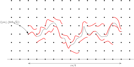
Figure 3. A visual depiction of the event $A^{(K),+}_{x,h,\delta,\varepsilon,n}$. The black curve in the middle depicts $\Lambda_{x,h}^{n}(\cdot)$. The short red curves depict pieces of the curves $\Lambda_{k\delta,\ell_{k}\sqrt{\delta}}^{n}(\cdot)$ and $\Lambda_{k\delta,(\ell_{k}+1)\sqrt{\delta}}^{n}(\cdot)$ which on the event $A^{(K),+}_{x,h,\delta,\varepsilon,n}$ do not meet.

To prove (31), the key observation is that if $\tau^{n}_{x,h}<\tau^{n}_{x^{\prime},h^{\prime}}$ then if the walk visits some site $\lfloor yn\rfloor$ between these two stopping times we must have that $\Lambda_{x,h}^{n}(y)<\Lambda_{x^{\prime},h^{\prime}}^{n}(y)$. Suppose now that $k\in\mathbb{Z}$ is such that $\lfloor xn\rfloor\leq\lfloor k\delta n\rfloor<\lfloor(k+1)\delta n\rfloor\leq\lfloor xn\rfloor+\frac{\varepsilon n}{4}$, and let $\ell_{k}\in\mathbb{Z}_{+}$ be such that $\frac{\lfloor 2\sigma\ell_{k}\sqrt{\delta n}\rfloor}{2\sigma\sqrt{n}}\leq\Lambda_{x,h}^{n}(k\delta)<\frac{\lfloor 2\sigma(\ell_{k}+1)\sqrt{\delta n}\rfloor}{2\sigma\sqrt{n}}$ (note that the integers $\ell_{k}$ defined in this way are random variables). Then the event $A^{(K)}_{x,h,\delta,\varepsilon,n}$ implies that

$$\Lambda_{k\delta,\ell_{k}\sqrt{\delta}}^{n}(y)\leq\Lambda_{x,h}^{n}(y)<\Lambda_{k\delta,(\ell_{k}+1)\sqrt{\delta}}^{n}(y),\qquad\forall y\in[k\delta,(k+1)\delta].$$

(See Figure 3 for a visual depiction of this.) To this end, for any $k\geq x/\delta$ if we define

$$S^{(K),k}_{x,h,\delta,n}=\left\{\ell_{k}\leq\frac{K}{\sqrt{\delta}}\text{ and }\Lambda_{k\delta,\ell_{k}\sqrt{\delta}}^{n}((k+1)\delta)<\Lambda_{k\delta,(\ell_{k}+1)\sqrt{\delta}}^{n}((k+1)\delta)\right\},$$

then we have that for $n$ sufficiently large

$$P\left(A^{(K),+}_{x,h,\delta,\varepsilon,n}\right)\leq P\left(\bigcap_{k=\frac{x}{\delta}}^{\frac{x}{\delta}+\lfloor\frac{\varepsilon}{5\delta}\rfloor}S^{(K),k}_{x,h,\delta,n}\right).$$

Note that if we fix some $k_{0}>x/\delta$ then the event $\bigcap_{k=\frac{x}{\delta}}^{k_{0}-1}S^{(K),k}_{x,h,\delta,n}$ gives information on the curves of various $\Lambda_{x^{\prime},h^{\prime}}^{n}(y)$ for $y\leq k_{0}\delta$. On the other hand, the only part of the event $S^{(K),k_{0}}_{x,h,\delta,n}$ that involves this information is the condition that $\ell_{k_{0}}\leq\frac{K}{\sqrt{\delta}}$. Therefore, it follows from the Markov property that

$$P\left(S^{(K),k_{0}}_{x,h,\delta,n}\,\biggl{|}\,\bigcap_{k=\frac{x}{\delta}}^{k_{0}-1}S^{(K),k}_{x,h,\delta,n}\right)\leq\max_{\ell\leq\frac{K}{\sqrt{\delta}}}P\left(\Lambda_{k_{0}\delta,\ell\sqrt{\delta}}^{n}((k_{0}+1)\delta)<\Lambda_{k_{0}\delta,(\ell+1)\sqrt{\delta}}^{n}((k_{0}+1)\delta)\right).$$

Repeatedly applying this, we then get that

$$P\left(A^{(K),+}_{x,h,\delta,\varepsilon,n}\right) \leq\prod_{k=\frac{x}{\delta}}^{\frac{x}{\delta}+\lfloor\frac{\varepsilon}{5\delta}\rfloor}\left\{\max_{\ell\leq\frac{K}{\sqrt{\delta}}}P\left(\Lambda_{k\delta,\ell\sqrt{\delta}}^{n}((k+1)\delta)<\Lambda_{k\delta,(\ell+1)\sqrt{\delta}}^{n}((k+1)\delta)\right)\right\}$$

$$\leq\left\{\max_{\frac{x}{\delta}\leq k\leq\frac{x}{\delta}+\lfloor\frac{\varepsilon}{5\delta}\rfloor}\max_{\ell\leq\frac{2K}{\sqrt{\delta}}}P\left(\Lambda_{k\delta,\ell\sqrt{\delta}}^{n}((k+1)\delta)<\Lambda_{k\delta,(\ell+1)\sqrt{\delta}}^{n}((k+1)\delta)\right)\right\}^{\left\lfloor\frac{\varepsilon}{5\delta}\right\rfloor},$$

and thus it follows from Theorem 4 that

$$\limsup_{n\to\infty}P\left(A^{(K),+}_{x,h,\delta,\varepsilon,n}\right) \leq\left\{\max_{\frac{x}{\delta}\leq k\leq\frac{x}{\delta}+\lfloor\frac{\varepsilon}{5\delta}\rfloor}\max_{\ell\leq\frac{2K}{\sqrt{\delta}}}P\left(\Lambda_{k\delta,\ell\sqrt{\delta}}((k+1)\delta)<\Lambda_{k\delta,(\ell+1)\sqrt{\delta}}((k+1)\delta)\right)\right\}^{\left\lfloor\frac{\varepsilon}{5\delta}\right\rfloor}$$

$$\leq\left\{\sup_{(k,\ell)\in\mathbb{Z}\times\mathbb{Z}_{+}}P\left(\Lambda_{k\delta,\ell\sqrt{\delta}}((k+1)\delta)<\Lambda_{k\delta,(\ell+1)\sqrt{\delta}}((k+1)\delta)\right)\right\}^{\left\lfloor\frac{\varepsilon}{5\delta}\right\rfloor}$$

(32) $$=\left\{\sup_{(k,\ell)\in\mathbb{Z}\times\mathbb{Z}_{+}}P\left(\Lambda_{k,\ell}(k+1)<\Lambda_{k,\ell+1}(k+1)\right)\right\}^{\left\lfloor\frac{\varepsilon}{5\delta}\right\rfloor},$$

where the last equality is due to the scaling properties of Brownian motion. Note that in applying Theorem 4 in the first line we are using convergence of the merging points, not the convergence of the curves. By the properties of the construction of the reflected/absorbed Brownian motions we have that

$$P\left(\Lambda_{k,\ell}(k+1)<\Lambda_{k,\ell+1}(k+1)\right)=\begin{cases}P\left(\Lambda_{-1,\ell}(0)<\Lambda_{-1,\ell+1}(0)\right)&\text{if }k\leq-1\\ P\left(\Lambda_{0,\ell}(1)<\Lambda_{0,\ell+1}(1)\right)&\text{if }k\geq 0.\end{cases}$$

All the probabilities on the right are less than 1 and as $\ell\to\infty$ they converge to the probability that two independent Brownian motions started a distance 1 apart do not meet in 1 unit of time, which is equal to $1-2\overline{\Phi}(2^{-1/2})$, where $\overline{\Phi}(t)=\int_{t}^{\infty}\frac{1}{\sqrt{2\pi}}e^{-x^{2}/2}\,dx$. Thus, it follows that the supremum inside the braces in (32) is strictly less than 1. In particular, we may choose $c_{0}>0$ such that

$$\sup_{(k,\ell)\in\mathbb{Z}\times\mathbb{Z}_{+}}P\left(\Lambda_{k,\ell}(k+1)<\Lambda_{k,\ell+1}(k+1)\right)<1-c_{0}.$$

It then follows from (32) that (31) holds for $n$ sufficiently large. ∎

Proposition 18.

The sequence of $\mathcal{D}$-valued random variables $(\mathcal{H}_{n})_{n\geq 1}$ is tight (with respect to the Skorokhod $J_{1}$ topology on ${\cal D}$), and moreover any subsequential limit is concentrated on paths that are continuous.

Proof.

Recall (14) and the notation $H_{n}=L(n,X_{n})$. The idea of the proof is rather simple. Since Proposition 17 implies that the walk doesn’t move a large distance in a short time, in order for the local time process $(H_{n})_{n\in\mathbb{Z}_{+}}$ to change by much in a short time either (1) the local time profile has to have a large fluctuation in a short distance or (2) the local time at a fixed location should increase very rapidly in a short amount of time. We will use the joint GRKT, Theorem 4, to show that both of these are unlikely to occur.

It is enough to show that for any $\varepsilon,\eta>0$ there is a $\delta^{\prime}>0$ such that

(33) $$\limsup_{n\to\infty}P\Bigg{(}\max_{\begin{subarray}{c}k,\ell\leq n^{3/2}\\ |k-\ell|\leq\delta^{\prime}n^{3/2}\end{subarray}}|H_{k}-H_{\ell}|>\varepsilon\sqrt{n}\Bigg{)}<\eta.$$

We note that similarly to (29)

(34) $$\Bigg{\{}\max_{\begin{subarray}{c}k,\ell\leq n^{3/2}\\ |k-\ell|\leq\delta^{\prime}n^{3/2}\end{subarray}}|H_{k}-H_{\ell}|\geq\varepsilon\sqrt{n}\Bigg{\}}\cap R_{K,n}\cap\left\{\operatorname{gap}(\mathcal{T}_{\delta,n}^{(K)})>\delta^{\prime}\right\}\subset\bigcup_{\begin{subarray}{c}x\in\delta\mathbb{Z}\cap[-K,K]\\ h\in\sqrt{\delta}\mathbb{Z}\cap[0,K]\end{subarray}}G^{(K)}_{x,h,\delta,\varepsilon,n},$$

where

$$G^{(K)}_{x,h,\delta,\varepsilon,n} =\left\{\exists j>\tau_{x,h}^{n}:\,\left|H_{j}-H_{\tau_{x,h}^{n}}\right|>\frac{\varepsilon}{4}\sqrt{n}\text{ and }\mathcal{T}_{\delta,n}\cap\left(\frac{\tau_{x,h}^{n}}{n^{3/2}},\frac{j}{n^{3/2}}\right)=\varnothing\right\}$$

$$\makebox[142.26378pt]{\ }\cap\left\{\max_{i\in\mathbb{Z}}L(\tau^{n}_{x,h},i)\leq 2\sigma K\sqrt{n}\right\}.$$

To bound $P(G^{(K)}_{x,h,\delta,\varepsilon,n})$ we will fix an $M\geq 1$ (to be chosen later) and then use (30) to conclude that for $n$ sufficiently large we have

(35) $$P(G^{(K)}_{x,h,\delta,\varepsilon,n})\leq 2(1-c_{0})^{\lfloor\frac{4\varepsilon^{2}}{5\delta M}\rfloor}+P\left(G^{(K)}_{x,h,\delta,\varepsilon,n}\setminus A^{(K)}_{x,h,\delta,\frac{4\varepsilon^{2}}{M},n}\right).$$

To bound the last probability, note that on the event $G^{(K)}_{x,h,\delta,\varepsilon,n}\setminus A^{(K)}_{x,h,\delta,\frac{4\varepsilon^{2}}{M},n}$ not only does the local time at the present location change by at least $\frac{\varepsilon}{4}\sqrt{n}$ before the next stopping time of the form $\tau_{x^{\prime},h^{\prime}}^{n}$ with $(x^{\prime},h^{\prime})\in\delta\mathbb{Z}\times\sqrt{\delta}\mathbb{Z}_{+}$, but it does so without moving a distance of more than $\frac{\varepsilon^{2}}{M}n$. Now, since

$$\left|H_{j}-H_{\tau_{x,h}^{n}}\right| =\left|L(j,X_{j})-L\left(\tau_{x,h}^{n},\lfloor xn\rfloor\right)\right|$$

$$\leq\left|L\left(j,X_{j}\right)-L(\tau_{x,h}^{n},X_{j})\right|+\left|L(\tau_{x,h}^{n},X_{j})-L\left(\tau_{x,h}^{n},\lfloor xn\rfloor\right)\right|,$$

we see that if the event $G^{(K)}_{x,h,\delta,\varepsilon,n}\setminus A^{(K)}_{x,h,\delta,\frac{4\varepsilon^{2}}{M},n}$ occurs, then either

1. there is an integer $k$ with $|k-\lfloor xn\rfloor|\leq n(\varepsilon^{2}/M)$ such that $|L(\tau_{x,h}^{n},k)-L(\tau_{x,h}^{n},\lfloor xn\rfloor)|\geq\frac{\varepsilon}{8}\sqrt{n}$, or equivalently, $\sup\limits_{y:|y-x|\leq\varepsilon^{2}/M}|\Lambda_{x,h}^{n}(y)-\Lambda_{x,h}^{n}(x)|\geq\frac{\varepsilon}{16\sigma}$,

2. or there is a time $j>\tau_{x,h}^{n}$ such that $|L(j,X_{j})-L(\tau_{x,h}^{n},X_{j})|\geq\frac{\varepsilon}{8}\sqrt{n}$ and such that there are no stopping times $\tau_{x^{\prime},h^{\prime}}^{n}\in(\tau_{x,h}^{n},j)$ with $(x^{\prime},h^{\prime})\in\delta\mathbb{Z}\times\sqrt{\delta}\mathbb{Z}_{+}$.

In the second case, let $k\in\mathbb{Z}$ be such that if $X_{j}\geq 0$ then $\lfloor k\delta n\rfloor\leq X_{j}<\lfloor(k+1)\delta n\rfloor$ or if $X_{j}<0$ then $\lfloor(k-1)\delta n\rfloor<X_{j}\leq\lfloor k\delta n\rfloor$, and then let $\ell\in\mathbb{Z}_{+}$ be such that $\tau_{k\delta,\ell\sqrt{\delta}}^{n}\leq\tau_{x,h}^{n}<j<\tau_{k\delta,(\ell+1)\sqrt{\delta}}^{n}$. Moreover, note that the conditions in the event $G^{(K)}_{x,h,\delta,\varepsilon,n}\setminus A^{(K)}_{x,h,\delta,\frac{4\varepsilon^{2}}{M},n}$ ensure that $|k|\leq(K+\frac{\varepsilon^{2}}{M})/\delta\leq 2K/\delta$ and $\ell\leq K/\sqrt{\delta}$. Then, it follows that

$$L\left(\tau_{k\delta,(\ell+1)\sqrt{\delta}}^{n},X_{j}\right)-L\left(\tau_{k\delta,\ell\sqrt{\delta}}^{n},X_{j}\right)\geq L(j,X_{j})-L(\tau_{x,h}^{n},X_{j})\geq\frac{\varepsilon}{8}\sqrt{n}.$$

If $X_{j}\geq 0$ then this implies that $\sup_{y\in[k\delta,(k+1)\delta)}\Lambda_{k\delta,(\ell+1)\sqrt{\delta}}^{n}(y)-\Lambda_{k\delta,\ell\sqrt{\delta}}^{n}(y)\geq\frac{\varepsilon}{16\sigma}$ while if $X_{j}<0$ then it implies that $\sup_{y\in((k-1)\delta,k\delta]}\Lambda_{k\delta,(\ell+1)\sqrt{\delta}}^{n}(y)-\Lambda_{k\delta,\ell\sqrt{\delta}}^{n}(y)\geq\frac{\varepsilon}{16\sigma}$. Therefore, it follows from the above consideration together with Theorem 4 that

(36) $$\limsup_{n\to\infty}P\left(G^{(K)}_{x,h,\delta,\varepsilon,n}\setminus A^{(K)}_{x,h,\delta,\frac{4\varepsilon^{2}}{M},n}\right)\leq P\left(\sup_{y:|y-x|\leq\frac{\varepsilon^{2}}{M}}|\Lambda_{x,h}(y)-h|\geq\frac{\varepsilon}{16\sigma}\right)$$

(37) $$\quad+\frac{12K^{2}}{\delta^{3/2}}\max_{\begin{subarray}{c}0\leq k\delta\leq K+\frac{\varepsilon^{2}}{M}\\ 0\leq\ell\sqrt{\delta}\leq K\end{subarray}}P\left(\sup_{y\in[k\delta,(k+1)\delta)}\Lambda_{k\delta,(\ell+1)\sqrt{\delta}}(y)-\Lambda_{k\delta,\ell\sqrt{\delta}}(y)\geq\frac{\varepsilon}{16\sigma}\right).$$

Recalling that the curves $\Lambda_{x,h}(\cdot)$ are reflected/absorbed Brownian motions, it follows that the second probability in (36) can be bounded in terms of a Brownian motion $B(\cdot)$:

$$P\left(\sup_{y:|y-x|\leq\frac{\varepsilon^{2}}{M}}|\Lambda_{x,h}(y)-h|\geq\frac{\varepsilon}{16\sigma}\right)\leq 4P\left(\sup_{0\leq t\leq\frac{\varepsilon^{2}}{M}}B(t)\geq\frac{\varepsilon}{16\sigma}\right)=8\overline{\Phi}\left(\frac{\sqrt{M}}{16\sigma}\right).$$

Similarly, for the probabilities in (37), since $\Lambda_{k\delta,\ell\sqrt{\delta}}(\cdot)$ and $\Lambda_{k\delta,(\ell+1)\sqrt{\delta}}(\cdot)$ are independent coalescing, reflected/absorbed Brownian motions then it follows that (as long as $\sqrt{\delta}<\frac{\varepsilon}{16\sigma}$)

$$P\left(\sup_{y\in[k\delta,(k+1)\delta)}\Lambda_{k\delta,(\ell+1)\sqrt{\delta}}(y)-\Lambda_{k\delta,\ell\sqrt{\delta}}(y)\geq\frac{\varepsilon}{16\sigma}\right)\\ \leq P\left(\sup_{0\leq t<\delta}\left(\sqrt{\delta}+\sqrt{2}B(t)\right)\geq\frac{\varepsilon}{16\sigma}\right)=2\overline{\Phi}\left(\frac{1}{\sqrt{2}}\left(\frac{\varepsilon}{16\sigma\sqrt{\delta}}-1\right)\right).$$

Combining these estimates with (34), (35), (36) and (37) we get that

$$\limsup_{n\to\infty} P\left(\max_{\begin{subarray}{c}k,\ell\leq n^{3/2}\\ |k-\ell|\leq\delta^{\prime}n^{3/2}\end{subarray}}|H_{k}-H_{\ell}|>\varepsilon\sqrt{n}\right)\leq\limsup_{n\to\infty}\left(P(R_{K,n}^{c})+P\left(\operatorname{gap}(\mathcal{T}_{\delta,n}^{(K)})\leq\delta^{\prime}\right)\right)$$

(38) $$\qquad+\frac{6K^{2}}{\delta^{3/2}}\left\{2(1-c_{0})^{\lfloor\frac{4\varepsilon^{2}}{5\delta M}\rfloor}+8\overline{\Phi}\left(\frac{\sqrt{M}}{16\sigma}\right)+\frac{24K^{2}}{\delta^{3/2}}\overline{\Phi}\left(\frac{1}{\sqrt{2}}\left(\frac{\varepsilon}{16\sigma\sqrt{\delta}}-1\right)\right)\right\}.$$

Finally, we show how the parameters $K$, $M$, $\delta$, and $\delta^{\prime}$ can be carefully chosen to make the right side smaller than $\eta$.

1. First, choose $K=K(\eta)$ as in Lemma 14.

2. Next, choose $M\geq 1$ and $\delta>0$ (depending on $K,\varepsilon,$ and $\eta$) so that (38) is less than $\eta/3$. For instance, this can be done by letting $M=\delta^{-1/2}$ and letting $\delta>0$ be sufficiently small.

3. Finally, choose $\delta^{\prime}>0$ (depending on $K$ and $\delta$) as in Lemma 15.

∎

Appendix A Associated urn processes

In this section we describe generalized Polya urn processes that can be used to study the TSAW. In particular, we will recall how these urn processes are connected with the processes of directed edge local times that play an important role in the proof of the joint GRKT for the TSAW (see Section 4).

Consider a generalization of the Polya urn process where if there are $r$ red balls and $b$ blue balls, then instead of drawing the balls uniformly at random the next ball drawn is red (resp., blue) with probability $\frac{\lambda^{2r-1}}{\lambda^{2b}+\lambda^{2r-1}}=\frac{\lambda^{2(r-b)-1}}{1+\lambda^{2(r-b)-1}}$ (resp. $\frac{1}{1+\lambda^{2(r-b)-1}}$) and then that ball is replaced in the urn along with another ball of the same color. Let $\mathfrak{R}_{j}$ and $\mathfrak{B}_{j}$ be the number of red and blue balls, respectively, in the urn after $n$ draws, and let $\mathfrak{D}_{j}=\mathfrak{R}_{j}-\mathfrak{B}_{j}$ be the discrepancy between the number of red and blue balls. Since the probability of drawing a red/blue ball depends only on the discrepancy, it is easy to see that the discrepancy process $(\mathfrak{D}_{j})_{j\geq 0}$ is a Markov chain with transition probabilities

$$P(\mathfrak{D}_{1}=i+1\mid\mathfrak{D}_{0}=i)=1-P(\mathfrak{D}_{1}=i-1\mid\mathfrak{D}_{0}=i)=\frac{\lambda^{2i-1}}{1+\lambda^{2i-1}},\qquad\forall i\in\mathbb{Z}.$$

This generalized urn process is connected with the TSAW as follows. If we fix a site $k\in\mathbb{Z}\setminus\{0\}$, then the sequence of right/left steps from $k$ on subsequent visits to $k$ has the same distribution as the urn discrepancy process $(\mathfrak{D}_{j})_{j\geq 0}$ (where a draw of a red ball corresponds to a step to the right and a blue ball corresponds to a step to the left) if we use the initial condition $\mathfrak{D}_{0}=0$ for sites $k\geq 1$ and the initial condition $\mathfrak{D}_{0}=1$ for sites $k\leq-1$. Similarly, the sequence of right/left steps from the origin correspond to a slightly different urn process $(\widetilde{\mathfrak{R}}_{j},\widetilde{\mathfrak{B}}_{j}),j\geq 0$, where the discrepancy $\widetilde{\mathfrak{D}}_{j}=\widetilde{\mathfrak{R}}_{j}-\widetilde{\mathfrak{B}}_{j}$ has transition probabilities given by

$$P(\widetilde{\mathfrak{D}}_{1}=i+1\mid\widetilde{\mathfrak{D}}_{0}=i)=1-P(\widetilde{\mathfrak{D}}_{1}=i-1\mid\widetilde{\mathfrak{D}}_{0}=i)=\frac{\lambda^{2i}}{1+\lambda^{2i}},\qquad\forall i\in\mathbb{Z},$$

and initial condition $\widetilde{\mathfrak{D}}_{0}=0$. Moreover, since transition probabilities for the TSAW only depend on the number of left and right steps from the current location, it follows that one can generate all of the steps of the TSAW at each site by running independent copies of the appropriate urn discrepancy process at each site.

Note that the distribution of the sequence of red/blue draws for the urn process $(\mathfrak{R}_{j},\mathfrak{B}_{j}),j\geq 0$, depends only on the initial discrepancy $\mathfrak{D}_{0}$ and not on the particular values of $\mathfrak{R}_{0}$ and $\mathfrak{B}_{0}$. Thus, below we will often use the notation $P_{i}(\cdot)=P(\cdot\mid\mathfrak{D}_{0}=i)$ for probabilities involving the urn process $(\mathfrak{R}_{j},\mathfrak{B}_{j}),j\geq 0$, started with discrepancy $\mathfrak{D}_{0}=i$.

A.1. Connection with directed edge local times

In this subsection we will explain how the distribution of the Markov chain of directed edge local times $(\mathcal{E}_{\tau_{k,m}}^{+}(\ell))_{\ell\geq k}$ which appears in the proof of the joint GRKT is related to the urn processes described above.

Let

$$\beta_{i}=\inf\{j\geq 1:\,\mathfrak{B}_{j}-\mathfrak{B}_{0}=i\},\quad\widetilde{\beta}_{i}=\inf\{j\geq 1:\,\widetilde{\mathfrak{B}}_{j}-\widetilde{\mathfrak{B}}_{0}=i\}$$

be the number of draws for the urn process $(\mathfrak{R}_{j},\mathfrak{B}_{j}),j\geq 0$, (resp. $(\widetilde{\mathfrak{R}}_{j},\widetilde{\mathfrak{B}}_{j}),j\geq 0$) until the $i$-th blue ball is drawn.

Lemma 19.

For any $k\in\mathbb{Z}$ and $m\geq 0$, $\{\mathcal{E}^{+}_{\tau_{k,m}}(\ell)\}_{\ell\geq k}$ is a (non-homogeneous) Markov chain with initial distribution supported on $\{0,1,\ldots,m\}$ so that

(39) $$\forall j\in\{0,1,\ldots,m\}\qquad P(\mathcal{E}^{+}_{\tau_{k,m}}(k)=j)=\begin{cases}P_{1}\left(\mathfrak{D}_{m}=2j-m+1\right)&\text{if }k\leq-1,\\ P_{0}\left(\widetilde{\mathfrak{D}}_{m}=2j-m\right)&\text{if }k=0,\\ P_{0}\left(\mathfrak{D}_{m}=2j-m\right)&\text{if }k\geq 1,\end{cases}$$

and with transition probabilities given by

(40) $$P\left(\mathcal{E}_{\tau_{k,m}}^{+}(\ell)=i+x\mid\mathcal{E}_{\tau_{k,m}}^{+}(\ell-1)=i\right)=\begin{cases}P_{1}\left(\mathfrak{D}_{\beta_{i+1}}=x\right)&\text{if }\ell\leq-1,\\ P_{0}\left(\widetilde{\mathfrak{D}}_{\tilde{\beta}_{i+1}}=x-1\right)&\text{if }\ell=0,\\ P_{0}\left(\mathfrak{D}_{\beta_{i}}=x\right)&\text{if }\ell\geq 1.\end{cases}$$

Proof.

For the distribution of the initial condition in (39), note that at time $\tau_{k,m}$ the walk has taken $m$ previous steps away from site $k$. Thus, $\mathcal{E}^{+}_{\tau_{k,m}}(k)=j$ if and only if $j$ of these steps have been to the right and $m-j$ of these steps have been to the left. Translating this to the corresponding urn process this means that the change in discrepancy must be $\mathfrak{D}_{m}-\mathfrak{D}_{0}=2j-m$ (or $\widetilde{\mathfrak{D}}_{m}-\widetilde{\mathfrak{D}}_{0}=2j-m$ in the case $k=0$).

For the transition probabilities in (40), we will explain only the case when $\ell\leq-1$ as the other cases are similar. In this case since the walk starts at $X_{0}=0$ and ends at $X_{\tau_{k,m}}=k<\ell<0$ then the walk will have taken one more step from $\ell$ to $\ell-1$ than it took from $\ell-1$ to $\ell$ by time $\tau_{k,m}$, and so the information $\mathcal{E}_{\tau_{k,m}}^{+}(\ell-1)=i$ means that the distribution of $\mathcal{E}_{\tau_{k,m}}^{+}(\ell)$ is determined by the urn process $(\mathfrak{R}_{j},\mathfrak{B}_{j}),j\geq 0$, for $j\leq\beta_{i+1}$. More precisely, $\mathcal{E}_{\tau_{k,m}}^{+}(\ell)=i+x$ if and only if there are $i+x$ red balls drawn before the $(i+1)$-st blue ball drawn, or equivalently if $\mathfrak{D}_{\beta_{i+1}}-\mathfrak{D}_{0}=x-1$. Since at sites $\ell\leq-1$ the discrepancy urn process starts at $\mathfrak{D}_{0}=1$ then we have that $P\left(\mathcal{E}_{\tau_{k,m}}^{+}(\ell)=i+x\mid\mathcal{E}_{\tau_{k,m}}^{+}(\ell-1)=i\right)=P_{1}\left(\mathfrak{D}_{\beta_{i+1}}=x\right)$. ∎

For the proof of the joint GRKT we will also need to know the joint distribution of multiple of these Markov chains corresponding to stopping times $\tau_{k_{1},m_{1}},\tau_{k_{2},m_{2}},\ldots,\tau_{k_{N},m_{N}}$. We omit the proof of the lemma below since it is essentially the same as the proof of Lemma 19.

Lemma 20.

For any $N\geq 1$ and any $k_{1},k_{2},\ldots,k_{N}\in\mathbb{Z}$ and $m_{1},m_{2},\ldots,m_{N}\geq 0$, the joint process $\left(\mathcal{E}^{+}_{\tau_{k_{1},m_{1}}}(\ell),\mathcal{E}^{+}_{\tau_{k_{2},m_{2}}}(\ell),\ldots,\mathcal{E}^{+}_{\tau_{k_{N},m_{N}}}(\ell)\right),\ell\geq\max\{k_{1},\ldots,k_{N}\}$, is a (non-homogeneous) Markov chain with transition probabilities given by

$$P\left(\mathcal{E}^{+}_{\tau_{k_{r},m_{r}}}(\ell)=i_{r}+x_{r},\,r=1,2,\ldots N\mid\mathcal{E}^{+}_{\tau_{k_{r},m_{r}}}(\ell-1)=i_{r},\,r=1,2,\ldots N\right)$$

$$\qquad=\begin{cases}P_{1}\left(\mathfrak{D}_{\beta_{i_{r}+1}}=x_{r},\,r=1,2,\ldots N\right)&\text{if }\ell\leq-1,\\ P_{0}\left(\widetilde{\mathfrak{D}}_{\tilde{\beta}_{i_{r}+1}}=x_{r}-1,\,r=1,2,\ldots N\right)&\text{if }\ell=0,\\ P_{0}\left(\mathfrak{D}_{\beta_{i_{r}}}=x_{r},\,r=1,2,\ldots N\right)&\text{if }\ell\geq 1.\end{cases}$$

A.2. Stationary distribution and convergence

The previous subsection showed the connection of the directed edge local times of the TSAW with the discrepancies in urn processes. Since the joint GRKTs involve scaling limits of the directed edge local times, it will be important to understand the distribution of $\mathfrak{D}_{j}$ and $\mathfrak{D}_{\beta_{j}}$ for $j$ large. The asymptotics of distributions of $\widetilde{\mathfrak{D}}_{j}$ and $\widetilde{\mathfrak{D}}_{\tilde{\beta}_{j}}$ are less important since they are only used for a single step of the directed edge local time process, but we will record these as well.

Since $(\mathfrak{D}_{j})_{j\geq 0}$ is a birth-death Markov chain, it is easy to use the detailed balance equations to show that it has stationary distribution $\rho(x)=C^{\prime}\lambda^{x(x-2)}\left(1+\lambda^{2x-1}\right)$, $x\in\mathbb{Z}$, where $C^{\prime}>0$ is an appropriate normalizing constant. Similarly, the stationary distribution for $(\widetilde{\mathfrak{D}}_{j})_{j\geq 0}$ is $\tilde{\rho}(x)=\widetilde{C}^{\prime}\lambda^{x(x-1)}(1+\lambda^{2x})$, $x\in\mathbb{Z}$.

Since the discrepancy process $(\mathfrak{D}_{j})_{j\geq 0}$ is positive recurrent, the urn will asymptotically have roughly the same number of red and blue balls. In fact, it is not hard to show from this that $\lim_{j\to\infty}\frac{\beta_{j}}{j}=2$, and from this we can use the ergodic theorem for Markov chains to identify the stationary distribution for $(\mathfrak{D}_{\beta_{j}})_{j\geq 0}$ as

$$\pi(x)=\lim_{j\to\infty}\frac{1}{j}\sum_{i=1}^{j}\mathbbm{1}_{\{\mathfrak{D}_{\beta_{i}}=x\}} =\lim_{j\to\infty}\left(\frac{\beta_{j}}{j}\right)\left(\frac{1}{\beta_{j}}\sum_{m=1}^{\beta_{j}}\mathbbm{1}_{\{\mathfrak{D}_{m-1}=x+1,\,\mathfrak{D}_{m}=x\}}\right)$$

$$=2\rho(x+1)\frac{1}{1+\lambda^{2x+1}}=2C^{\prime}\lambda^{x^{2}-1}=:C\lambda^{x^{2}},\qquad\forall x\in\mathbb{Z}.$$

Similarly, the stationary distribution for $(\widetilde{\mathfrak{D}}_{\tilde{\beta}_{j}})_{j\geq 0}$ is $\tilde{\pi}(x)=2\widetilde{C}^{\prime}\lambda^{(x+1)x}$. Moreover, the convergence of the distribution of $\mathfrak{D}_{\beta_{j}}$ to $\pi$ is exponentially fast. In fact, the following proposition gives exponential bounds on the total variation distance of the distribution of $(\mathfrak{D}_{\beta_{j_{1}}},\mathfrak{D}_{\beta_{j_{2}}},\ldots,\mathfrak{D}_{\beta_{j_{N}}})$ from $\pi^{\otimes N}$. We have already stated this fact in Proposition 10 using the equivalent notation (see Lemma 20) of directed edge local times. A similar result can also be proven for the Markov chain $(\widetilde{\mathfrak{D}}_{\tilde{\beta}_{j}})_{j\geq 0}$, but we will not need such a result in the present paper.

Proposition 10 (restated).

There are constants $C_{2}$ and $C_{3}$ such that for any $N\in\mathbb{N}$ and any choice of $0=n_{0}<n_{1}<n_{2}<n_{3}<\cdots<n_{N}$ we have for $x\in\{0,1\}$ that

(41) $$\sum_{k_{1},k_{2},\ldots,k_{N}\in\mathbb{Z}}\left|P_{x}\left(\mathfrak{D}_{\beta_{n_{i}}}=k_{i},\,i=1,2,\ldots,N\right)-\prod_{i=1}^{N}\pi(k_{i})\right|\leq C_{3}\sum_{i=1}^{N}e^{-C_{2}(n_{i}-n_{i-1})}.$$

Proof.

The one dimensional case $N=1$ was proved in [Tót95, Lemma 1]. In fact, in the proof of that Lemma it was shown that the renewal times of the Markov $\mathfrak{D}_{\beta_{n}}$ have exponential moments (see (3.13) in [Tót95]). Thus, it follows from [Num84, Theorem 6.14 and Example 5.5(a)] that for every $j\in\mathbb{Z}$ there is a constant $M(j)<\infty$ such that

(42) $$\sum_{k\in\mathbb{Z}}\left|P_{j}\left(\mathfrak{D}_{\beta_{n}}=k\right)-\pi(k)\right|\leq M(j)e^{-C_{2}n},\qquad\forall n\geq 1,$$

and, moreover, that the constants $M(j)$ are such that

(43) $$\overline{M}:=\sum_{k\in\mathbb{Z}}\pi(k)M(k)<\infty.$$

The proof of (41) with $C_{3}=\max\{M(0),M(1),\overline{M}\}$ then follows rather easily from (42) and (43) using induction on $N\geq 1$. ∎

Remark 21.

We close this section by noting that the stationary distributions $\pi$ and $\tilde{\pi}$ can be used to give tail estimates on $\mathfrak{D}_{\beta_{n}}$ and $\widetilde{\mathfrak{D}}_{\tilde{\beta}_{n}}$ that are uniform in $n$. Indeed, we have $P_{i}(\mathfrak{D}_{\beta_{n}}=j)\leq\frac{\pi(j)}{\pi(i)}$ and $P_{i}(\widetilde{\mathfrak{D}}_{\tilde{\beta}_{n}}=j)\leq\frac{\tilde{\pi}(j)}{\tilde{\pi}(i)}$, for all $i,j\in\mathbb{Z}$ and $n\geq 1$. Together with Lemma 19 this implies that the increments of the directed edge local time processes $(\mathcal{E}_{k,m}^{+}(\ell))_{\ell\geq k}$ have uniform Gaussian tails. This fact will be used in Appendix C below.

Appendix B Relating the backward and the forward paths

The following is the analog of equation (21) for the TSRM. Note that this formula differs from the definition of the backward paths in [TW98, p. 389] because this paper uses a slightly different version of stopping times.

Lemma 22.

For $y\neq x$ and $h\geq 0$, $\Lambda_{x,h}(y)=\inf\left\{h^{\prime}\geq 0:\Lambda_{y,h^{\prime}}(x)>h\right\}$, almost surely.

Proof.

It follows from the definition of $\mathfrak{t}_{x,h}$ and the relation $h=\Lambda_{x,h}(x)=\mathfrak{L}(\mathfrak{t}_{x,h},x)$ that

(44) $$s>\mathfrak{t}_{x,h}\iff\mathfrak{L}(s,x)>h.$$

Next, note that

$$\Lambda_{x,h}(y)=0 \iff\mathfrak{L}(\mathfrak{t}_{x,h},y)=0=\mathfrak{L}(\mathfrak{t}_{y,0},y)$$

$$\iff\mathfrak{t}_{x,h}<\mathfrak{t}_{y,0}\qquad\text{(Recall that $\mathfrak{t}_{x,h}\neq\mathfrak{t}_{y,0}$, almost surely)}$$

$$\iff\mathfrak{t}_{x,h}<\mathfrak{t}_{y,h^{\prime}}\quad\forall h^{\prime}>0\qquad\text{(using $\mathfrak{t}_{y,0}=\lim_{h^{\prime}\to 0^{+}}\mathfrak{t}_{y,h^{\prime}}$ and $\mathfrak{t}_{x,h}\neq\mathfrak{t}_{y,0}$ almost surely)}$$

$$\overset{\eqref{txhprop}}{\iff}\Lambda_{y,h^{\prime}}(x)=\mathfrak{L}(\mathfrak{t}_{y,h^{\prime}},x)>h,\quad\forall h^{\prime}>0$$

$$\iff\inf\left\{h^{\prime}\geq 0:\Lambda_{y,h^{\prime}}(x)>h\right\}=0.$$

Similarly, if $\Lambda_{x,h}(y)=\mathfrak{L}(\mathfrak{t}_{x,h},y)=b$ then the definition of $\mathfrak{t}_{y,b}$ implies that $\mathfrak{t}_{x,h}\leq\mathfrak{t}_{y,b}$, but since these times are almost surely not equal then we have $\mathfrak{t}_{x,h}<\mathfrak{t}_{y,b}$. Moreover, for any $h^{\prime}\in[0,b)$ we have that $b>h^{\prime}=\mathfrak{L}(\mathfrak{t}_{y,h^{\prime}},y)$ so that $\mathfrak{t}_{y,h^{\prime}}<\mathfrak{t}_{x,h}$ for all $h^{\prime}\in[0,b)$. Conversely, suppose that $\mathfrak{t}_{y,h^{\prime}}<\mathfrak{t}_{x,h}<\mathfrak{t}_{y,b}$ for all $h^{\prime}\in[0,b)$. The second inequality implies that $\Lambda_{x,h}(y)=\mathfrak{L}(\mathfrak{t}_{x,h},y)\leq\mathfrak{L}(\mathfrak{t}_{y,b},y)=b$, while the first inequality implies (by (44)) that $\Lambda_{x,h}(y)=\mathfrak{L}(\mathfrak{t}_{x,h},y)>h^{\prime}$. Since this holds for all $h^{\prime}\in[0,b)$ these together imply that $\Lambda_{x,h}(y)=b$. Using the above argument to get the first $\iff$ in the display below, we see that

$$\Lambda_{x,h}(y)=b \iff\mathfrak{t}_{y,h^{\prime}}<\mathfrak{t}_{x,h}<\mathfrak{t}_{y,b},\quad\forall h^{\prime}\in[0,b)$$

$$\iff\mathfrak{t}_{y,h^{\prime}}<\mathfrak{t}_{x,h}<\mathfrak{t}_{y,h^{\prime\prime}},\quad\forall h^{\prime}\in[0,b)\text{ and }\forall h^{\prime\prime}>b$$

$$\overset{\eqref{txhprop}}{\iff}\Lambda_{y,h^{\prime}}(x)\leq h<\Lambda_{y,h^{\prime\prime}}(x),\quad\forall h^{\prime}\in[0,b)\text{ and }\forall h^{\prime\prime}>b$$

$$\iff\inf\left\{h^{\prime}\geq 0:\Lambda_{y,h^{\prime}}(x)>h\right\}=b.$$

Note that the second line holds since $h^{\prime\prime}\mapsto\mathfrak{t}_{y,h^{\prime\prime}}$ is right continuous by the definition in (7) and the fact that $t\mapsto\mathfrak{L}(t,y)$ is almost surely continuous as shown in [TW98]. This completes the proof of the lemma. ∎

We record the following useful corollary.

Corollary 23.

For any $x\neq y$ and $h,h^{\prime}\geq 0$, with probability 1 we have

(45) $$\left\{\Lambda_{y,h^{\prime}}(x)<h\right\}\subset\left\{\Lambda_{x,h}(y)>h^{\prime}\right\}\subset\left\{\Lambda_{y,h^{\prime}}(x)\leq h\right\}\subset\left\{\Lambda_{x,h}(y)\geq h^{\prime}\right\}.$$

Proof.

First of all, since $\Lambda_{y,h^{\prime}}(x)=\lim_{\varepsilon\to 0^{+}}\Lambda_{y,h^{\prime}+\varepsilon}(x)$, almost surely (see Remark 2 on p. 387 and Theorem 4.3 in [TW98]), it follows that

$$\Lambda_{y,h^{\prime}}(x)<h\ \Longrightarrow\ h^{\prime}\notin\overline{\{b\geq 0:\Lambda_{y,b}(x)>h\}}\ \overset{\text{Lem.\,}\ref{lem:TSRMweave}}{\iff}\ h^{\prime}<\Lambda_{x,h}(y)$$

This proves the first inclusion in (45). The second inclusion follows easily from Lemma 22 because $\Lambda_{x,h}(y)>h^{\prime}$ implies that $h^{\prime}\notin\{b\geq 0:\Lambda_{y,b}(x)>h\}$. Finally, the third inclusion in (45) follows from the first inclusion by taking complements of both sets and reversing the roles of $(x,h)$ and $(y,h^{\prime})$. ∎

Appendix C Gambler’s ruin estimates

The main statement in this section is Lemma 27. It gives gambler’s ruin sort of estimates for the difference of two discrete local time curves. These estimates are not optimal but they are sufficient to give us Corollary 28 which is a crucial technical result needed for the proof of convergence of the merge points of a pair of local time curves in the joint forward GRKT, Theorem 12.

C.1. Preliminaries

Recall the notation for $S^{n}_{i}$ introduced in (19). Parameters $n$ and $x<0$ will be fixed throughout this section, so we shall drop them from the notation. The cases $x=0$ and $x>0$ will not be considered separately as their treatment requires only minor changes.

We shall first consider a single process $S(j),\ j\in\mathbb{Z}_{+}$, associated to the directed edge local times as defined in (19) without specifying the initial state (and dropping all indices). Let $\xi(j):=S(j)-S(j-1)$ be its increments, $\zeta(j),j\in\mathbb{N}$, be i.i.d. $\pi$-distributed random variables, and $Y(j)=Y(0)+\sum_{i=1}^{j}\zeta(j)$, $j\in\mathbb{N}$.

The lemma below is an easy consequence of Proposition 10 with $N=1$ (which was already contained in [Tót95]). Set $S_{*}(j)=\min_{i\leq j}S(i)$ and $Y_{*}(j)=\min_{i\leq j}Y(i)$.

Lemma 24 (Coupling lemma).

Let $b\geq 2$, $S(0)=Y(0)=b$, and the walks $S$ and $Y$ be coupled using the maximal coupling of their increments. Denote the decoupling time by $\gamma:=\min\{j\in\mathbb{N}:\xi(j)\neq\zeta(j)\}$. Then for any $\delta>0$

(46) $$P(\gamma>b^{2-\delta})\to 1\ \ \text{as }b\to\infty.$$

(47) $$P(S_{*}(\lfloor b^{2-\delta}\rfloor)>b/2)\to 1\ \ \text{as }b\to\infty.$$

Proof.

Note that (47) follows from (46) and the invariance principle for random walks.

$$P(\gamma>b^{2-\delta}) \geq P\left(\gamma>b^{2-\delta},S_{*}(\lfloor b^{2-\delta}\rfloor)>b/2\right)=P\left(\gamma>b^{2-\delta},Y_{*}(\lfloor b^{2-\delta}\rfloor)>b/2\right)$$

$$=P\left(\gamma>b^{2-\delta}\mid Y_{*}(\lfloor b^{2-\delta}\rfloor)>b/2\right)P\left(Y_{*}(\lfloor b^{2-\delta}\rfloor)>b/2\right)$$

$$\geq\left(1-C_{3}e^{-C_{2}b/2}\right)^{\lfloor b^{2-\delta}\rfloor}P\left(Y_{*}(\lfloor b^{2-\delta}\rfloor)-Y(0)>-b/2\right)\to 1\ \ \text{as}\ b\to\infty.$$

In the last line we used the invariance principle for a mean 0 random walk. ∎

Suppose now that we have two coalescing reflected/absorbed random walks $S_{1}\leq S_{2}$ as above constructed from directed edge local times to the right from $x<0$ of the same TSAW. We want to show that if $S_{1}(0)\geq b^{4}$ and $0\leq S_{2}(0)-S_{1}(0)<b$ then with probability tending to 1 as $b\to\infty$ they will coalesce by time $b^{7}$ and before $S_{1}$ goes below $b^{4}/2$.

We know from Lemma 24 with $b$ replaced by $b^{4}$ and $\delta=1/4$ that $P(S_{1*}(b^{7})>b^{4}/2)\to 1$ as $b\to\infty$ and that the probability that the coupling of $S_{1}$ with $Y_{1}$ ($Y_{1}$ is the walk with independent $\pi$-distributed increments coupled to $S_{1}$ ) does not break down up to time $b^{7}$ also goes to 1. Hence, on the intersection of these two events we can replace $S_{1}$ with $Y_{1}$. We can do the same for $S_{2}$ but, as $S_{1}$ and $S_{2}$ get close, the walks $Y_{1}$ and $Y_{2}$ will be non-negligibly correlated.

Note that if $Y_{1}$ and $Y_{2}$ were independent, then their difference would be a mean 0 random walk with independent increments distributed according to $\pi_{2}(\cdot):=\sum_{y\in\mathbb{Z}}\pi(y)\pi(y+\cdot)$. Note that $\pi_{2}$ is symmetric with a superexponential tail decay, so the hitting time of $0$ by $Y_{2}-Y_{1}$ would obey standard estimates (see, for instance, [LL10, Section 5.1.1]). In our case, $S_{\Delta}(j):=S_{2}(j)-S_{1}(j),\ j\geq 0$, is not Markov, and we shall need both coordinates to have a Markov process. Let $\Delta(j):=S_{2}(j)-S_{2}(j-1)-(S_{1}(j)-S_{1}(j-1))$, $j\geq 1$, be the increments of the difference of the two walks.

To satisfy the non-trapping conditions in [Tót95] (see (4.10), (4.11)), we shall modify our processes as follows. If the walks coalesce before $S_{1}$ gets absorbed then from the time they coalesce we let them follow two independent random walks with the step distribution $\pi$; if $S_{1}$ gets absorbed before they coalesce then we re-start it from 1. These modifications will not matter for our applications. The modified processes will be denoted by $(\widetilde{S}_{1},\widetilde{S}_{2})$. We also set

$$P_{n_{1},m}(\cdot):=P(\cdot\mid\widetilde{S}_{1}(0)=n_{1},\widetilde{S}_{2}(0)=n_{1}+m)$$

and similarly for the expectation.

Define

$$p_{\Delta}(k|n_{1},m): =P_{n_{1},m}(\Delta(1)=k)$$

$$=\sum_{y\in\mathbb{Z}}P_{n_{1},m}(\widetilde{S}_{1}(j)=n_{1}+y,\widetilde{S}_{2}(j)=n_{1}+m+y+k)$$

Recall that $\pi_{2}(k)=P(\zeta(2)-\zeta(1)=k)$. Note that $\pi_{2}(k)=\pi_{2}(-k)$ and its tails are bounded by $C\lambda^{k^{2}/2}$. From Proposition 10 we get

(48) $$\sum_{k\in\mathbb{Z}}|p_{\Delta}(k|n_{1},m)-\pi_{2}(k)|\leq 2C_{3}e^{-C_{2}(n_{1}\wedge m)},$$

Since $|E_{n_{1},m}[\Delta(1)]|\leq|E_{n_{1},m}[\widetilde{S}_{2}(1)-(n_{1}+m)]|+|E_{n_{1},m}[\widetilde{S}_{1}(1)-n_{1}]|$, Proposition 10 (for $N=1$), the symmetry of $\pi$, and the exponential decay of the tails of $\xi$ (see Remark 21) imply that

(49) $$\Big{|}\sum_{k\in\mathbb{Z}}kp_{\Delta}(k|n_{1},m)\Big{|} =|E_{n_{1},m}[\Delta(1)]|\leq C_{4}e^{-C_{5}n_{1}}\ \ \text{with }C_{5}=C_{2}/2,$$

and

$$\liminf_{n_{1}\wedge m\to\infty}\sum_{k\in\mathbb{Z}}p_{\Delta}(k|n_{1},m)e^{-C_{5}k} \geq\sum_{k\in\mathbb{Z}}\pi_{2}(k)e^{-C_{5}k}$$

(50) $$=\pi_{2}(0) +\sum_{k\in\mathbb{N}}\pi_{2}(k)\left(e^{-C_{5}k}+e^{C_{5}k}\right)>\pi_{2}(0)+\sum_{k\neq 0}\pi_{2}(k)=1.$$

Now we can choose $a_{1}\in\mathbb{N}$ and a constant $C_{6}$ so that for $n_{1}\wedge m\geq a_{1}$,

(51) $$C_{6}\left(\sum_{k\in\mathbb{Z}}p_{\Delta}(k|n_{1},m)e^{-C_{5}k}-1\right)\geq C_{4}.$$

Lemma 25.

Let $a_{1}\in\mathbb{N}$ be chosen so that (51) holds. Then for $n_{1}\geq m\geq a_{1}$

$$E_{n_{1},m}\left[\pm\widetilde{S}_{\Delta}(1)+C_{6}e^{-C_{5}\widetilde{S}_{\Delta}(1)}\right]\geq\pm m+C_{6}e^{-C_{5}m}.$$

Hence, as long as $\widetilde{S}_{1}(j)\geq\widetilde{S}_{\Delta}(j)\geq a_{1}$, the processes $\pm\widetilde{S}_{\Delta}(j)+C_{6}e^{-C_{5}\widetilde{S}_{\Delta}(j)},\ j\geq 0$, are submartingales relative to the natural filtration of $(\widetilde{S}_{1},\widetilde{S}_{\Delta})$.

Proof.

By (49) and (51),

$$E_{n_{1},m}\left[\pm\Delta(1)+C_{6}e^{-C_{5}m}(e^{-C_{5}\Delta(1)}-1)\right]\geq\\ -C_{4}e^{-C_{5}(n_{1}\wedge m)}+C_{6}e^{-C_{5}m}\left(\sum_{k\in\mathbb{Z}}p_{\Delta}(k|n_{1},n_{1}+m)e^{-C_{5}k}-1\right)\geq 0.$$

∎

C.2. Gambler’s ruin for a modified process.

Fix an arbitrary integer $b\geq 2$. All quantities related to modified processes introduced below depend on $b$. But we shall not reflect this fact in our notation. Let $\alpha:=\inf\{j\geq 0:\widetilde{S}_{1}(j)<b\}$. To adapt the proof of [Tót95, Lemma 3] to our setting we shall first prove the result for the process $\widetilde{S}_{\Delta}$ modified starting at time $\alpha$. Namely,

$$\check{S}_{\Delta}(\ell+1)-\check{S}_{\Delta}(\ell) :=\begin{cases}\widetilde{S}_{2}(\ell+1)-\widetilde{S}_{2}(\ell)-(\widetilde{S}_{1}(\ell+1)-\widetilde{S}_{1}(\ell)),&\text{if }\ell<\alpha;\\ \chi(\ell+1),&\text{if }\ell\geq\alpha,\end{cases}$$

where $\chi(\ell),\ell\in\mathbb{N}_{0}$, are i.i.d. uniform on $\{-1,1\}$ random variables independent of everything else. In words, once $\widetilde{S}_{1}$ falls below $b$, the process $\check{S}_{\Delta}$ “forgets” about $\widetilde{S}_{1}$ and starts following an independent simple symmetric random walk.

For an interval ${\cal I}\subset[0,\infty)$ define $\check{\theta}_{\cal I}=\inf\{\ell\geq 0:\check{S}_{\Delta}(\ell)\not\in{\cal I}\}$. The bounds stated in the next lemma are the analogs of (A4.5) and (A4.6) in [Tót95].

Lemma 26 (Overshoot lemma).

There is a constant $C_{7}>0$ such that for all $b\geq 2$, $a\in[0,b-2]\cap\mathbb{Z}$, $n_{1}\in\mathbb{Z}_{+}$, and $m\in(a,b)\cap\mathbb{Z}$

(52) $$E_{n_{1},m}(\check{S}_{\Delta}(\check{\theta}_{(a,b)})|\check{S}_{\Delta}(\check{\theta}_{(a,b)})\geq b) \leq b+C_{7};$$

(53) $$E_{n_{1},m}(\check{S}^{2}_{\Delta}(\check{\theta}_{(a,b)})|\check{S}_{\Delta}(\check{\theta}_{(a,b)})\geq b) \leq(b+C_{7})^{2}.$$

The bound (52) follows from (53). We will prove (53) in Appendix D.

Given (48)-(53), the proof of the next lemma is very similar to the one of [Tót95, Lemma 3].

Lemma 27.

1. There exists a constant $C_{8}>0$ such that for all $b\geq 2$, $n_{1}\in\mathbb{Z}_{+}$, and $m\in(0,b)\cap\mathbb{Z}$

   $$P_{n_{1},m}(\check{S}_{\Delta}(\check{\theta}_{(0,b)})=0)>\frac{b-m}{b+C_{8}}.$$

2. There exists a constant $C_{9}>0$ such that for all $b\geq 2$, $n_{1}\in\mathbb{Z}_{+}$, and $m\in[0,b)\cap\mathbb{Z}_{+}$

   $$E_{n_{1},m}[\check{\theta}_{[0,b)}]\leq C_{9}b^{3}.$$

Proof.

Note that if $n_{1}<b$ then $\check{S}_{\Delta}$ follows a simple symmetric random walk for which both statements hold by the standard Gambler’s ruin estimates. Thus, we shall assume that $n_{1}\geq b$. Without loss of generality we also suppose that $b>a_{1}+1+C_{7}$, where $a_{1}$ is defined just above (51) and $C_{7}$ is from (52).

(a) Let $a_{1}<m<b$ and $f(s)=-s+C_{6}e^{-C_{5}s}$. Note that the process $f(\check{S}_{\Delta}(j\wedge\check{\theta}_{(a_{1},b)})),\ j\geq 0$, is a submartingale relative to filtration ${\cal G}_{j}:=\sigma(\widetilde{S}_{1}(\ell),\check{S}_{\Delta}(\ell),\chi(\ell),\ 0\leq\ell\leq j)$, $j\geq 0$. Indeed, either $\widetilde{S}_{1}$ stays above $b$ and, thus, above $\check{S}_{\Delta}$ up to time $\check{\theta}_{(a_{1},b)}$, and the conditions of Lemma 25 are satisfied, or, if prior to $\check{\theta}_{(a_{1},b)}$ the process $\widetilde{S}_{1}$ goes below $b$, $\check{S}_{\Delta}$ switches to a simple symmetric random walk. By the optional stopping theorem and monotonicity of the function $f$,

$$b-m <f(m)-f(b)\leq E_{n_{1},m}(f(\check{S}_{\Delta}(\check{\theta}_{(a_{1},b)}))-f(b))$$

$$\leq E_{n_{1},m}(f(\check{S}_{\Delta}(\check{\theta}_{(a_{1},b)}))-f(b)\mid\check{S}_{\Delta}(\check{\theta}_{(a_{1},b)})\leq a_{1})P_{n_{1},m}(\check{S}_{\Delta}(\check{\theta}_{(a_{1},b)})\leq a_{1})$$

$$<\left(b+C_{6}-E_{n_{1},m}(\check{S}_{\Delta}(\check{\theta}_{(a_{1},b)})\mid\check{S}_{\Delta}(\check{\theta}_{(a_{1},b)})\leq a_{1})\right)P_{n_{1},m}(\check{S}_{\Delta}(\check{\theta}_{(a_{1},b)})\leq a_{1})$$

Since $\check{S}_{\Delta}(\check{\theta}_{(a_{1},b)})\geq 0$, we get that for $a_{1}<m<b$

(54) $$P_{n_{1},m}(\check{S}_{\Delta}(\check{\theta}_{(a_{1},b)})\leq a_{1})>\frac{b-m}{b+C_{6}}.$$

Note that, by the remark made at the start of the proof, the above inequality holds for all $(n_{1},m)\in\{(n_{1},m)\in\mathbb{Z}_{+}^{2}\mid n_{1}<b\ \text{or}\ (n_{1}\geq b\ \text{and}\ a_{1}<m<b)\}$

Let us consider the case $0<m\leq a_{1}$. Using (54) we get

$$P_{n_{1},m}(\check{S}_{\Delta}(\check{\theta}_{(0,b)})=0)\\ \geq P_{n_{1},m}(\check{S}_{\Delta}(\check{\theta}_{(0,a_{1}]})=0)+\sum_{m\geq 0}P_{n_{1},m}\left(\check{S}_{\Delta}(\check{\theta}_{(0,a_{1}]})>a_{1},\widetilde{S}_{1}(\check{\theta}_{(0,a_{1}]})=m\right)\\ \times\sum_{a_{1}<j<b}P_{n_{1},m}\left(\check{S}_{\Delta}(\check{\theta}_{(0,a_{1}]})=j\mid\check{S}_{\Delta}(\check{\theta}_{(0,a_{1}]})>a_{1},\widetilde{S}_{1}(\check{\theta}_{(0,a_{1}]})=m\right)\frac{b-j}{b+C_{6}}\\ \times\inf_{0<m^{\prime}\leq a_{1},n_{1}^{\prime}\in\mathbb{Z}_{+}}P_{n_{1}^{\prime},m^{\prime}}(\check{S}_{\Delta}(\check{\theta}_{(0,b)})=0)$$

Rearranging the right hand side and using (52) we see that

$$P_{n_{1},m}(\check{S}_{\Delta}(\check{\theta}_{(0,b)})=0)\geq P_{n_{1},m}(\check{S}_{\Delta}(\check{\theta}_{(0,a_{1}]})=0)\\ +\frac{b-a_{1}-1-C_{7}}{b+C_{6}}P_{n_{1},m}\left(\check{S}_{\Delta}(\check{\theta}_{(0,a_{1}]})>a_{1}\right)\inf_{0<m^{\prime}\leq a_{1},n_{1}^{\prime}\in\mathbb{Z}_{+}}P_{n_{1}^{\prime},m^{\prime}}(\check{S}_{\Delta}(\check{\theta}_{(0,b)})=0)\\ =\left(1-\frac{b-a_{1}-1-C_{7}}{b+C_{6}}\inf_{0<m^{\prime}\leq a_{1},n_{1}^{\prime}\in\mathbb{Z}_{+}}P_{n_{1}^{\prime},m^{\prime}}(\check{S}_{\Delta}(\check{\theta}_{(0,b)})=0)\right)P_{n_{1},m}(\check{S}_{\Delta}(\check{\theta}_{(0,a_{1}]})=0)\\ +\frac{b-a_{1}-1-C_{7}}{b+C_{6}}\inf_{0<m^{\prime}\leq a_{1},n_{1}^{\prime}\in\mathbb{Z}_{+}}P_{n_{1}^{\prime},m^{\prime}}(\check{S}_{\Delta}(\check{\theta}_{(0,b)})=0).$$

We note that for all $m\leq a_{1}$ and $n_{1}\in\mathbb{Z}_{+}$

$$P_{n_{1},m}(\check{S}_{\Delta}(\check{\theta}_{(0,a_{1}]})=0)\geq P_{n_{1},m}(\check{S}_{\Delta}(1)=0) \geq P_{n_{1},a_{1}}(\check{S}_{\Delta}(1)=0\mid\check{S}_{1}(1)\geq n_{1})P_{n_{1}}(\check{S_{1}}(1)\geq n_{1})$$

$$\geq\left(1+\lambda^{-2a_{1}-1}\right)^{-a_{1}}P_{n_{1}}(\check{S_{1}}(1)\geq n_{1}).$$

Since for all large $n_{1}$ the distribution of $\check{S}_{1}(1)-\check{S}_{1}(0)$ is close to $\pi$, we get that

$$\inf_{0<m^{\prime}\leq a_{1},n_{1}^{\prime}\in\mathbb{Z}_{+}}P_{n_{1}^{\prime},m^{\prime}}(\check{S}_{\Delta}(\check{\theta}_{(0,a_{1}]})=0)=:C_{10}>0,$$

and

(55) $$\inf_{0<m^{\prime}\leq a_{1},n_{1}^{\prime}\in\mathbb{Z}_{+}}P_{n_{1}^{\prime},m^{\prime}}(\check{S}_{\Delta}(\check{\theta}_{(0,b)})=0)\geq\frac{C_{10}(b+C_{6})}{C_{10}b+C_{6}+(1-C_{10})(a_{1}+1+C_{7})}.$$

Inequalities (54) and (55) imply part (a).

(b) We shall first show that there is a constant $C_{11}>0$ such that for all $n_{1}\in\mathbb{Z}_{+}$ and integers $a$ and $m$ satisfying $0\leq a<m<b$,

(56) $$P_{n_{1},m}(\check{S}_{\Delta}(\check{\theta}_{(a,b)})\geq b)>C_{11}\frac{m-a}{b-a}.$$

Let $a_{2}=a_{1}\vee C_{6}$, $g(s)=s+C_{6}e^{-C_{5}s}$, and assume that $a_{2}\leq a<b$ and $\check{S}_{\Delta}(0)=m\in(a,b)$. Consider the submartingale $g(\check{S}_{\Delta}(j\wedge\check{\theta}_{(a,b)})),\ j\geq 0$. Note that, by convexity of $g$ and the fact that $g(0)=C_{6}<a<g(a)$, if $0\leq\check{S}_{\Delta}(j)<a$ then $g(\check{S}_{\Delta}(j))<g(a)$. Using this observation and (52) we get

$$g(m)-g(a)\leq E_{n_{1},m}\left(g(\check{S}_{\Delta}(\check{\theta}_{(a,b)})-g(a)\right)\leq(b+C_{7}+C_{6}-a)P_{n_{1},m}(\check{S}_{\Delta}(\check{\theta}_{(a,b)})\geq b)$$

and conclude that (56) holds with some constant $C_{12}>0$ and $a_{2}\leq a<m<b$. Replacing the constant $C_{12}$ with a smaller one,

$$C_{11}:=\min_{0\leq a^{\prime}<m^{\prime}\leq a_{2}}\ \inf_{n_{1}^{\prime}\in\mathbb{Z}_{+}}P_{n_{1}^{\prime},m^{\prime}}(\check{S}_{\Delta}(\check{\theta}_{(a^{\prime},a_{2}]})>a_{2})\,C_{12}>0,$$

we obtain (56) for all $0\leq a<m<b$ and $n_{1}\in\mathbb{Z}_{+}$. A lower bound for the infimum in the previous line is obtained similarly to the bound just above (55). Since in this case the exit is through the upper boundary point, we shall restrict to the event $\check{S}_{1}(1)\leq n_{1}^{\prime}$ instead of $\check{S}_{1}(1)\geq n_{1}^{\prime}$.

Non-trapping, (48), and the properties of $\pi_{2}$ imply that there is a constant $\check{\sigma}>0$ such that

$$2\check{\sigma}^{2}\leq\inf_{n_{1},m\in\mathbb{Z}_{+}}E_{n_{1},m}\left[(\check{S}_{\Delta}(1)-m)^{2}\right].$$

Now choose $a_{3}\in\mathbb{Z}_{+}$ such that for all $n_{1}\in\mathbb{Z}_{+}$ and $m\geq a_{3}$,

$$2mC_{4}e^{-C_{5}m}<\check{\sigma}^{2}.$$

Then (49) ensures that for all $m>a_{3}$ and $n_{1}\in\mathbb{Z}_{+}$,

$$E_{n_{1},m}\left[\check{S}_{\Delta}^{2}(1)-\check{\sigma}^{2}\right]\geq E_{n_{1},m}\left[(\check{S}_{\Delta}(1)-m)^{2}-2m|\check{S}_{\Delta}(1)-m|+m^{2}-\check{\sigma}^{2}\right]\geq m^{2}$$

and, hence, $\check{S}_{\Delta}^{2}(j)-\check{\sigma}^{2}j$, with $\check{S}_{\Delta}(0)>a_{3}$ and $j=0,1,\ldots,\check{\theta}_{(a_{3},b)}$ is a submartingale. Therefore,

$$E_{n_{1},m}\left[\check{S}_{\Delta}^{2}(\check{\theta}_{(a_{3},b)}\wedge T)-\check{\sigma}^{2}(\check{\theta}_{(a_{3},b)}\wedge T)\right]\geq m^{2}>0,\quad\forall T\in\mathbb{N}.$$

Using (53) we get

$$E_{n_{1},m}\left[\check{\theta}_{(a_{3},b)}\right]=\lim_{T\to\infty}E_{n_{1},m}\left[\check{\theta}_{(a_{3},b)}\wedge T\right]\leq\frac{1}{\check{\sigma}^{2}}(b+C_{7})^{2}.$$

Representing the exit time from $[0,b)$ recursively as exits from $[0,a_{3}]$ and from $(a_{3},b)$ and using $C_{11}/b$ as a lower bound on the right hand side of (56) we get that

$$E_{n_{1},m}\left[\check{\theta}_{[0,b)}\right] \leq C_{11}^{-1}b\left(\sup_{0\leq m\leq a_{3},n_{1}\in\mathbb{Z}_{+}}E_{n_{1},m}\left[\check{\theta}_{[0,a_{3}]}\right]+\sup_{a_{3}<m<b,n_{1}\in\mathbb{Z}_{+}}E_{n_{1},m}\left[\check{\theta}_{(a_{3},b)}\right]\right)$$

$$\leq C_{11}^{-1}b\left(\sup_{0\leq m\leq a_{3},n_{1}\in\mathbb{Z}_{+}}E_{n_{1},m}\left[\check{\theta}_{[0,a_{3}]}\right]+\frac{1}{\check{\sigma}^{2}}(b+C_{7})^{2}\right).$$

To complete the proof of (b) we only need to show that the supremum in the last expression is finite. The finiteness of the supremum follows by comparison with a geometric random variable from the inequality

(57) $$\inf_{0\leq m\leq a_{3},n_{1}\in\mathbb{Z}_{+}}P_{n_{1},m}\left(\check{\theta}_{[0,a_{3}]}\leq(a_{3}+1)\right)>0,$$

Markov property of $(\widetilde{S}_{1},\widetilde{S}_{2})$, and the definition of $\check{S}_{\Delta}$. To show (57) we note that, when $\widetilde{S}_{1}$ is large, its next step distribution is close to $\pi$. Thus, given any fixed $\ell\in\mathbb{N}$, there is an $n_{2}\in\mathbb{N}$ such that the probability that after the next step $S_{1}$ will be within $\ell$ units from its current position is bounded away from zero whenever the current position is larger than $n_{2}$. For a given $\ell$, on this event, the probability that $\check{S}_{\Delta}$ enters $(a_{3},\infty)$ in the same step is bounded away from $0$. If $\widetilde{S}_{1}$ is below $b$ then $\check{S}_{\Delta}$ follows a simple symmetric random walk, so the probability that it exits $[0,a_{3}]$ within the next $a_{3}+1$ units of time is bounded away from $0$. There are finitely many integer values between $b$ and $n_{2}$, hence, due to non-trapping, if $\widetilde{S}_{1}$ is in $[b,n_{2}]$ then the probability that in the next step $\check{S}_{\Delta}$ enters $(a_{3},\infty)$ is again bounded away from 0. We conclude that (57) holds. ∎

We return to the original processes $(S_{1},S_{2})$, $S_{\Delta}=S_{2}-S_{1}$. In line with our previous notation, for an interval ${\cal I}\subset[0,\infty)$, we let $\theta_{{\cal I}}=\inf\{\ell\geq 0:S_{\Delta}(\ell)\not\in{\cal I}\}$. Note that $\theta_{(0,\infty)}$ is simply the coalescence time of $S_{1}$ and $S_{2}$.

Corollary 28.

$$\liminf_{b\to\infty}\inf_{\begin{subarray}{c}n_{1}\geq b^{4}\\ 0<m\leq b\end{subarray}}P_{n_{1},m}(\theta_{(0,\infty)}<b^{7})=1.$$

Proof.

Let $n_{1}\geq b^{4}$ and $0<m\leq b$. Note that $\{S_{1*}(b^{7})\geq b^{4}/2\}\subset\{\widetilde{S}_{1*}(b^{7})\geq b^{4}/2\}$ and

$$P_{n_{1},m} (\theta_{(0,\infty)}\geq b^{7})$$

$$=P_{n_{1},m}(\theta_{(0,\infty)}\geq b^{7},\theta_{(0,\infty)}<\theta_{[0,b^{2})})+P_{n_{1},m}(\theta_{(0,\infty)}\geq b^{7},\theta_{(0,\infty)}>\theta_{[0,b^{2})})$$

$$\leq P_{n_{1},m}(\theta_{[0,b^{2})}\geq b^{7})+P_{n_{1},m}(S_{\Delta}(\theta_{(0,b^{2})})\geq b^{2})$$

$$\leq 1-P_{n_{1},m}(\theta_{[0,b^{2})}<b^{7},S_{1*}(b^{7})\geq b^{4}/2,\widetilde{S}_{1*}(b^{7})\geq b^{4}/2)$$

$$\qquad\qquad+1-P_{n_{1},m}(S_{\Delta}(\theta_{(0,b^{2})})\leq 0,S_{1*}(b^{7})\geq b^{4}/2,\theta_{[0,b^{2})}<b^{7},\widetilde{S}_{1*}(b^{7})\geq b^{4}/2)$$

$$=1-P_{n_{1},m}(\check{\theta}_{[0,b^{2})}<b^{7},\widetilde{S}_{1*}(b^{7})\geq b^{4}/2,S_{1*}(b^{7})\geq b^{4}/2)$$

$$\qquad\qquad+1-P_{n_{1},m}(\check{S}_{\Delta}(\theta_{(0,b^{2})})=0,\widetilde{S}_{1*}(b^{7})\geq b^{4}/2,\check{\theta}_{[0,b^{2})}<b^{7},S_{1*}(b^{7})\geq b^{4}/2)$$

$$\leq 1-P_{n_{1},m}(\check{\theta}_{[0,b^{2})}<b^{7})+P_{n_{1},m}(S_{1*}(b^{7})<b^{4}/2)$$

$$\qquad\ \ +1-P_{n_{1},m}(\check{S}_{\Delta}(\theta_{(0,b^{2})})=0)+P_{n_{1},m}(\check{\theta}_{[0,b^{2})}\geq b^{7})+P_{n_{1},m}(S_{1*}(b^{7})<b^{4}/2)$$

$$\leq 2P_{n_{1},m}(\check{\theta}_{[0,b^{2})}\geq b^{7})+1-P_{n_{1},m}(\check{S}_{\Delta}(\theta_{(0,b^{2})})=0)+2P_{n_{1},m}(S_{1*}(b^{7})<b^{4}/2)$$

$$\leq\frac{2E_{n_{1},m}[\check{\theta}_{[0,b^{2})}]}{b^{7}}+1-P_{n_{1},m}(\check{S}_{\Delta}(\check{\theta}_{(0,b^{2})}=0)+2P_{n_{1},m}(S_{1*}(b^{7})<b^{4}/2)$$

$$\leq\frac{2C_{9}}{b}+1-\frac{b^{2}-b}{b^{2}+C_{8}}+2P_{n_{1},m}(S_{1*}(b^{7})<b^{4}/2),$$

where in the last inequality we used Lemma 27 with $b^{2}$ instead of $b$. The stated result follows by applying (47) with $b$ replaced by $b^{4}$ and $\delta=1/4$ and letting $b$ go to infinity. ∎

Appendix D Proof of the overshoot lemma

In this section we will prove Lemma 26. Recall that the increments of $\check{S}_{\Delta}$ are either given by a simple symmetric random walk or by the increments of the difference of two directed edge local time processes, the latter of which can be related to urn processes as in Lemma 20. Therefore, it is enough to show that there are constants $C,c>0$ such that for all $b,n,m,x\in\mathbb{N}$

(58) $$P_{i}\left(\mathfrak{D}_{\beta_{n+m}}-\mathfrak{D}_{\beta_{n}}\geq b+x\mid\mathfrak{D}_{\beta_{n+m}}-\mathfrak{D}_{\beta_{n}}\geq b\right) \leq Ce^{-cx},\quad i\in\{0,1\},\ \ \text{and}$$

(59) $$P_{0}\left(\widetilde{\mathfrak{D}}_{\tilde{\beta}_{n+m}}-\widetilde{\mathfrak{D}}_{\tilde{\beta}_{n}}\geq b+x\mid\widetilde{\mathfrak{D}}_{\tilde{\beta}_{n+m}}-\widetilde{\mathfrak{D}}_{\tilde{\beta}_{n}}\geq b\right) \leq Ce^{-cx}.$$

We will only prove (58) below as the proof of (59) is similar. A key tool we will use is the following lemma which gives strong exponential decay on the tails of the Markov chain $\mathfrak{D}_{\beta_{n}}$, extending some results of [Tót95].

Lemma 29.

There exists constants $C,c>0$ such that

(60) $$P_{x}\left(\mathfrak{D}_{\beta_{n}}=y+\ell\right)\leq Ce^{-c\ell}P_{x}\left(\mathfrak{D}_{\beta_{n}}=y\right),\quad\forall\,y\geq 0,\,x\leq y,\,\ell\geq 0,\,n\geq 1,$$

(61) $$P_{x}\left(\mathfrak{D}_{\beta_{n}}=y-\ell\right)\leq Ce^{-c\ell}P_{x}\left(\mathfrak{D}_{\beta_{n}}=y\right),\quad\forall\,y\leq 0,\,x\in\mathbb{Z},\,\ell\geq 0,\,n\geq 1.$$

Remark 30.

The right tail bound for $x=0$ follows from (3.29) of [Tót95]. Since we need the result starting from any $x\leq y$, we included the proof. Our proof, in fact, shows a stronger bound than we claim in (60). Since we do not need it, we opted for a symmetric statement for both right and left tails.

Proof.

We first prove (61). First of all, note that a simple computation yields that

(62) $$\frac{P_{x}\left(\mathfrak{D}_{1}=x-1\right)}{P_{x}\left(\mathfrak{D}_{1}=x+1,\,\mathfrak{D}_{2}=x\right)}=\frac{1+\lambda^{2x+1}}{\lambda^{2x-1}}=\lambda^{-2x+1}+\lambda^{2},\quad\forall x\in\mathbb{Z}.$$

Using this, we get that for any $x,y\in\mathbb{Z}$ and $n\geq 1$ that

$$P_{x}\left(\mathfrak{D}_{\beta_{n}}=y-1\right) =\sum_{i}P_{x}\left(\beta_{n-1}\leq i<\beta_{n},\,\mathfrak{D}_{i}=y\right)P_{y}\left(\mathfrak{D}_{1}=y-1\right)$$

$$=\left(\lambda^{-2y+1}+\lambda^{2}\right)\sum_{i}P_{x}\left(\beta_{n-1}\leq i<\beta_{n},\,\mathfrak{D}_{i}=y\right)P_{y}\left(\mathfrak{D}_{1}=y+1,\mathfrak{D}_{2}=y\right)$$

(63) $$\leq\left(\lambda^{-2y+1}+\lambda^{2}\right)P_{x}\left(\mathfrak{D}_{\beta_{n}}=y\right),\quad\forall k\in\mathbb{Z}.$$

Since the multiplicative factor $(\lambda^{-2y+1}+\lambda^{2})$ is bounded above by $\lambda+\lambda^{2}$ for all $y\leq 0$ and is strictly less than 1 for $y$ sufficiently negative, then the inequality (60) follows easily by iterating the bound in (63).

For the proof of (60), we let

$$r_{n}(y)=\sup_{x\leq y}\frac{P_{x}\left(\mathfrak{D}_{\beta_{n}}=y+1\right)}{P_{x}\left(\mathfrak{D}_{\beta_{n}}=y\right)},\qquad y\in\mathbb{Z},\ n\geq 1.$$

To bound $r_{n}(y)$ when $n=1$, note that (62) implies

$$P_{x}(\mathfrak{D}_{\beta_{1}}=y+1) =P_{x}\left(\mathfrak{D}_{y-x+1}=y+1\right)P_{y+1}\left(\mathfrak{D}_{1}=y+2,\,\mathfrak{D}_{2}=y+1\right)$$

$$=P_{x}\left(\mathfrak{D}_{y-x+1}=y+1\right)P_{y+1}\left(\mathfrak{D}_{1}=y\right)\frac{\lambda^{2y+1}}{1+\lambda^{2y+3}}$$

$$=P_{x}(\mathfrak{D}_{\beta_{1}}=y)\frac{\lambda^{2y+1}}{1+\lambda^{2y+3}}.$$

Thus, we have that $r_{1}(y)=\frac{\lambda^{2y+1}}{1+\lambda^{2y+3}}$.

Now, we will use this and an induction argument to get bounds on $r_{n}(y)$ for $n\geq 2$. For $x\leq y$ and $n\geq 2$ note that

$$P_{x}\left(\mathfrak{D}_{\beta_{n}}=y+1\right) =P_{x}\left(\mathfrak{D}_{\beta_{n}}=y+1,\,\mathfrak{D}_{\beta_{n-1}}\leq y+1\right)+P_{x}\left(\mathfrak{D}_{\beta_{n}}=y+1,\,\mathfrak{D}_{\beta_{n-1}}=y+2\right)$$

$$=\sum_{i}P_{x}\left(\beta_{n-1}\leq i<\beta_{n},\,\mathfrak{D}_{i}=y+1\right)P_{y+1}\left(\mathfrak{D}_{1}=y+2,\,\mathfrak{D}_{2}=y+1\right)$$

$$\qquad+P_{x}\left(\mathfrak{D}_{\beta_{n-1}}=y+2\right)P_{y+2}\left(\mathfrak{D}_{1}=y+1\right)$$

$$\leq\sum_{i}P_{x}\left(\beta_{n-1}\leq i<\beta_{n},\,\mathfrak{D}_{i}=y+1\right)P_{y+1}\left(\mathfrak{D}_{1}=y\right)\frac{\lambda^{2y+1}}{1+\lambda^{2y+3}}$$

$$\qquad+r_{n-1}(y+1)P_{x}\left(\mathfrak{D}_{\beta_{n-1}}=y+1\right)P_{y+1}\left(\mathfrak{D}_{1}=y\right)\frac{1+\lambda^{2y+1}}{1+\lambda^{2y+3}}$$

$$\leq\left(\frac{\lambda^{2y+1}}{1+\lambda^{2y+3}}+\frac{1+\lambda^{2y+1}}{1+\lambda^{2y+3}}r_{n-1}(y+1)\right)P_{x}\left(\mathfrak{D}_{\beta_{n}}=y\right).$$

where the second to last inequality follows from the definition of $r_{n-1}(y+1)$ and the fact that $\frac{P_{y+2}\left(\mathfrak{D}_{1}=y+1\right)}{P_{y+1}\left(\mathfrak{D}_{1}=y\right)}=\frac{1+\lambda^{2y+1}}{1+\lambda^{2y+3}}$. Thus, we have shown that

$$r_{n}(y)\leq\frac{\lambda^{2y+1}}{1+\lambda^{2y+3}}+\frac{1+\lambda^{2y+1}}{1+\lambda^{2y+3}}r_{n-1}(y+1),\quad\forall n\geq 1,\,y\in\mathbb{Z}.$$

Using this, together with the computation of $r_{1}(y)=\frac{\lambda^{2y+1}}{1+\lambda^{2y+3}}$ that was given above we get that

$$r_{n}(y)\leq\sum_{k=1}^{n}\frac{(1+\lambda^{2y+1})\lambda^{2(y+k)-1}}{(1+\lambda^{2(y+k)-1})(1+\lambda^{2(y+k)+1})}\leq\frac{(1+\lambda^{2y+1})\lambda^{2y+1}}{1-\lambda^{2}}.$$

Since the bound on the right does not depend on $n$, is bounded above by $\frac{\lambda}{1-\lambda}$ for $y\geq 0$ and is less than 1 for $y$ sufficiently large, the claim in (60) follows. In fact, we proved that $r_{n}(y)\leq\frac{\lambda^{2y+1}}{1-\lambda}$ for $y\geq 0$, which is even stronger than (3.29) in [Tót95]. ∎

We are now ready to return to the proof of (58). To this end, we will show that there exist constants $C,c>0$ such that uniformly over $b,n,m,x\in\mathbb{N}$ we have the following two inequalities:

(64) $$P_{i}\left(\mathfrak{D}_{\beta_{n+m}}-\mathfrak{D}_{\beta_{n}}\geq b+x,\,\mathfrak{D}_{\beta_{n}}\geq-b\right) \leq Ce^{-cx}P_{i}\left(\mathfrak{D}_{\beta_{n+m}}-\mathfrak{D}_{\beta_{n}}\geq b,\,\mathfrak{D}_{\beta_{n}}\geq-b\right);$$

(65) $$P_{i}\left(\mathfrak{D}_{\beta_{n+m}}-\mathfrak{D}_{\beta_{n}}\geq b+x,\,\mathfrak{D}_{\beta_{n}}<-b\right) \leq Ce^{-cx}P_{i}\left(\mathfrak{D}_{\beta_{n+m}}-\mathfrak{D}_{\beta_{n}}\geq b,\,\mathfrak{D}_{\beta_{n}}<-b\right).$$

To prove (64), note that

$$P_{i}\left(\mathfrak{D}_{\beta_{n+m}}-\mathfrak{D}_{\beta_{n}}\geq b+x,\,\mathfrak{D}_{\beta_{n}}\geq-b\right) =\sum_{\ell\geq 0}P_{i}\left(\mathfrak{D}_{\beta_{n}}=-b+\ell\right)P_{-b+\ell}\left(\mathfrak{D}_{\beta_{m}}\geq\ell+x\right)$$

$$\leq Ce^{-cx}\sum_{\ell\geq 0}P_{i}\left(\mathfrak{D}_{\beta_{n}}=-b+\ell\right)P_{-b+\ell}\left(\mathfrak{D}_{\beta_{m}}\geq\ell\right)$$

$$=Ce^{-cx}P_{i}\left(\mathfrak{D}_{\beta_{n+m}}-\mathfrak{D}_{\beta_{n}}\geq b,\,\mathfrak{D}_{\beta_{n}}\geq-b\right),$$

where the inequality follows from (60).

The proof of (65) is similar, but slightly more delicate. First of all, note that

$$P_{i}\left(\mathfrak{D}_{\beta_{n+m}}-\mathfrak{D}_{\beta_{n}}\geq b+x,\,\mathfrak{D}_{\beta_{n}}<-b\right)$$

$$\leq P_{i}\left(\mathfrak{D}_{\beta_{n}}<-b-\lfloor x/2\rfloor\right)+P_{i}\left(\mathfrak{D}_{\beta_{n+m}}-\mathfrak{D}_{\beta_{n}}\geq b+x,\,\mathfrak{D}_{\beta_{n}}\in\left[-b-\lfloor x/2\rfloor,-b\right)\right)$$

(66) $$\leq Ce^{-c\lfloor x/2\rfloor}P_{i}\left(\mathfrak{D}_{\beta_{n}}<-b\right)+\sum_{\ell=1}^{\lfloor x/2\rfloor}P_{i}\left(\mathfrak{D}_{\beta_{n}}=-b-\ell\right)P_{-b-\ell}\left(\mathfrak{D}_{\beta_{m}}\geq x-\ell\right),$$

where we used (61) for the last inequality. For the second term in (66), note that if $\ell\leq\lfloor x/2\rfloor$ then we can apply (60) to get that

$$P_{-b-\ell}\left(\mathfrak{D}_{\beta_{m}}\geq x-\ell\right)\leq Ce^{-c(x-\lfloor x/2\rfloor)}P_{-b-\ell}\left(\mathfrak{D}_{\beta_{m}}\geq\lfloor x/2\rfloor-\ell\right)\leq Ce^{-cx/2}.$$

Applying this to (66) we get

$$P_{i}\left(\mathfrak{D}_{\beta_{n+m}}-\mathfrak{D}_{\beta_{n}}\geq b+x,\,\mathfrak{D}_{\beta_{n}}<-b\right) \leq Ce^{-c\lfloor x/2\rfloor}P_{i}\left(\mathfrak{D}_{\beta_{n}}<-b\right)+Ce^{-cx/2}P_{i}\left(\mathfrak{D}_{\beta_{n}}<-b\right)$$

(67) $$\leq C^{\prime}e^{-cx/2}P_{i}\left(\mathfrak{D}_{\beta_{n}}<-b\right).$$

The proof of (65) will then be finished if we can bound $P_{i}(\mathfrak{D}_{\beta_{n}}<-b)$ in the last term with a multiple of $P_{i}\left(\mathfrak{D}_{\beta_{n}}<-b,\,\mathfrak{D}_{\beta_{n+m}}-\mathfrak{D}_{\beta_{n}}\geq b\right)$. To this end, since

$$P_{i}\left(\mathfrak{D}_{\beta_{n}}<-b,\,\mathfrak{D}_{\beta_{n+m}}-\mathfrak{D}_{\beta_{n}}\geq b\right)=\sum_{k<-b}P_{i}(\mathfrak{D}_{\beta_{n}}=k)P_{k}\left(\mathfrak{D}_{\beta_{m}}\geq k+b\right),$$

it is enough to prove that

(68) $$\inf_{b,m\in\mathbb{N},\,k<-b}P_{k}\left(\mathfrak{D}_{\beta_{m}}\geq k+b\right)>0.$$

To prove (68), note that

$$P_{k}\left(\mathfrak{D}_{\beta_{m}}\geq k+b\right)\geq P_{k}\left(\mathfrak{D}_{b}=k+b\right)P_{k+b}\left(\mathfrak{D}_{\beta_{m}}\geq k+b\right)\\ =\left(\prod_{x=k}^{k+b-1}\frac{\lambda^{2x-1}}{1+\lambda^{2x-1}}\right)P_{k+b}\left(\mathfrak{D}_{\beta_{m}}\geq k+b\right)\geq\left(\prod_{x\leq-2}\frac{\lambda^{2x-1}}{1+\lambda^{2x-1}}\right)\left(\inf_{\ell\leq-1}P_{\ell}\left(\mathfrak{D}_{\beta_{m}}\geq\ell\right)\right).$$

The infinite product in the last line is strictly positive, so we need only to show that the infimum of probabilities are also bounded away from zero, uniformly in $m$. To this end, since the convergence in distribution of $\mathfrak{D}_{\beta_{m}}$ as $m\to\infty$ implies that $\inf_{m\geq 1}P_{-1}(\mathfrak{D}_{\beta_{m}}\geq-1)>0$, then it’s enough to show that the probabilities $P_{\ell}\left(\mathfrak{D}_{\beta_{m}}\geq\ell\right)$ are non-increasing in $\ell$ so that the infimum is achieved at $\ell=-1$. The claimed monotonicity of $P_{\ell}\left(\mathfrak{D}_{\beta_{m}}\geq\ell\right)$ in $\ell$ is readily seen from the classical Rubin’s construction of a generalized Polya’s urn process using independent exponential random variables, see [Dav90, pp. 226-227] for the details of this construction. Indeed, the event $\mathfrak{D}_{\beta_{m}}\geq\ell=\mathfrak{D}_{0}$ occurs if the corresponding urn process has $m$ “red” draws before $m$ “blue” draws. Therefore, Rubin’s construction gives that if $\{\gamma_{i}\}_{i\leq m}$ and $\{\gamma^{\prime}_{i}\}_{i\geq m}$ are independent Exp(1) random variables then

$$P_{\ell}\left(\mathfrak{D}_{\beta_{m}}\geq\ell\right)=P\left(\sum_{i=1}^{m}\frac{\gamma_{i}}{\lambda^{2(\ell+i-1)-1}}<\sum_{i=1}^{m}\frac{\gamma^{\prime}_{i}}{\lambda^{2(i-1)}}\right),$$

and the right side is clearly non-increasing in $\ell$. This completes the proof of (68), and thus also of (65).

References

• [ABO16] Gideon Amir, Noam Berger, and Tal Orenshtein. Zero-one law for directional transience of one dimensional excited random walks. Ann. Inst. Henri Poincaré Probab. Stat., 52(1):47–57, 2016.
• [APP83] Daniel J. Amit, G. Parisi, and L. Peliti. Asymptotic behavior of the “true” self-avoiding walk. Phys. Rev. B (3), 27(3):1635–1645, 1983.
• [Arr79] Richard Alejandro Arratia. Coalescing Brownian motions on the line. ProQuest LLC, Ann Arbor, MI, 1979. Thesis (Ph.D.)–The University of Wisconsin - Madison.
• [Dav90] Burgess Davis. Reinforced random walk. Probab. Theory Related Fields, 84(2):203–229, 1990.
• [DK15] Dmitry Dolgopyat and Elena Kosygina. Excursions and occupation times of critical excited random walks. ALEA Lat. Am. J. Probab. Math. Stat., 12(1):427–450, 2015.
• [DT13] Laure Dumaz and Bálint Tóth. Marginal densities of the “true” self-repelling motion. Stochastic Process. Appl., 123(4):1454–1471, 2013.
• [Dum18] Laure Dumaz. Large deviations and path properties of the true self-repelling motion. Bull. Soc. Math. France, 146(1):215–240, 2018.
• [FINR02] L. R. G. Fontes, M. Isopi, C. M. Newman, and K. Ravishankar. The Brownian web. Proc. Natl. Acad. Sci. USA, 99(25):15888–15893, 2002.
• [FINR04] L. R. G. Fontes, M. Isopi, C. M. Newman, and K. Ravishankar. The Brownian web: characterization and convergence. Ann. Probab., 32(4):2857–2883, 2004.
• [HTV12] Illés Horváth, Bálint Tóth, and Bálint Vetö. Diffusive limits for “true” (or myopic) self-avoiding random walks and self-repellent Brownian polymers in $d\geq 3$. Probab. Theory Related Fields, 153(3-4):691–726, 2012.
• [KM11] Elena Kosygina and Thomas Mountford. Limit laws of transient excited random walks on integers. Ann. Inst. Henri Poincaré Probab. Stat., 47(2):575–600, 2011.
• [KMP22] Elena Kosygina, Thomas Mountford, and Jonathon Peterson. Convergence of random walks with Markovian cookie stacks to Brownian motion perturbed at extrema. Probab. Theory Related Fields, 182(1-2):189–275, 2022.
• [KMP23] Elena Kosygina, Thomas Mountford, and Jonathon Peterson. Convergence and nonconvergence of scaled self-interacting random walks to Brownian motion perturbed at extrema. Ann. Probab., 51(5):1684–1728, 2023.
• [KOS16] Gady Kozma, Tal Orenshtein, and Igor Shinkar. Excited random walk with periodic cookies. Ann. Inst. Henri Poincaré Probab. Stat., 52(3):1023–1049, 2016.
• [KP17] Elena Kosygina and Jonathon Peterson. Excited random walks with Markovian cookie stacks. Ann. Inst. Henri Poincaré Probab. Stat., 53(3):1458–1497, 2017.
• [KZ13] Elena Kosygina and Martin Zerner. Excited random walks: results, methods, open problems. Bull. Inst. Math. Acad. Sin. (N.S.), 8(1):105–157, 2013.
• [LL10] Gregory F. Lawler and Vlada Limic. Random walk: a modern introduction, volume 123 of Cambridge Studies in Advanced Mathematics. Cambridge University Press, Cambridge, 2010.
• [MM24] Laure Marêché and Thomas Mountford. Limit theorems for the trajectory of the self-repelling random walk with directed edges. Electron. J. Probab., 29:Paper No. 98, 60, 2024.
• [MPV14] Thomas Mountford, Leandro P. R. Pimentel, and Glauco Valle. Central limit theorem for the self-repelling random walk with directed edges. ALEA Lat. Am. J. Probab. Math. Stat., 11(1):503–517, 2014.
• [NP21] Hoang-Long Ngo and Marc Peigné. Limit theorem for reflected random walks. In Thermodynamic formalism, volume 2290 of Lecture Notes in Math., pages 205–233. Springer, Cham, [2021] ©2021.
• [NR06] C. M. Newman and K. Ravishankar. Convergence of the Tóth lattice filling curve to the Tóth-Werner plane filling curve. ALEA Lat. Am. J. Probab. Math. Stat., 1:333–345, 2006.
• [NRS05] C. M. Newman, K. Ravishankar, and Rongfeng Sun. Convergence of coalescing nonsimple random walks to the Brownian web. Electron. J. Probab., 10:no. 2, 21–60, 2005.
• [Num84] Esa Nummelin. General irreducible Markov chains and nonnegative operators, volume 83 of Cambridge Tracts in Mathematics. Cambridge University Press, Cambridge, 1984.
• [Pet12] Jonathon Peterson. Large deviations and slowdown asymptotics for one-dimensional excited random walks. Electron. J. Probab., 17:no. 48, 24, 2012.
• [Pet15] Jonathon Peterson. Extreme slowdowns for one-dimensional excited random walks. Stochastic Processes and their Applications, 125(2):458–481, 2015.
• [PT17] Ross G. Pinsky and Nicholas F. Travers. Transience, recurrence and the speed of a random walk in a site-based feedback environment. Probab. Theory Related Fields, 167(3-4):917–978, 2017.
• [Tót94] Bálint Tóth. “True” self-avoiding walks with generalized bond repulsion on ${\bf Z}$. J. Statist. Phys., 77(1-2):17–33, 1994.
• [Tót95] Bálint Tóth. The “true” self-avoiding walk with bond repulsion on $\mathbf{Z}$: limit theorems. Ann. Probab., 23(4):1523–1556, 1995.
• [Tót96] Bálint Tóth. Generalized Ray-Knight theory and limit theorems for self-interacting random walks on ${\bf Z}^{1}$. Ann. Probab., 24(3):1324–1367, 1996.
• [Tót97] Bálint Tóth. Limit theorems for weakly reinforced random walks on $\mathbf{Z}$. Studia Sci. Math. Hungar., 33(1-3):321–337, 1997.
• [Tra18] Nicholas F. Travers. Excited random walk in a Markovian environment. Electron. J. Probab., 23:Paper No. 43, 60, 2018.
• [TV08] Bálint Tóth and Bálint Vető. Self-repelling random walk with directed edges on $\mathbb{Z}$. Electron. J. Probab., 13:no. 62, 1909–1926, 2008.
• [TV11] Bálint Tóth and Bálint Vető. Continuous time ‘true’ self-avoiding random walk on $\mathbb{Z}$. ALEA Lat. Am. J. Probab. Math. Stat., 8:59–75, 2011.
• [TW98] Bálint Tóth and Wendelin Werner. The true self-repelling motion. Probab. Theory Related Fields, 111(3):375–452, 1998.