Principal Decomposition with Nested Submanifolds

Abstract

Over the past decades, the increasing dimensionality of data has increased the need for effective data decomposition methods. Existing approaches, however, often rely on linear models or lack sufficient interpretability or flexibility. To address this issue, we introduce a novel nonlinear decomposition technique called the principal nested submanifolds, which builds on the foundational concepts of principal component analysis. This method exploits the local geometric information of data sets by projecting samples onto a series of nested principal submanifolds with progressively decreasing dimensions. It effectively isolates complex information within the data in a backward stepwise manner by targeting variations associated with smaller eigenvalues in local covariance matrices. Unlike previous methods, the resulting subspaces are smooth manifolds, not merely linear spaces or special shape spaces. Validated through extensive simulation studies and applied to real-world RNA sequencing data, our approach surpasses existing models in delineating intricate nonlinear structures. It provides more flexible subspace constraints that improve the extraction of significant data components and facilitate noise reduction. This innovative approach not only advances the non-Euclidean statistical analysis of data with low-dimensional intrinsic structure within Euclidean spaces, but also offers new perspectives for dealing with high-dimensional noisy data sets in fields such as bioinformatics and machine learning.

Keywords Geometric statistics; Nonlinear dimension reduction; Manifold fitting; Flag spaces; Backward PCA.

1 Introduction

In recent decades, the dimensionality of data has increased significantly, driven by the advent of fields such as machine learning and genomics and supported by enhanced computational capabilities. For instance, the scope of gene analysis spans from tens in mass cytometry to tens of thousands in single-cell RNA sequencing, and even millions in spatial transcriptomics. This escalation in data dimensionality has not only transformed everyday life but also posed fresh challenges for statistics and data science. A primary challenge is how to conduct effective dimensionality reduction whilst minimizing information loss. Historically, principal component analysis has been one of the most insightful and prevalently employed methods. The concept of principal component analysis dates back over a century; Pearson (1901) explores fitting lines or planes to data points and notes the difficulty of handling data exceeding four dimensions at the time, yet predicts the utility of this method. Following the development in matrix theory and decomposition methods, together with a series of significant statistical works, such as (Hotelling, 1933, 1936; Girshick, 1936, 1939; Anderson, 1963), principal component analysis has increasingly penetrated various fields. While principal component analysis provides low-dimensional linear representations with adjustable dimensionality that effectively reduces data dimensionality, its limitations in capturing nonlinear structures have become an increasing concern.

To address the challenges posed by the nonlinear structure arising from complex correlations among multiple variables or from data inherently embodying a low-dimensional manifold, nonlinear dimensionality reduction techniques have been extensively explored. Key methodologies in this field include Isomap (Tenenbaum et al., 2000), locally linear embedding (Roweis and Saul, 2000), local tangent space alignment (Zhang and Zha, 2004), t-distributed stochastic neighbour embedding (van der Maaten and Hinton, 2008), and uniform manifold approximation and projection (McInnes et al., 2018). These methods typically use the local linear properties within the data to construct either local or global low-dimensional linear representations. While these techniques are particularly effective in reducing dimensions and facilitating data visualization, they often alter the fundamental geometry of the data, resulting in irreversible transformations.

Beyond these nonlinear embedding techniques, several researchers have endeavoured to extend the principles of principal component analysis into nonlinear realms. Donnell et al. (1994) introduce and elaborate on the concept of the smallest additive principal component, which facilitates learning a nonlinear subspace with codimension one from data points, akin to fitting a surface to the data. In the works of Panaretos et al. (2014) and Yao et al. (2026), the authors developed methodologies for principal flows and principal submanifolds. These are curves or surfaces where tangent velocity vectors align with the local leading eigenvector derived from tangent space principal component analysis, effectively traversing paths of maximum variability in the data. However, these methodologies encounter limitations when attempting to extend beyond their initial dimensions, unlike traditional principal components, which offer flexible control over the number of dimensions retained.

Additionally, some researchers have explored extending principal component analysis to special non-Euclidean spaces. One notable method is the principal nested spheres (Jung et al., 2012), which is tailored for angle-related data positioned on high-dimensional spheres. The method employs an angle-based metric on the sphere to cut out the maximum sub-spheres with hyper-planes, leading to a series of spheres with decreasing intrinsic dimensions and a nested structure, with the residuals being ‘orthogonal’ in the spherical sense. This approach is further extended to tori by Eltzner et al. (2018), accommodating data in the form of a Cartesian product of angles. These methods are valuable for exploring the decomposition of high-dimensional non-Euclidean spaces and have demonstrated their effectiveness on biological data such as protein structures. Nevertheless, the vertical structure inherited from principal component analysis imparts a model bias, which restricts their capacity to analyze data with complex structures.

To address these challenges, this paper introduces a novel framework, referred to as principal nested submanifolds, designed to fit a series of smooth submanifolds with sequentially decreasing intrinsic dimensions and nested structures from noisy data. This framework aims to efficiently describe the majority of data variation across different levels. The concept of principal nested submanifolds draws inspiration from recent advances in manifold fitting methods, as detailed in the works of Fefferman et al. (2018, 2021); Yao and Xia (2019); Yao et al. (2023a, b). Unlike traditional approaches, these manifold fitting methods utilize the local covariance structure to reveal the geometric information in the data, thereby facilitating the analysis of high-dimensional, nonlinear data sets by fitting manifolds of arbitrary dimensions with a smooth structure. Additionally, drawing on insights from backward principal component analysis (Huckemann and Ziezold, 2006; Huckemann et al., 2010), these submanifolds are organized from higher to lower dimensions. This order effectively eliminates dimensions associated with less significant information sequentially. This paper not only proposes the concept of principal nested submanifolds with theoretical justification, but also provides an estimation procedure illustrated by several simulation cases and analyses of real data. The proposed method enriches our understanding of the nonlinear decomposition of spaces and establishes a fundamental framework for future improvements in nonlinear embedding and complex data analysis. With potential applications in diverse fields such as neuroscience and machine learning, this framework provides a more intuitive understanding of data structures and their dynamics.

The remaining sections are organized as follows. Section 2 introduces the notation and mathematical preliminaries and provides a brief review of manifold fitting methods. Section 3 presents the framework of principal nested submanifolds, including its population definition, main theorem, and estimation procedure. Section 4 contains simulation studies that demonstrate the effectiveness of principal nested submanifolds in various settings. Section 5 illustrates the application of our method through a real data analysis case. Finally, Section 6 summarizes the key findings and conclusions of our study and discusses several directions for future research.

2 Preliminary

2.1 Notations and mathematical concepts

In this paper, the symbols $x$ or $y$ represent points associated with the observation, and $z$ indicates an arbitrary point of interest in the ambient space. The symbol $r$ is used to specify the radius in relevant contexts. Mathematical entities related to sets are denoted using capitalized calligraphy letters, such as $\mathcal{M}$ for the manifold and $\mathcal{B}_{D}(z,r)$ for a $D$-dimensional Euclidean ball centered at $z$ with radius $r$. The distance between a point $a$ and a set $\mathcal{A}$ is given by

$$\operatorname*{d}(a,\mathcal{A})=\min_{a^{\prime}\in\mathcal{A}}\|a-a^{\prime}\|,$$

where $\|\cdot\|$ is the Euclidean norm. For a matrix $A$, $\mathbb{P}_{k}(A)$ denotes the projection of $A$ onto the linear subspace spanned by its eigenvectors corresponding to the largest $k$ eigenvalues. For a function $f:\mathbb{R}^{d_{1}}\to\mathbb{R}^{d_{2}}$, the derivative with respect to a subset of variables $(x_{s_{1}},\dots,x_{s_{k}})$ is denoted by

$$\textnormal{D}_{x_{s_{1}},\dots,x_{s_{k}}}f=\left(\frac{\partial f_{i}}{\partial x_{s_{j}}}\right)_{d_{2}\times k}.$$

The Jacobian matrix of $f$ is given by $\textnormal{J}_{f}=\bigl{(}\partial f_{i}/\partial x_{j}\bigl{)}_{d_{2}\times d_{1}}$. For a unit vector $u\in\mathbb{R}^{d_{1}}$, the directional derivative of $f$ along $u$ is defined as $\partial_{u}f=\textnormal{J}_{f}u$.

Figure 1: Illustration for the involved geometrical concepts.

We also require some essential geometrical concepts relevant to the study of principal submanifolds. A $d$-dimensional topological manifold is defined as a second-countable, Hausdorff topological space that is locally Euclidean of dimension $d$. Specifically, this implies that every point has a neighbourhood homeomorphic to an open subset of $\mathbb{R}^{d}$. The tangent space at a point $p\in\mathcal{M}$, denoted $T_{p}\mathcal{M}$, is a $d$-dimensional affine space consisting of all vectors tangent to $\mathcal{M}$ at $p$. A Riemannian metric $g$ on $\mathcal{M}$ is a smoothly varying family of inner products on the tangent spaces, where each inner product $g_{x}:T_{x}\mathcal{M}\times T_{x}\mathcal{M}\to\mathbb{R}$ is defined at $x\in\mathcal{M}$. Formally, a Riemannian manifold is a pair $(\mathcal{M},g)$, where $\mathcal{M}$ is a smooth manifold equipped with the metric $g$. In our setting, $\mathcal{M}$ is assumed to be a subset of $\mathbb{R}^{D}$ with $g$ induced by the Euclidean metric of $\mathbb{R}^{D}$, thereby simplifying $\mathcal{M}$ to a $d$-dimensional Riemannian manifold.

For each pair of points $p,q\in\mathcal{M}$, the Riemannian distance from $p$ to $q$, denoted $g(p,q)$ is defined as the infimum of the lengths of all admissible curves connecting $p$ to $q$. When $\mathcal{M}$ is connected, an admissible curve $\gamma$ is called a minimizing curve if and only if its length equals the Riemannian distance between its endpoints. A unit-speed minimizing curve is referred to as a geodesic. Thus, we use geodesic distance and Riemannian distance interchangeably. For each $p\in\mathcal{M}$, the exponential map at ${p}$, denoted by $\exp_{p}$, is defined by $\exp_{p}(v)=\gamma_{v}(1),$ where $v\in T_{p}\mathcal{M}$ and $\gamma_{v}$ are the unique geodesic with initial location $\gamma_{v}(0)=p$ and $\dot{\gamma}_{v}(0)=v$. The exponential map is a diffeomorphism in a neighbourhood of the tangent space. The logarithm map $\log_{p}$ is defined as the inverse of $\exp_{p}$. For a curve $\gamma$, we use $\dot{\gamma}$ and $\ddot{\gamma}$ to represent $\operatorname*{d}\!\gamma(t)/\operatorname*{d}\!t$ and $\operatorname*{d}^{2}\!\gamma(t)/\operatorname*{d}\!t^{2}$ respectively.

The projection matrices $\Pi_{x}^{-}$ and $\Pi_{x}^{\perp}$ project any vector $u\in\mathbb{R}^{D}$ onto the tangent space $T_{x}\mathcal{M}$ and its orthogonal complement, respectively. These matrices satisfy the relation $\Pi_{x}^{\perp}=I_{D}-\Pi_{x}^{-}$, where $I_{D}$ is the identity matrix in $\mathbb{R}^{D}$, and we denote estimators for these projections as $\widehat{\Pi}_{z}^{\perp}$ and $\widehat{\Pi}_{z}^{-}$. For an arbitrary point $z\not\in\mathcal{M}$, its projection onto the manifold is defined by $z^{*}=\arg\min_{x\in\mathcal{M}}\|x-z\|$.

The curvature of $\mathcal{M}$ is described by the reach of $\mathcal{M}$. The concept of reach, as introduced by Federer (1959), is pivotal in assessing the regularity of manifolds embedded in Euclidean space and finds extensive applications in signal processing and machine learning. It can be defined as follows:

Definition 1 (Reach).

Let $\mathcal{A}$ be a closed subset of $\mathbb{R}^{D}$. The reach of $\mathcal{A}$, denoted by ${\operatorname{reach}}(\mathcal{A})$, is the largest number $\tau$ such that for any $z$ with $\operatorname*{d}(z,\mathcal{A})<\tau$, its projection on $\mathcal{A}$ is uniquely defined.

Remark.

The value of ${\operatorname{reach}}(\mathcal{M})$ can be interpreted as a second-order differential quantity if $\mathcal{M}$ is treated as a function. Namely, let $\gamma$ be an arc-length parametrized geodesic of $\mathcal{M}$; then, according to Niyogi et al. (2008), $\|\ddot{\gamma}(t)\|\leq{\operatorname{reach}}(\mathcal{M})^{-1}$ for all $t$.

For example, the reach of a circle is its radius, and the reach of a linear subspace is infinite. Intuitively, a large reach implies that the manifold is locally close to the tangent space, which leads to another definition of reach given by Federer (1959):

Lemma 1 (Federer’s reach condition).

Let $\mathcal{M}$ be an embedded submanifold of $\mathbb{R}^{D}$. Then,

$${\operatorname{reach}}(\mathcal{M})^{-1}=\sup\left\{\frac{2\textnormal{d}\mathit{(b,T_{a}\mathcal{M})}}{\|\mathit{a-b}\|^{2}}\mid\mathit{a,b}\in\mathcal{M},~\mathit{a\neq b}\right\}.$$

Calculating the average of a group of points on a manifold is not straightforward due to the nonlinearity of the space. To address this, the concept of the Fréchet mean is widely used. The Fréchet mean generalizes the the notion of centroids to metric spaces and provides a representative point that captures the central tendency of a set of points.

Definition 2 (Fréchet Mean).

Let $\{x_{1},\dots,x_{n}\}$ be a collection of points on a manifold $\mathcal{M}$. For any point $z$ on $\mathcal{M}$, define the Fréchet function to be the sum of squared distances from $z$ to each $x_{i}$:

$$F(z)=\sum_{i=1}^{n}g^{2}(z,x_{i}).$$

The set of points $\{\mu_{F}\in\mathcal{M}:F(\mu_{F})=\arg\min_{z\in\mathcal{M}}F(z)\}$, where $F(z)$ is minimized, is called the Fréchet mean set. If the minimizer is unique, $\mu_{F}$ is simply called the Fréchet mean of the set $\{x_{1},\dots,x_{n}\}$ on $\mathcal{M}$.

2.2 Fitting manifolds from data

Manifold fitting addresses the challenge of modeling low-dimensional latent data-generating manifolds in the high-dimensional ambient space from noisy observations. This technique centers on a random vector $Y=X+\xi$, where $X$ is drawn from a distribution supported on a smooth $m$-manifold $\mathcal{M}\subset\mathcal{A}$, and $\xi$ represents the observation noise in the ambient space $\mathcal{A}$. Manifold fitting methods utilize the local covariance structure to produce smooth manifold estimators from $\mathcal{Y}_{n}=\{y_{i}\}_{i=1}^{n}$, a set of independent and identically distributed realizations of $Y$.

Yao and Xia (2019) explore the scenario where $\mathcal{A}=\mathbb{R}^{D}$ and $\xi\sim\mathcal{N}(0,\sigma I_{D})$. For each $y_{i}$, let $y_{i}^{*}$ be its projection on $\mathcal{M}$. The projection matrix onto $N_{y_{i}^{*}}\mathcal{M}$, denoted as $\widehat{\Pi}_{i}^{\perp}$, is estimated with the smallest $D-m$ eigenvectors from local principal component analysis centered at $y_{i}$ with a radius $r$. Then, for an arbitrary point $z$ around $\mathcal{M}$, its bias vector is defined as

$$\widehat{b}(z)=\widehat{\Pi}_{z}^{\perp}(z-\widehat{\mu}_{z}),$$

with $\widehat{\mu}_{z}=\sum_{i=1}^{n}\alpha_{i}(z)y_{i}$ and $\widehat{\Pi}_{z}^{\perp}=\mathbb{P}_{D-m}\left(\sum_{i=1}^{n}\alpha_{i}(z)\widehat{\Pi}_{i}^{\perp}\right)$, where the weights are defined as

$$\widetilde{\alpha}_{i}(z)=\left(1-\frac{\|z-y_{i}\|^{2}}{r^{2}}\right)^{\beta}\mathbbm{1}(\|z-y_{i}\|\leq r),\quad\alpha_{i}(z)=\frac{\widetilde{\alpha}_{i}(z)}{\sum_{i=1}^{n}\widetilde{\alpha}_{i}(z)},$$

with a fixed smoothness parameter $\beta\geq 2$ ensuring that $\widehat{b}(z)$ is second-order differentiable and $\mathbbm{1}$ denoting the indicator function. The manifold estimator is then defined as

$$\widehat{\mathcal{M}}=\{z\in\mathbb{R}^{D}:~\operatorname*{d}(z,\mathcal{M})\leq cr,~\widehat{b}(z)=0\},$$

which is proved to be $\mathcal{O}(\sigma)$-close to $\mathcal{M}$ in Hausdorff distance and maintains a lower bounded reach with high probability.

Yao et al. (2026) and Yao et al. (2023b) investigate the problem of learning low-dimensional structures for random objects on a known manifold. The former approach is based on collections of principal flows, while the latter introduces a tubular noise model on manifolds and develops a corresponding manifold fitting method. In their framework, the sample set $\mathcal{Y}_{n}$ is posited to lie precisely on a known $d$-dimensional manifold $\mathcal{A}$, which is embedded in $\mathbb{R}^{D}$. Yao et al. (2023b) concentrate on cases where the samples cluster around a certain submanifold $\mathcal{M}\subset\mathcal{A}$ with codimension $1$. Their proposed iterative algorithm projects $\mathcal{Y}_{n}$ onto the latent submanifold. For each point $y_{i}$, they initialize $z_{0}$ as $y_{i}$, and iteratively update it as

$$z_{k+1}=\operatorname*{arg\,min}_{z\in\mathcal{A}}\|V_{z}^{\top}(z-z_{k})\|^{2}+\|z-\widehat{\mu}_{z}\|^{2},$$

where $V_{z}$ is made up of the eigenvectors with respect to the top $d-1$ eigenvalues of the local sample covariance matrix at $z$. Under certain assumptions, the sequence $\{z_{k}\}$ will converge to the latent submanifold $\mathcal{M}$.

In conclusion, manifold fitting methods adeptly identify the low-dimensional structure inherent in data by employing local sample means as reference points and managing the dimensions of fitting through a projection matrix that encapsulates the local covariance structure, which ultimately yields manifold estimators described as level sets. The profound implications of these techniques suggest promising avenues for further fitting submanifolds with nested structures.

3 Methodology

Manifold fitting techniques emphasize the importance of local covariance structure in the analysis of data adhering to low-dimensional manifolds. Building on this concept and the principles of local principal component analysis, we introduce a framework of fitting submanifolds with a nested structure, referred to as the principal nested submanifolds. In this section, we establish the essential notations, define principal nested submanifolds, and outline their estimators along with a corresponding algorithm for practical implementation.

3.1 The population principal submanifolds

Given the model complexity and its relevance to practical applications, we proceed by considering a random vector $X\in\mathbb{R}^{D}$, with its distribution denoted by $F_{X}$. To investigate the local nonlinear structure of $F_{X}$, a proper radius parameter $r>0$ is necessary. Then, for any point $z\in\mathbb{R}^{D}$ satisfying $\operatorname*{d}\bigl{(}z,{\operatorname{supp}}(F_{x})\bigl{)}<r$, we define the local average and the local covariance matrix at $z$ as follows:

$$\mu_{r,z}=E\bigl{\{}X\mid X\in\mathcal{B}(z,r)\bigl{\}},$$

$$\Sigma_{r,z}=E\bigl{\{}(X-\mu_{r,z})(X-\mu_{r,z})^{\top}\mid X\in\mathcal{B}(z,r)\bigl{\}}.$$

These measures aim to capture the essential behaviour of the distribution in the neighbourhood of $z$.

Through eigendecomposition of $\Sigma_{r,z}$, we identify the principal directions of $F_{X}$ at $z$ as the unit eigenvectors $v_{r,z,1},\dots,v_{r,z,D}$, arranged such that their corresponding eigenvalues are in non-decreasing order. For $k=1\dots,D$, the $k$th principal direction gives rise to a projection matrix $\Pi_{r,z,k}$ and yields the $k$th bias vector as

$$b_{r,k}(z)=\Pi_{r,z,k}(z-\mu_{r,z})=v_{r,z,k}v_{r,z,k}^{\top}(z-\mu_{r,z}).$$

These bias vectors lead to a root set given by

$$\mathcal{M}_{r,d}=\left\{z\in\mathbb{R}^{D}:\operatorname*{d}\bigl{(}z,{\operatorname{supp}}(F_{X})\bigl{)}<r,~\sum_{k=1}^{D-d}b_{r,k}(z)=0\right\}.$$ (1)

Proposition 1.

If the radius $r$ is sufficiently large, $\mathcal{M}_{r,d}$ will degenerate to the linear subspace of $\mathbb{R}^{D}$, which is corresponding to the leading $d$ principal components.

Figure 2: Conceptional illustration of the principal nested submanifolds. Each $\mathcal{M}_{r,d}$ is determined as the root set of $\sum_{k=1}^{D-d}b_{r,k}(z)$ and is nested within $\mathcal{M}_{r,d+1}$.

Similar to other decomposition methods, the definition of a well-defined principal submanifold requires a significant eigen-gap. Meanwhile, to ensure that such root sets are smooth manifolds, $F_{X}$ should satisfy additional smoothness conditions.

Condition 1.

The local mean function is smooth enough with respect to $z$, that is,

$$\|\partial_{u}\mu_{r,z}\|<\ell_{1},\text{ and }\|\partial_{u}\partial_{u^{\prime}}\mu_{r,z}\|<\ell_{2},$$

for any unit vectors $u,u^{\prime}\in\mathbb{R}^{D}$ and some constant $\ell_{1}$ and $\ell_{2}$.

Condition 2.

The $k$th projection matrix is smooth enough with respect to $z$, that is,

$$\|\partial_{u}\Pi_{r,z,k}\|<\ell_{3},\text{ and }\|\partial_{u}\partial_{u^{\prime}}\Pi_{r,z,k}\|<\ell_{4},$$

for any unit vectors $u,u^{\prime}\in\mathbb{R}^{D}$ and some constant $\ell_{3}$ and $\ell_{4}$.

Condition 3.

The distribution of $X$ is concentrate towards $\mu_{r,z}$ along the $k$th principal direction $v_{r,z,k}$, that is,

$$\|v_{r,z,k}^{\top}\textnormal{J}_{\mu}(z)\|<\ell_{5},$$

for some constant $\ell_{5}$.

With these conditions and additional mild assumptions, the level set can be proved to be submanifolds, which leads to the following theorem:

Theorem 1.

Let $\mathcal{M}_{r,d}$ be the level set defined by (1). Assume there exists a radius $r>0$ such that $\mathcal{M}_{r,d}\neq\varnothing$, and a constant $\eta$ with

$$\frac{1-(D-d)(r\ell_{3}+\ell_{5})}{(D-d)\bigl{\{}r\ell_{4}+\ell_{2}+2\ell_{3}(1+\ell_{1})\bigl{\}}}>\eta>0,$$ (2)

such that Conditions 1–3 hold for any point $z$ where $\operatorname*{d}(z,\mathcal{M}_{r,d})<\eta$ and $k\in\{1,\dots,D-d$}. Then, $\mathcal{M}_{r,d}$ is locally homeomorphic to $\mathbb{R}^{d}$. In other words, $\mathcal{M}_{r,d}$ is a $d$-dimensional topological submanifold of $\mathbb{R}^{D}$, and we call it the $d$-dimensional population principal submanifold of $X$ with respect to radius $r$.

Furthermore, if $\mathcal{M}_{r,d}$ is connected, then it is a $\mathcal{C}^{1}$ manifold and the reach of $\mathcal{M}_{r,d}$, satisfies ${\operatorname{reach}}(\mathcal{M}_{r,d})\geq\eta/2$.

Corollary 1.1.

If there exists a radius $r$ and a sequence of dimensions $\{d_{j}\}_{j=1}^{k}\subseteq\{1,\dots,D\}$ such that for each $d\in\{d_{j}\}_{j=1}^{k}$, $\mathcal{M}_{r,d}$ is a $d$-dimensional population principal submanifold given by Theorem 1, the principal submanifolds are nested. That is,

$$\mathcal{M}_{r,d}\subset\mathcal{M}_{r,d^{\prime}},\quad\text{for }d<d^{\prime}\in\{d_{j}\}_{j=1}^{k}.$$

The collection of principal submanifolds, $\{\mathcal{M}_{r,d_{j}}\}_{j=1}^{k}$, is called the principal nested submanifolds.

3.2 Estimating the sequence of principal nested submanifolds

Consider a data set $\mathcal{X}_{n}=\{x_{i}\}_{i=1}^{n}$ comprising points that are sampled from the distribution $F_{X}$. For each sample point $x_{i}$, we define its local covariance matrix within a pre-specified radius $r$ as

$$\widehat{\Sigma}_{r,i}=\frac{\sum_{j=1}^{n}(x_{j}-x_{i})(x_{j}-x_{i})^{\top}\mathbbm{1}(\|x_{j}-x_{i}\|\leq r)}{\sum_{j=1}^{n}\mathbbm{1}(\|x_{j}-x_{i}\|\leq r)},$$

where $\mathbbm{1}$ is the indicator function. The unit eigenvectors of $\widehat{\Sigma}_{r,i}$, denoted as $\widehat{v}_{r,i,1},\dots,\widehat{v}_{r,i,D}$, are arranged such that their corresponding eigenvalues are in ascending order. The projection matrix for each eigenvector is computed as

$$\widehat{\Pi}_{r,i,k}=\widehat{v}_{r,i,k}\widehat{v}_{r,i,k}^{\top},\quad\text{for }k=1,\dots,D.$$

For any point of interest $z\in\bigcup_{i=1}^{n}\mathcal{B}(x_{i},cr)$ with a constant $c<1$, we estimate its projection matrix and bias vectors relative to the principal nested submanifolds using the manifold fitting approach. Specifically, we define the weight functions by

$$\widetilde{\alpha}_{i}(z)=\left(1-\frac{\|z-x_{i}\|^{2}}{r^{2}}\right)^{3}\mathbbm{1}({\|z-x_{i}\|\leq r}),\quad\alpha_{i}(z)=\frac{\widetilde{\alpha}_{i}(z)}{\sum_{i=1}^{n}\widetilde{\alpha}_{i}(z)}.$$ (3)

The projection matrix onto the $k$th principal direction is then given by

$$\widehat{\Pi}_{r,z,k}=\mathbb{P}_{1}\left(\sum_{i=1}^{n}\alpha_{i}(z)\widehat{\Pi}_{r,i,k}\right).$$

Setting the reference point $\widehat{\mu}_{r,z}=\sum_{i=1}^{n}\alpha_{i}(z)x_{i}$, the $k$th bias vector is

$$\widehat{b}_{r,k}(z)=\widehat{\Pi}_{r,z,k}\left(z-\widehat{\mu}_{r,z}\right).$$

Finally, the sequence of principal nested submanifolds can be established as

$$\widehat{\mathcal{M}}_{r,d}=\left\{z\in\bigcup_{i=1}^{n}\mathcal{B}(x_{i},cr):~\sum_{k=1}^{D-d}\widehat{b}_{r,k}(z)=0\right\},\quad\text{for }d=1,\dots,D-1.$$

In practice, working with real data sets often involves data that resides on a known manifold. To make better use of the geometric information contained in the data, it is desirable to embed the data in a higher dimensional space and then fit the principal nested submanifolds. In certain cases, the maximum dimensionality of the manifolds to be fitted is predetermined, thereby allowing certain dimensions to be omitted during the fitting process. For example, consider data representing two-dimensional angles positioned on a torus; an isometric embedding in four-dimensional Euclidean space is required. In this scenario, only fitting the one-dimensional principal submanifold makes sense. The algorithms that details this process can be found in the Appendix.

4 Simulation studies

4.1 Simulation in Euclidean space

In this subsection, we explore the decomposition of sample points around a low-dimensional structure in Euclidean space, comparing our proposed method with principal component analysis in three different cases. For each scenario, we consider a generating curve $\{\gamma(t)\mid t\in\mathcal{T}\}\subset\mathbb{R}^{3}$ and uniformly generate $\{t_{i}\}_{i=1}^{n}\subset\mathcal{T}$. Next, in the normal space of $\gamma$ at $\gamma(t_{i})$, we introduce noise along two perpendicular directions, $v_{1}(t_{i})$ and $v_{2}(t_{i})$, with amplitudes $\xi_{1}\sim\mathcal{N}(0,\sigma_{1}^{2})$ and $\xi_{2}\sim\mathcal{N}(0,\sigma_{2}^{2})$ respectively. Specifically, an observed point is given by

$$x_{i}=\gamma(t_{i})+\xi_{1,i}v_{1}(t_{i})+\xi_{2,i}v_{2}(t_{i}),\quad i=1,\dots,n.$$

This process results in a point cloud $\mathcal{X}_{n}\subset\mathbb{R}^{3}$, with a local dimensionality of three. We apply our proposed method, using a radius $r=0.5$, to $\mathcal{X}_{n}$ to project it onto the principal nested submanifolds $\widehat{\mathcal{M}}_{2}$ and $\widehat{\mathcal{M}}_{1}$. We also perform principal component analysis for comparison.

The simplest generating curve considered is a line segment in $\mathbb{R}^{3}$. Specifically, we define

$$\gamma_{1}(t)=\bigl{(}t,0,0\bigl{)}^{\top},~t\in(0,1),$$

where $n=10^{4}$ random points are generated, and noise is introduced in the directions $v_{1}=(0,1,0)^{\top}$ and $v_{2}=(0,0,1)^{\top}$, with standard deviations $\sigma_{1}=0.1$ and $\sigma_{2}=0.05$, respectively. The resulting data set, shown in Figure 3, resembles an elliptic cylinder with three identifiable fixed principal directions and can be efficiently decomposed in to linear subspaces.

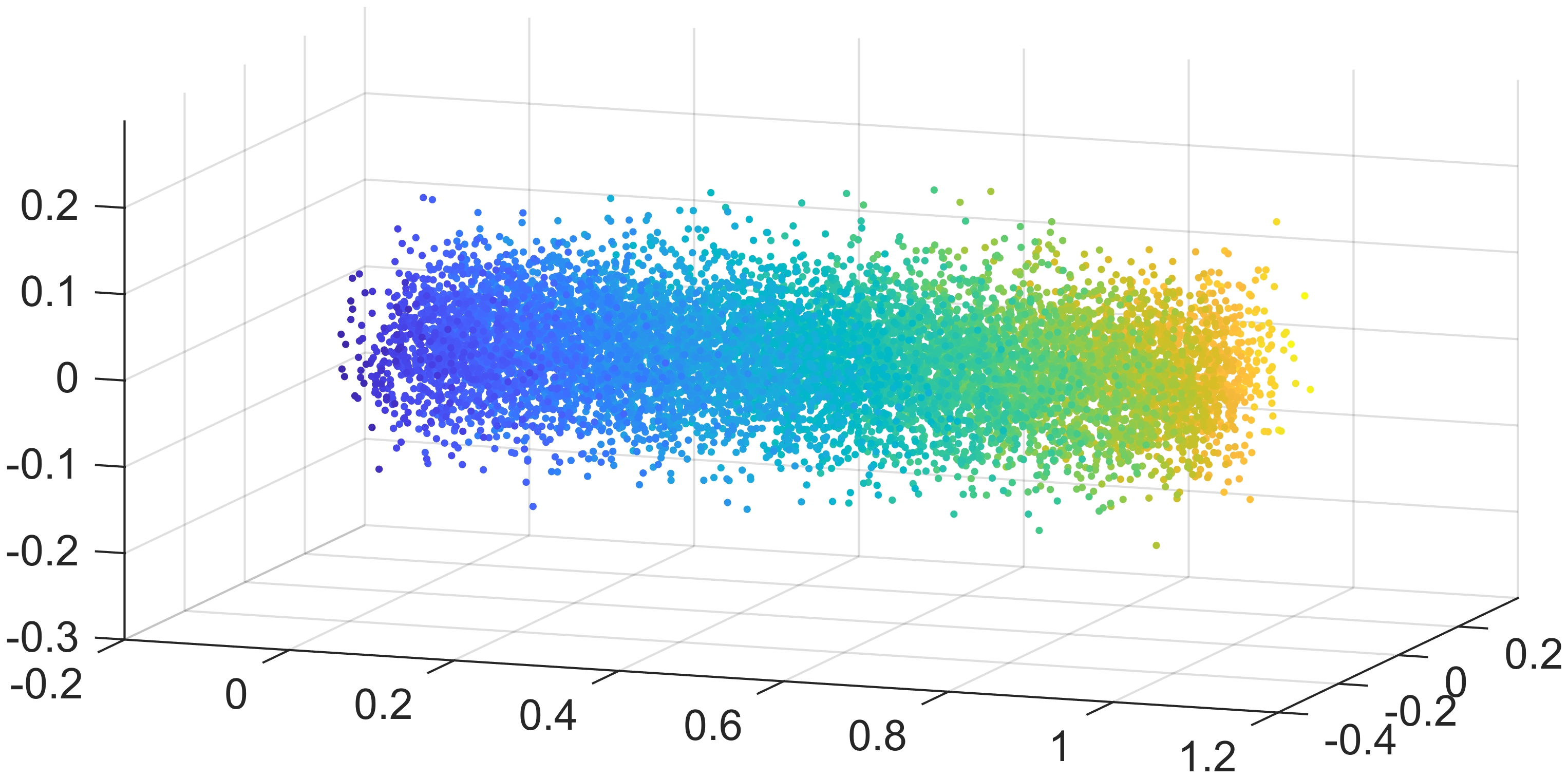
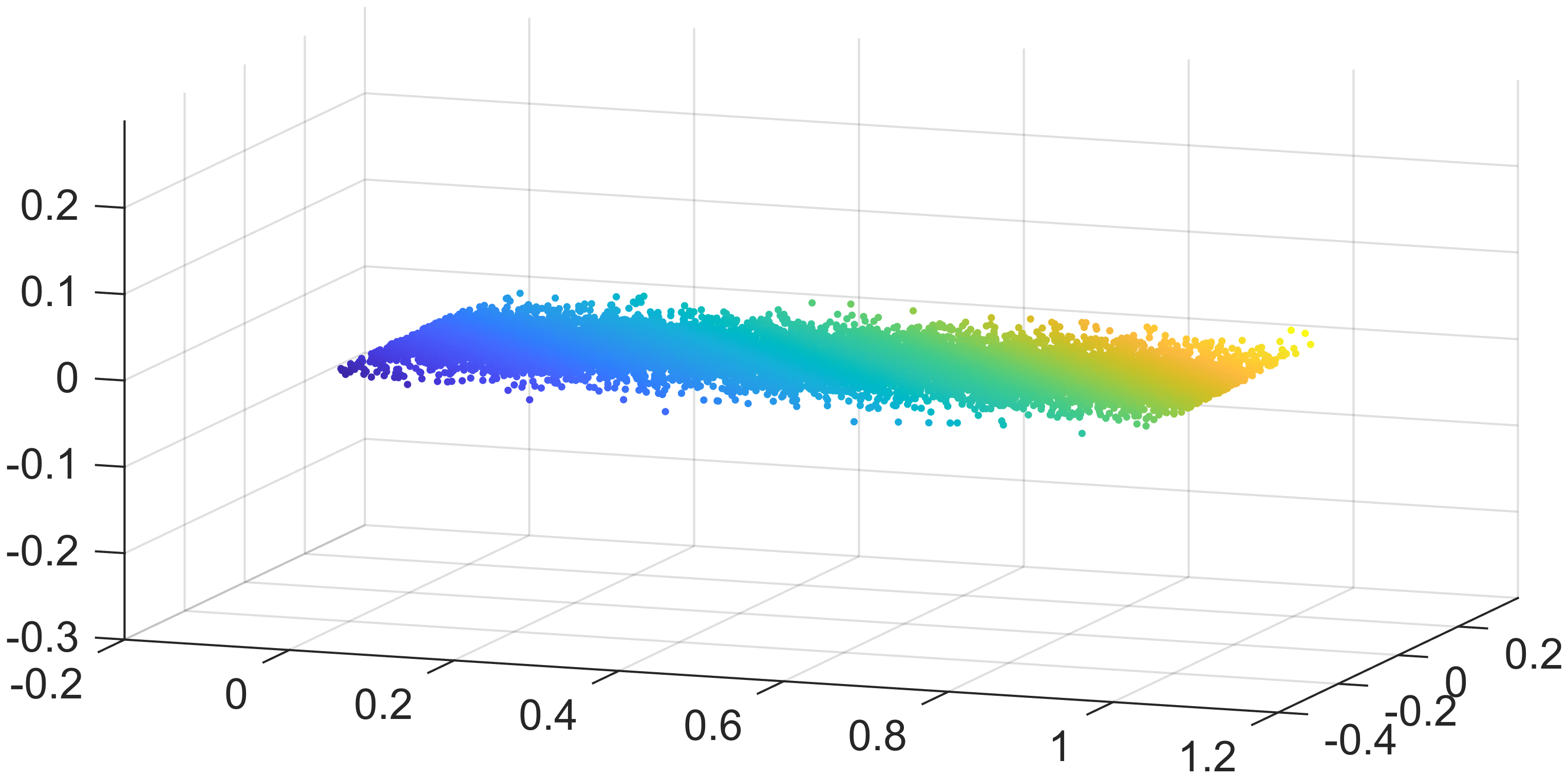
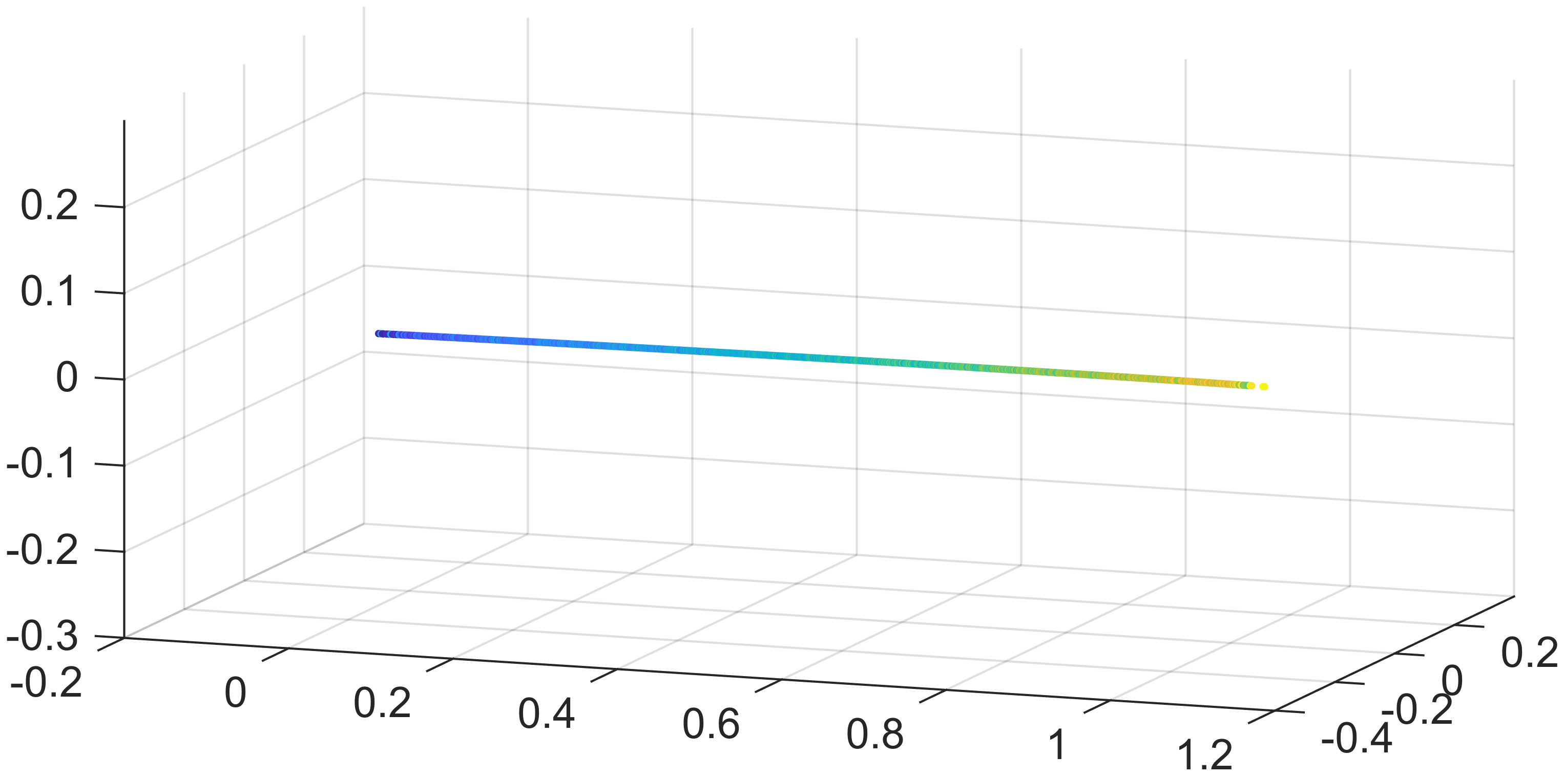
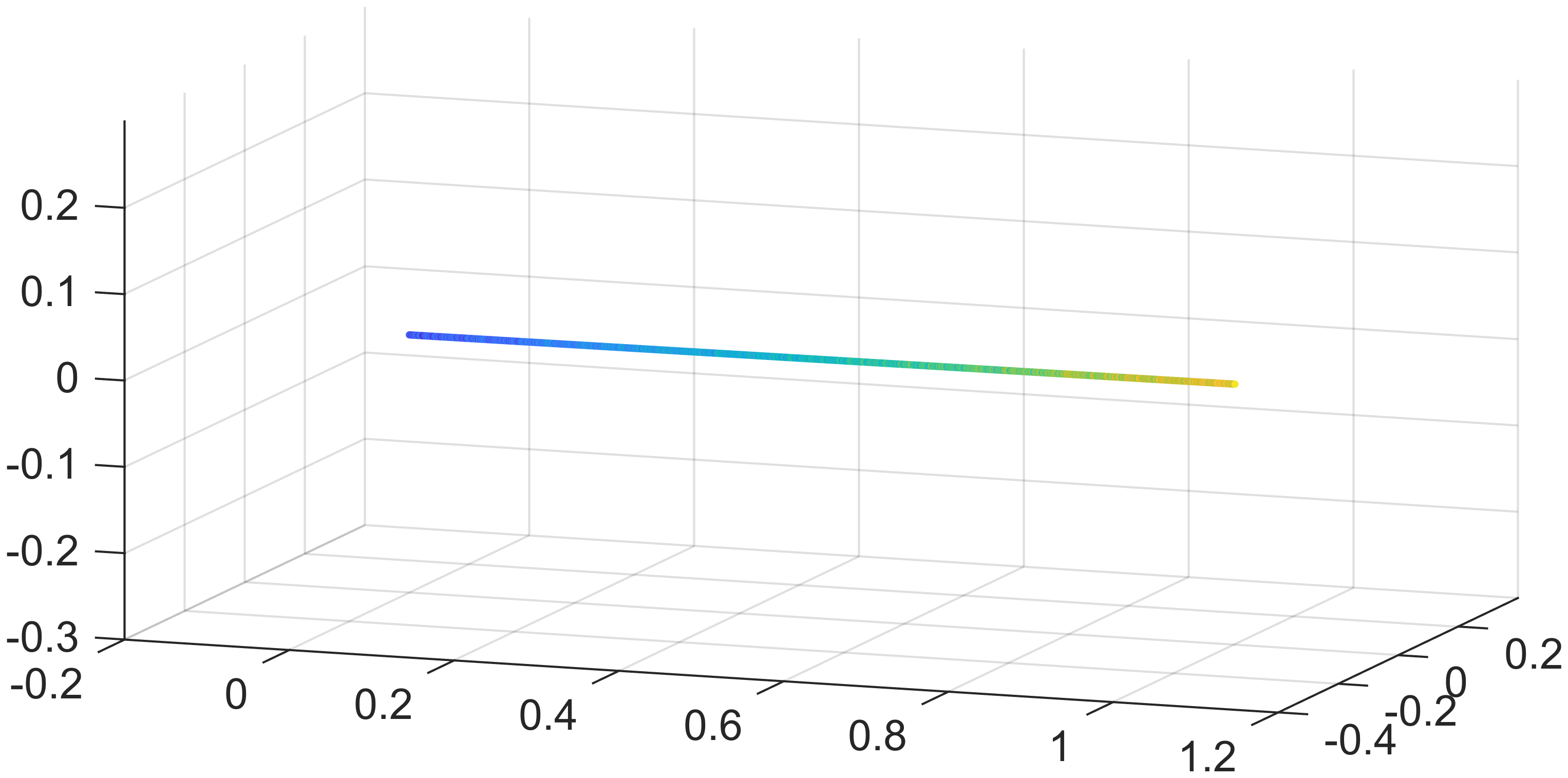
Figure 3: Scatter plots for the line segment case in $\mathbb{R}^{3}$ with colors added to enhance the visualization of sample adjacency. (a) Input data set; (b,c) Projection results onto the principal nested submanifolds of dimensions 2 and 1, respectively; (d,e) Projections onto the first two and single principal components, respectively.

Figure 3 presents the input data and projection results from the two methods. The points projected with our method are shown in Figure 3 and Figure 3, where the points lie very close to the xy-plane and x-axis, respectively. This demonstrates that the proposed method successfully handles the scenario with identifiable fixed principal directions and approximates the linear subspaces effectively. The projection results are remarkably similar to those obtained from principal component analysis, as illustrated in Figure 3 and Figure 3. This similarity indicates that our method performs comparably well even in the linearly generated scenarios.

Subsequently, we introduce nonlinearity into the generatring curve. Consider the unit circle

$$\gamma_{2}(t)=\bigl{(}\cos(t),\sin(t),0\bigl{)}^{\top},~t\in(0,1),$$

where $n=10^{4}$ points are sampled, and noise is introduced in the directions $v_{1}=(0,0,1)^{\top}$ and $v_{2}=(\cos(t),\sin(t),0)^{\top}$, with standard deviations $\sigma_{1}=0.1$ and $\sigma_{2}=0.05$, respectively. The resulting data set, shown in Figure 4, resembles a torus that is thicker in the z-axis direction.

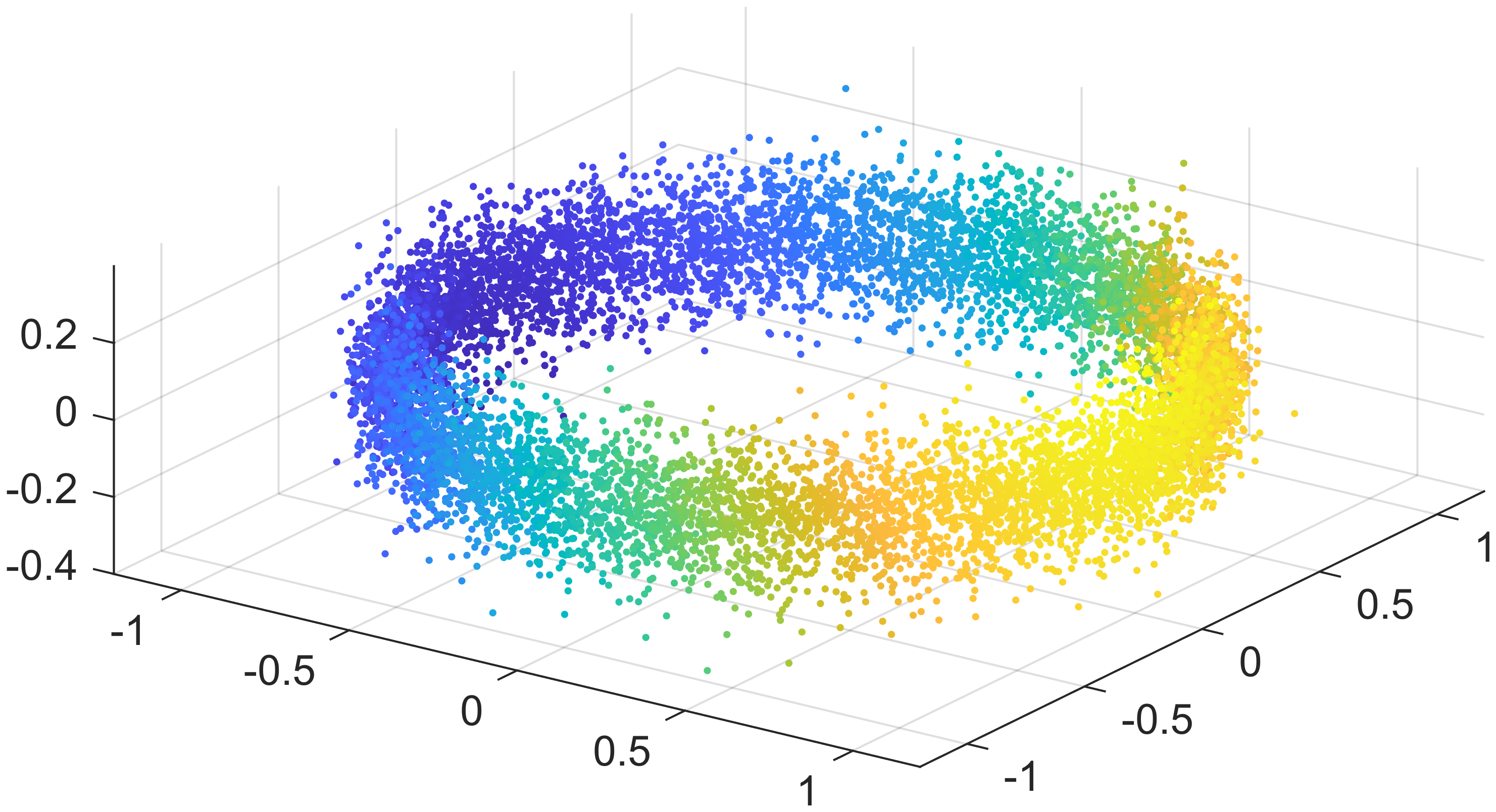
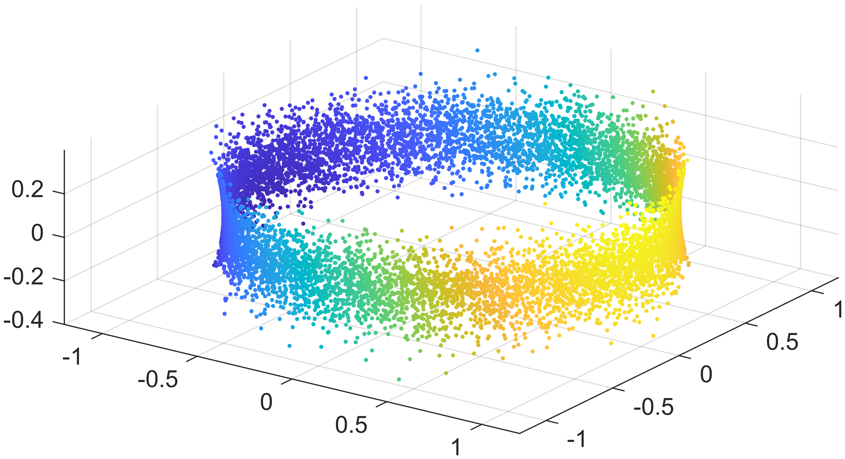
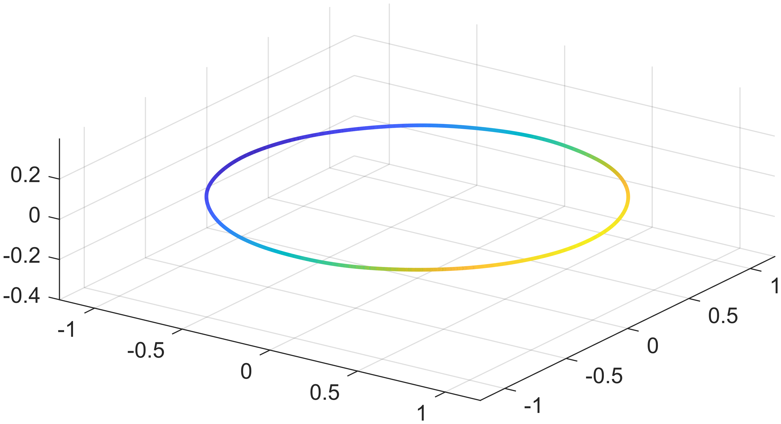
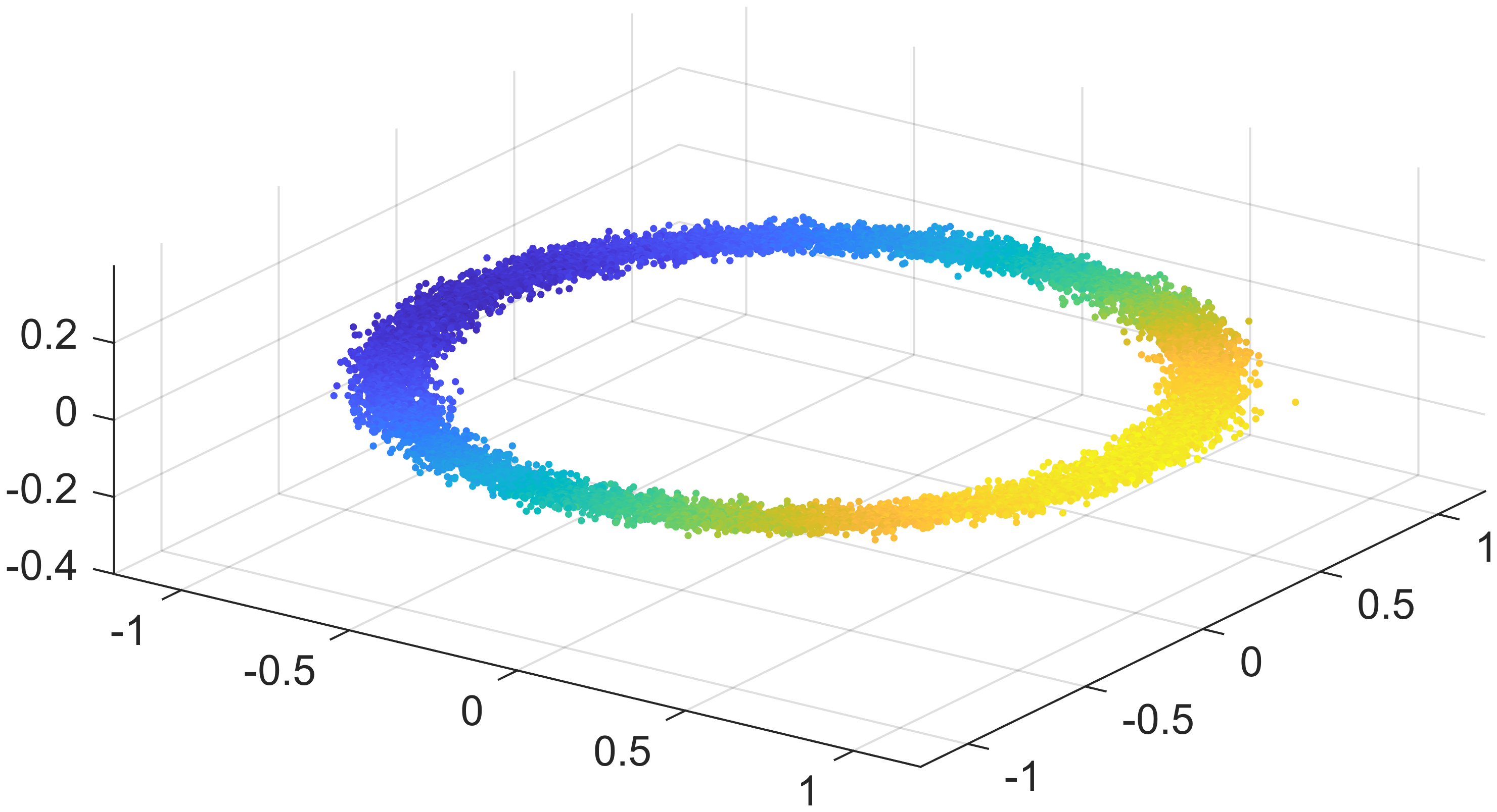
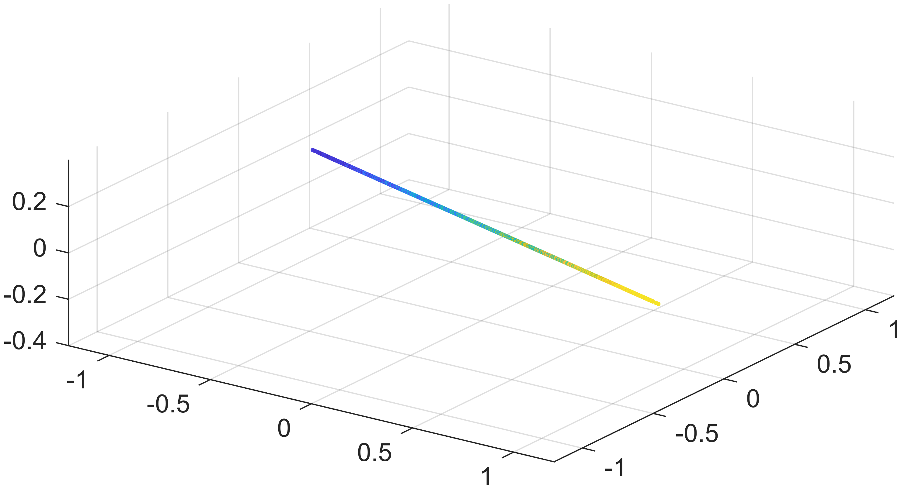
Figure 4: Scatter plots for the circle case in $\mathbb{R}^{3}$ with colors added to enhance the visualization of sample adjacency. (a) Input data set; (b,c) Projection results onto the principal nested submanifolds of dimensions 2 and 1, respectively; (d,e) Projections onto the first two and single principal components, respectively.

The input data and projection results from the two methods are visualized in Figure 4. Figure 4 presents the two dimensional projection with our method, which is a circular strip with width in the z-axis direction. This suggests that our method successfully fits a two-dimensional submanifold that captures the majority of variation in $\mathcal{X}_{n}$ by removing the variation along the smallest principal direction. In contrast, the 2-dimensional projection with principal component analysis, as shown in Figure 4, is an annulus approximately on the xy-plane. This indicates that the principal component analysis primarily focuses on the global covariance structure and overlooks the local principal direction corresponding to the smallest eigenvalue. These points are further projected on one-dimensional structures, and the results are present in Figure 4 and Figure 4. It is clear that our method is able to recover the circle structure of $\gamma_{2}$ while principal component analysis fails due to its focus on linear subspace.

Finally, we consider a more complex correlation structure. Let the generating curve be

$$\gamma_{3}(t)=\left(\frac{t}{6}\cos(t),~\frac{t}{6}\sin(t),~\frac{t}{6}\right)^{\top},\quad t\in(0,6\pi),$$

where $n=10^{4}$ random points are generated. At point $\gamma_{3}(t)$, consider an orthonormal basis

$$v_{T}=\frac{\dot{\gamma_{3}}(t)}{\|\dot{\gamma_{3}}(t)\|},\quad v_{N}=\frac{\ddot{\gamma_{3}}(t)}{\|\ddot{\gamma_{3}}(t)\|},\quad v_{B}=\frac{v_{T}\times v_{N}}{\left\|v_{T}\times v_{N}\right\|}.$$

Noise with standard deviations $\sigma_{1}=0.09$ and $\sigma_{2}=0.03$ is introduced in the directions

$$v_{1}=\sin(2t)v_{B}+\cos(2t)v_{N}~\text{ and }~v_{2}=\cos(2t)v_{B}-\sin(2t)v_{N},$$

respectively. The resulting data set, shown in Figure 5, can be regarded as the region swept by a rotating ellipse whose center translates along $\gamma_{3}$.

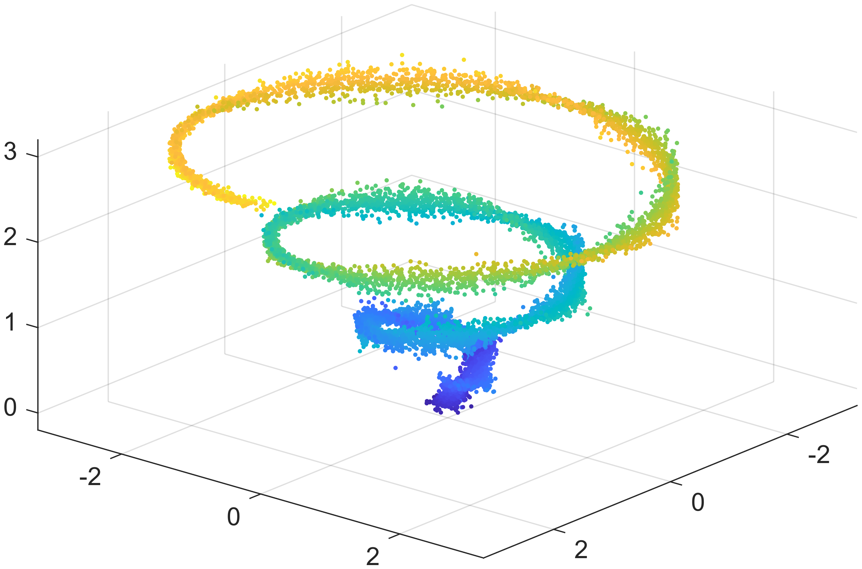
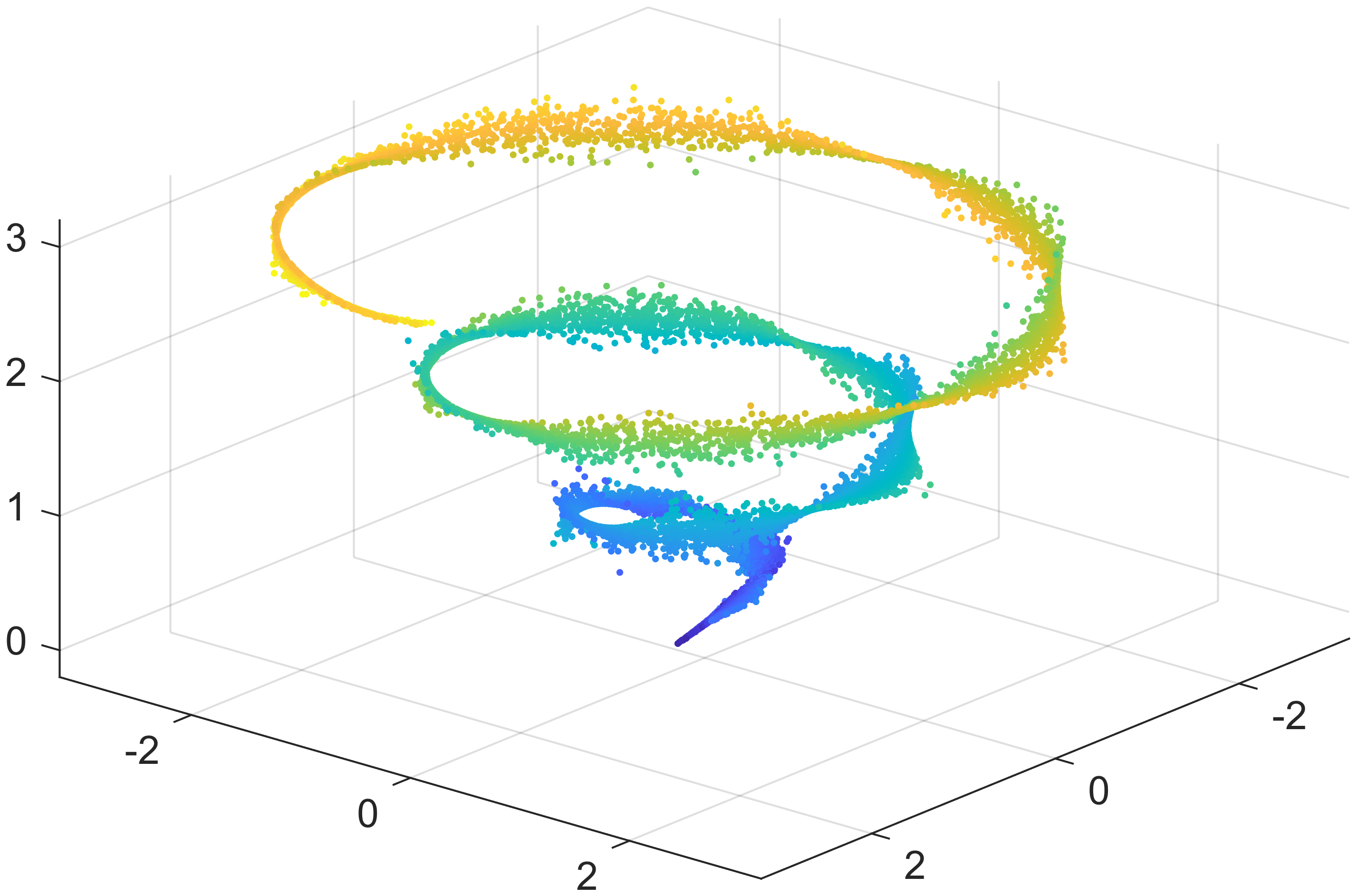
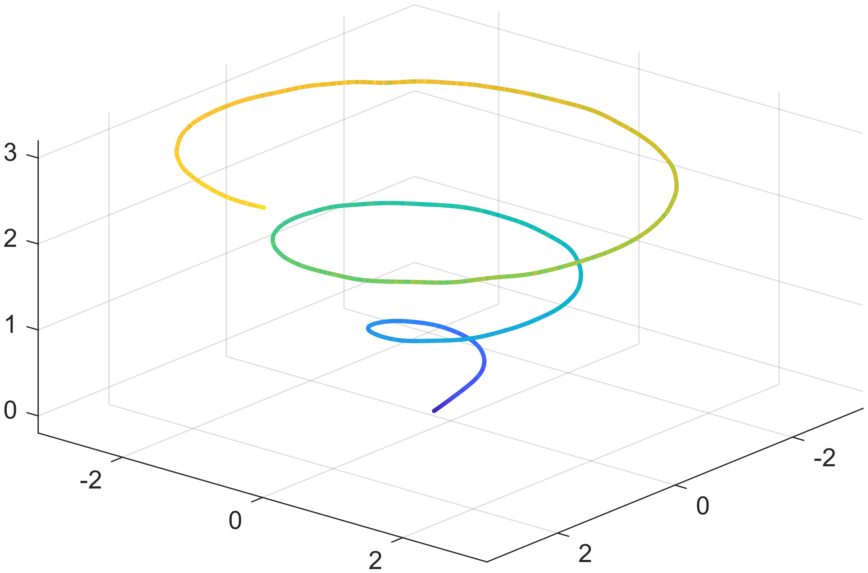
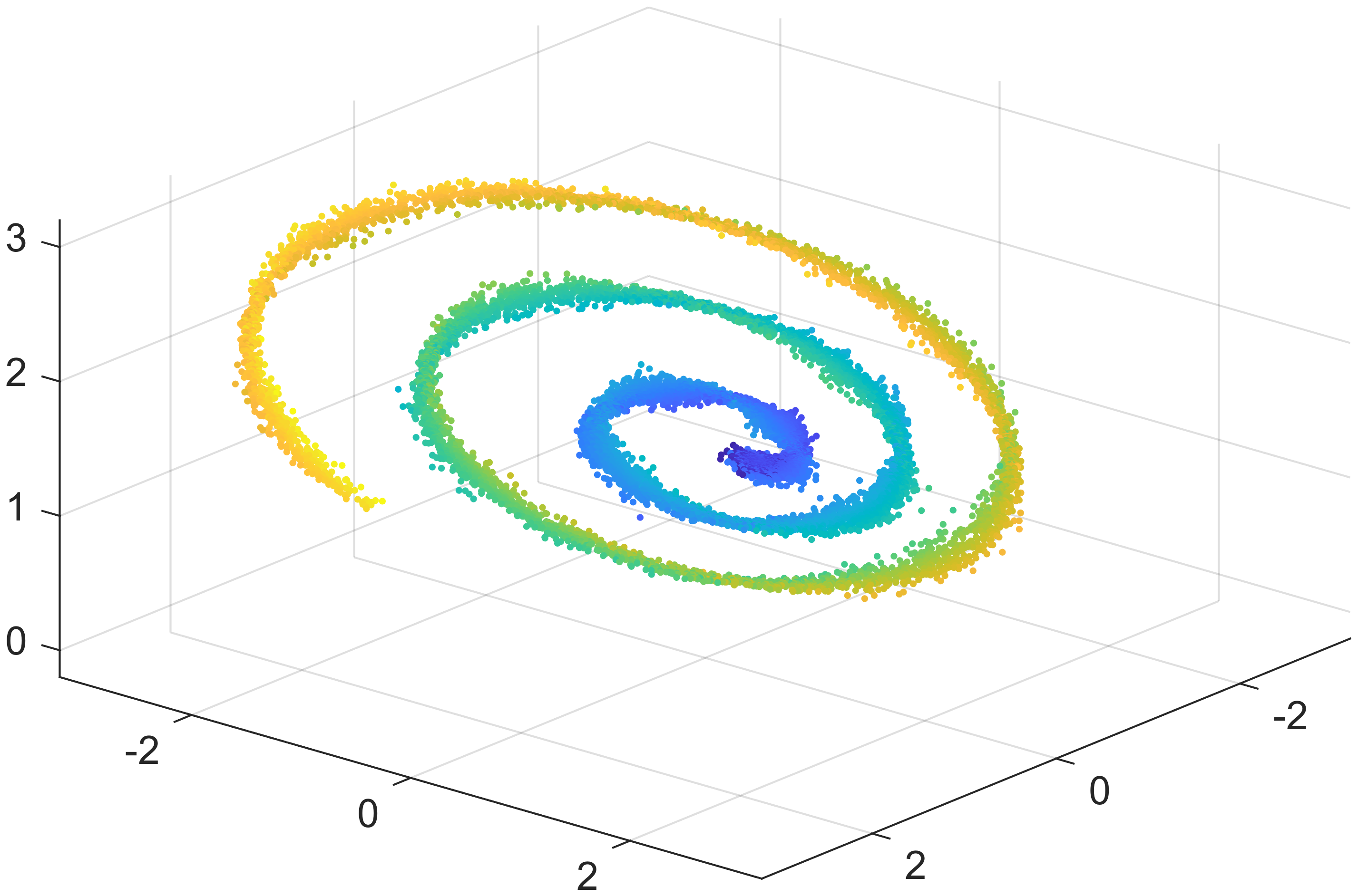
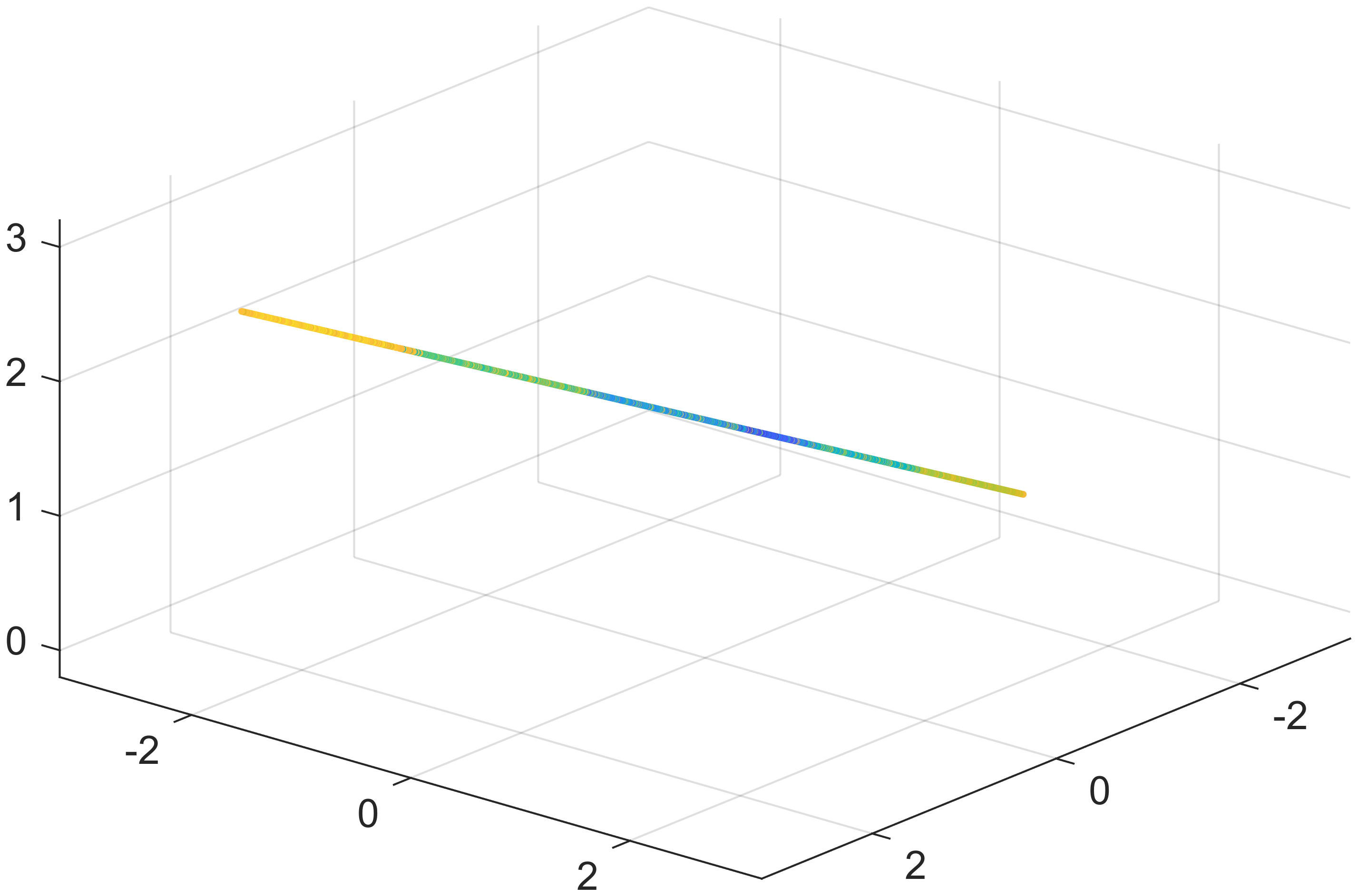
Figure 5: Scatter plots for the involute case in $\mathbb{R}^{3}$ with colors added to enhance the visualization of sample adjacency. (a) Input data set; (b,c) Projection results onto the principal nested submanifolds of dimensions 2 and 1, respectively; (d,e) Projections onto the first two and single principal components, respectively.

Figure 5 presents the input data and projection results from the two methods. The two-dimensional projection with our method is shown in Figure 5, which is a rotating strip along the involute with the surface suits the direction of $v_{T}$ and $v_{1}$. This result suggests that our method is still able to capture the covariance structure in the form of smooth functions and fit low-dimension structure by removing variation along the principal direction corresponding to the smallest eigenvalue. In contrast, as shown in Figure 5, principal component analysis projects the points by flattening the point cloud onto a plane, which loses too much details of the structure. These points are further projected on one-dimensional subspaces, and the results are present in Figure 5 and Figure 5. It is evident that our method is able to recover the involute structure from $\mathcal{X}_{n}$, whereas principal component analysis fails due to its linearity restriction.

Overall, our method is effective in dealing with data around low-dimensional structures in Euclidean space in terms of decomposition and dimension reduction. This is achieved by adaptively exploiting the local sample covariance structure and combining it with the manifold fitting approach. In contrast, while principal component analysis is able to project samples into nested low-dimensional subspaces, its inherent linearity limits its ability to dynamically exploit the covariance structure. As a result, it performs suboptimal when sample correlations are nonlinear.

4.2 Simulation in shape spaces

In this subsection, we explore the decomposition of sample points around low-dimensional structures in shape spaces like spheres and tori, comparing our proposed method with the principal nested spheres and the torus principal component analysis in different cases. We still consider a generating curve $\{\gamma(t)\mid t\in\mathcal{T}\}\subset[0,2\pi]^{2}$ and uniformly generate $n$ sample points $\{t_{i}\}_{i=1}^{n}\subset\mathcal{T}$ in each case. Next, we introduce noise in the normal direction of $\gamma$ in $[0,2\pi]^{2}$. Specifically, a noisy angle pair in the angle plane is given by

$$(\phi_{i},\psi_{i})^{\top}=\gamma(t_{i})+\xi_{i}\frac{\ddot{\gamma}(t_{i})}{\|\ddot{\gamma}(t_{i})\|},\quad i=1,\dots,n,$$ (4)

where $\{\xi_{i}\}_{i=1}^{n}$ denotes a set of independent and identically distributed random noise amplitudes, each drawn from a normal distribution, $\mathcal{N}(0,0.1^{2})$. Given that scaling the entire sample set does not influence the analysis, we embed these angles onto $\mathcal{S}^{2}$ and $T^{2}=\mathcal{S}^{1}\times\mathcal{S}^{1}$ respectively, which leads to the manifold-valued sample set $\mathcal{X}_{n}$. This embedding results in a locally two-dimensional subset within the shape space. We then apply our proposed method, using a radius $r=0.5$, to $\mathcal{X}_{n}$ to project it onto the one-dimensional principal nested submanifolds. For comparative analysis, we perform both the principal nested spheres and torus principal component analyses.

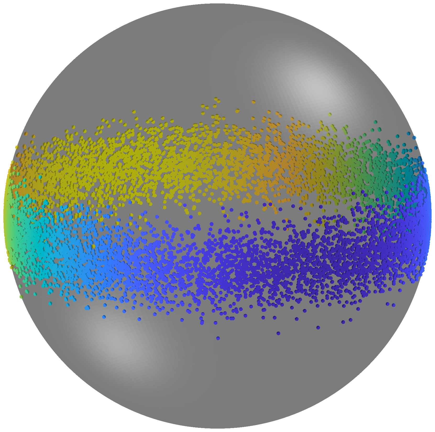
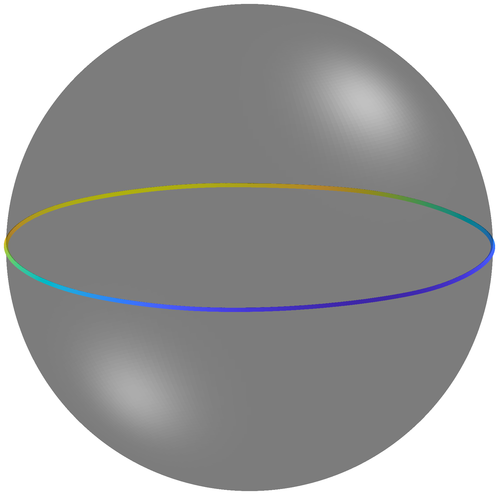
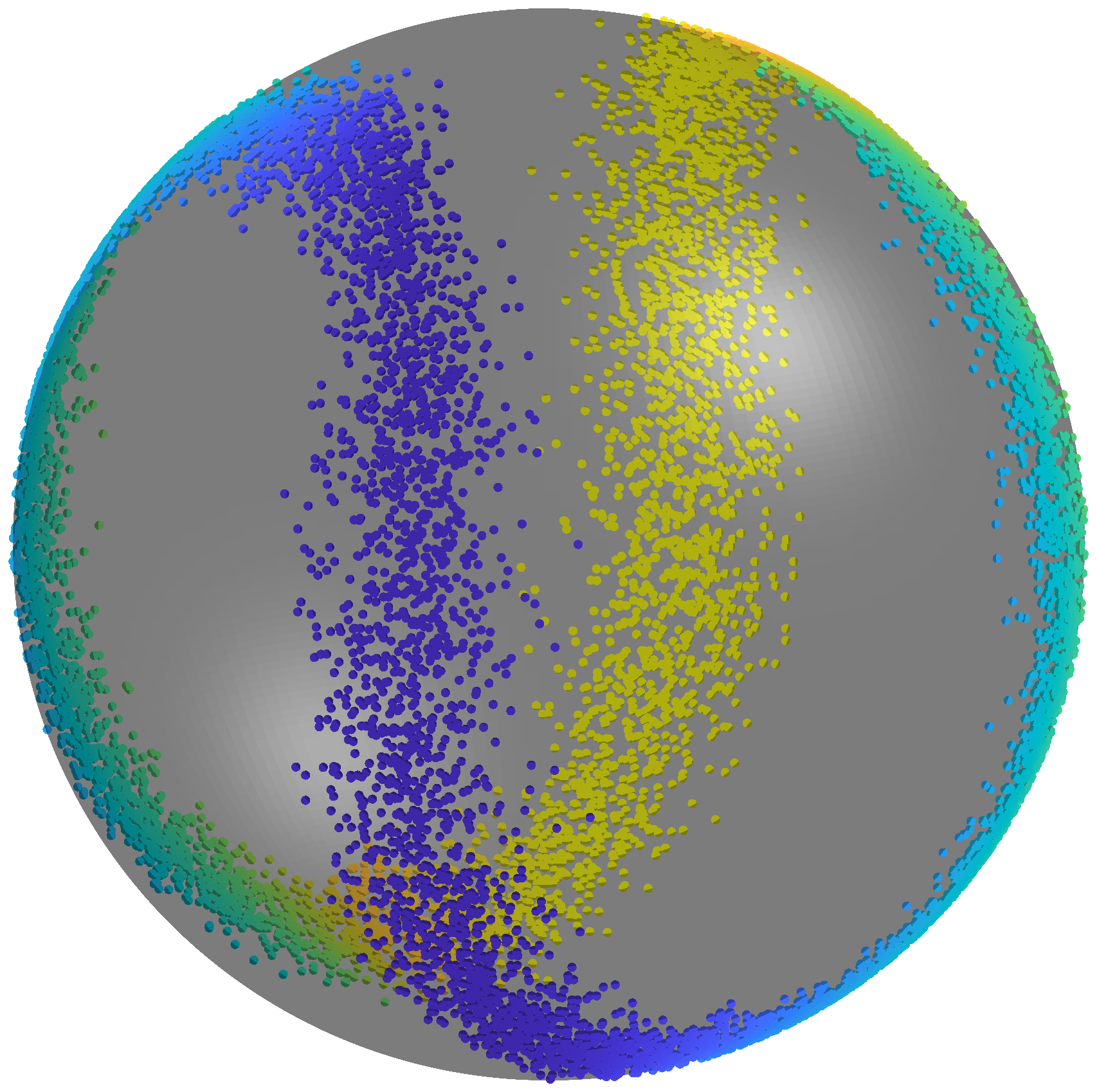
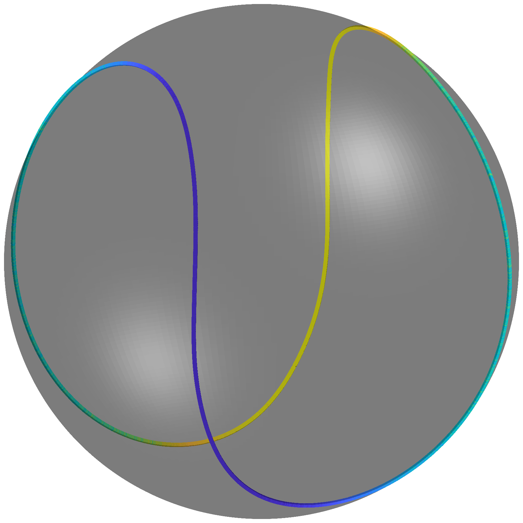
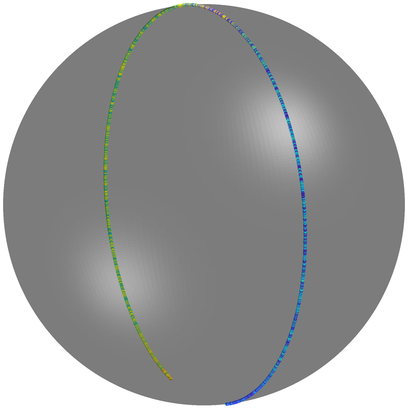
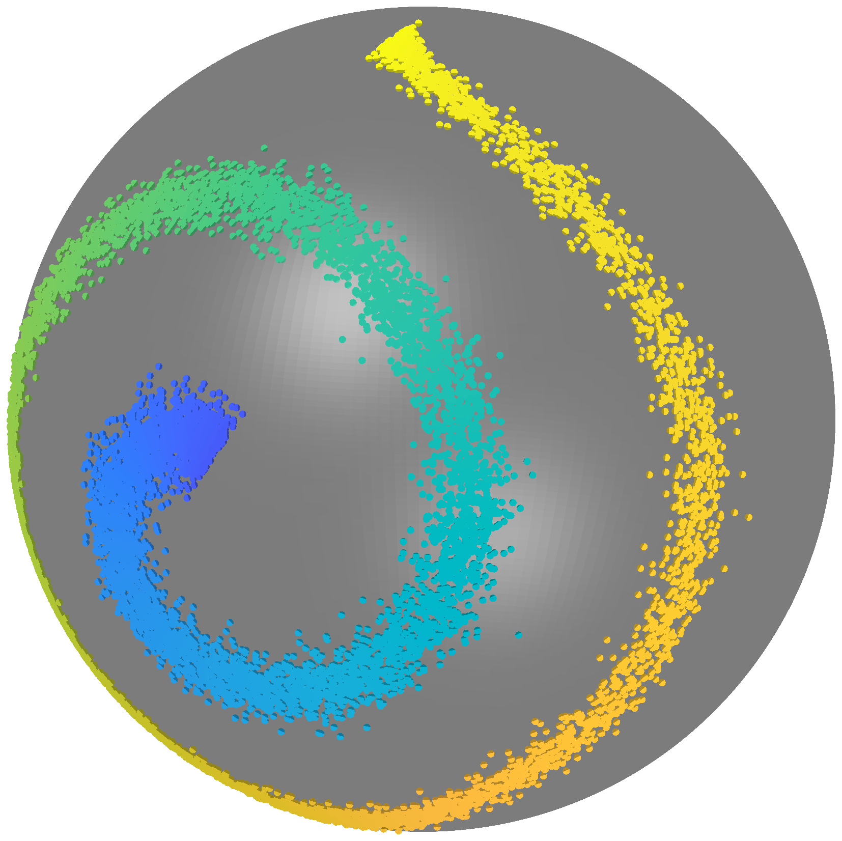
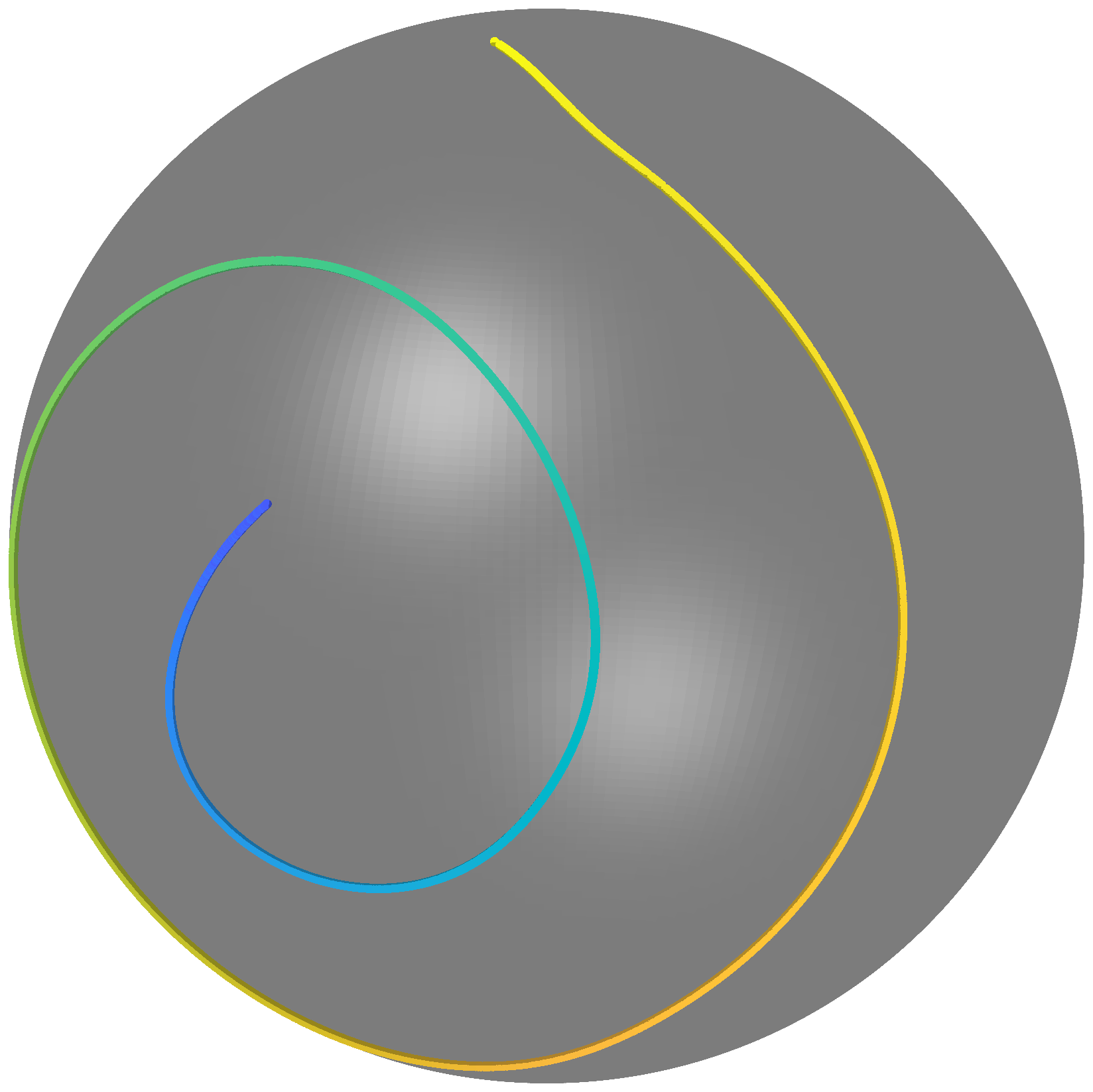
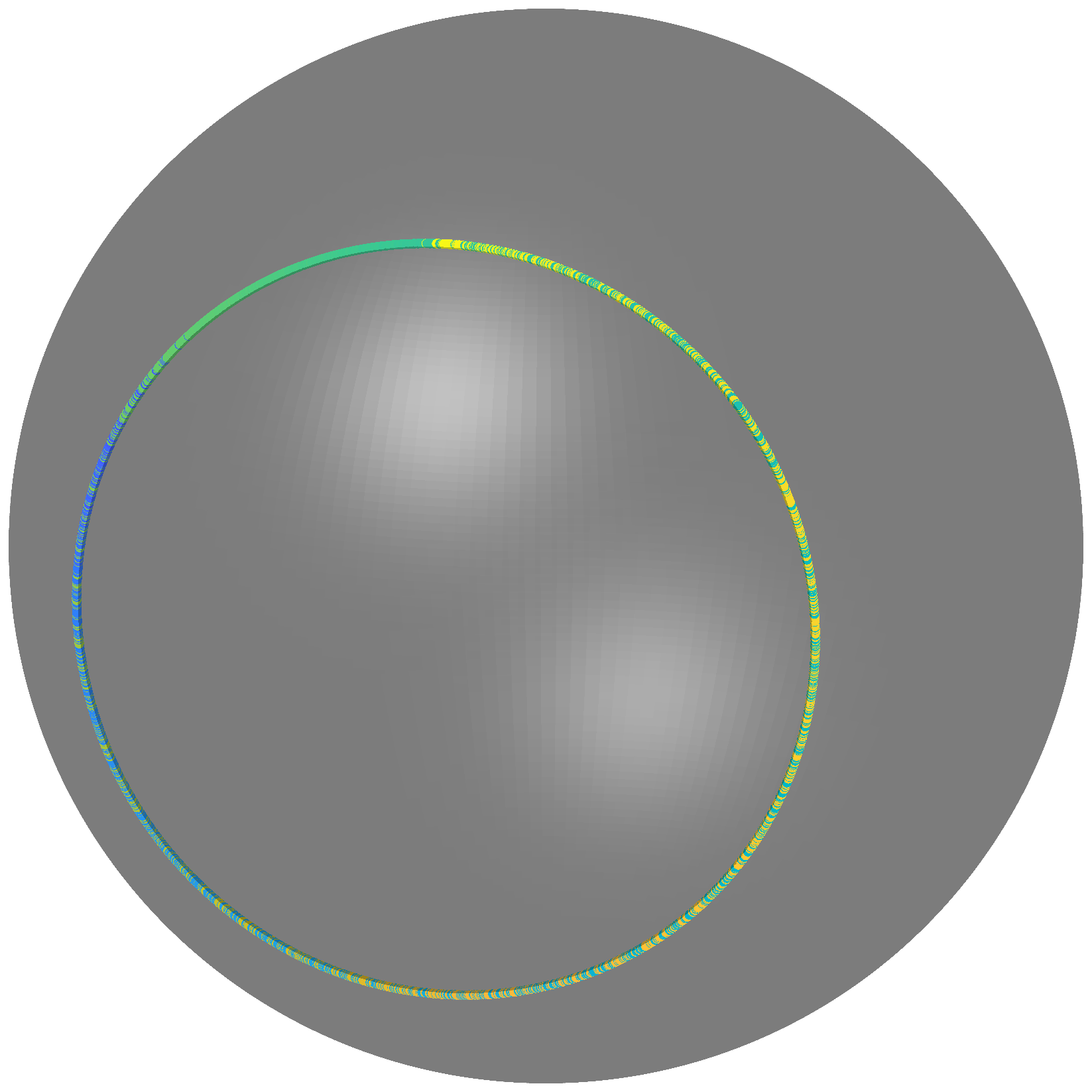
Figure 6: Scatter plots for the sphere case with colors added to enhance the visualization of sample adjacency. Each row corresponds to one generative curve. The left column panels display the input data; the middle panels show the results with principal nested submanifolds, and the right column presents the results from principal nested spheres.

First, we investigate the decomposition of the data on spheres. In this case, samples are generated with three curves

$$\gamma_{1}(t) =\left(t,0\right)^{\top},\quad t\in(0,2\pi);$$

$$\gamma_{2}(t) =\begin{cases}\left(\arctan\left\{\tan^{3}(t)-\frac{\pi}{2}\right\},\arccos\left\{\surd 3\sin(t)\cos(t)\right\}\right)^{\top},&t\in(0,\pi),\\ \left(\arctan\left\{\tan^{3}(t)+\frac{\pi}{2}\right\},\arccos\left\{\surd 3\sin(t)\cos(t)\right\}\right)^{\top},&t\in(\pi,2\pi);\\ \end{cases}$$

$$\gamma_{3}(t) =\left(\frac{t}{10}\cos(t),\frac{t}{10}\sin(t)\right)^{\top},\quad t\in\left(\frac{\pi}{2},\frac{9\pi}{2}\right).$$

with the data generating function in (4), a set of $n=10^{4}$ noisy angle pairs in the angle plane for each case, and these angle pairs are embedded into a unit sphere $\mathcal{S}^{2}\subset\mathbb{R}^{3}$ by

$$x_{i}=\bigl{(}\cos(\psi_{i})\cos(\phi_{i}),~\cos(\psi_{i})\sin(\phi_{i}),~\sin(\psi_{i})\bigl{)}^{\top},\quad i=1,\dots,n.$$

The resulting data sets are shown in the left-most column of Figure 6, which resemble a circle, a tennis curve, and an involute on $\mathcal{S}^{2}$ respectively. Then, the proposed method and the principal nested spheres are applied to these data to project them on one-dimensional submanifolds of $\mathcal{S}^{2}$.

The middle column of Figure 6 presents the projection results of our method. In each case, the points projected by our method are approximately on a curve that passes through the center of the sample, and the neighbourhood relationship between the samples is well maintained. This suggests that our method can fit submanifolds on spheres to explain the majority of sample variation. In contrast to our approach, the principal nested spheres can only projects the samples on circles cut from the sphere, as shown in the last column of Figure 6, which leads to the loss in neighbourhood information. This drawback is similar to principal component analysis, which comes from the restriction of subspaces, but our method is not constrained in this way.

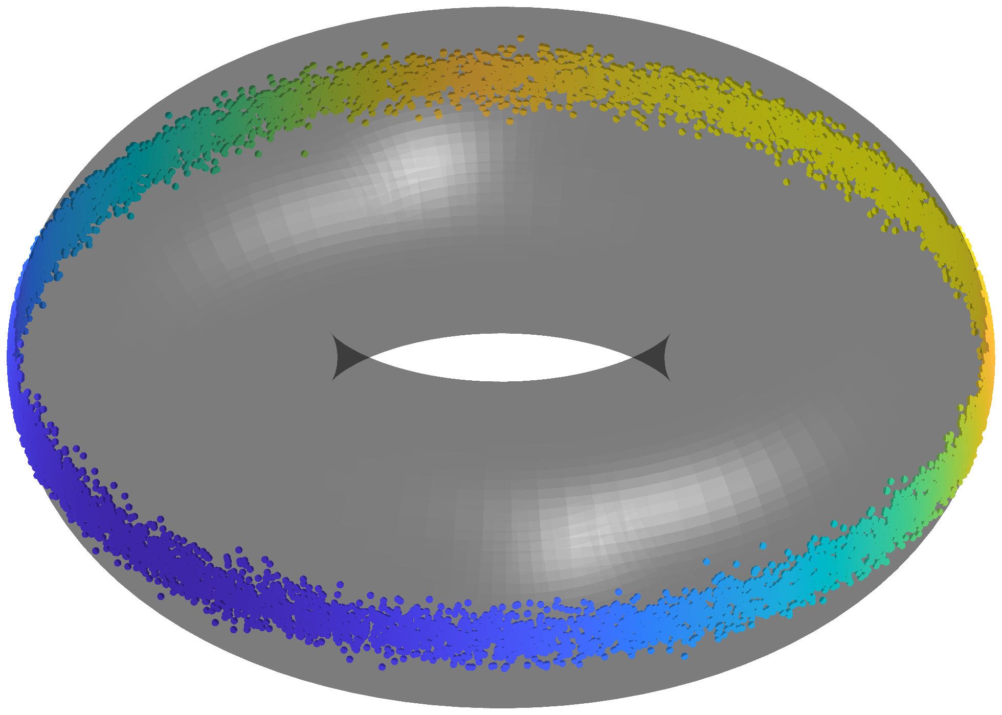
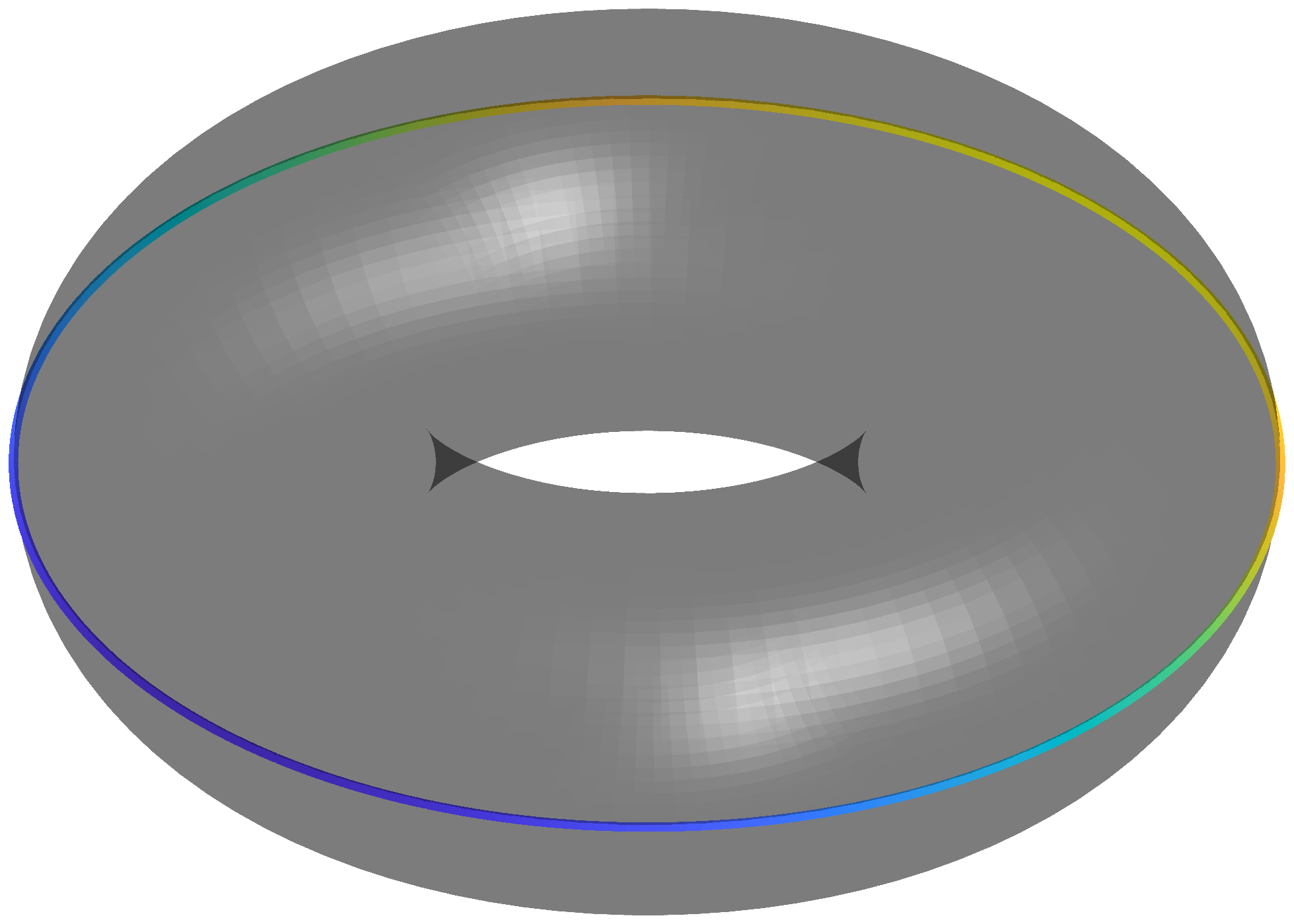
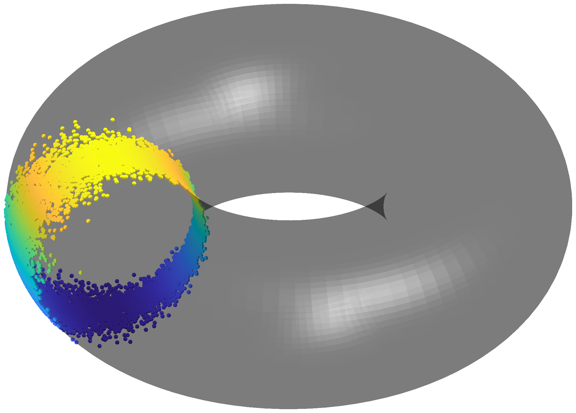
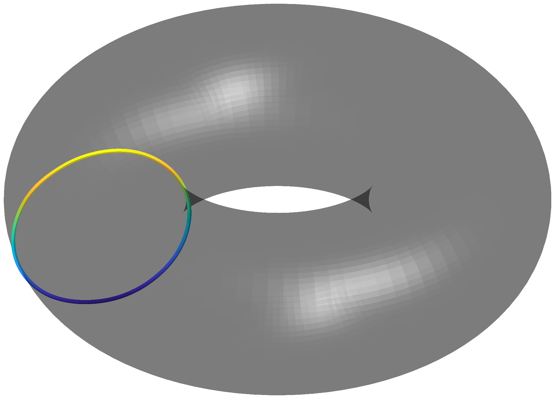
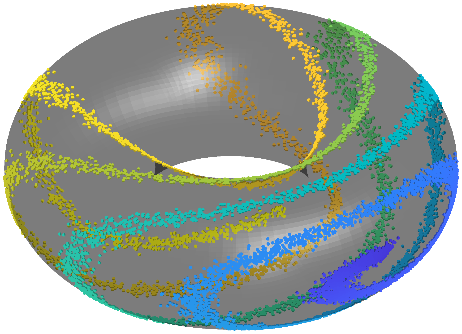
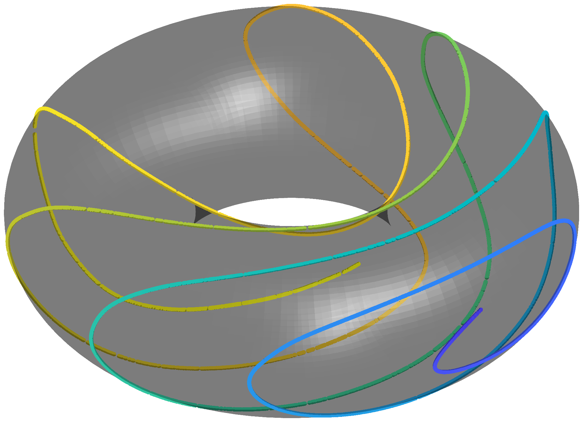
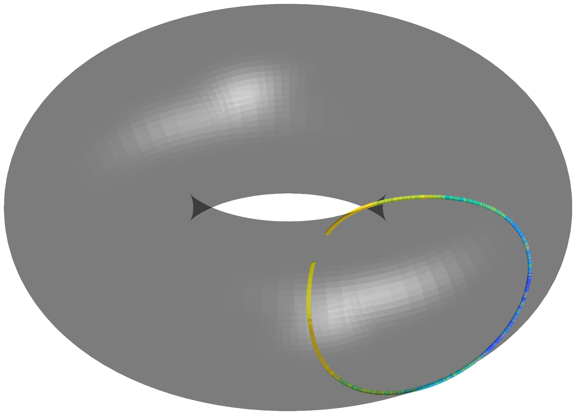
Figure 7: Scatter plots for the torus case with colors added to enhance the visualization of sample adjacency. Each row corresponds to one generative curve. The left column panels display the input data; the middle panels show the results with principal nested submanifolds, and the right column presents the results from the torus principal component analysis.

Then, we investigate the decomposition of the data on torus. In this case, samples are generated with three curves

$$\gamma_{1}(t) =\left(t,0\right)^{\top},\quad t\in(0,2\pi);$$

$$\gamma_{2}(t) =\left(-2\pi/3,t\right)^{\top},\quad t\in(0,2\pi);$$

$$\gamma_{3}(t) =\left(\frac{t}{10}\cos(t),~\frac{t}{10}\sin(t)\right)^{\top},\quad t\in\left(\frac{\pi}{2},\frac{19\pi}{2}\right),$$

with the data generating function in (4), a set of $n=10^{4}$ noisy angle pairs in the angle plane for each case, and these angle pairs are embedded into a torus in $\mathbb{R}^{4}$ by

$$x_{i}=\bigl{(}\cos(\phi),~\sin(\phi),~\cos(\psi),~\sin(\psi)\bigl{)}^{\top},\quad i=1,\dots,n.$$

For better visualization, all the results are transformed back to the angles and further embedded in a torus in $\mathbb{R}^{3}$ by

$$(\phi,\psi)\mapsto\bigl{(}\{1+0.5\cos(\psi)\}\cos(\phi),~\{1+0.5\cos(\psi)\}\sin(\phi),~0.5\sin(\psi)\bigl{)}^{\top}.$$

The resulting data sets are shown in the left-most column of Figure 7, which resemble two circles and an involute on the torus respectively. Then, the proposed method is applied to these data sets in $\mathbb{R}^{4}$ to project them on a one-dimensional submanifold while the torus principal component analysis is directly applied on the angle pairs.

The projection results of our method are shown in the middle column of Figure 7. In each case, the points projected by our method are approximately on a curve that passes through the center of the sample, and the neighbourhood relationship between the samples is well maintained. This suggests that our method can fit submanifolds on torus to explain the majority of sample variation. In contrast to our approach, the torus principal component analysis only projects the samples on circles cut from the torus, as shown in the last column of Figure 7, which mixes up points from different regions of the sample. This flaw is also inherited from principal component analysis and the principal nested spheres, and our method is again not plagued by this on torus.

In summary, our method effectively decomposes and performs dimension reduction on data around low-dimensional structures in spheres and tori. This is achieved by adaptively exploiting the local sample covariance structure and using manifold fitting methods. In contrast, methods like principal nested spheres and torus principal component analysis, which also project samples onto subspaces of specific dimensions, impose restrictions on the form of subspaces. This often results in the mixing of samples from different parts, leading to suboptimal decomposition outcomes.

5 Application to single-cell RNA sequencing data

In this section, we investigate the application of the proposed method to the single-cell RNA-sequencing data set reported by Haber et al. (2017). This data set originates from the small intestinal epithelium of six mice. The processing of the samples is detailed in (Haber et al., 2017). In summary, the epithelium tissues undergo cell isolation, crypt isolation, cell sorting, and RNA sequencing, resulting in an expression matrix of 7,216 cells across 15,971 genes. The data is preprocessed by removing lowly expressed genes from individual cells and performing dimension reduction on highly expressed genes with principal component analysis following a logarithmic transformation. The 13 significant components are then used to construct a 200-nearest-neighbour graph, which serves as the input for Infomap (Rosvall and Bergstrom, 2008). This process clusters the cells into 15 biologically significant groups (see Table 1 for these groups). Our analysis will concentrate on the 13 significant components, using the 15 cell types as labels.

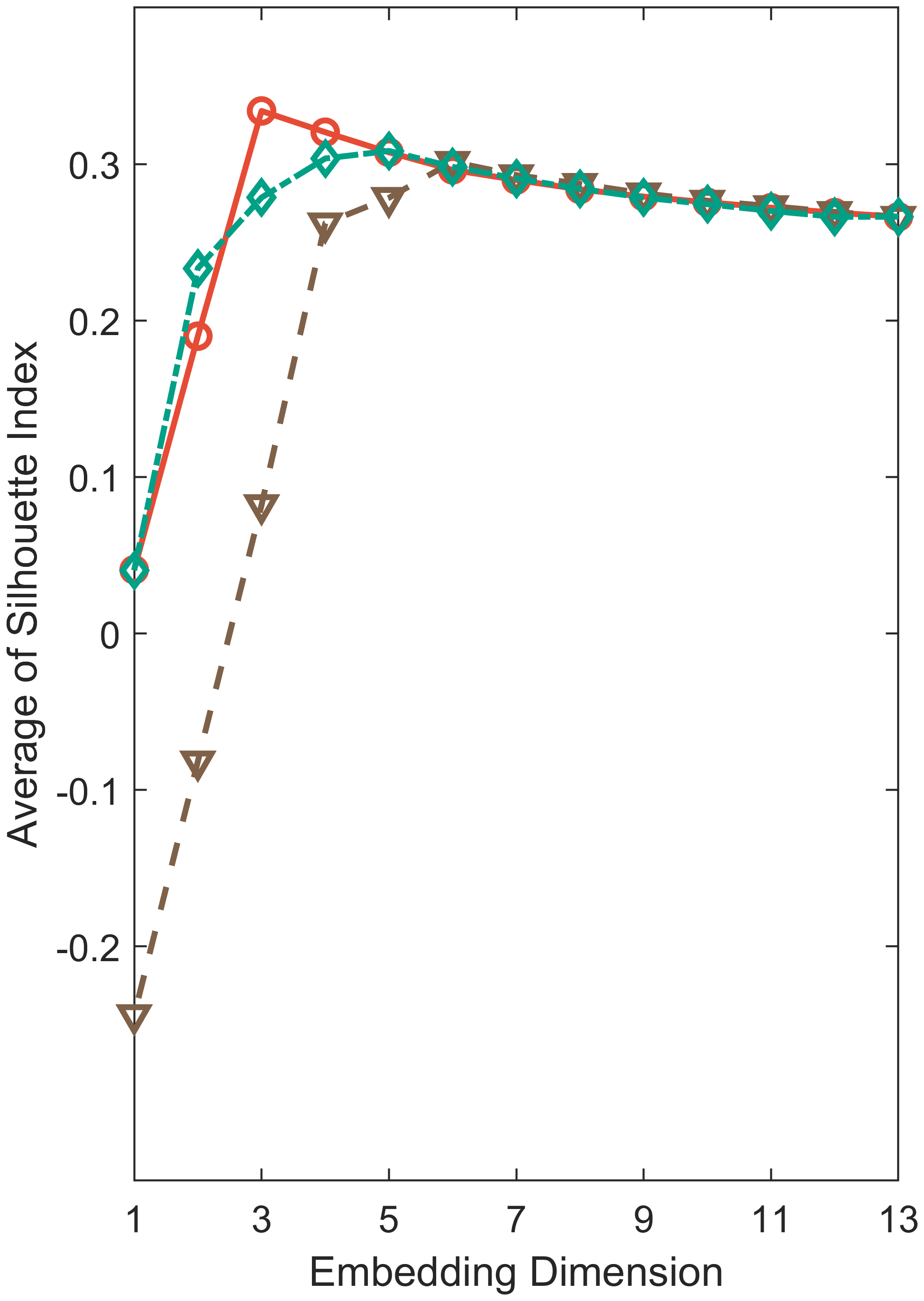
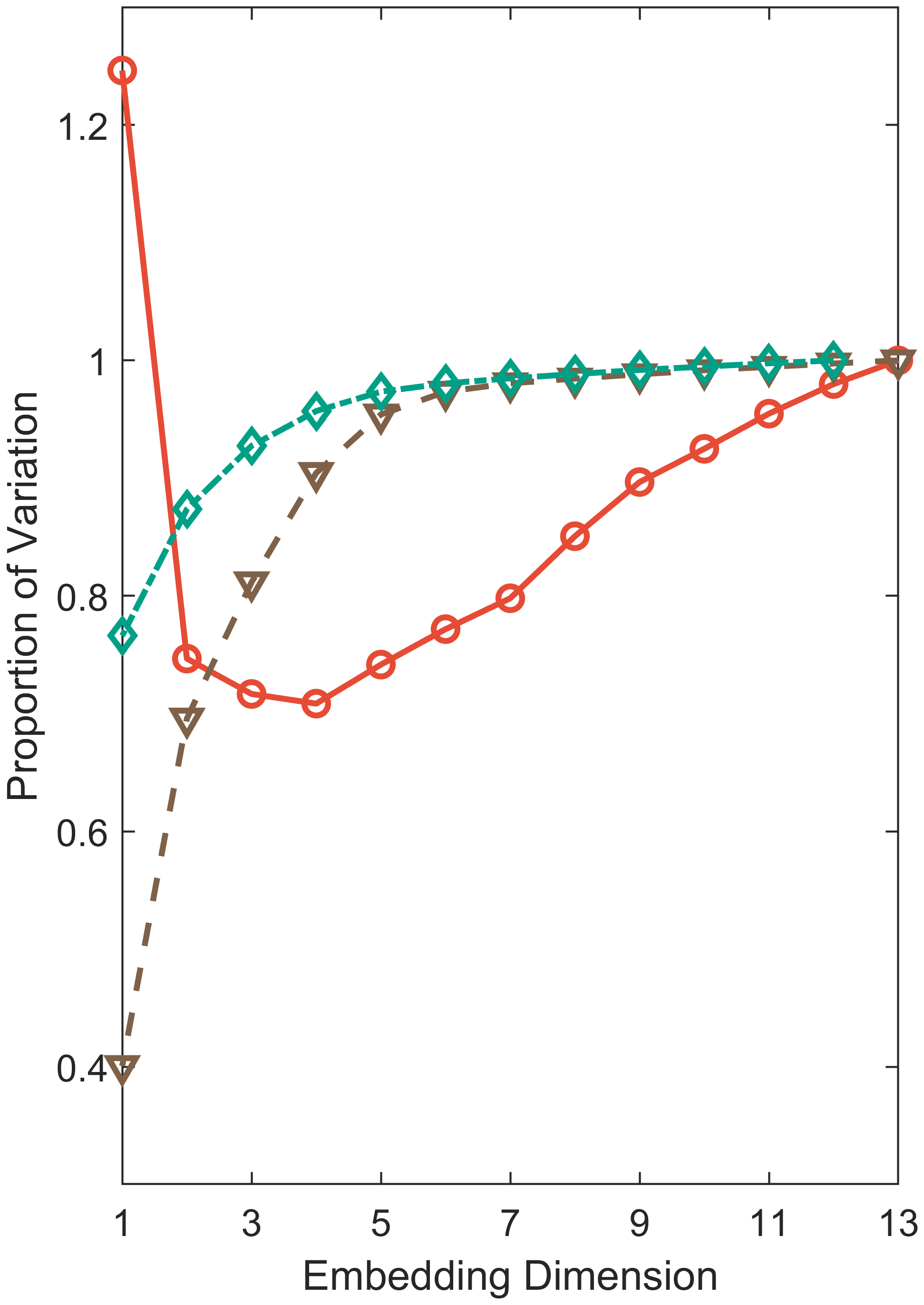
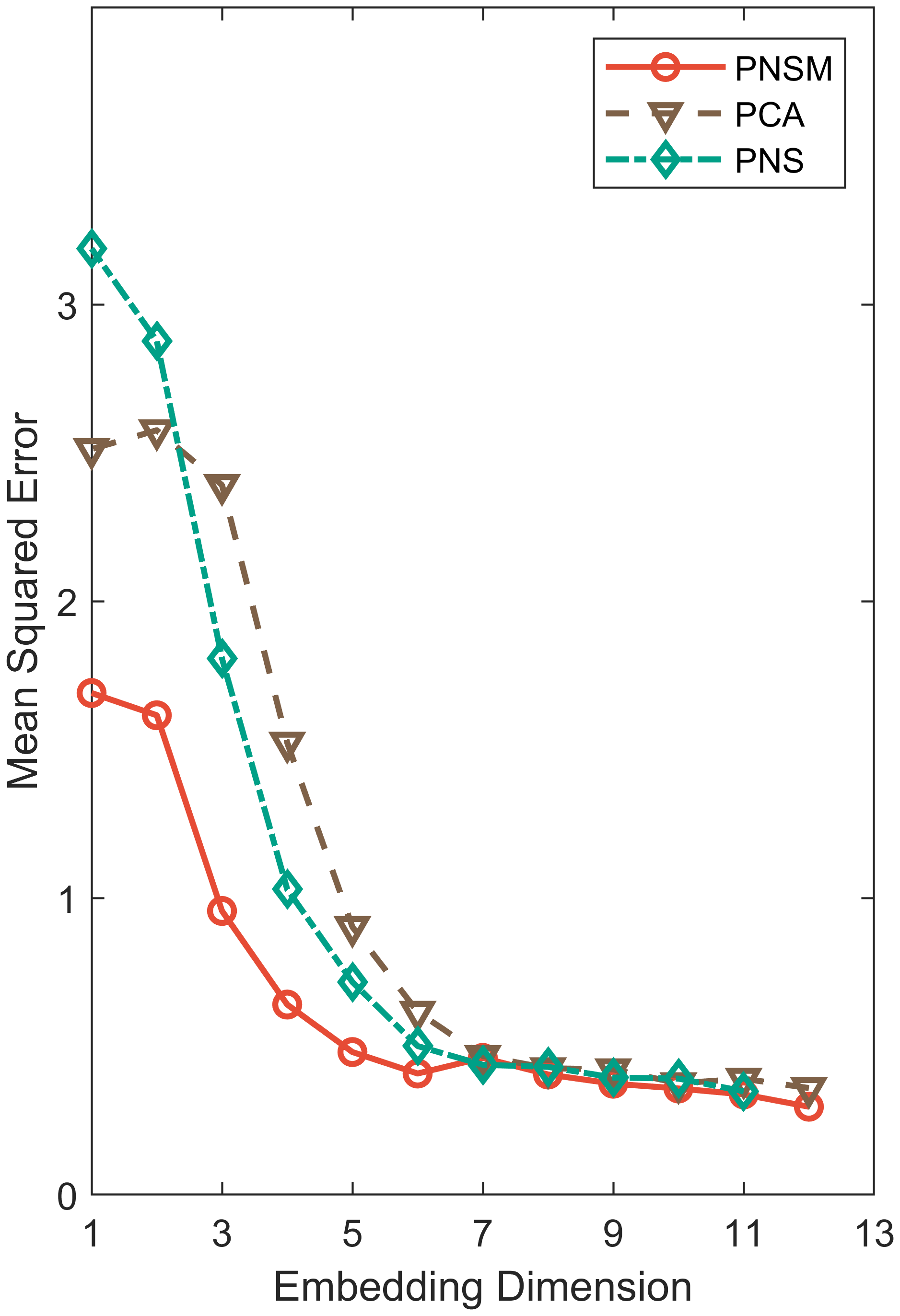
Figure 8: The average silhouette index (a), proportion of variation (b), and mean square error (c) for principal nested submanifolds (PNSM), principal component analysis (PCA), and principal nested spheres (PNS) at each projection step

Prior to dimensionality reduction and subsequent analysis, the data undergoes further processing. To ensure the accurate estimation of principal directions, we initially remove outliers. We calculate the pairwise Euclidean distance between sample points, construct a neighbourhood network with $r=6$, and eliminate points with fewer than 25 neighbours. This refinement process results in 6,528 samples remaining for further analysis. The distribution of these samples is summarized in the Appendix and illustrated through a two-dimensional t-distributed stochastic neighbour embedding in Figure 9(a). Compared to the original sample set (refer to Figure 1b in (Haber et al., 2017)), this process predominantly excludes most Enteroendocrine and Tuft cells, as they are positioned farther from the majority of cells and exhibit a broader spread. Although the clustering of cells appears distinct, there is potential for further enhancement.

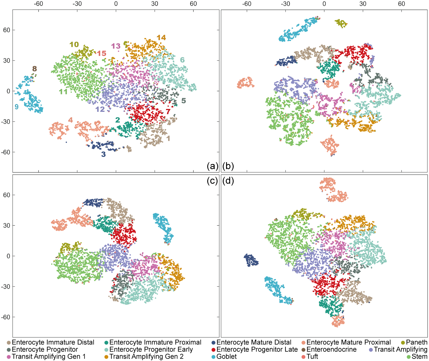
Figure 9: Scatter plots for the two-dimensional t-distributed stochastic neighbour embedding of (a) cleaned data set; (b) the principal nested submanifolds with $d=3$; (c) principal component analysis with $d=6$; (d) the principal nested spheres with $d=5$.

To enhance the clustering results, further analysis is conducted on the cleaned data set using our proposed method, principal component analysis, and principal nested spheres. In our method, we set the radius to $r=6$, and sequentially fit submanifolds with codimensions ranging from 1 to 12. For principal component analysis, we compute the covariance matrix of the samples and project the samples onto linear subspaces of dimensions 1 to 12. To apply principal nested spheres to this data set, we normalize each sample, use the unit vectors on $\mathcal{S}^{12}$ as inputs for the algorithm to fit nested spheres with dimensions 1 to 11, and then restore the norms of the output vectors to their original values. Eventually, we obtain projections of the samples in various dimensions using different methods for cluster analysis and method comparison.

In the dimension reduction process, we evaluate the performance using three metrics: the average silhouette index, the proportion of variation, and the mean square error at each projection step. The proportion of variation is computed in the conventional manner for principal component analysis and the linear embeddings of principal nested spheres. For principal nested submanifolds, however, it is estimated using the minimum sum of squared shortest paths on the nearest neighbor graph of the samples as an estimation for the geodesic distances. Figure 8 illustrates that the average silhouette index, whose value corresponds to our method initially increases, reaching a peak at $d=3$, and then starts to decline. This pattern suggests that the principal nested submanifolds improve clustering with the 15 provided labels. By comparison, the average silhouette indices for the other methods similarly rise and then fall; however, their peaks occur at higher dimensions, and their maximum values are lower than those of our method. This indicates that our approach more effectively captures low-dimensional structures and enhances clustering results.

Figures 8 and 8 display the proportion of variation in each subspace and the mean squared error associated with the fitting of the subspace, respectively. Our method produces an approximately linearly decreasing curve at higher dimensions, with a marked shift between dimensions 3 and 4 that results in a significant increase at lower dimensions. This pattern suggests that our method effectively removes variation from the data at each step, thereby facilitating the data decomposition. In contrast, the other two methods exhibit only minor changes at the initial dimensions but experience substantial alterations when the dimensionality is below 5. This behavior reflects their tendency to capture more information at lower dimensions. However, as Figure 8 illustrates, all three methods demonstrate gradually increasing mean squared errors, with our method consistently showing the lowest values. This advantage arises from our method is capable to more thoroughly evaluate and utilize nonlinear structures, allowing for a more extensive decomposition of variation with reduced mean squared error. Consequently, our method more effectively describes RNA data in lower dimensions, thereby enhancing the efficacy of clustering.

Figure 9 visualizes the two-dimensional t-distributed stochastic neighbour embedding of the input data alongside the configurations with the highest average silhouette index from the three examined methods. The figure of the principal nested submanifolds reveals that the proposed method modifies the data distribution while maintaining inter-group relationships. For instance, the Paneth (group 10) stands out distinctly from the majority. Moreover, the boundaries between the Stem, Transit Amplifying, Transit Amplifying Gen 1, and Transit Amplifying Gen 2 (groups 11–14) are more sharply defined compared to the other methods, indicating superior performance. Furthermore, our method promotes the emergence of additional subclasses within the samples. Groups such as Enterocyte Mature Proximal, Enterocyte Progenitor, Enterocyte Progenitor Early, Stem, and Transit Amplifying Gen 2 (groups 4–6, 11, and 14) exhibit clearer subclass distinctions. While this feature increases the intra-group distance, thereby slightly diminishing the silhouette index performance, it provides a novel insight into the clustering of these single-cell RNA data that is not captured by the alternative methods. Additional scatter plots of the embeddings under different dimensions of these three methods are available in the Appendix.

6 Discussion

In this paper, we explore the problem of nonlinear dimension reduction and data decomposition by introducing the principal nested submanifolds. This method extends the traditional principal component analysis by fitting a sequence of submanifolds of decreasing dimensionality instead of linear subspaces. We show that the population principal submanifolds are smooth submanifolds of the ambient space. In addition, we include algorithms for fitting these submanifolds. Through several simulation studies and analysis of a real-world single-cell RNA sequencing data set, we have shown the efficiency and potential applicability of our method across various fields.

The principal nested submanifolds approach is inspired by the manifold fitting framework and employs local covariance information to define each principal nested submanifold as a level set of a smooth function. By properly constructing this function, the resulting level sets are naturally nested and can be characterized as low-dimensional manifolds of the ambient space under mild conditions. This approach addresses the model bias problem present in related works such as those of Jung et al. (2012) and Eltzner et al. (2018). Moreover, we introduce a procedure that efficiently approximates these submanifolds, offering improvements over the methods proposed by Donnell et al. (1994), Panaretos et al. (2014), and Yao et al. (2026).

In numerical studies, the principal nested submanifolds method stands out. The simulation section uses specially designed cases in Euclidean spaces, spheres, and tori to illustrate the advantages of our method over traditional principal component analysis, principal nested spheres, and torus principal component analysis. It captures more complex structures and significantly reduces model bias. In addition, when analyzing single-cell RNA sequencing data, the principal nested submanifolds method outperforms other approaches by effectively removing less significant information and revealing distinct patterns in the data. This advances our understanding of nonlinear space decomposition and provides a fundamental framework for future advances in nonlinear embedding and complex data analysis. With potential applications in fields as diverse as neuroscience and machine learning, our framework provides a more intuitive understanding of data structures and their dynamics.

However, several challenges remain to be addressed. First, controlling the dimensionality of the fitted submanifolds requires numerous singular value decomposition steps. Although parallel computing with graphical processing units significantly reduces the computational time, more efficient computational strategies are needed. Furthermore, unlike principal component analysis and principal nested spheres, which yield Euclidean-like embeddings where each coordinate can be interpreted as the residual between two adjacent subspaces, this interpretation is less straightforward in nonlinear cases. Issues such as deciding the sign of the residual and distinguishing between two residual curves of the same length and sign require further mathematical exploration.

Appendices

A.1 Proof omitted from the main text

Proof.

Let $p$ be a fixed point on $\mathcal{M}_{r,d}$, and $z\in\mathcal{B}(p,\eta)$ be another point of interest. For the sake of simplicity, we denote the collection of principal directions at $z$ as $V_{z}=(v_{r,z,1},\dots,v_{r,z,D-d})$, the summation of projection matrices as

$$\Psi_{z}=V_{z}V_{z}^{\top}=\sum_{k=1}^{D-d}\Pi_{r,z,k},$$

and the summation of bias vectors as the bias function

$$b(z)=\Psi_{z}(z-\mu_{z})=\sum_{k=1}^{D-d}b_{r,k}(z),$$

for all $z$ of interest. To prove Theorem 1, we need the following lemmas.

Lemma A.1.

With Conditions 1–3 and the set up of Theorem 1, the Jacobian matrix of $b(z)$ satisfies

$$\|\textnormal{J}_{b}(z)-\Psi_{z}\|\leq(D-d)(r\ell_{3}+\ell_{5}),$$

for all $z\in\mathcal{B}(p,\eta)$.

Proof.

Let $u$ be a unit vector in $\mathbb{R}^{D}$, the directional derivative of $b(z)$ along $u$ is

$$\partial_{u}b(z)=(\partial_{u}\Psi_{z})(z-\mu_{z})+\Psi_{z}u-\Psi_{z}(\partial_{u}\mu_{z}),$$

which leads to

$$\|\partial_{u}b(z)-\Psi_{z}u\|\leq\|(\partial_{u}\Psi_{z})(z-\mu_{z})\|+\|\Psi_{z}(\partial_{u}\mu_{z})\|.$$

The first term can be upper bounded as

$$\|(\partial_{u}\Psi_{z})(z-\mu_{z})\| \leq\|z-\mu_{z}\|\left\|\sum_{k=1}^{D-d}\partial_{u}\Pi_{r,z,k}\right\|$$

$$\leq\sum_{k=1}^{D-d}\|z-\mu_{z}\|\left\|\partial_{u}\Pi_{r,z,k}\right\|$$

$$\leq(D-d)r\ell_{3},$$

where the last inequality is due to the fact that $\mu_{z}\in\mathcal{B}(z,r)$. For the second term, there is

$$\|\Psi_{z}(\partial_{u}\mu_{z})\| =\left\|\sum_{k=1}^{D-d}v_{r,z,k}v_{r,z,k}^{\top}\textnormal{J}_{\mu}(z)u\right\|$$

$$\leq\sum_{k=1}^{D-d}\|v_{r,z,k}\|\left\|v_{r,z,k}^{\top}\textnormal{J}_{\mu}(z)\right\|\|u\|$$

$$<(D-d)\ell_{5},$$

where $\textnormal{J}_{\mu}(z)$ denotes the Jacobian matrix of $\mu_{z}$ at point $z$. Then, by definition

$$\|\textnormal{J}_{b}(z)-\Psi_{z}\| =\sup_{u\in\mathbb{R}^{D}}\frac{\|\textnormal{J}_{b}(z)u-\Psi_{z}u\|}{\|u\|}$$

$$<(D-d)(r\ell_{3}+\ell_{5}),$$

for all $z\in\mathcal{B}(p,\eta)$, which completes the proof. ∎

Lemma A.2.

With Conditions 1–3 and the set up of Theorem 1, for two unit vectors $u,u^{\prime}\in\mathbb{R}^{D}$,

$$\|\partial_{u}\partial_{u^{\prime}}b(z)\|\leq(D-d)\bigl{\{}r\ell_{4}+\ell_{2}+2\ell_{3}(1+\ell_{1})\bigl{\}}$$

for all $z\in\mathcal{B}(p,\eta)$.

Proof.

By definition and the triangle inequality, an upper bound of $\|\partial_{u}\partial_{u^{\prime}}b(z)\|$ is given by

$$\|\partial_{u}\partial_{u^{\prime}}b(z)\|\leq \|(\partial_{u}\partial_{u^{\prime}}\Psi_{z})(z-\mu_{z})\|+\|\Psi_{z}\partial_{u}\partial_{u^{\prime}}(z-\mu_{z})\|$$

$$+\|(\partial_{u}\Psi_{z})\partial_{u^{\prime}}(z-\mu_{z})\|+\|(\partial_{u^{\prime}}\Psi_{z})\partial_{u}(z-\mu_{z})\|.$$

For the first term,

$$\|(\partial_{u}\partial_{u^{\prime}}\Psi_{z})(z-\mu_{z})\| =\left\|\sum_{k=1}^{D-d}\partial_{u}\partial_{u^{\prime}}\Pi_{r,z,k}\right\|\|z-\mu_{z}\|$$

$$\leq\sum_{k=1}^{D-d}r\left\|\partial_{u}\partial_{u^{\prime}}\Pi_{r,z,k}\right\|$$

$$\leq(D-d)r\ell_{4}.$$

For the second term,

$$\|\Psi_{z}\partial_{u}\partial_{u^{\prime}}(z-\mu_{z})\| =\left\|\sum_{k=1}^{D-d}v_{r,z,k}v_{r,z,k}^{\top}(\partial_{u}\partial_{u^{\prime}}\mu_{z})\right\|$$

$$\leq\sum_{k=1}^{D-d}\left\|v_{r,z,k}^{\top}(\partial_{u}\partial_{u^{\prime}}\mu_{z})\right\|$$

$$\leq(D-d)\ell_{2}.$$

For the last two terms,

$$\|(\partial_{u}\Psi_{z})\partial_{u^{\prime}}(z-\mu_{z})\| =\|(\partial_{u}\Psi_{z})(u^{\prime}-\partial_{u^{\prime}}\mu_{z})\|$$

$$\leq\|\partial_{u}\Psi_{z}\|\bigl{(}1+\|\partial_{u^{\prime}}\mu_{z}\|\bigl{)}$$

$$\leq(D-d)\ell_{3}(1+\ell_{1}).$$

Hence,

$$\|\partial_{u}\partial_{u^{\prime}}b(z)\|\leq(D-d)\bigl{\{}r\ell_{4}+\ell_{2}+2\ell_{3}(1+\ell_{1})\bigl{\}},$$

for all $z\in\mathcal{B}(p,\eta)$. ∎

Lemma A.3 (Constant-Rank Level Set Theorem (Theorem 5.12 of (Lee, 2012))).

Let $\mathcal{S}_{1}$ and $\mathcal{S}_{2}$ be smooth manifolds, and let $\Phi:\,\mathcal{S}_{1}\to\mathcal{S}_{2}$ be a smooth map with constant rank $k$. Each level set of $\Phi$ is a properly embedded submanifold of codimension $k$ in $\mathcal{S}_{1}$.

Lemma A.4 (Implicit Function Theorem (Theorem C.40 of (Lee, 2012))).

Let $\mathcal{U}\subseteq\mathbb{R}^{d_{1}}\times\mathbb{R}^{d_{2}}$ be an open subset, and let $(s,t)=(s_{1},\dots,s_{d_{1}},t_{1},\dots,t_{d_{2}})$ denote the standard coordinates on $\mathcal{U}$. Suppose $\Phi:\,\mathcal{U}\to\mathbb{R}^{d_{2}}$ is a smooth function, $(s^{*},t^{*})\in\mathcal{U}$, and $\Phi(s^{*},t^{*})=0$. If the $d_{2}\times d_{2}$ matrix

$$\left(\frac{\partial\Phi_{i}}{\partial t_{j}}(s^{*},t^{*})\right)$$

is nonsingular, then there exist neighbourhoods $\mathcal{V}_{1}\subseteq\mathbb{R}^{d_{1}}$ of $s^{*}$ and $\mathcal{V}_{2}\subseteq\mathbb{R}^{d_{2}}$ of $t^{*}$ and a smooth function $\varphi:\,\mathcal{V}_{1}\to\mathcal{V}_{2}$ such that $\Phi^{-1}(0)\cap\mathcal{V}_{1}\times\mathcal{V}_{2}$ is the graph of $\varphi$, that is, $\Phi(s,t)=0$ for $(x,y)\in\mathcal{V}_{1}\times\mathcal{V}_{2}$ if and only if $t=\varphi(s)$.

After introducing these preparative lemmas, let us consider an ancillary function $h(z):\mathcal{B}(p,\eta)\to\mathbb{R}^{D-d}$ given by

$$h(z)=V_{p}^{\top}b(z)=V_{p}^{\top}\Psi_{z}(z-\mu_{z}).$$

We first prove for all $z\in\mathcal{B}(p,\eta)$, $b(z)=0$ if and only if $h(z)=0$.

Since it is obvious that

$$\{z:b(z)=0\}\subset\{z:h(z)=0\},$$

it is sufficient to show the other direction.
Assume there is a point $q\in\mathcal{B}(p,\eta)$ such that $h(q)=0$ but $b(q)\neq 0$. Then, there is

$$\|\Psi_{p}-\Psi_{q}\| =\sup_{u\in\mathbb{R}^{D}}\frac{\|(\Psi_{p}-\Psi_{q})u\|}{\|u\|}$$

$$\geq\frac{\|(\Psi_{p}-\Psi_{q})b(q)\|}{\|b(q)\|}$$

$$=\frac{\|V_{p}V_{p}^{\top}b(q)-\Psi_{q}b(q)\|}{\|b(q)\|}$$

$$=\frac{\|V_{p}h(q)-b(q)\|}{\|b(q)\|}$$

$$=\frac{\|0-b(q)\|}{\|b(q)\|}$$

$$=1,$$

which, together with (2) and the fact that $\|p-q\|<\eta$, leads to the result that

$$\sup_{z\in\mathcal{B}(p,\eta)}\|\partial_{u}\Psi_{z}\| \geq\|\Psi_{p}-\Psi_{q}\|/\|p-q\|$$

$$\geq\eta^{-1}$$

$$\geq\frac{(D-d)\bigl{\{}r\ell_{4}+\ell_{2}+2\ell_{3}(1+\ell_{1})\bigl{\}}}{1-(D-d)(r\ell_{3}+\ell_{5})}$$

$$>(D-d)\bigl{\{}r\ell_{4}+\ell_{2}+2\ell_{3}(1+\ell_{1})\bigl{\}}$$

$$>2(D-d)\ell_{3}$$

is contradictory to the assumption that

$$\sup_{z\in\mathcal{B}(p,\eta)}\|\partial_{u}\Psi_{z}\| \leq\sum_{k=1}^{D-d}\sup_{z\in\mathcal{B}(p,\eta)}\left\|\partial_{u}\Pi_{r,z,k}\right\|$$

$$\leq(D-d)\ell_{3}.$$

Hence, $b(z)=0$ if and only if $h(z)=0$ for $z\in\mathcal{B}(p,\eta)$.

Next, we investigate the Jacobian matrix of $h(z)$.

For any $z\in\mathcal{B}(p,\eta)$,

$$\textnormal{J}_{h}(z) =V_{p}^{\top}\textnormal{J}_{b}(z)$$

$$=V_{p}^{\top}\{\textnormal{J}_{b}(z)-\textnormal{J}_{b}(p)\}+V_{p}^{\top}\{\textnormal{J}_{b}(p)-\Psi_{p}\}+V_{p}^{\top}\Psi_{p}.$$

Since $V_{p}^{\top}\Psi_{p}=V_{p}^{\top}$, there is

$$\|\textnormal{J}_{h}(z)-V_{p}^{\top}\| \leq\|V_{p}^{\top}\{\textnormal{J}_{b}(z)-\textnormal{J}_{b}(p)\}\|+\|V_{p}^{\top}\{\textnormal{J}_{b}(p)-\Psi_{p}\}\|$$

$$\leq\|\textnormal{J}_{b}(z)-\textnormal{J}_{b}(p)\|+\|\textnormal{J}_{b}(p)-\Psi_{p}\|$$

$$\leq\|z-p\|\sup_{\begin{subarray}{c}z^{\prime}\in\mathcal{B}(p,\eta)\\ \|u\|=\|u^{\prime}\|=1\end{subarray}}\|\partial_{u}\partial_{u^{\prime}}b(z^{\prime})\|+\sup_{z^{\prime}\in\mathcal{B}(p,\eta)}\|\textnormal{J}_{b}(z^{\prime})-\Psi_{z^{\prime}}\|$$

$$<\eta(D-d)\bigl{\{}r\ell_{4}+\ell_{2}+2\ell_{3}(1+\ell_{1})\bigl{\}}+(D-d)(r\ell_{3}+\ell_{5})$$

$$<1,$$

which suggests that the maximal difference between the singular values of $\textnormal{J}_{h}(z)$ and $V_{p}^{\top}$ is less than $1$. Because the column of $V_{p}$ are orthogonal unit vectors and thus its singular values are all $1$, there is ${\operatorname{rank}}\bigl{(}\textnormal{J}_{h}(z)\bigl{)}=D-d$. According to the Constant-Rank Level Set Theorem, the level set

$$\{z\in\mathcal{B}(p,\eta):b(z)=0\}=\{z\in\mathcal{B}(p,\eta):h(z)=0\}=\mathcal{M}_{r,d}\cap\mathcal{B}(p,\eta)$$

is a $d$-dimensional embedded submanifold of $\mathcal{B}(p,\eta)\subseteq\mathbb{R}^{D}$. Since this result holds for every $p\in\mathcal{M}_{r,d}$, we can state that $\mathcal{M}_{r,d}$ is topologically a $d$-dimensional submanifold of $\mathbb{R}^{D}$.

Moreover, if $\mathcal{M}_{r,d}$ is a connected set, ${\operatorname{reach}}(\mathcal{M}_{r,d})$ can be bounded below.

Recall that, the reach of ${\operatorname{reach}}(\mathcal{M}_{r,d})$ can be given by

$${\operatorname{reach}}(\mathcal{M}_{r,d})=\inf_{z,z^{\prime}\in\mathcal{M}_{r,d}}\frac{\|z-z^{\prime}\|^{2}}{2\operatorname*{d}(z^{\prime},T_{z}\mathcal{M}_{r,d})}.$$

We first consider the case where the two points are close, that is, for $p\in\mathcal{M}_{r,d}$, we consider another point $q\in\mathcal{M}_{r,d}$ with $p\neq q$ and $\|p-q\|\leq\eta$. Since we have already shown that $\mathcal{B}(p,\eta)\cap\mathcal{M}_{r,d}$ homeomorphic to a $d$-dimensional Euclidean space, let the collection of the unit basis vectors of $T_{p}\mathcal{M}_{r,d}$ be $W_{p}\in\mathbb{R}^{D\times d}$, and $W_{p}^{\perp}$ be its complement in $\mathbb{R}^{D}$. Without loss of generality, let the column span space of $W_{p}$ be corresponding to the first $d$ coordinates, the column span space of $W_{p}^{\perp}$ be corresponding to the last $D-d$ coordinates, and for each $z\in\mathcal{B}(p,\eta)$ let

$$s_{z}=W_{p}^{\top}(z-p)\in\mathbb{R}^{d},\quad t_{z}=(W_{p}^{\perp})^{\top}(z-p)\in\mathbb{R}^{D-d},$$ (A.1)

denote the subset of coordinates. Since $\mathcal{M}_{r,d}$ is locally give by the root set of $h(z)$, there is

$$\textnormal{J}_{h}(p)W_{p}=0.$$

According to the Implicit Function Theorem and the results above, there exists a function $g(\cdot)$ such that, for $z\in\mathcal{B}(p,\eta)$, $h(z)=h(s_{z},t_{z})=0$ if and only if $t_{z}=g(s_{z})$. Then, by calculating the derivate of $h(s,g(s))=0$, there is

$$0 =\textnormal{D}_{s}h(s,g(s))+\textnormal{D}_{t}h(s,g(s))\textnormal{D}_{s}g(s)$$

$$=\textnormal{J}_{h}\bigl{(}s,g(s)\bigl{)}W_{p}+\textnormal{J}_{h}\bigl{(}s,g(s)\bigl{)}W_{p}^{\perp}\textnormal{J}_{g}(s),$$

which leads to the result that the Jacobian of $g(s)$ can be expressed as

$$\textnormal{J}_{g}(s)=-\left\{\textnormal{J}_{h}\bigl{(}s,g(s)\bigl{)}W_{p}^{\perp}\right\}^{-1}\textnormal{J}_{h}\bigl{(}s,g(s)\bigl{)}W_{p},$$

and hence,

$$\|\textnormal{J}_{g}(s)\| =\|\left\{\textnormal{J}_{h}\bigl{(}s,g(s)\bigl{)}W_{p}^{\perp}\right\}^{-1}\textnormal{J}_{h}\bigl{(}s,g(s)\bigl{)}W_{p}\|$$

$$\leq\|\left\{\textnormal{J}_{h}\bigl{(}s,g(s)\bigl{)}W_{p}^{\perp}\right\}^{-1}\|\|\bigl{\{}\textnormal{J}_{h}\bigl{(}s,g(s)\bigl{)}-\textnormal{J}_{h}(p)\bigl{\}}W_{p}\|$$

$$\leq\left\{\lambda_{D-d}\Bigl{(}\textnormal{J}_{h}\bigl{(}s,g(s)\bigl{)}W_{p}^{\perp}\Bigl{)}\right\}^{-1}\|V_{p}^{\top}\|\|\bigl{\{}\textnormal{J}_{b}\bigl{(}s,g(s)\bigl{)}-\textnormal{J}_{b}(p)\bigl{\}}\|\|W_{p}\|,$$

where $\lambda_{D-d}(A)$ denotes the $(D-d)$th largest singular of matrix $A$. Since

$$\lambda_{D-d}\Bigl{(}\textnormal{J}_{h}\bigl{(}s,g(s)\bigl{)}W_{p}^{\perp}\Bigl{)} \geq\lambda_{D-d}\Bigl{(}V^{\top}_{p}\textnormal{J}_{b}\bigl{(}s,g(s)\bigl{)}\Bigl{)}\lambda_{\min}(W_{p}^{\perp})$$

$$\geq\lambda_{\min}(V^{\top}_{p})\lambda_{D-d}\Bigl{(}\textnormal{J}_{b}\bigl{(}s,g(s)\bigl{)}\Bigl{)}\lambda_{\min}(W_{p}^{\perp})$$

$$\geq 1-(D-d)(r\ell_{3}+\ell_{5}),$$

the norm of $\textnormal{J}_{g}(s)$ is further bounded as

$$\|\textnormal{J}_{g}(s)\| \leq\left\{\sigma_{D-d}\bigl{(}J_{b}\bigl{(}s,g(s)\bigl{)}\right\}^{-1}\|\textnormal{J}_{b}\bigl{(}s,g(s)\bigl{)}-\textnormal{J}_{b}(p)\|$$

$$\leq\|\bigl{(}s,g(s)\bigl{)}-p\|\frac{(D-d)\bigl{\{}r\ell_{4}+\ell_{2}+2\ell_{3}(1+\ell_{1})\bigl{\}}}{1-(D-d)(r\ell_{3}+\ell_{5})}.$$

Therefore, for any $p,q\in\mathcal{M}_{r,d}$, let $s_{p}$ and $s_{q}$ be defined as in (A.1), there is

$$\frac{\|p-q\|^{2}}{2\operatorname*{d}(q,T_{p}\mathcal{M}_{r,d})} =\frac{\|p-q\|^{2}}{2\|g(s_{p})-g(s_{q})\|}$$ (A.2)

$$\geq\frac{\|p-q\|^{2}}{2\|s_{p}-s_{q}\|\|\bigl{(}s_{q},g(s_{q})\bigl{)}-p\|}\frac{1-(D-d)(r\ell_{3}+\ell_{5})}{(D-d)\bigl{\{}r\ell_{4}+\ell_{2}+2\ell_{3}(1+\ell_{1})\bigl{\}}}$$

$$>\frac{\|p-q\|^{2}\eta}{2\|p-q\|\|\bigl{(}s_{q},g(s_{q})\bigl{)}-p\|}$$

$$\geq\frac{\eta}{2}.$$

Moreover, since $\operatorname*{d}(q,T_{p}\mathcal{M}_{r,d})\leq\|p-q\|$, for $p,q\in\mathcal{M}_{r,d}$ with $\|p-q\|>\eta$ there is

$$\frac{\|p-q\|^{2}}{2\operatorname*{d}(q,T_{p}\mathcal{M}_{r,d})}\geq\frac{\|p-q\|}{2}\geq\frac{\eta}{2}.$$ (A.3)

Combining the result in (A.2) and (A.3), for any $p\neq q\in\mathcal{M}_{r,d}$,

$$\frac{\|p-q\|^{2}}{2\operatorname*{d}(q,T_{p}\mathcal{M}_{r,d})}\geq\frac{\eta}{2},$$

which suggests that $\mathcal{M}_{r,d}$ is a $\mathcal{C}^{1}$ manifold with ${\operatorname{reach}}(\mathcal{M}_{r,d})\geq\eta/2$. ∎

A.2 Cell counts for the single-cell RNA data set

Table 1: Number of cells in each group before and after cleaning

Group	Cell Type	Count (Original)	Count (Cleaned)
1	Enterocyte Immature Distal	512	508
2	Enterocyte Immature Proximal	297	297
3	Enterocyte Mature Distal	241	179
4	Enterocyte Mature Proximal	581	555
5	Enterocyte Progenitor	356	356
6	Enterocyte Progenitor Early	829	828
7	Enterocyte Progenito Late	404	404
8	Enteroendocrine	310	37
9	Goblet	510	396
10	Paneth	260	217
11	Stem	1267	1263
12	Transit Amplifying	665	665
13	Transit Amplifying Gen 1	408	408
14	Transit Amplifying Gen 2	410	394
15	Tuft	166	21
	Total	7216	6528

A.3 Additional figures of the real data study

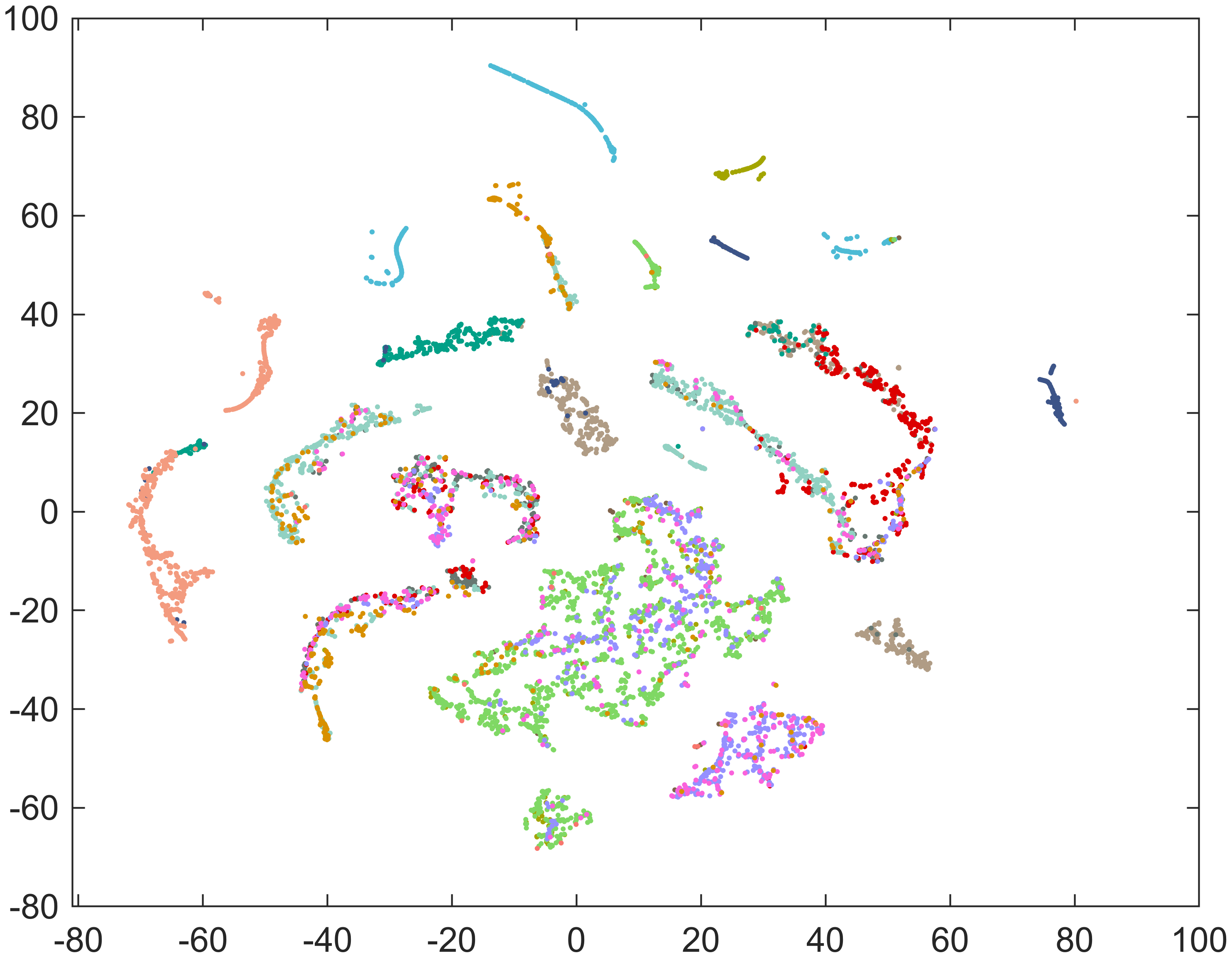
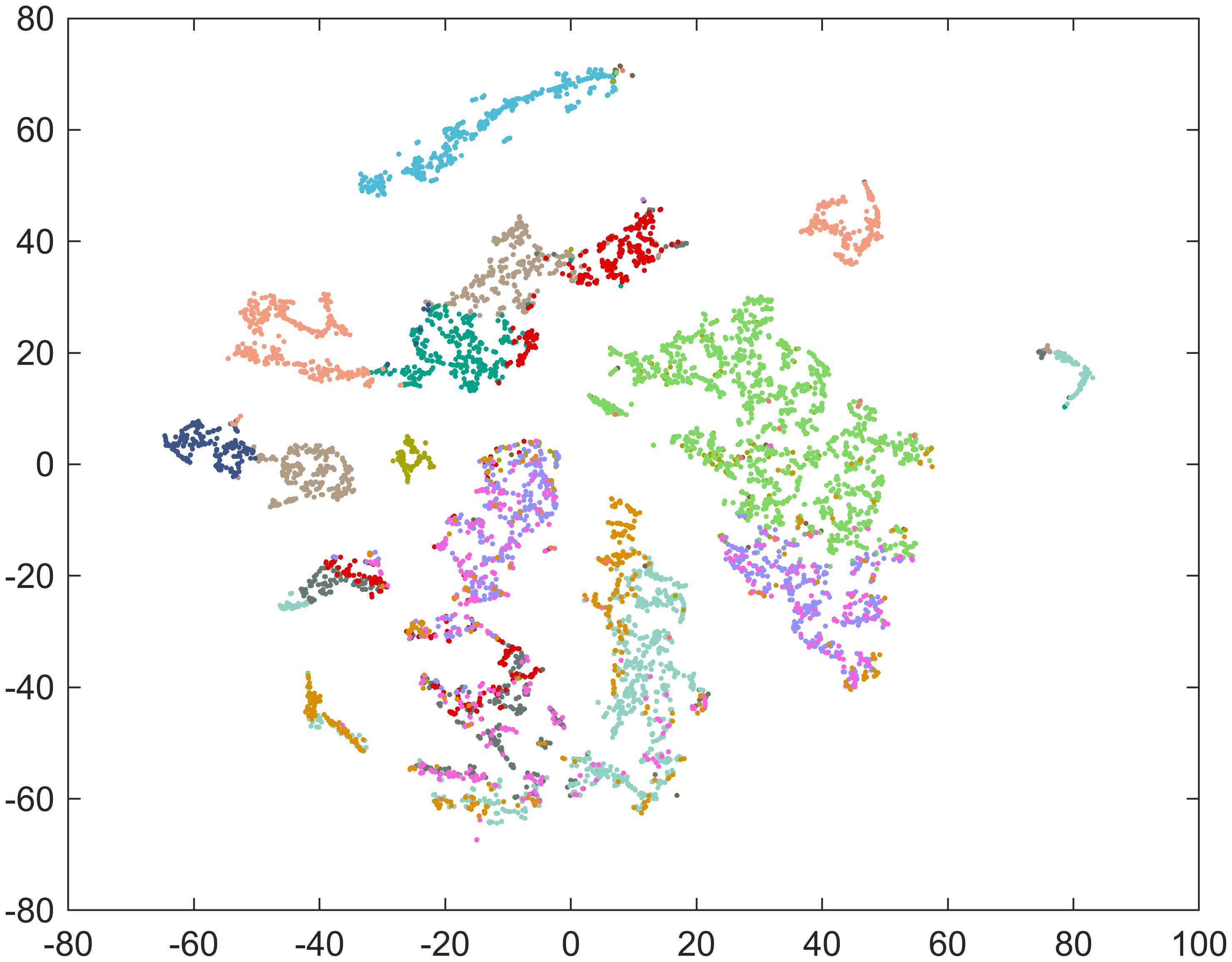
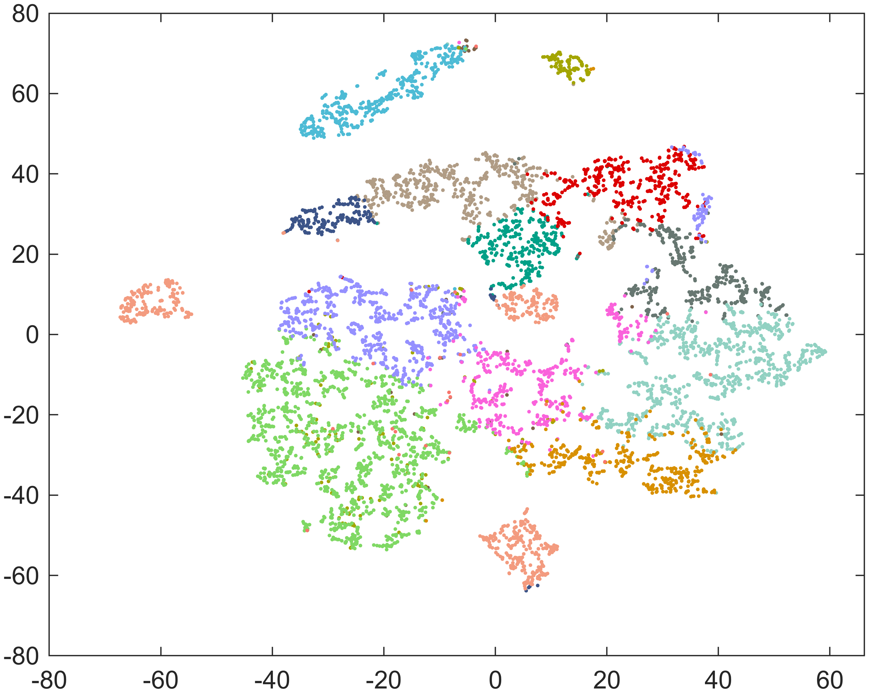
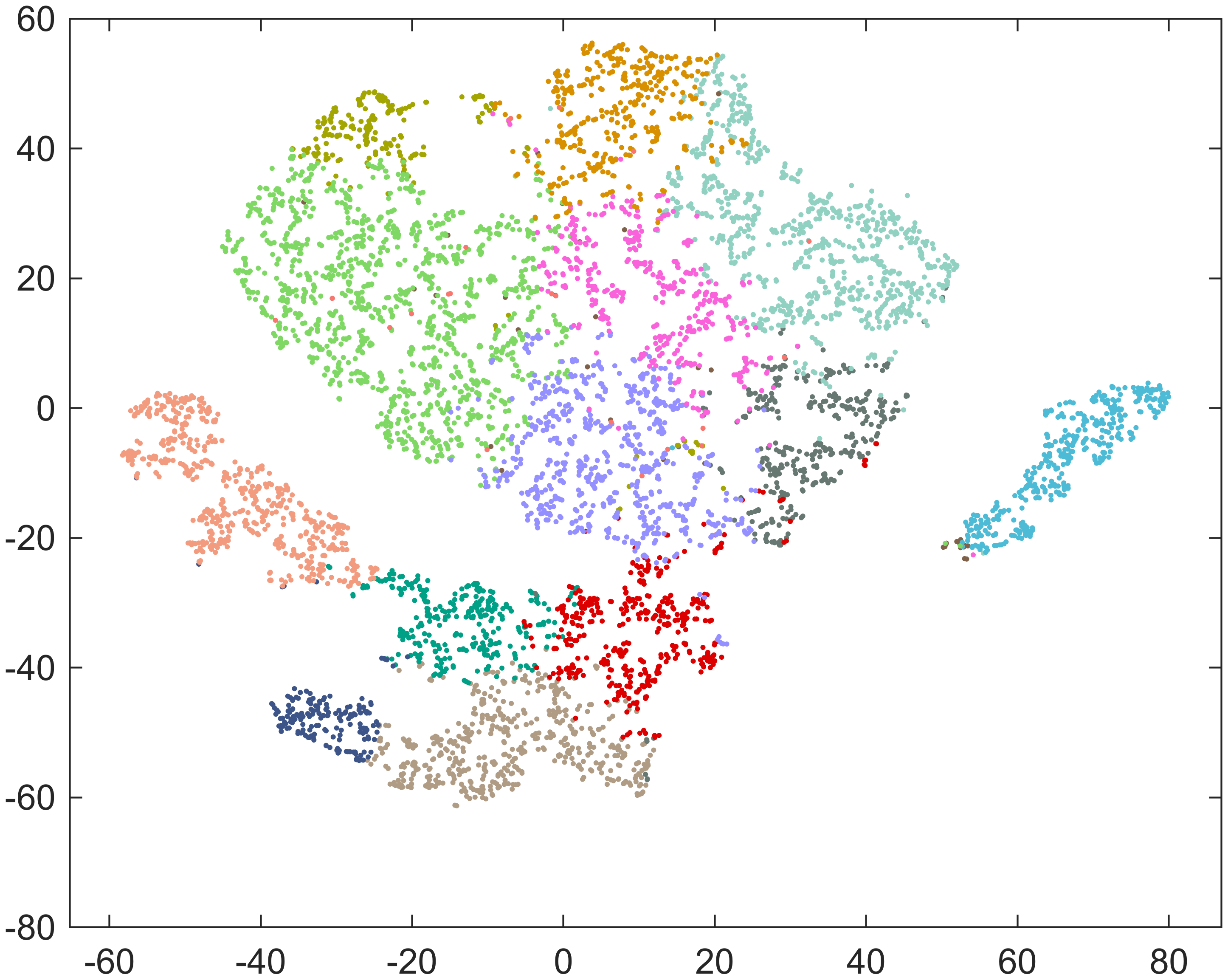
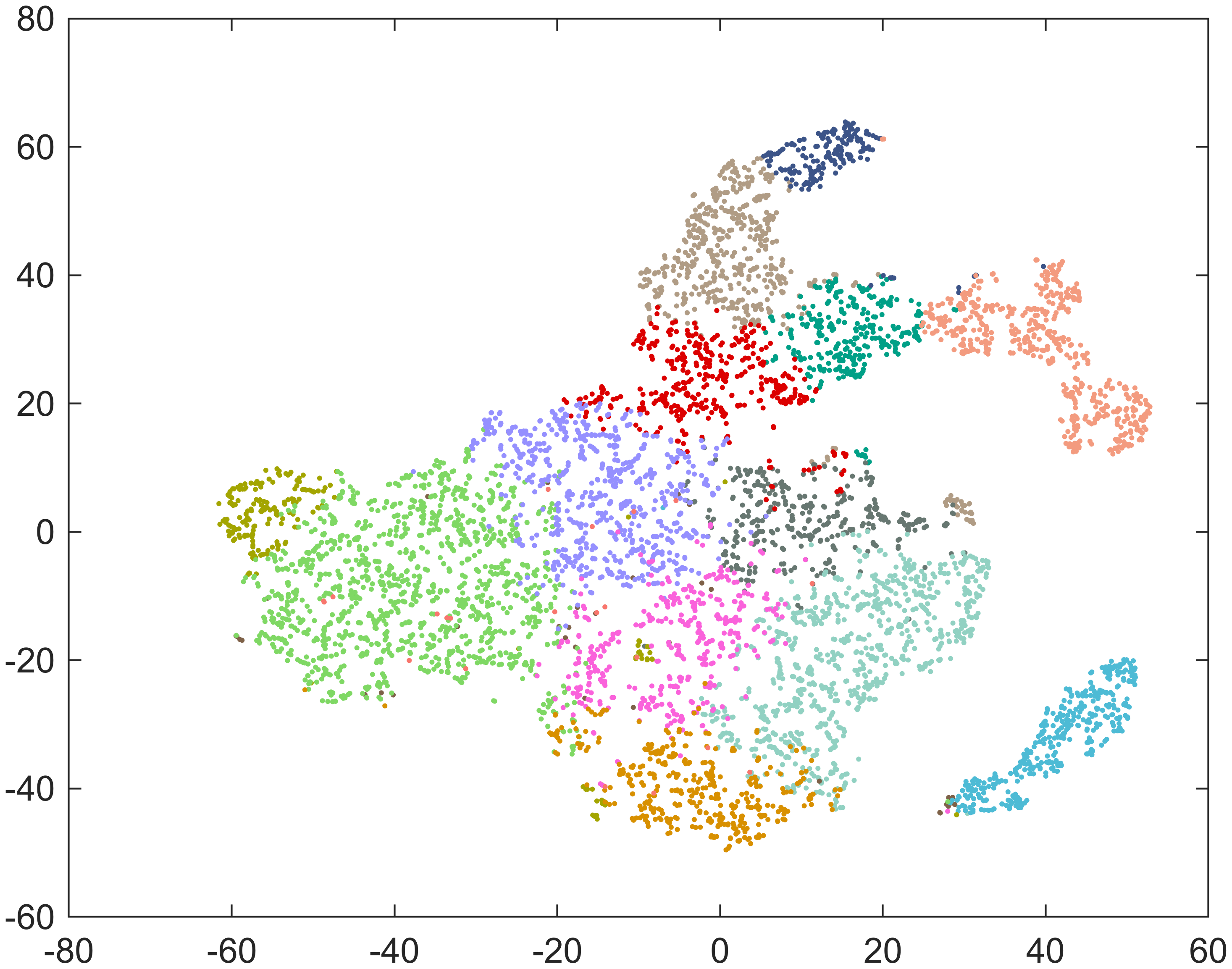
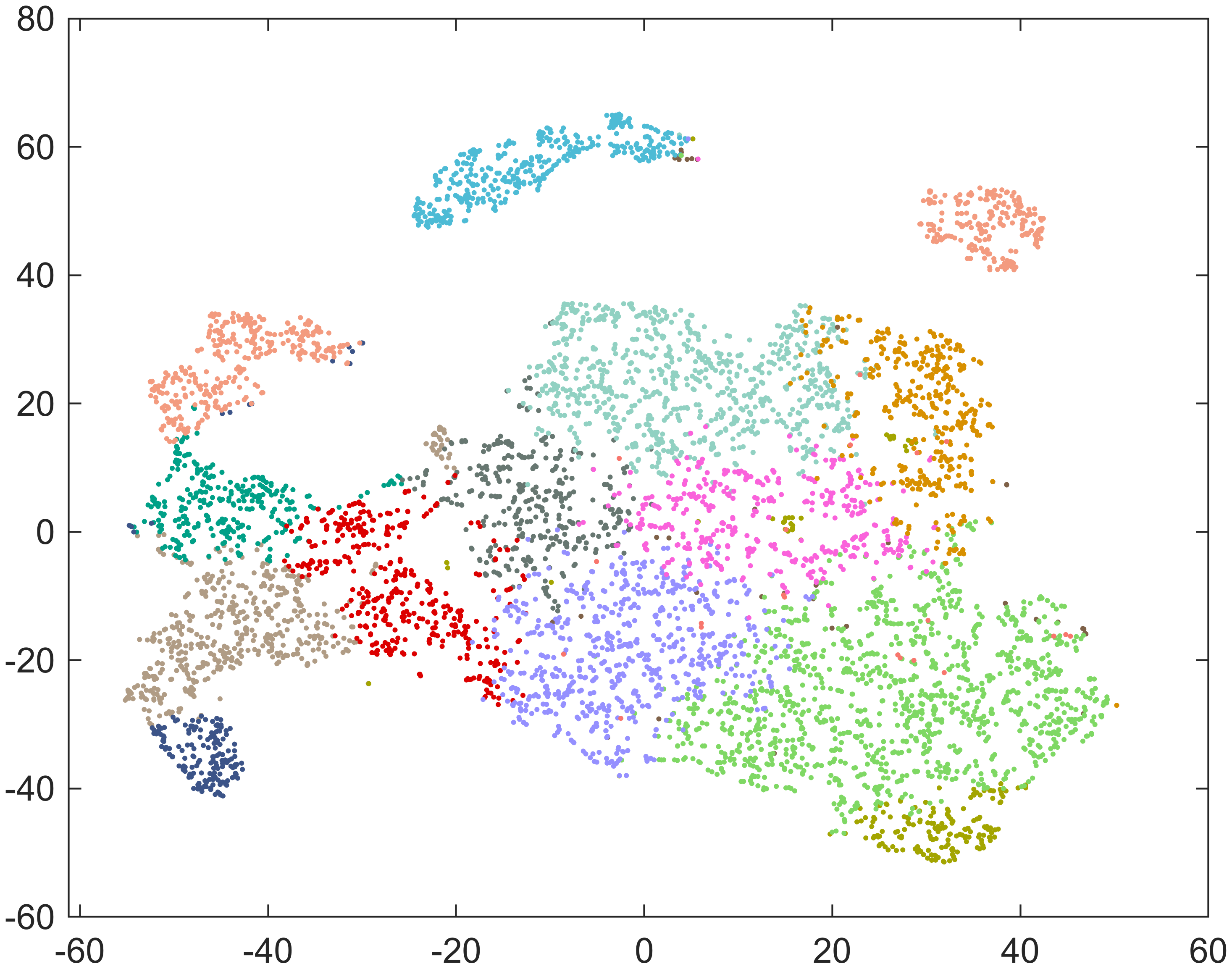
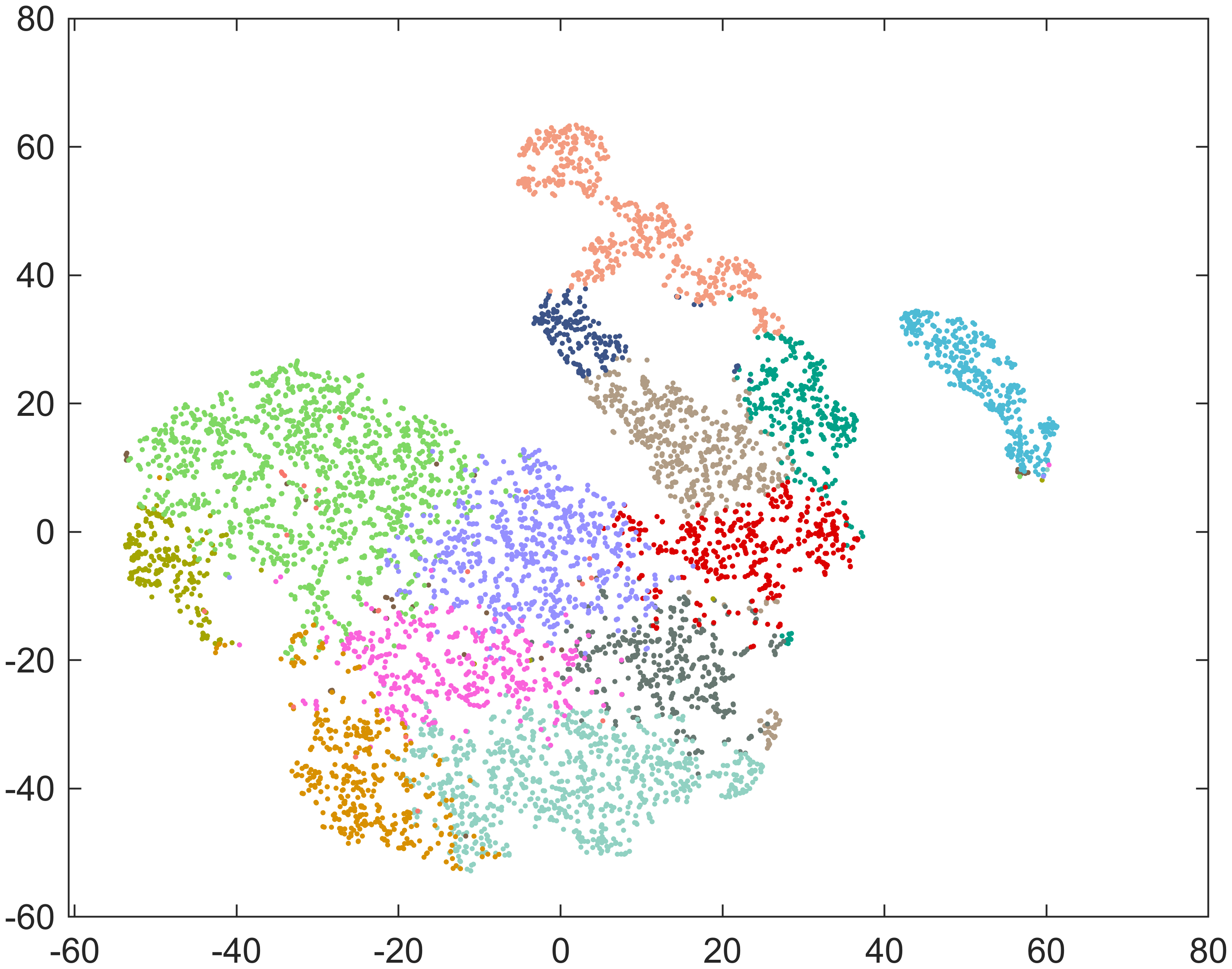
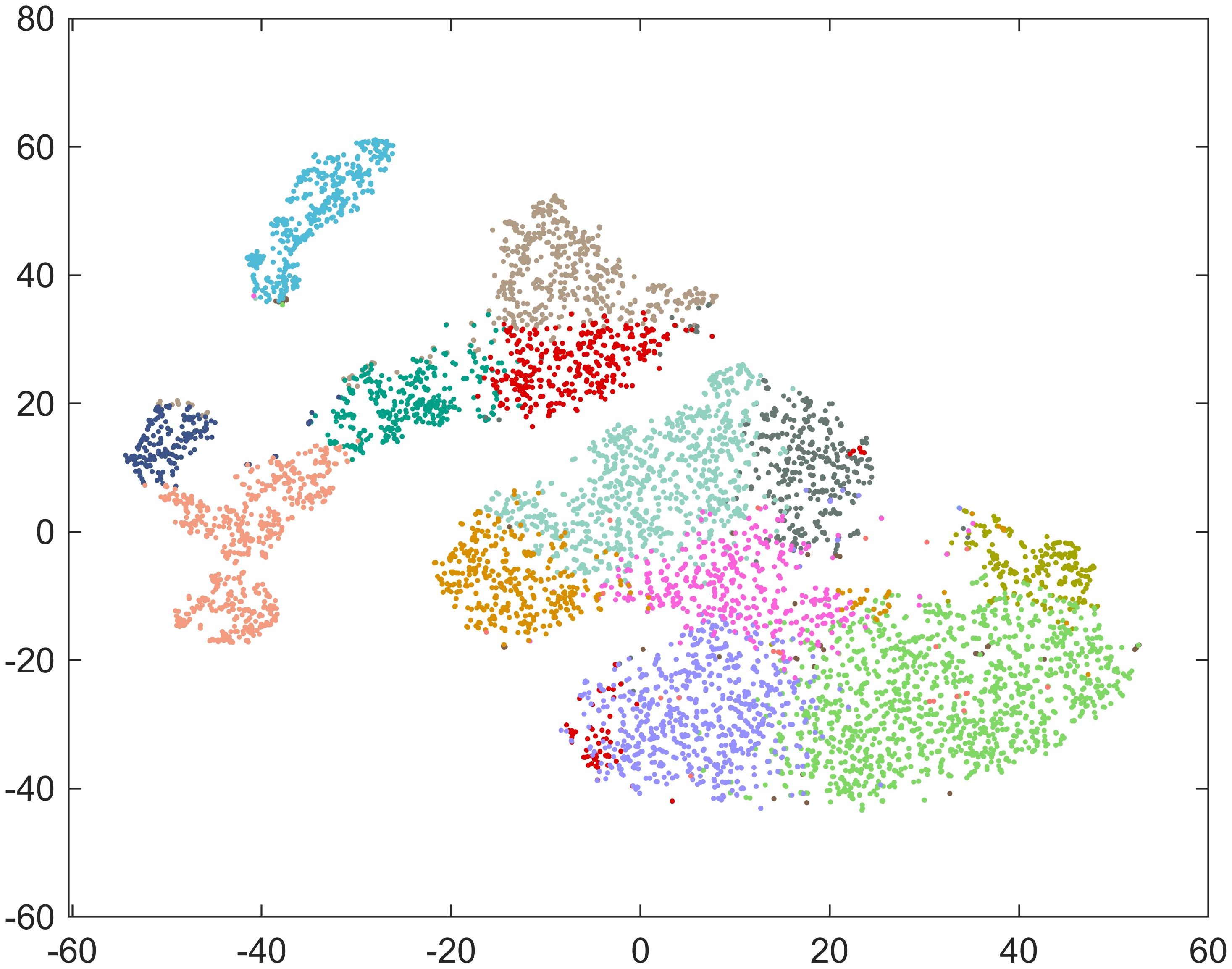
Figure A.1: Scatter plots for the two-dimensional t-distributed stochastic neighbour embedding of the result from the principal nested submanifolds with $d=1,\dots,12$ in (a)–(l).

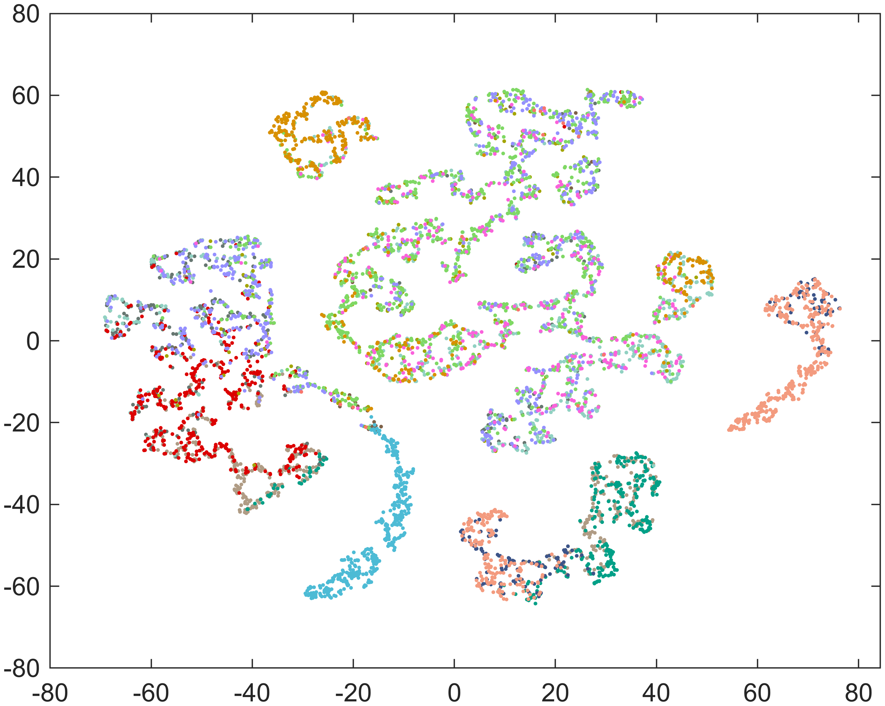
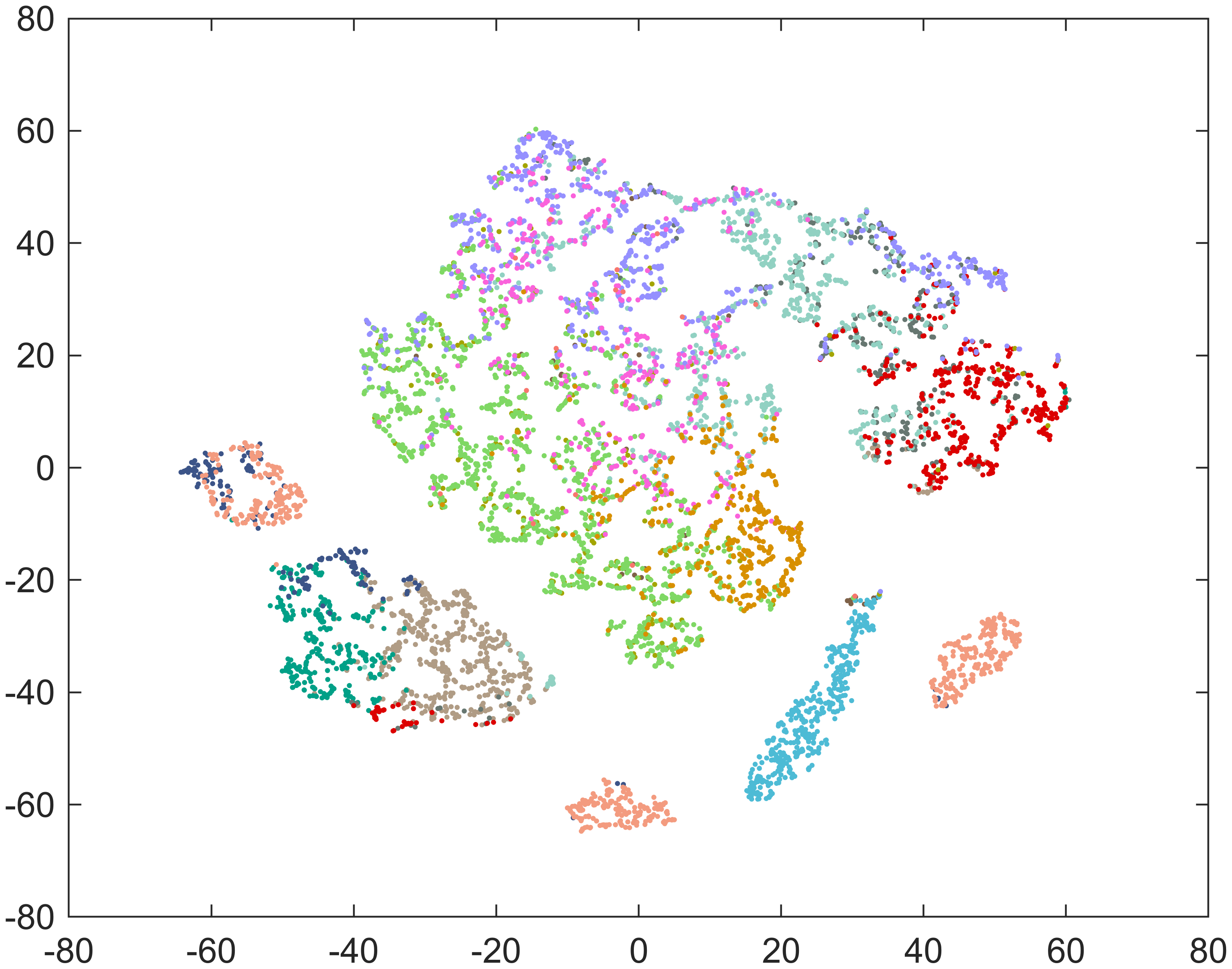
Figure A.2: Scatter plots for the two-dimensional t-distributed stochastic neighbour embedding of the result from the principal component analysis with $d=1,\dots,12$ in (a)–(l).

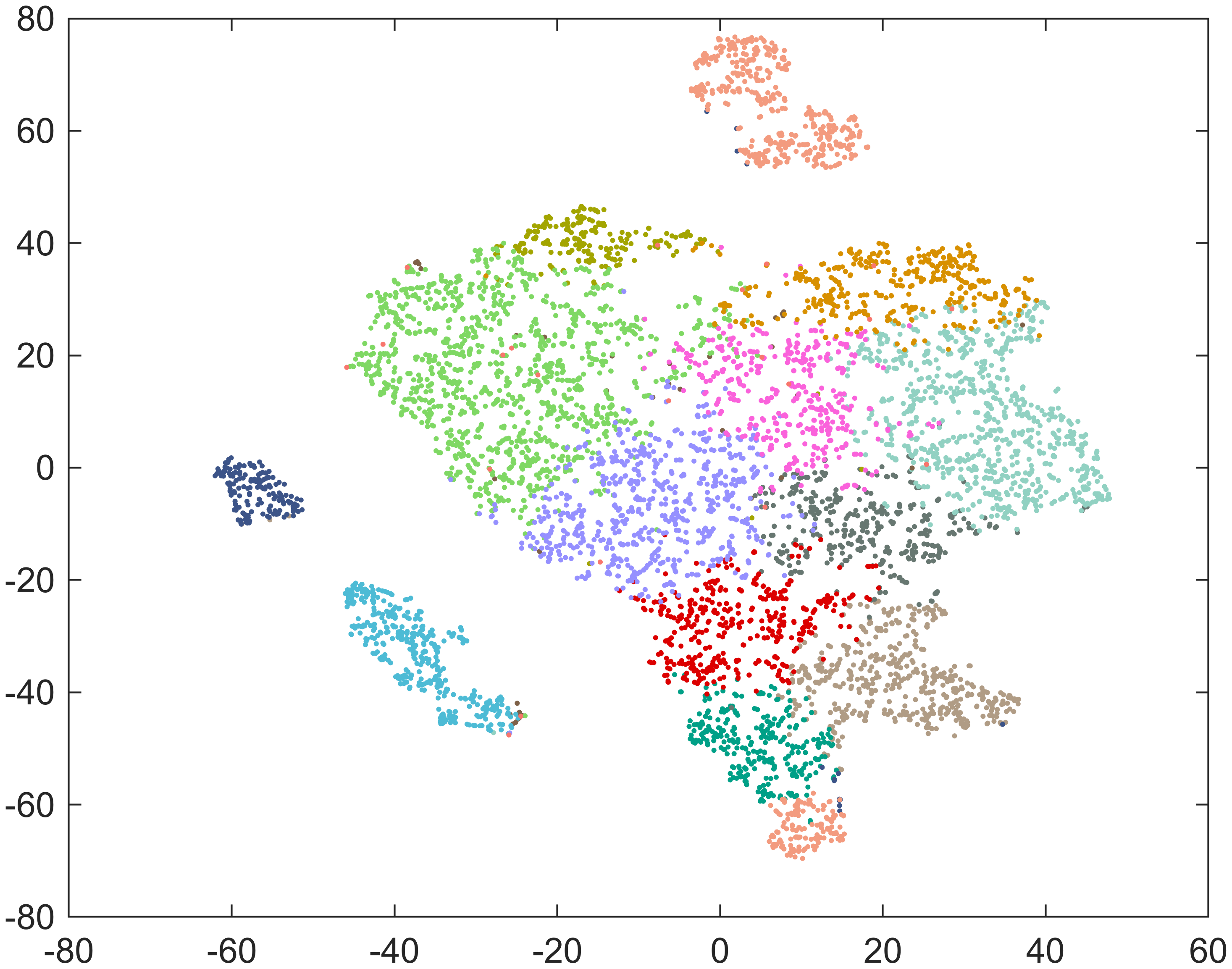
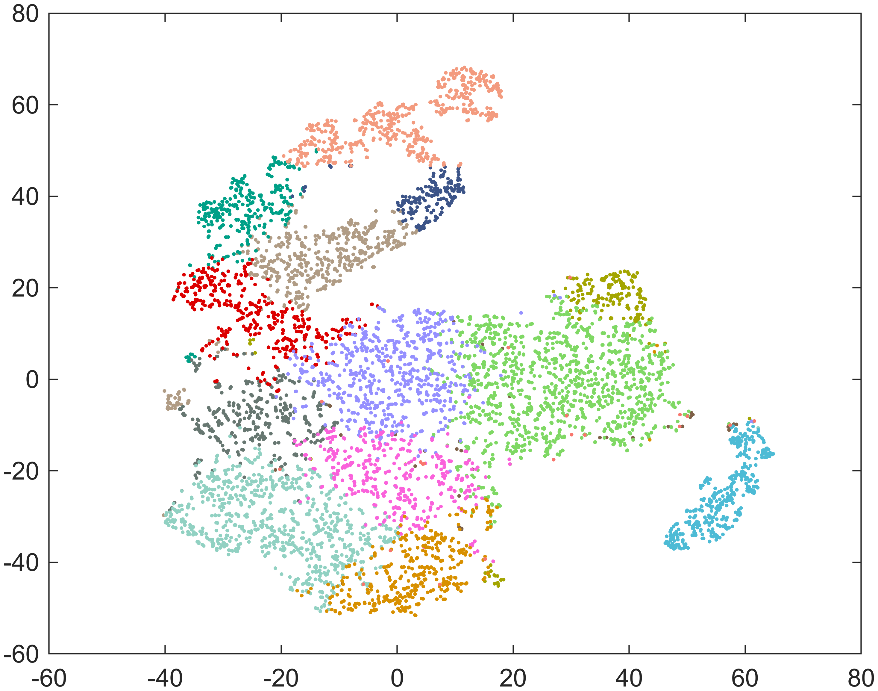
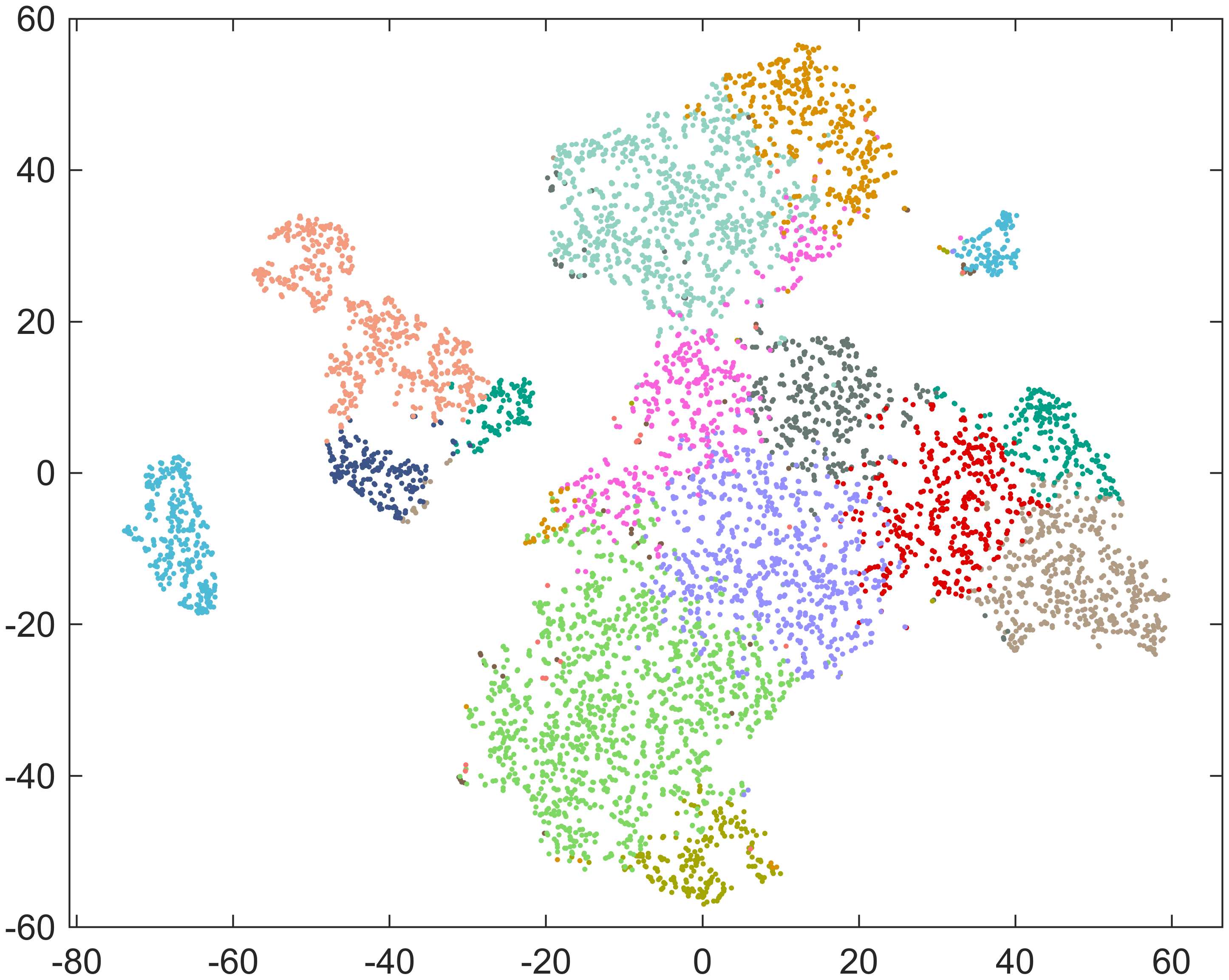
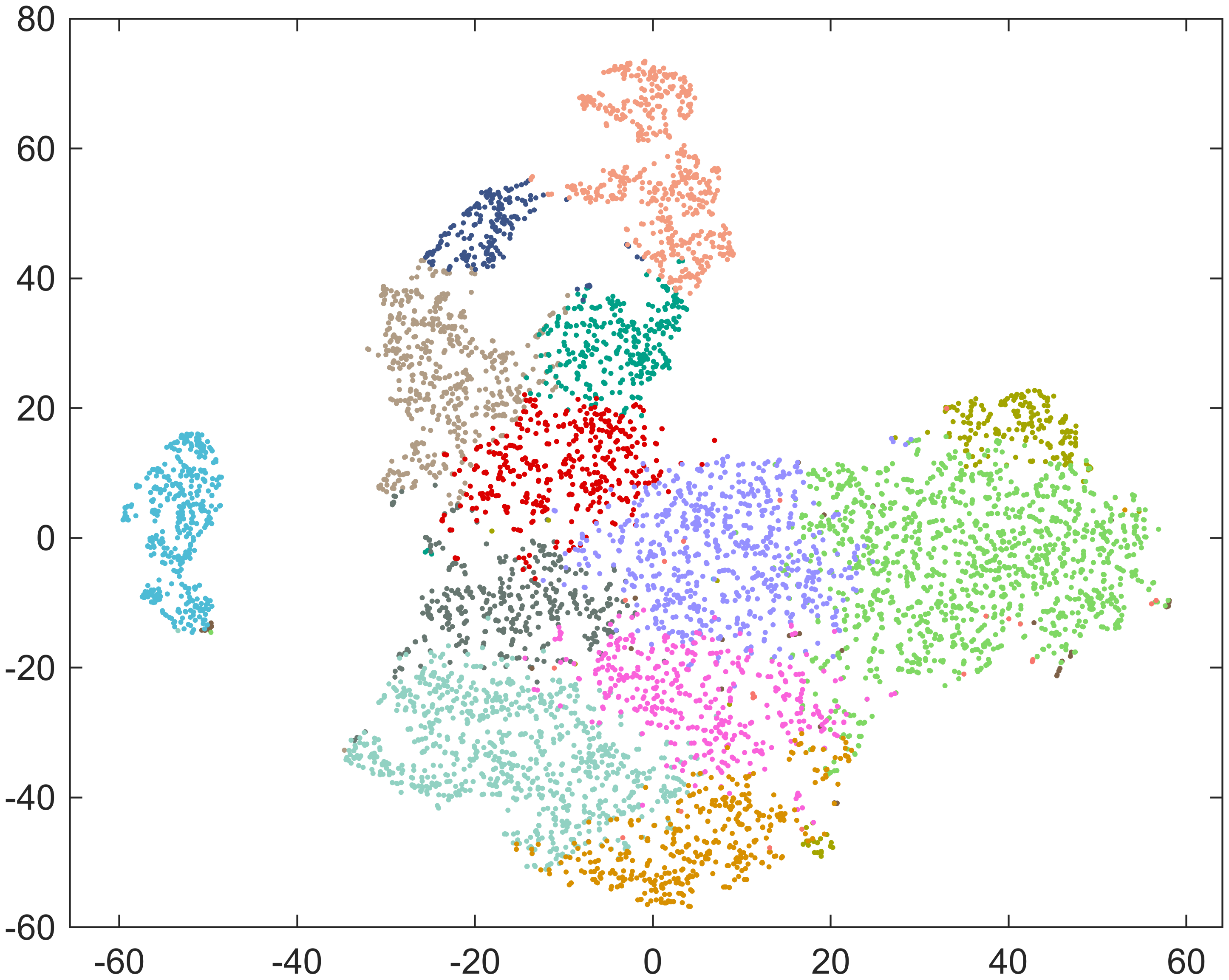
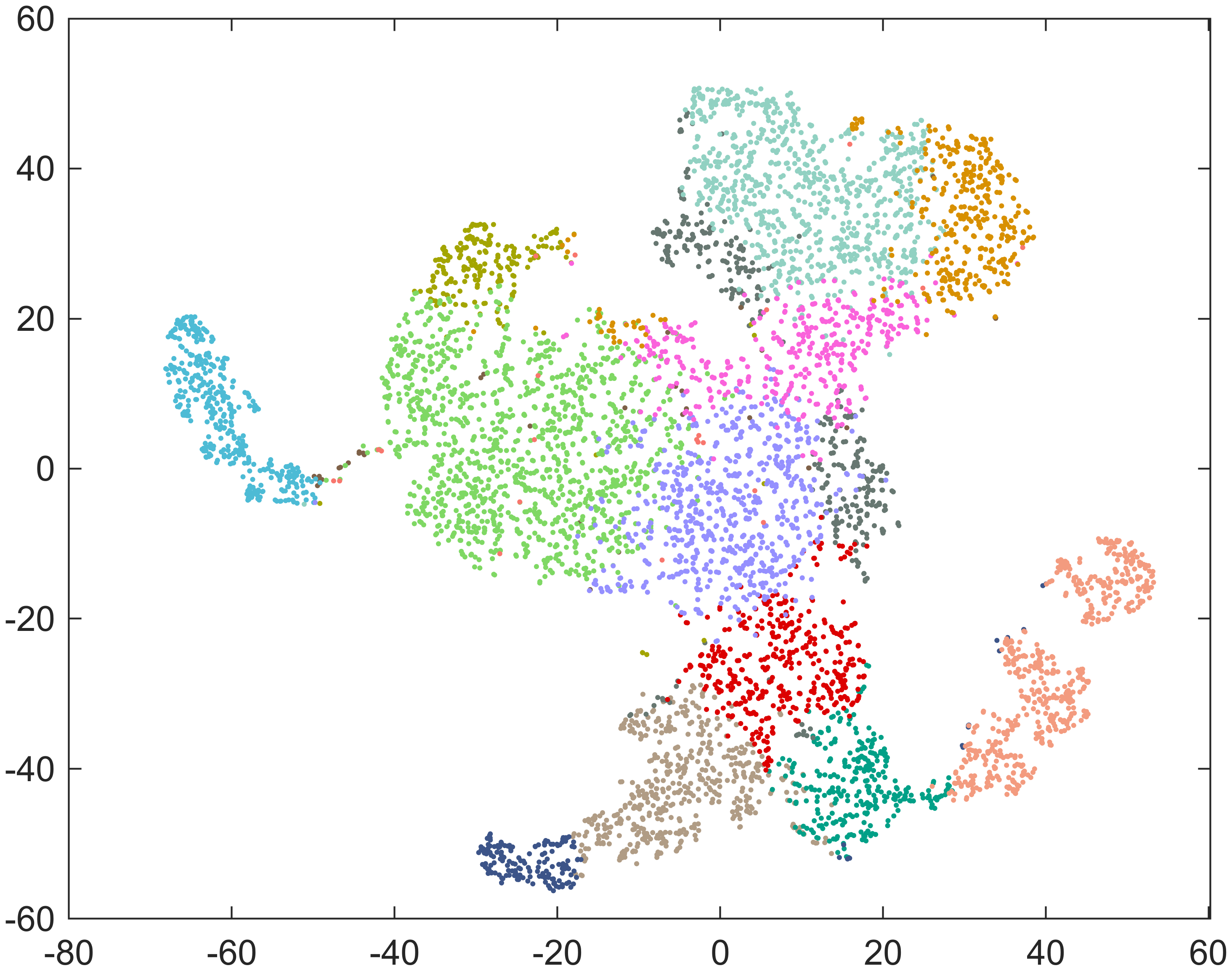
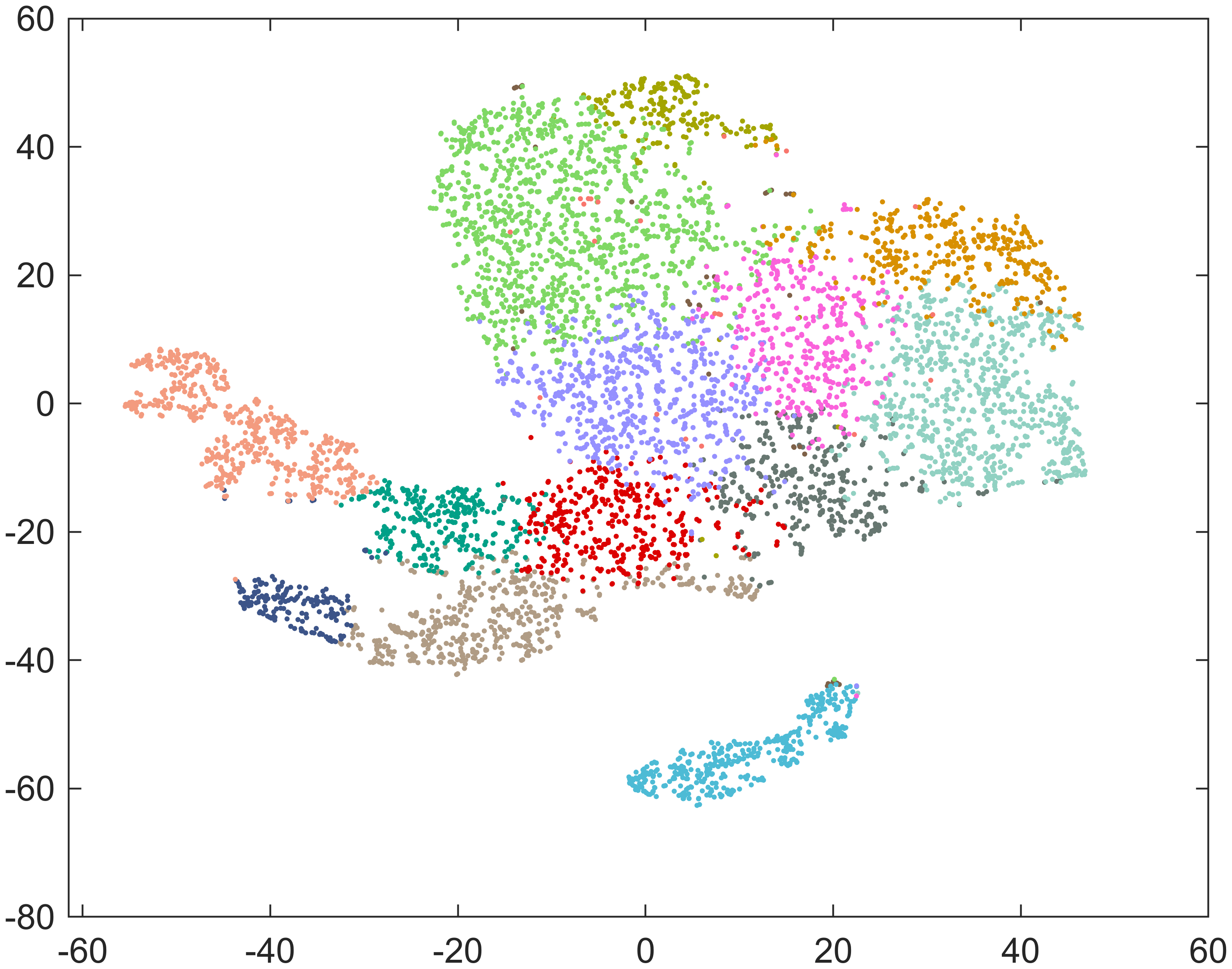
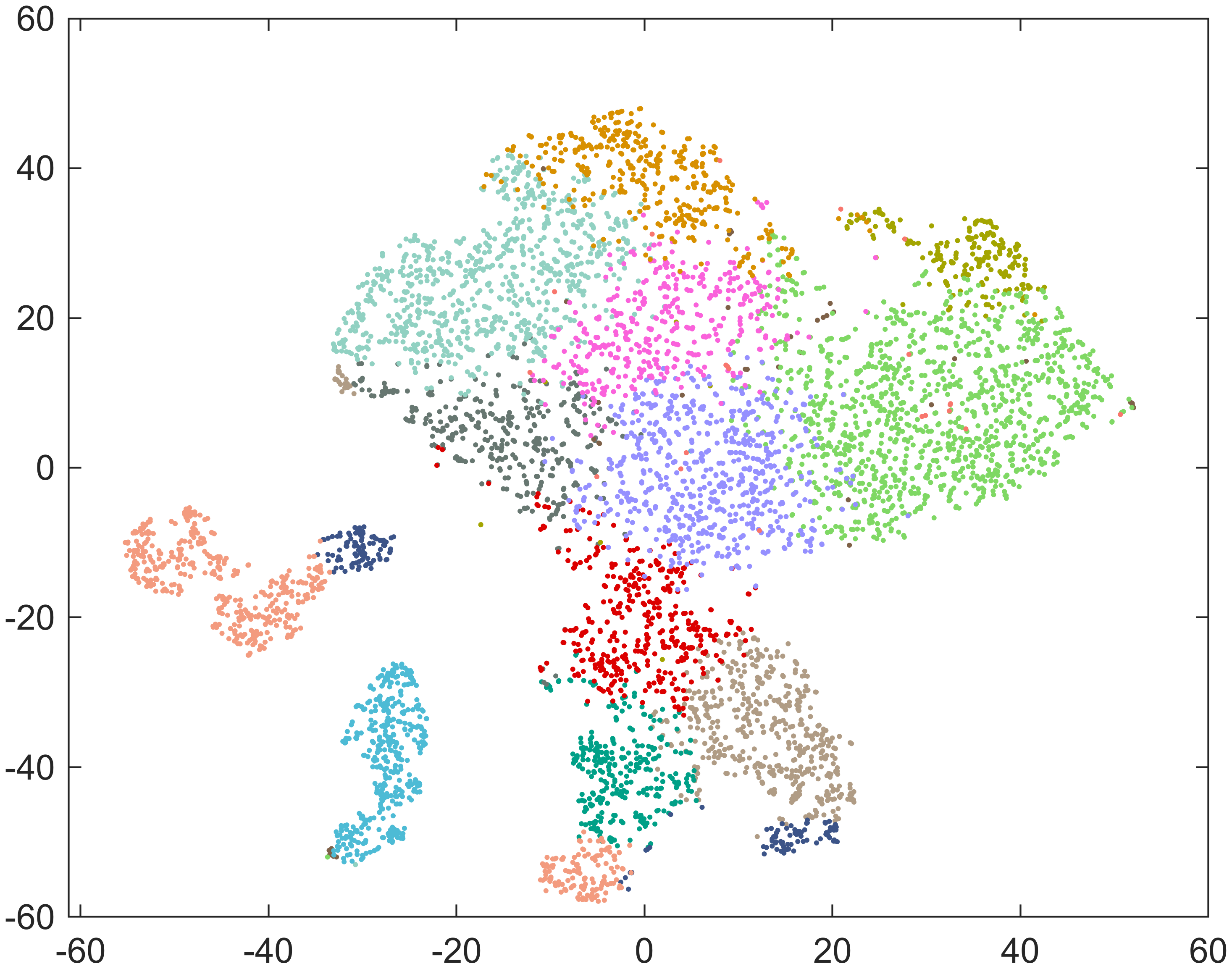
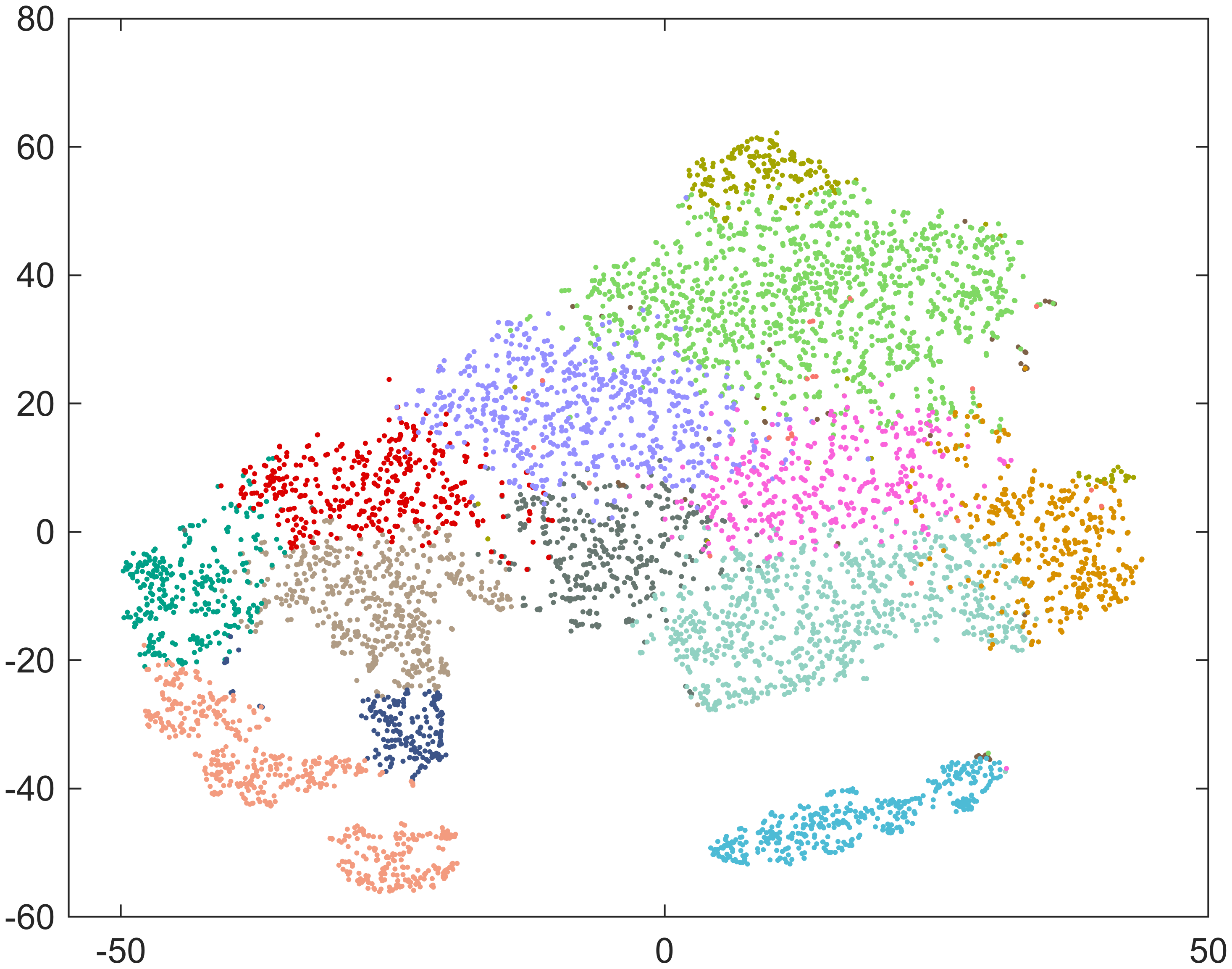
Figure A.3: Scatter plots for the two-dimensional t-distributed stochastic neighbour embedding of the result from the principal nested spheres with $d=1,\dots,12$ in (a)–(l).

A.4 Algorithms for fitting the principal nested submanifolds

Algorithm 1 An algorithm for the principal nested submanifolds

The noisy data set $\mathcal{Y}=\{y_{1},\dots,y_{n}\}\subset\mathbb{R}^{D}$, the radius parameter $r$, embedding set $\mathcal{E}\subset\mathbb{R}^{D^{\prime}}$

$\mathcal{X}_{D}=\{x_{1},\dots,x_{n}\}\leftarrow$ embedding of $\mathcal{Y}$ in $\mathcal{E}$

for $x_{i}$ in $\mathcal{X}_{D}$ do

  Calculate $\{\widehat{\Pi}_{r,i,1},\dots,\widehat{\Pi}_{r,i,D^{\prime}}\}$ with $(x_{i},\ \mathcal{X}_{D},\ r)$

end for

for $d=D-1:1$ do

  $\mathcal{X}_{d}\leftarrow$ projections of $\mathcal{X}_{d+1}$ on $\mathcal{M}_{d}$ with $\bigl{(}\mathcal{X}_{D},\ r,\ \{\widehat{\Pi}_{r,i,1},\dots,\widehat{\Pi}_{r,i,D^{\prime}-d}\}_{i=1}^{n}\bigl{)}$

  $\mathcal{Y}_{d}\leftarrow$ map $\mathcal{X}_{d}$ back to $\mathbb{R}^{D}$

end for

$\{\mathcal{Y}_{1},\dots,\mathcal{Y}_{D-1}\}$

Algorithm 2 Project a point $z$ onto $\mathcal{M}_{d}$

The point to project $z$, the noisy data set $\mathcal{X}_{D}=\{x_{1},\dots,x_{n}\}$, the radius parameter $r$, the collection of projection matrices at each point in $\mathcal{X}_{D}$, $\{\widehat{\Pi}_{r,i,1},\dots,\widehat{\Pi}_{r,i,D^{\prime}-d}\}_{i=1}^{n}$, the embedding set $\mathcal{E}$

for $\text{iter}=1$: MaxIter do

  $\alpha_{i}(z)\leftarrow$ calculate weights defined in (3) with $(z,\ \mathcal{X}_{D},\ r)$

  $\Delta_{z}\leftarrow\sum\alpha_{i}(z)x_{i}-z$

  $F_{z}\leftarrow 0$

  for $t=1$ to $D^{\prime}-d$ do

   $\widehat{\Pi}_{z}^{(t)}\leftarrow\mathds{P}_{1}\left(\sum\alpha_{i}(z)\Pi_{i}^{(t)}\right)$

   $F_{z}\leftarrow F_{z}+\widehat{\Pi}_{r,i,t}\Delta_{z}$

  end for

  if $\|F_{z}\|<\epsilon$ then

   break

  end if

  $z\leftarrow z+F_{z}$

end for

$z\leftarrow\operatorname*{arg\,min}_{z^{\prime}\in\mathcal{E}}\|z-z^{\prime}\|$

$z$

References

- Pearson [1901] Karl Pearson. Liii. on lines and planes of closest fit to systems of points in space. The London, Edinburgh, and Dublin Philosophical Magazine and Journal of Science, 2(11):559–572, 1901.
- Hotelling [1933] Harold Hotelling. Analysis of a complex of statistical variables into principal components. Journal of Educational Psychology, 24(6):417–441, 1933.
- Hotelling [1936] Harold Hotelling. Simplified calculation of principal components. Psychometrika, 1(1):27–35, 1936.
- Girshick [1936] Meyer Abraham Girshick. Principal components. Journal of the American Statistical Association, 31(195):519–528, 1936.
- Girshick [1939] Meyer Abraham Girshick. On the sampling theory of roots of determinantal equations. The Annals of Mathematical Statistics, 10(3):203–224, 1939.
- Anderson [1963] Theodore Wilbur Anderson. Asymptotic theory for principal component analysis. The Annals of Mathematical Statistics, 34(1):122–148, 1963.
- Tenenbaum et al. [2000] Joshua B Tenenbaum, Vin de Silva, and John C Langford. A global geometric framework for nonlinear dimensionality reduction. Science, 290(5500):2319–2323, 2000.
- Roweis and Saul [2000] Sam T Roweis and Lawrence K Saul. Nonlinear dimensionality reduction by locally linear embedding. Science, 290(5500):2323–2326, 2000.
- Zhang and Zha [2004] Zhenyue Zhang and Hongyuan Zha. Principal manifolds and nonlinear dimensionality reduction via tangent space alignment. SIAM Journal on Scientific Computing, 26(1):313–338, 2004.
- van der Maaten and Hinton [2008] Laurens van der Maaten and Geoffrey Hinton. Visualizing data using t-sne. Journal of Machine Learning Research, 9(86):2579–2605, 2008.
- McInnes et al. [2018] Leland McInnes, John Healy, and James Melville. Umap: Uniform manifold approximation and projection for dimension reduction. arXiv preprint arXiv:1802.03426, 2018.
- Donnell et al. [1994] Deborah J Donnell, Andreas Buja, and Werner Stuetzle. Analysis of additive dependencies and concurvities using smallest additive principal components. The Annals of Statistics, 22(4):1635–1668, 1994.
- Panaretos et al. [2014] Victor M Panaretos, Tung Pham, and Zhigang Yao. Principal flows. Journal of the American Statistical Association, 109(505):424–436, 2014.
- Yao et al. [2026] Zhigang Yao, Benjamin Eltzner, and Tung Pham. Principal sub-manifolds. Statistica Sinica, 36(3):1–41, 2026.
- Jung et al. [2012] Sungkyu Jung, Ian L Dryden, and James Stephen Marron. Analysis of principal nested spheres. Biometrika, 99(3):551–568, 2012.
- Eltzner et al. [2018] Benjamin Eltzner, Stephan Huckemann, and Kanti V. Mardia. Torus principal component analysis with applications to RNA structure. The Annals of Applied Statistics, 12(2):1332–1359, 2018.
- Fefferman et al. [2018] Charles Fefferman, Sergei Ivanov, Yaroslav Kurylev, Matti Lassas, and Hariharan Narayanan. Fitting a putative manifold to noisy data. In Conference on Learning Theory, pages 688–720. PMLR, 2018.
- Fefferman et al. [2021] Charles Fefferman, Sergei Ivanov, Matti Lassas, and Hariharan Narayanan. Fitting a manifold of large reach to noisy data. arXiv:1910.05084, 2021.
- Yao and Xia [2019] Zhigang Yao and Yuqing Xia. Manifold fitting under unbounded noise. arXiv preprint arXiv:1909.10228, 2019.
- Yao et al. [2023a] Zhigang Yao, Jiaji Su, Bingjie Li, and Shing-Tung Yau. Manifold fitting. arXiv preprint arXiv:2304.07680, 2023a.
- Yao et al. [2023b] Zhigang Yao, Yuqing Xia, Do Van Tran, and Zhenyue Zhang. Hunting principal sub-manifolds: new theories and methods. Technical Report, 2023b.
- Huckemann and Ziezold [2006] Stephan Huckemann and Herbert Ziezold. Principal component analysis for Riemannian manifolds, with an application to triangular shape spaces. Advances in Applied Probability, 38(2):299–319, 2006.
- Huckemann et al. [2010] Stephan Huckemann, Thomas Hotz, and Axel Munk. Intrinsic shape analysis: Geodesic PCA for Riemannian manifolds modulo isometric lie group actions. Statistica Sinica, 20(1):1–58, 2010.
- Federer [1959] Herbert Federer. Curvature measures. Transactions of the American Mathematical Society, 93(3):418–491, 1959.
- Niyogi et al. [2008] Partha Niyogi, Stephen Smale, and Shmuel Weinberger. Finding the homology of submanifolds with high confidence from random samples. Discrete & Computational Geometry, 39(1):419–441, 2008.
- Haber et al. [2017] Adam L Haber, Moshe Biton, Noga Rogel, Rebecca H Herbst, Karthik Shekhar, Christopher Smillie, Grace Burgin, Toni M Delorey, Michael R Howitt, Yarden Katz, et al. A single-cell survey of the small intestinal epithelium. Nature, 551(7680):333–339, 2017.
- Rosvall and Bergstrom [2008] Martin Rosvall and Carl T Bergstrom. Maps of random walks on complex networks reveal community structure. Proceedings of the National Academy of Sciences, 105(4):1118–1123, 2008.
- Lee [2012] John M Lee. Smooth manifolds. Springer, 2012.