Absolute frequency measurement of the ¹S₀ - ³D₁ transition of ¹⁷⁶Lu⁺ via link to international atomic time

Abstract

We report an absolute frequency measurement of the ${}^{1}\rm S_{0}$ to ${}^{3}\rm D_{1}$ optical clock transition in ${}^{176}{\rm Lu}^{+}$. Traceability to the International System of Units (SI) is realized by remote link to International Atomic Time. The measurement result is $353\,638\,794\,073\,800.34(32)$Hz, a fractional uncertainty of $9.1\times 10^{-16}$. The result was obtained by operating a single-ion ${}^{176}{\rm Lu}^{+}$ frequency standard intermittently over 3 months with total uptime of 162 hours. This is the first reported absolute frequency value for the ${\rm Lu}^{+}\,(^{3}\rm D_{1})$ optical standard.

Keywords: frequency standards, lutetium ion, optical clock, international atomic time

1 Introduction

The International System of Units (SI) defines the second by the duration of a fixed number of oscillation periods of the caesium (${}^{133}\rm Cs$) ground-state hyperfine transition. The best primary frequency standards (PFS) to realize the SI second are Cs fountains with an inaccuracy near one part in $10^{-16}$  [1, 2]. Several frequency standards based on optical transitions of different ions and atoms now report uncertainties near one part in $10^{-18}$  [3, 4, 5, 6, 7, 8] and a roadmap to the redefinition of the SI second as been devised [9]. The International Committee for Weights and Measures (CIPM) already maintains a list of recommended values for standard frequencies, many recognized as secondary representations of the second (SRS). Some optical clocks based on SRS reference transitions are officially recognized as secondary frequency standards (SFS) and in recent years contribute to the steering of International Atomic Time (TAI) through reporting of measurements to the International Bureau of Weights and Measures (BIPM). For a recently established optical clock species such a Lu⁺, absolute frequency measurements are necessary for CIPM to establish a recommended value and which are prerequisite to becoming a SRS.

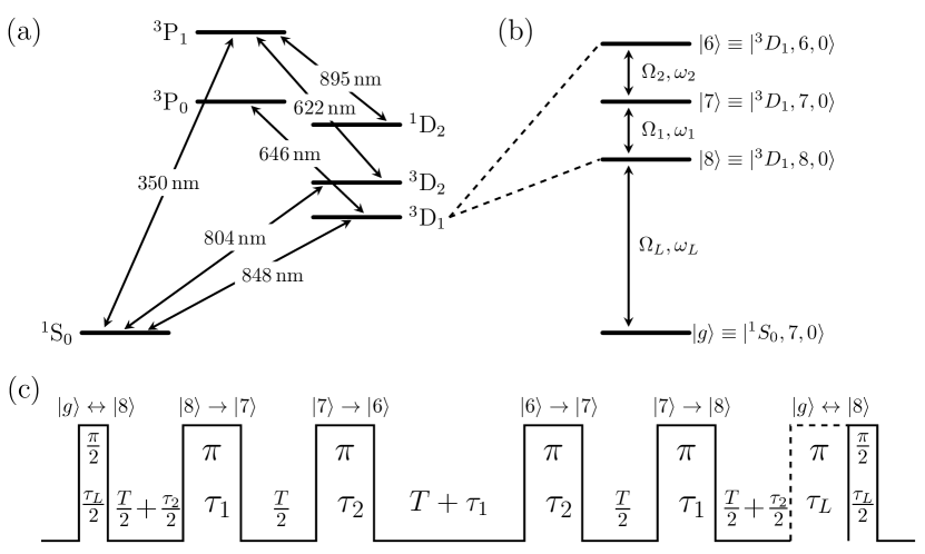
Figure 1: (a) Energy level structure of ${}^{176}\mathrm{Lu}^{+}$. (b) Microwave and optical transitions used in the clock interrogation sequence. (c) Clock interrogation sequence for hyperfine averaging with hyper-Ramsey spectroscopy.

The ${}^{1}\rm S_{0}-^{3}\rm D_{1}$ transition of ${}^{176}{\rm Lu}^{+}$ is an especially promising reference frequency for which $\lesssim 10^{-18}$ uncertainty can be realized with relative ease [8]. Here we report the first frequency measurement of the Lu⁺(³D₁) optical standard. In section 2, we outline the ${}^{176}{\rm Lu}^{+}$ clock operation and the frequency measurement scheme to link to the SI second. In section 3 we detail the frequency shifts and uncertainties for the ${\rm Lu}^{+}$ clock. In section 4, we analyze the uncertainty contributions from each step of the frequency chain. Finally we discuss results in section 5.

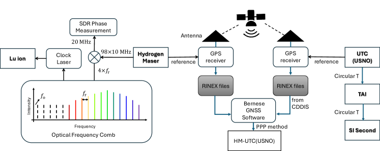
Figure 2: GPS link to the SI second.

2 Experimental System and Methods

2.1 ${}^{176}{\rm Lu}^{+}$ optical frequency standard

For ${}^{176}\mathrm{Lu}^{+}$ hyperfine averaging is used to realize an effective $J=0$ level which practically eliminates second-order Zeeman shifts, and shifts arising from rank 2 tensor interactions, such as the electric quadrupole moment [10]. The reference frequency, $f_{\mathrm{Lu}}$, of ${\rm Lu}^{+}\,(^{3}\rm D_{1})$ standard is thus defined as the average of the three optical transitions from $|\,g\,\rangle\equiv|\,^{1}S_{0},7,0\,\rangle$ to the hyperfine states $|\,F\,\rangle\equiv|\,^{3}D_{1},F,0\,\rangle$ where $F=6,7,$ and $8$. This average can be conveniently realized using a hybrid microwave and optical interrogation [11]. As illustrated in figure 1(b-c), the interrogation sequence consists of an optical Ramsey interrogation on the $|\,g\,\rangle\leftrightarrow|\,8\,\rangle$ transition, where additional microwave pulses transfer population between the hyperfine states during the interrogation time. Their timing is chosen such that the effective time in each of the hyperfine states is the same. When the laser is servoed to the central fringe of the resulting Ramsey spectrum, the hyperfine-averaged (HA) clock frequency is given by

$$f_{\mathrm{Lu}}=\frac{1}{3}(\nu_{8}+\nu_{7}+\nu_{6})=\nu_{L}+\frac{1}{3}(2f_{1}+f_{2}),$$ (1)

where $\nu_{F}$ is the resonant frequency of the $|\,g\,\rangle\leftrightarrow|\,F\,\rangle$ optical transition, $\nu_{L}=\omega_{L}/(2\pi)$ is the laser frequency, and $f_{k}=\omega_{k}/(2\pi)$ for $k=1,2$ are the microwave frequencies used within the interrogation sequence. As explained in previous work [8, 11], the interrogation sequence ensures $\nu_{L}+(2f_{1}+f_{2})/3$ represents the HA clock frequency, as indicated by Eq. 1, even if the microwave fields are not exactly resonant.

Experiments are performed with a single ${}^{176}\mathrm{Lu}^{+}$ ion in a linear Paul trap which has been described previously in  [8, 12], denoted as Lu-2. Figure 1 shows the energy levels and transitions relevant for laser cooling, trapping, and state manipulation. Each experiment starts with Doppler cooling on the 646 nm transition followed by preparation in the $|\,^{3}D_{1},8,0\,\rangle$ state and then the Ramsey interrogation sequence as shown in figure 1(c). The timing parameters used for the Ramsey interrogation are $\tau_{\mathrm{L}}=1.4\,\,\mathrm{ms}$, and $\tau_{1}=\tau_{2}=2\,\,\mathrm{ms}$ with total Ramsey interrogation time $T_{\mathrm{R}}=3(T+\tau_{1}+\tau_{2})=42\,\,\mathrm{ms}$. The additional 848-nm $\pi$ pulse, indicated by the dashed line in figure 1(c), is phase shifted by 180 degrees and included for suppressing the probe induced ac Stark shift by the hyper-Ramsey method [13, 14]. A frequency discriminator for locking to the central Ramsey fringe is generated by repeating the entire sequence twice per cycle, alternating the phase shift on the first $\pi/2$ pulse by $\pm{90}$ degrees. Every $t_{u}=3.6$ seconds, after $N=25$ cycles, the 848 nm laser frequency is steered to maintain the condition given by (1).

The microwave frequencies $f_{1}$ and $f_{2}$ remain fixed throughout all measurements. All synthesized rf offsets and the microwave frequencies are referenced to a hydrogen maser (Microchip MHM-2010).

The 848 nm clock laser is an external cavity diode laser stabilized to a high finesse ($\sim 400000$) optical reference cavity with a 10-cm ultra low expansion (ULE) glass spacer. This cavity is under vacuum and actively temperature stabilized to its zero coefficient of thermal expansion point at 33.2 ^∘C. An rf offset generated by a direct digital synthesizer (DDS) continuously compensates the long term linear creep of the ULE cavity of 40 mHz s^-1. An instability of $1.5\times 10^{-15}$ at 1 second was measured in a three-corner hat measurement against two additional optical reference cavities. During Lu⁺ servo operation, the fractional frequency instability is quantum projection noise limited to

$$\sigma(\tau)=\frac{1}{f_{\mathrm{Lu}}}\frac{1}{2\pi CT_{R}\sqrt{2N}}\sqrt{\frac{t_{u}}{\tau}}\approx\frac{3.9\times 10^{-15}}{\sqrt{\tau}},$$

for averaging time $\tau\gg t_{u}$ (in seconds). Here $C\approx 0.75$ is the Ramsey fringe contrast at $T_{R}=42$ ms.

As illustrated in figure 2, the optical clock laser frequency is compared to the hydrogen maser (HM) reference frequency, $f_{\mathrm{HM}}=10\,\,\mathrm{MHz}$, using a commercial Er-doped femtosecond fiber frequency comb (Menlo Systems). The $\sim$250 MHz repetition rate ($f_{\mathrm{r}}$) is referenced to the ${}^{176}\mathrm{Lu}^{+}$ stabilized clock laser by phase locking the beat note between the laser and comb to a DDS. The carrier-envelope offset frequency of the comb, $f_{\mathrm{o}}$, is phase locked to the HM. The HM signal is multiplied up to $980\,\,\mathrm{MHz}$ using a phase locked dielectric resonator oscillator and mixed with the fourth harmonic of $f_{r}$ at 1 GHz. The phase of the down mixed signal at 20 MHz is measured continuously with zero dead-time using software defined radio (SDR) hardware (USRP N210) [15]. The SDR measurement system contributes uncertainty of $3\times 10^{-14}\,(\tau/\mathrm{s})^{-1}$ to the measurement of $\frac{f_{\mathrm{Lu}}}{f_{\mathrm{HM}}}$ for averaging time $\tau$.

2.2 Link to SI second

The system to link the optical clock to the SI second is outlined in figure 2. Traceability to the SI second is achieved by a link to International Atomic Time (TAI), which differs from Coordinated Universal Time (UTC) by an integer number of leap seconds, but shares the same scale interval. UTC is a virtual timescale with local realisations, UTC($k$), at laboratories reporting to BIPM. Since a local realization is not directly available in our lab, we rely on a GPS link to a UTC($k$) realized in a remote laboratory [16]. Specifically we choose UTC(USNO) because it has good stablity and GPS receiver data is freely available. The data from GPS receiver USN7, which is referenced to UTC(USNO) [17] is obtained from CDDIS [18, 19] in Receiver Independent Exchange (RINEX) format. Local RINEX files are generated by a dual-band GNSS receiver (PolaRx5TR) referenced to the HM. A Precise Point Positioning (PPP) algorithm [20, 21] is implemented using the Bernese GNSS software [22] to evaluate the phase difference $\Delta x=x(\mathrm{HM})-x(\mathrm{USNO})$ on 30 s intervals. As shown in figure 3 (orange), the PPP link instability is observed to average down as $4.6\times 10^{-15}\,(\tau)^{-0.75}$ until reaching a $1.3\times 10^{-15}$ frequency flicker noise floor attributed to the HM at around 5 days. The PPP result is used to evaluate the HM frequency offset and drift referenced to UTC(USNO) over an 80 day interval encompassing the optical clock measurements. The HM acts as a flywheel for interpolation between optical clock operation.

Circular T data published by BIPM links UTC(USNO) to UTC, and thereby TAI, on five day intervals. TAI is a realisation of terrestrial time (TT), which is a coordinate time scale defined in the geocentric reference frame with the scale unit SI second on the geoid. The estimated deviation between TAI and TT is given by $y_{\mathrm{TAI}}=-d$ where $d$ is published in part 3 of the Circular T report for each month.

The complete frequency chain is summarized as

$$\frac{f_{\mathrm{Lu}}}{f_{\mathrm{SI}}} =\frac{f_{\mathrm{Lu},T_{1}}}{f_{\mathrm{HM},T_{1}}}\times\frac{f_{\mathrm{HM},T_{1}}}{f_{\mathrm{HM},T_{2}}}\times\frac{f_{\mathrm{HM},T_{2}}}{f_{\mathrm{UTC(USNO)},T_{2}}}$$ (2)

$$\times\frac{f_{\mathrm{UTC(USNO)},T_{2}}}{f_{\mathrm{TAI},T_{2}}}\times\frac{f_{\mathrm{TAI},T_{2}}}{f_{\mathrm{TAI},T_{3}}}\times\frac{f_{\mathrm{TAI},T_{3}}}{f_{\mathrm{SI},T_{3}}}$$

where $T_{1}$ corresponds to the uptime intervals of the Lu⁺ frequency standard, $T_{2}$ and $T_{3}$ are the 5-day and 1-month intervals aligned to the Circular T respectively. The ratios ${f_{\mathrm{HM},T_{1}}}/f_{\mathrm{HM},T_{2}}$ and ${f_{\mathrm{TAI},T_{2}}}/{f_{\mathrm{TAI},T_{3}}}$ account for the uncertainty in interpolation of the HM and TAI respectively.

3 Lu⁺ Systematics

Here we discuss only systematics shifts $>10^{-17}$ which are of statistical significance to the absolute frequency measurement. This includes only the quadratic Zeeman shift and gravitational redshift. For this apparatus (Lu-2) all other systematic shifts and uncertainties are evaluated to be below $2\times 10^{-18}$  [8] . Excess micromotion was measured in three orthogonal directions on three occasions throughout the measurement campaign and in each instance the corresponding second-order Doppler shift was $<2\times 10^{-19}$ before (re-)optimizing the compensation.

3.1 Quadratic Zeeman

A residual quadratic Zeeman shift remains after hyperfine averaging due to hyperfine-mediated mixing between fine structure levels. The quadratic Zeeman coefficient has been measured to be -4.89264(88) Hz/mT² [8]. Measurement of the linear Zeeman splitting on the $|\,^{3}D_{1},6,0\,\rangle$ to $|\,^{3}D_{1},6,\pm 1\,\rangle$ microwave transition is regularly interleaved during clock operation from which the magnetic field at the ion is inferred via the g-factor $g_{6}=-0.071\,662\,506(33)$ reported in [23]. The magnetic field was passively stable near 0.100 mT with 2 $\mu$T standard deviation over the full campaign. The corresponding quadratic Zeeman shift is 48.9(2.0) mHz, or $-1.38(5)\times 10^{-16}$ fractionally.

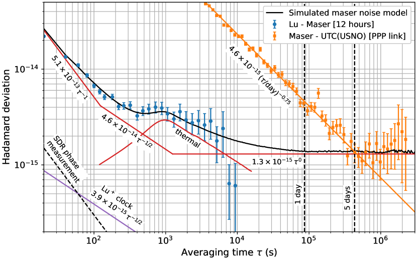
Figure 3: HM instability observed relative to the Lu⁺ clock from 12 hours continuous measurement (blue circles) and relative to UTC(USNO) via the PPP link (orange squares). The black line is the numerical implementation of the noise model for the HM which is generated as the sum of noise processes for which the individual contributions are indicated by the red lines.

3.2 Gravitational redshift

The redshift is given by $\frac{\Delta f}{f}=\frac{gh}{c^{2}}$ where $g=9.7803(3)\,\mathrm{m}~\mathrm{s}^{-2}$ is the local gravitational acceleration and the geoid height $h=H-N$ is obtained from the difference in the orthonormal height $H$ and geoid undulation $N$. The orthonormal height of the trapped Lu⁺ ion from the earth ellipsoid (WGS84) was measured to be $H=23.68(10)$ m by orthometric height leveling relative to the rooftop GNSS antenna. A geoid undulation of $N=7.89(10)$ m is obtained from the Earth Gravitational Model (EGM2008). The gravitational redshift is estimated to be 1.72(4)$\times 10^{-15}$, including additional uncertainty to allow for bias due to tidal modulation [24].

4 Analysis of link to SI second

Measurements of the ¹⁷⁶Lu⁺ frequency standard relative to the local hydrogen maser, $f_{\mathrm{Lu}}/f_{\mathrm{HM}}$, were taken between the modified Julian dates (MJD) 59270 and 59338, spanning March to May in the year 2021. The total measurement uptime was 162 hours, where the average length of a single continuous run was 2.9 hours. The analysis follows equation (2) and is carried out in four steps. First the maser drift and frequency offset are evaluated by the GPS link and subtracted from the local measurements. Second the measurements are averaged over 5-day intervals aligned to the Circular T, accounting for the uncertainty due to interpolation over dead times using the hydrogen maser as a flywheel. Third, the 5 day averages are linked to TAI by the Circular T with weighted averages evaluated for each month. Five day intervals without optical frequency measurements are considered dead time and an interpolation uncertainty using TAI as the flywheel is estimated. Finally, monthly averages are linked to SI by the Circular T.

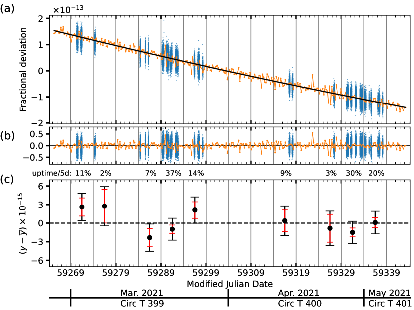
Figure 4: (a) Evaluation of the HM drift over an 80 day interval. The blue points are the intermittent measurements of the maser relative to the optical clock as logged at 20 second intervals. Orange points are the HM deviation measured against UTC(USNO) via the PPP link, plotted as 6 hour averages. A quadratic fit (black line) models the frequency offset and drift of the HM relative to UTC(USNO). (b) After subtraction of the fitted maser drift and offset, blue points are the optical measurements relative to UTC(USNO) and orange points are the HM-UTC(USNO) residual. (c) Black points are the measurements $y[f_{\mathrm{Lu}}/f_{\mathrm{TAI}}]$ on 5-day intervals aligned to the Circular T reports. Outer black error bars represent the total statistical uncertainty, and inner red error bars are the uncertainty contribution only from dead time interpolation. The reduced chi-squared is $\chi^{2}_{\nu}=0.67$ with $\nu=8$ degrees of freedom.

4.1 Maser drift

The hydrogen maser drift is evaluated relative to UTC(USNO) over an 80 day interval encompassing the optical frequency measurements, as shown in figure 4. Over this interval the maser frequency drift slightly deviates from linear so a quadratic model is used. The maser linear drift over this is interval is near $-3.7\times 10^{-15}\,\mathrm{d}^{-1}$ and aging at a rate $4.6\times 10^{-15}\,\mathrm{d}^{-1}\mathrm{year}^{-1}$. The fitted maser drift model is subtracted from the local observations, the blue points in figure 4(a), to link the measurements to UTC(USNO) up to uncertainty from the additional noise process on the maser frequency which are assumed to have zero mean. The blue points in figure 4(b), which are $-y(\mathrm{Lu}/\mathrm{UTC(USNO)})$, are binned in 5 day intervals aligned to Circular T and averaged. The uncertainty in the 5 d averages of $y(\mathrm{Lu}/\mathrm{UTC(USNO)})$ has three contributions. First, the statistical uncertainty in the five day averages of $f_{\mathrm{HM}}/f_{\mathrm{UTC(USNO)}}$ relative to the maser drift model fit on the the 80 day interval. This is estimated to be $1.5\times 10^{-15}$ from the instability of the residuals, the orange points in figure 4(b), at five days, and is consistent with the Hadamard deviation of $f_{\mathrm{HM}}/f_{\mathrm{UTC(USNO)}}$ which is shown in figure 3. Second, the fitted drift model contributes uncertainty which is correlated across all measurements, and is estimated to contribute $2\times 10^{-16}$ to the final result. Third, the uncertainty from measurement dead time which is evaluated in the following section.

4.2 Dead time uncertainty

The dead time uncertainty is calculated by simulation of the maser noise [25, 26]. A maser noise model is constructed to be consistent with both the observed $f_{\mathrm{Lu}}/f_{\mathrm{HM}}$ instability on shorter timescales, and the maser flicker noise floor inferred from GPS link to UTC(USNO) on longer times scales. The allan deviation for the longest continuous measurement of $f_{\mathrm{Lu}}/f_{\mathrm{HM}}$ (12 h) is shown in figure 3. The noise model is the sum of white phase noise $5.1\times 10^{-13}\,(\tau/\mathrm{s})^{-1}$, white frequency noise $4.6\times 10^{-14}\,(\tau/\mathrm{s})^{-1/2}$, flicker frequency noise $1.3\times 10^{-15}$, and the bandwidth limited noise labeled ‘thermal’ in figure 3 which repoduces the instability plateau observed for averaging times $\lesssim 1\,\mathrm{h}$. We speculate the instability plateau observed to be due the thermal effects driven by the ambient temperature in lab, but we are not sure of the precise origin. It has however been consistently observed in $f_{\mathrm{Lu}}/f_{\mathrm{HM}}$ measurements over the last three years. The generated noise [27] is sampled to simulate $\sim 2\times 10^{3}$ trajectories on the interval $T_{2}=5\,\mathrm{d}$. For an uptime $T_{1}$, which may be distributed non-continuously over the interval $T_{2}$, the dead time uncertainty is calculated from the standard deviation of the difference in averages over $T_{1}$ and $T_{2}$. For the actual uptimes $T_{1}$ in the experimental data, the evaluated dead time uncertainties are shown as the black points in figure 5. The influence of the distribution of $T_{1}$ was further investigated by sampling random arrangements of $T_{1}$ as a function of total uptime fraction, with the restriction of a minimum (maximum) continuous experiment run time of 1 (12) hours to mimic typical operation. The gray shaded region in figure 5 bounds the maximum and minimum dead time uncertainty found under these criteria. The solid lines correspond to two special cases, $T_{1}$ as a single continuous run centered on $T_{2}$ (blue) and $T_{1}$ divided into five runs evenly spaced over the five days (orange). For future measurement campaigns this simulation can serve as a practical guide to determine the uptime fraction and dead-time distribution required to achieve a target uncertainty.

4.3 Diurnal effects

Correlations with a daily temperature cycle are of particular concern because the majority of the optical clock uptime was during the daytime. We analyzed all measurement residuals after maser drift subtraction for correlation with time of day acquired, but there is no definitive diurnal amplitude. Statistically, we can only bound the amplitude to $<1\times 10^{-15}$ and at this upper bound the final result would be biased by $5\times 10^{-16}$ when accounting for the distribution of uptime. We include this potential bias as a systematic uncertainty in the final result.

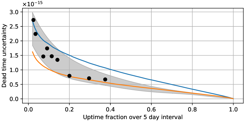
Figure 5: Estimated dead time uncertainty from simulation. Black points are simulated dead time uncertainty for the uptimes distributions present in the experimental data. See main text for description of other simulated results shown.

4.4 Link to TAI

The frequency ratio $f_{\mathrm{UTC(USNO)}}/f_{\mathrm{TAI}}$ is evaluated from the phase data reported on 5-day intervals in the Circular T reports [28]. The recommended link uncertainty for satellite frequency transfer is [29]

$$u=\frac{\sqrt{2}u_{\rm A}}{\tau_{0}}\left(\frac{\tau}{\tau_{0}}\right)^{-0.9},$$ (3)

where $u_{A}=0.2\,\mathrm{ns}$ is the satellite link phase instability for UTC(USNO) reported in the Circular T, $\tau_{0}=5\,$d, and here the measurement window $\tau$ is also 5 d.

The resulting fractional deviations $y[f_{\mathrm{Lu}}/f_{\mathrm{TAI}}]$ for each 5 day window are shown in figure 4(b) with all statistical uncertainty contributions summarized in table 1.

Table 1: Statistical uncertainty contributions to $f_{\mathrm{Lu}}/f_{\mathrm{TAI}}$ for each 5 day window.

MJD start	59269	59274	59284	59289	59294	59314	59324	59329	59334
MJD stop	59274	59279	59289	59294	59299	59319	59329	59334	59339
Lu uptime	11%	2%	7%	37%	14%	9%	3%	30%	20%
Ratio	Uncertainty $\times 10^{-16}$
HM interpolation	15	27	15	06.7	13	17	22	07.1	07.9
HM/UTC(USNO)	15	15	15	15	15	15	15	15	15
UTC(USNO)/TAI	06.6	06.6	06.6	06.6	06.6	06.6	06.6	06.6	06.6
Lu/TAI Total	22	32	22	17	21	24	27	18	18

4.5 Link to SI

The measurement intervals span three Circular T reports; 399, 400, and 401. We evaluate the weighted averages of the 5-day results falling within each approximately monthly report interval. The uncertainty from interpolation of TAI over the 5-day dead time intervals is estimated by simulation, similar to the HM interpolation. The stability of TAI is derived from the free atomic timescale (Echelle Atomique Libre, EAL), and an instability model is reported for each Circular T [30]. For all three reports the model is given to be the sum of $1.4\times 10^{-15}(\tau/\mathrm{s})^{-1/2}$ white frequency noise, $2\times 10^{-16}$ flicker frequency noise, and $2\times 10^{-17}(\tau/\mathrm{s})^{1/2}$ random walk frequency noise.

The Circular T reports the fractional deviation of the TAI scale interval relative the SI second as $d$ and its total uncertainty $u$. The estimation of $d$ is based on all primary and secondary frequency standard (PSFS) measurements contributing to TAI steering. Following the procedure reported by others [25, 31], the total uncertainty $u$ is separated into a statistical component and systematic component using the systematic uncertainties of the individual PSFS reported as $\mu_{B}$ in the Circular T. For the three Circular T reports spanned, most of the clocks reporting are the same for all three months and so the total systematic component is assumed to be correlated. The uncertainty budget for each month and the final result are summarized in table 2.

Table 2: Uncertainty budget for the absolute frequency measurement of the ${}^{176}\mathrm{Lu}^{+}$ ${}^{1}\rm S_{0}-{{}^{3}}\rm D_{1}$ clock transition for each month, and the total campaign. All uncertainties given in $10^{-16}$ fractional frequency uncertainty.

	Cir.T	Cir.T	Cir.T
	399	400	401	Total
	Statistical uncertainty
Lu/TAI	09.7	13	18	07.1
TAI interpolation	01.7	02.9	06.3	01.5
TAI/SI	00.7	00.7	00.9	00.4
Total stat.	09.9	13	19	07.3
	Systematic uncertainty
HM drift	02.0	02.0	02.0	02.0
HM diurnal	05.0	05.0	05.0	05.0
Gravitational	00.4	00.4	00.4	00.4
PSFS	00.9	00.8	00.9	00.9
Total sys.	05.5	05.5	05.5	05.5
Lu/SI Total Unc.	11	14	20	09.1

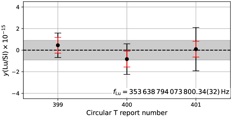
Figure 6: The measured frequency offset for each month (black points) relative to the weighted mean value. Black error bars are the total uncertainties, and red error bars the statistical component only. The weighted mean of all three months is $353\,638\,794\,073\,800.34(32)\,$Hz, with the fractional uncertainty of $9.1\times 10^{-16}$ indicated by the gray shaded region.

5 Discussion

The absolute frequencies obtained for each circular T report are shown in figure 6. The result of $353\,638\,794\,073\,800.34(32)\,$Hz is obtained from the weighted mean of values from the three months. The reduced chi squared is $\chi^{2}_{\nu}=0.56$ with $\nu=2$ degrees of freedom.

The fractional uncertainty of $9.1\times 10^{-16}$ is limited by the satellite link stability and dead time uncertainty. For future campaigns, improved satellite link stability might be achieved by PPP with carrier-phase integer ambiguity resolution (PPP-AR) [32, 33]. Processing of more recent GNSS data with the PPP-AR algorithm implemented by the Natural Resources Canada (NRCan) online service shows an instability of $\sim 1\times 10^{-15}$ at 1 d averaging time, compared to the 5 days observed in this work. To realize this improvement it was also necessary to relocate the rooftop GNSS aerial away from a nearby building partially obstructing the sky. The dead time uncertainty may be reduced by either higher uptime of the optical clock or improved stability of the local frequency reference. A stabilized optical fiber link to the Singapore National Metrology Centre (NMC) has been recently established and will enable linking of our hydrogen masers. An ensemble of hydrogen masers could provide improved stability and better characterisation of the maser noise by continuous observation of the ensemble [34]. With these improvements an absolute frequency measurement at low $10^{-16}$ uncertainty appears feasible. This would be comparable to state-of-the-art measurements based on satellite links to TAI [34, 25, 35] and the accuracy of the caesium primary standards themselves.

References

References

- [1] Weyers S, Gerginov V, Kazda M, Rahm J, Lipphardt B, Dobrev G and Gibble K 2018 Metrologia 55 789
- [2] Beattie S, Jian B, Alcock J, Gertsvolf M, Hendricks R, Szymaniec K and Gibble K 2020 Metrologia 57 035010
- [3] McGrew W, Zhang X, Fasano R, Schäffer S, Beloy K, Nicolodi D, Brown R, Hinkley N, Milani G, Schioppo M et al. 2018 Nature 564 87–90
- [4] Takamoto M, Ushijima I, Ohmae N, Yahagi T, Kokado K, Shinkai H and Katori H 2020 Nat. Photonics 14 411–415
- [5] Sanner C, Huntemann N, Lange R, Tamm C, Peik E, Safronova M S and Porsev S G 2019 Nature 567 204–208
- [6] Aeppli A, Kim K, Warfield W, Safronova M S and Ye J 2024 Phys. Rev. Lett. 133 023401
- [7] Brewer S M, Chen J S, Hankin A M, Clements E R, Chou C w, Wineland D J, Hume D B and Leibrandt D R 2019 Phys. Rev. Lett. 123 033201
- [8] Zhiqiang Z, Arnold K J, Kaewuam R and Barrett M D 2023 Sci. Adv. 9 eadg1971
- [9] Dimarcq N, Gertsvolf M, Mileti G, Bize S, Oates C, Peik E, Calonico D, Ido T, Tavella P, Meynadier F et al. 2024 Metrologia 61 012001
- [10] Barrett M D 2015 New J. Phys. 17 053024
- [11] Kaewuam R, Tan T, Arnold K, Chanu S, Zhang Z and Barrett M 2020 Phys. Rev. Lett. 124 083202
- [12] Arnold K, Jayjong N, Kang M, Qichen Q, Zhang Z, Zhao Q and Barrett M 2024 Phys. Rev. A 110 033115
- [13] Yudin V, Taichenachev A, Oates C, Barber Z, Lemke N, Ludlow A, Sterr U, Lisdat C and Riehle F 2010 Phys. Rev. A 82 011804
- [14] Huntemann N, Lipphardt B, Okhapkin M, Tamm C, Peik E, Taichenachev A and Yudin V 2012 Phys. Rev. Lett. 109 213002
- [15] Sherman J A and Jördens R 2016 Rev. Sci. Instrum. 87 054711
- [16] Petit G and Panfilo G 2018 Optimal traceability to the second through Proc. of 2018 European Frequency and Time Forum (EFTF) pp 185–187
- [17] Jiang Z, Matsakis D and Zhang V 2017 Long-term instability in time links Proc. of the 48th Annual Precise Time and Time Interval Systems and Applications Meeting pp 105–126
- [18] URL https://cddis.nasa.gov/archive/gnss/data/daily/
- [19] Noll C E 2010 Adv. in Space Research 45 1421–1440
- [20] Petit G 2009 The pilot experiment Proc. of 2009 IEEE International Frequency Control Symposium Joint with the 22nd European Frequency and Time forum pp 116–119
- [21] Ray J and Senior K 2005 Metrologia 42 215
- [22] Dach R, Lutz S, Walser P and Fridez P 2015 Bernese GNSS Software Version 5.2 (Astronomical Institute, University of Bern, Bern Open Publishing) ISBN 978-3-906813-05-9
- [23] Zhiqiang Z, Arnold K, Kaewuam R, Safronova M and Barrett M 2020 Phys. Rev. A 102 052834
- [24] Müller J, Dirkx D, Kopeikin S M, Lion G, Panet I, Petit G and Visser P N 2018 Space Science Reviews 214 1–31
- [25] Pizzocaro M, Bregolin F, Barbieri P, Rauf B, Levi F and Calonico D 2020 Metrologia 57 035007
- [26] Yu D H, Weiss M and Parker T E 2007 Metrologia 44 91
- [27] Timmer J and Koenig M 1995 Astronomy and Astrophysics 300 707
- [28] URL https://webtai.bipm.org/ftp/pub/tai/Circular-T/cirt/
- [29] Panfilo G and Parker T E 2010 Metrologia 47 552
- [30] URL https://webtai.bipm.org/ftp/pub/tai/other-products/etoile/
- [31] Hachisu H, Petit G and Ido T 2017 Appl. Phys. B 123 1–5
- [32] Petit G, Meynadier F, Harmegnies A and Parra C 2022 Metrologia 59 045007
- [33] Jian B, Beattie S, Weyers S, Rahm J, Donahue B and Gertsvolf M 2023 Metrologia 60 065002
- [34] Nemitz N, Gotoh T, Nakagawa F, Ito H, Hanado Y, Ido T and Hachisu H 2021 Metrologia 58 025006
- [35] Kim H, Heo M S, Park C Y, Yu D H and Lee W K 2021 Metrologia 58 055007