Scheduling Strategies for Partially-Replicable Task Chains on Two Types of Resources
Working paper version with optimality proof

Abstract

The arrival of heterogeneous (or hybrid) multicore architectures on parallel platforms has brought new performance opportunities for applications and efficiency opportunities to systems. They have also increased the challenges related to thread scheduling, as tasks’ execution times will vary depending if they are placed in big (performance) cores or little (efficient) ones. In this paper, we focus on the challenges heterogeneous multicore problems bring to partially-replicable task chains, such as the ones that implement digital communication standards in Software-Defined Radio (SDR). Our objective is to maximize the throughput of these task chains while also minimizing their power consumption. We model this problem as a pipelined workflow scheduling problem using pipelined and replicated parallelism on two types of resources whose objectives are to minimize the period and to use as many little cores as necessary. We propose two greedy heuristics (FERTAC and 2CATAC) and one optimal dynamic programming (HeRAD) solution to the problem. We evaluate our solutions and compare the quality of their schedules (in period and resource utilization) and their execution times using synthetic task chains and an implementation of the DVB-S2 communication standard running on StreamPU. Our results demonstrate the benefits and drawbacks of the different proposed solutions. On average, FERTAC and 2CATAC achieve near-optimal solutions, with periods that are less than 10% worse than the optimal (HeRAD) using fewer than 2 extra cores. These three scheduling strategies now enable programmers and users of StreamPU to transparently make use of heterogeneous multicore processors and achieve throughputs that differ from their theoretical maximums by less than 8% on average.

I Introduction

Multicore processor architectures composed of different types of cores (also known as heterogeneous, hybrid, or asymmetric) are increasingly common nowadays. What may have started on low power processors with ARM’s big.LITTLE architecture in 2011 [1], has now become present in processors produced by Apple (since 2020), Intel (since 2021) [2], and AMD (since 2023). A common feature in these processors is an ISA shared between the high-performance (or big) and the high-efficiency (or little) cores, which enables the execution of application in both types of cores transparently.

Heterogeneous multicore architectures have multiple advantages, such as providing the opportunity to save energy by turning off big cores when unnecessary (for battery or environmental reasons). They have also been shown to outperform homogeneous architectures under a fixed budget (be it area, power, or both) [3, 4]. We invite the reader to check the survey by Mittal on these processors [5] for more information. These advantages come with the drawback of higher complexity when programming parallel applications for these architectures, as one has to decide how to balance the workload between different cores and core types. When not taking care of their differences, a heterogeneity-oblivious solution can result in lower performance and higher energy consumption (while some cores could be better used).

In this context, we focus on the special characteristics of a kind of parallel application composed of partially-replicable task chains, such as the ones that implement digital communication standards in Software-Defined Radio (SDR) [6]. We consider the problem of scheduling these streaming task chains on two types of resources (heterogeneous multicores) to optimize their throughput and power consumption in a transparent manner, reducing complexity for programmers and end users. Our main contributions in this paper are as follows:

• We provide a formulation of this throughput optimization (period minimization) problem in Section III;

• We propose two greedy heuristics and one optimal dynamic programming solution in Section IV and V;

• We evaluate our new scheduling strategies using simulation, and a real-world digital communication standard (DVB-S2 [7]) by implementing our strategies [8] to work with the StreamPU open source DSEL and runtime system [6] in Section VI.

The remaining sections of this paper are organized as follows: Section II discusses related works, and Section VII provides concluding remarks.

II Related Work

Our main interest lies in the problem of throughput optimization for partially-replicable task chains. We focus on solutions using pipeline and replicated parallelism, and interval mapping [9]. As we are unaware of any solutions to our specific research problem in the state of the art, we will focus our discussion here on variations of this problem.

Throughput on homogeneous architectures: OTAC [10] provides an optimal solution for partially-replicable task chains using pipeline and replicated parallelism. We provide more details about OTAC in Section IV, as our two greedy heuristics are based on its main ideas. OTAC itself is inspired by Nicol’s algorithm [11, 12], which is an optimal solution for the Chain-to-chains partitioning (CCP) problem where only pipelining is possible. Finally, when all tasks are replicable, the optimal solution in homogeneous resources is to build a pipeline with a single stage that is replicated across all resources [13]. Nonetheless, this does not apply for heterogeneous architectures.

Throughput on heterogeneous architectures: Benoit and Robert offered three heuristics for building interval mappings on unrelated heterogeneous architectures [14]. Among them, BSL and BSC use a combination of binary search and greedy allocation, which is similar to the general scheme of OTAC and our proposed heuristics. These heuristics, however, do not consider replicated parallelism.

Makespan on heterogeneous architectures: Topcuoglu et al. [15] introduced HEFT (one of the most used heuristics for this kind of problem) and the CPOP to schedule directed acyclic graphs (DAGs) over unrelated heterogeneous resources. Eyraud-Dubois and Krumar [16] proposed HeteroPrioDep to schedule DAGs over two types of unrelated resources. Sadly, none of these strategies applies for throughput optimization, nor for pipeline and replicated parallelism. Agullo et al. [17] studied the performance of dynamic schedulers on two types of unrelated resources through simulation and real-world experiments. We also employ both kinds of experiments in our evaluation, but dynamic schedulers from current runtime systems are usually inefficient at our task granularity of interest (tens to thousands of $\mu$s) [18]. Benavides et al. [19] proposed a heuristic for the flow shop scheduling problem on unrelated resources, but their solution is not easily transposable for pipeline and replicated parallelism.

SDR on heterogeneous architectures: Mack et al. [20] proposed the use of the CEDR heterogeneous runtime system to encapsulate and enable GNU Radio’s signal processing blocks (tasks) in FPGA and GPU-based systems on chip. They use dynamic scheduling heuristics and imitation learning to co-schedule GNU Radio’s blocks with other applications. In contrast, our approaches build static pipeline decompositions and schedules for a lower runtime overhead. We believe our algorithms can be integrated to GNU Radio in its future version (4.0) [21] when it will abandon its thread-per-block schedule, enabling better performance by avoiding its current issues related to locality and OS scheduling policies [22].

III Problem Definition

The problem of maximizing the throughput of a task chain over two kinds of resources can be modeled as a pipelined workflow scheduling problem [9]. The workflow can be described as a linear chain of $n$ tasks $\mathcal{T}{}=\{\tau_{1},\ldots,\tau_{n}\}$, meaning $\tau_{i}$ can only execute after $\tau_{i-1}$. Tasks are partitioned into two subsets $\mathcal{T}{}_{rep}$ and $\mathcal{T}{}_{seq}$ for replicable (stateless) and sequential (stateful) tasks. Sequential tasks cannot be replicated due to their internal state (i.e., replication leads to false results).

The computing system is composed of two types of unrelated heterogeneous resources $v\in\{\mathcal{B}{},\mathcal{L}{}\}$ representing big and little cores, respectively. Big cores are assumed to have the highest power consumption. The system counts with $b$ big and $l$ little fully-connected cores. Hereafter, the following notation is used to characterize system resources: $R=(b,l)$. A task $\tau_{i}$ has a computation weight (i.e., its latency) $w^{v}_{i}$ that depends on the core type $v$.

The mapping strategy on our system is known as interval mapping [9], where $\mathcal{T}{}$ is partitioned into $k$ contiguous intervals. We call the $i^{th}$ interval in the format $[\tau_{c},\tau_{e}]$ ($c\leq e$) a stage noted as $s_{i}$. A stage is defined as replicable if it contains only replicable tasks. We define $r_{i}$ and $v_{i}$ as the number and the type of resources dedicated to $s_{i}$, respectively. The weight of a stage $s$ with $r$ cores of type $v$ is defined in Eq. (1). Be careful, when $r>1$, the weight of a stage differs from its latency. Other characteristics, such as the communication weights between tasks and network bandwidth are considered out of the scope of our current work due to our focus on heterogeneous multicore architectures (keeping data exchanges local) and interval mapping (which minimizes data transfers).

$$w(s,r,v)=\begin{cases}\sum_{\tau\in s}w^{v}_{\tau}&\text{if}~s\cap\mathcal{T}{}_{seq}\not=\emptyset,~r\geq 1,\\ \frac{1}{r}\sum_{\tau\in s}w^{v}_{\tau}&\text{if}~s\cap\mathcal{T}{}_{seq}=\emptyset,~r\geq 1,\\ \infty&\text{otherwise}\end{cases}$$ (1)

Our main objective is to find a solution $S{}=(\mathsf{s},\mathsf{r},\mathsf{v})$ with $\mathsf{s}=(s_{1},\ldots,s_{k})$ that maximizes throughput. As throughput is inversely proportional to the period, we will refer to this problem as a period minimization problem in the remaining sections. The period of a solution $\mathsf{P}(S{})$ is given by the greatest weight among all stages (Eq. (2)). A solution is only valid if the number of available resources is respected (Eq. (3)).

$$\mathsf{P}(\mathsf{s},\mathsf{r},\mathsf{v})=\max_{i\in[1,k]}w(s_{i},r_{i},v_{i})$$ (2)

$$\sum_{v_{i}=\mathcal{B}{}}r_{i}\leq b,~~~\sum_{v_{i}=\mathcal{L}{}}r_{i}\leq l$$ (3)

Our secondary objective is to minimize the power consumption of the solution (as minimizing energy makes no sense when dealing with a continuous data stream). Solutions to this problem depend on the information available. For instance, if the power consumed by each task in each core type were available (and independent from other tasks in the same core), the objective of period minimization could be prioritized over the power one. A second option would be to assume a fixed power consumption per core used of each type. We chose to work with a different proxy: the use of little cores instead of big ones, as they have lower power consumption. In this case, our secondary objective is to use as many little cores as necessary (and not more) to achieve the minimum period. We will see how this impacts our proposed algorithms in the next sections.

IV New Greedy Heuristics: FERTAC and 2CATAC

We propose two heuristics to schedule partially-replicable task chains on two types of resources. They are both based on OTAC [10] which is able to find optimal solutions for homogeneous resources. In a nutshell, OTAC uses a binary search to set up a target period (similar to Algo. 1) and then tries to greedily build a schedule by packing as many tasks as possible in each stage (as in Algo. 2). Our new heuristics, named FERTAC and 2CATAC, use different means to minimize the period while using as many little cores as necessary. We discuss the main ideas behind them next.

IV-A FERTAC

First Efficient Resources for TAsk Chains, or FERTAC for short, aims to use little cores to build each stage. Big cores are only used when it is not possible to respect the target period. We will explain how FERTAC operates by first covering its methods common to 2CATAC (i.e., Schedule and ComputeStage) and then discussing its specific implementation of the ComputeSolution method (Algo. 4).

Schedule (Algo. 1) follows a binary search procedure similar to the one used for the CCP problem [12]. It sets the lower period bound by the maximum between (I) replicating all tasks over all resources and (II) the sequential task with the largest weight (line 1). The upper period bound is based on the minimum period plus the largest task weight (line 2). The binary search (lines 5–14) tries to find a solution with a target middle period. If the solution is valid, we store it and update the upper bound (lines 9–10), or else we update the lower bound (line 12). The search stops when the difference between the bounds is smaller than an epsilon (line 3) that takes into account the fractional nature of the final period due to replicated stages using multiple cores (Eq. (1)). In total, this requires $O(\log(w_{max}(b+l)))$ calls to ComputeSolution, with $w_{max}=\max_{\tau\in\mathcal{T}}w^{\mathcal{L}{}}_{\tau}$.

Algorithm 1 Schedule (common method)

1:Set of tasks $\mathcal{T}{}$, big cores $b$, little cores $l$.

2:Pipelined and replicated solution $S{}_{best}$.

3:$P_{min}\leftarrow\max(\frac{\sum_{\tau\in\mathcal{T}{}}w^{\mathcal{B}{}}_{\tau}}{b+l},\max_{\tau\in\mathcal{T}{}_{seq}}w^{\mathcal{B}{}}_{\tau})$ $\triangleright$Minimum expected period

4:$P_{max}\leftarrow P_{min}+\max_{\tau\in\mathcal{T}}w^{\mathcal{L}{}}_{\tau}$ $\triangleright$Maximum expected period

5:$\epsilon\leftarrow\frac{1}{b+l}$

6:$S{}_{best}\leftarrow\emptyset$

7:while $P_{max}-P_{min}\geq\epsilon$ do

8: $P_{mid}=\frac{P_{max}+P_{min}}{2}$ $\triangleright$Target period for the binary search iteration

9:$\triangleright$ ComputeSolution is different for FERTAC (Algo. 4) and 2CATAC (Algo. 5)

10: $S{}\leftarrow$ ComputeSolution$(\mathcal{T}{},1,b,l,P_{mid})$

11: if IsValid$(S{},b,l,P_{mid})$ then $\triangleright$Checks for validity (Algo. 3)

12:   $S{}_{best}\leftarrow S{}$ $\triangleright$New best solution

13:   $P_{max}\leftarrow\mathsf{P}(S{})$ $\triangleright$Can only decrease the target period from here

14: else

15:   $P_{min}\leftarrow P_{mid}$ $\triangleright$Can only increase the target period

16: end if

17:end while

18:return $S{}_{best}$

Algorithm 2 ComputeStage (common method)

1:Set of tasks $\mathcal{T}{}$, task index $s$, cores $c$, core type $v$, target period $P$.

2:Task index $e$, used cores $u$.

3:$e\leftarrow$ MaxPacking$(\mathcal{T}{},s,1,v,P)$ $\triangleright$Packs tasks using one core (Algo. 3)

4:$u\leftarrow$ RequiredCores$(\mathcal{T}{},s,e,v,P)$ $\triangleright$Cores needed for this stage (Algo. 3)

5:if $e\neq n$ and IsRep$(\mathcal{T}{},s,e)$ then $\triangleright$If the stage is replicable (Algo. 3)

6: $e\leftarrow$ FinalRepTask$(\mathcal{T}{},s,e)$ $\triangleright$Extends the stage (Algo. 3)

7: $u\leftarrow$ RequiredCores$(\mathcal{T}{},s,e,v,P)$

8: if $u>c$ then $\triangleright$Not enough cores for all tasks, needs to reduce the stage

9:   $e\leftarrow$ MaxPacking$(\mathcal{T}{},s,c,v,P)$ ; $u\leftarrow c$

10: else if $e\neq n$ then $\triangleright$Checks if it is better to leave one core for the next stage

11:   $f\leftarrow$ MaxPacking$(\mathcal{T}{},s,u-1,v,P)$

12:   if RequiredCores$(\mathcal{T}{},f+1,e+1,v,P)=1$ then

13:    $e\leftarrow f$ ; $u\leftarrow u-1$ $\triangleright$Best to reduce the stage

14:   end if

15: end if

16:end if

17:return $e,u$

Algorithm 3 Common support methods

1:IsValid$((\mathsf{s},\mathsf{r},\mathsf{v}),b,l,P):$

2:    return $(|\mathsf{s}|>0$  and $\mathsf{P}(\mathsf{s},\mathsf{r},\mathsf{v})\leq P$  and $\sum_{i\in[1,|\mathsf{v}|]\wedge v_{i}=\mathcal{B}{}}r_{i}\leq b$  and $\sum_{i\in[1,|\mathsf{v}|]\wedge v_{i}=\mathcal{L}{}}r_{i}\leq l)$

3:MaxPacking$(\mathcal{T}{},s,c,v,P):$

4:    return $\max(s,\max_{i\in[s,|\mathcal{T}{}|]}\{i~|~w([\tau_{s},\tau_{i}],c,v)\leq P\})$

5:RequiredCores$(\mathcal{T}{},s,e,v,P):\lceil\frac{w([\tau_{s},\tau_{e}],1,v)}{P}\rceil$

6:IsRep$(\mathcal{T}{},s,e):[\tau_{s},\tau_{e}]\cap\mathcal{T}{}_{seq}=\emptyset$

7:FinalRepTask$(\mathcal{T}{},s,e):\max_{i\in[e,|\mathcal{T}{}|]}\{i~|~$ IsRep$(\mathcal{T}{},s,i)\}$

ComputeStage (Algo. 2) tries to find where to finish a stage and how many cores (of a given type) are required to respect the target period. It first tries to pack as many tasks as possible in the stage using a single core (line 1). We check how many cores the stage requires for the case where the last task in the chain is replicable and its weight surpasses the target period (line 2). If the stage is replicable (line 3), it is extended to include all following replicable tasks (line 4). If this long stage requires more cores than available, it is reduced to respect the target period (lines 5–7). If this stage is not the final one, it means there is a sequential task after it. We check if it is better to move this stage’s final tasks to the next stage while saving one core and, if that is the case, we update the end of the stage (lines 9–12). All these tests guarantee that the stage is packing as many tasks as possible with the given cores.

FERTAC’s ComputeSolution recursively computes a solution for a given target period (Algo. 4) by first trying to build a stage with little cores (line 1), and only moving to big cores if no valid solution was found (lines 2–3). If the stage is final, then it finishes the recursion (lines 8–9). If not, then we are required to continue computing the next stage with the remaining cores (lines 11–13). ComputeSolution returns the list of stages if a valid solution is found (line 15).

Algorithm 4 ComputeSolution for FERTAC

1:Set of tasks $\mathcal{T}{}$, task index $s$, big cores $b$, little cores $l$, target period $P$.

2:Pipelined and replicated [partial] solution.

3:$e,u\leftarrow$ ComputeStage$(\mathcal{T}{},s,l,\mathcal{L}{},P)$ ; $v\leftarrow\mathcal{L}{}$ $\triangleright$Uses little cores (Algo. 2)

4:if not IsValid$(([\tau_{s},\tau_{e}],u,v),b,l,P)$ then $\triangleright$Checks for validity (Algo. 3)

5: $e,u\leftarrow$ ComputeStage$(\mathcal{T}{},s,b,\mathcal{B}{},P)$ ; $v\leftarrow\mathcal{B}{}$ $\triangleright$Needed to use big cores

6: if not IsValid$(([\tau_{s},\tau_{e}],u,v),b,l,P)$ then $\triangleright$No valid solution for both cases

7:   return $(\emptyset,\emptyset,\emptyset)$

8: end if

9:end if

10:if $e=|\mathcal{T}{}|$ then

11: return $([\tau_{s},\tau_{e}],u,v)$ $\triangleright$Returns the valid, final stage

12:else$\triangleright$Needs to continue building stages

13: $b\leftarrow b-u$ if $v=\mathcal{B}{}$ $\triangleright$Updates available cores for next stages

14: $l\leftarrow l-u$ if $v=\mathcal{L}{}$

15: $(\mathsf{s},\mathsf{r},\mathsf{v})\leftarrow$ ComputeSolution$(\mathcal{T}{},e+1,b,l,P)$ $\triangleright$Computes the next stages

16: if IsValid$((\mathsf{s},\mathsf{r},\mathsf{v}),b,l,P)$ then

17:   return $([\tau_{s},\tau_{e}]\cdot\mathsf{s},u\cdot\mathsf{r},v\cdot\mathsf{v})$ $\triangleright$Returns the list of stages

18: else

19:   return $(\emptyset,\emptyset,\emptyset)$

20: end if

21:end if

Regarding the complexity of FERTAC, multiple implementation aspects have to be considered. Given $n=|\mathcal{T}{}|$, we chose to precompute the sum of weights for any given stage using two prefix sums in $O(n)$. We also chose to precompute if any stage is replicable (Algo. 3, line 6) in $O(n^{2})$ for simplicity, but this cost could be amortized by sequentially checking each task (as in OTAC [10]). The validity of a solution (Algo. 3, lines 1–2) has its cost amortized by checking each stage as it is built. Packing tasks in a stage and identifying the final replicable task in a sequence can be done task by task. Finally, it can be seen that each task is considered a constant number of times in ComputeStage (Algo. 2), and a task can only be considered for two stages in sequence (and twice for both types of cores). With all these aspects taken into consideration, our implementation of FERTAC requires $O(n\log(w_{max}(b+l))+n^{2})$ operations.

IV-B 2CATAC

While FERTAC tries to use little cores as soon as possible, Two-Choice Allocation for TAsk Chains (or 2CATAC for short) tries both types of cores for building a stage at each time. This enables the strategy to make better use of little cores in later stages, and to potentially consider different secondary objectives when comparing solutions. This comes at the cost of an exponential increase in the number of solutions to check.

Algorithm 5 ComputeSolution for 2CATAC

1:Set of tasks $\mathcal{T}{}$, task index $s$, big cores $b$, little cores $l$, target period $P$.

2:Pipelined and replicated [partial] solution $S{}_{best}$.

3:for $v\in\{\mathcal{B}{},\mathcal{L}{}\}$ do $\triangleright$Builds solution for this stage with both types of cores

4: $r\leftarrow b$ if $v=\mathcal{B}{}$ else $l$

5: $e_{v},u_{v}\leftarrow$ ComputeStage$(\mathcal{T}{},s,r,v,P)$ $\triangleright$Greedily builds a stage (Algo. 2)

6: if not IsValid$(([\tau_{s},\tau_{e_{v}}],u_{v},v),b,l,P)$ then $\triangleright$Checks for validity (Algo. 3)

7:   $S{}_{v}\leftarrow(\emptyset,\emptyset,\emptyset)$ $\triangleright$No valid stage with this type of cores

8: else if $e_{v}=|\mathcal{T}{}|$ then

9:   $S{}_{v}\leftarrow([\tau_{s},\tau_{e_{v}}],u_{v},v)$ $\triangleright$Valid, final stage option

10: else

11:   $b_{v}\leftarrow b-u_{v}$ if $v=\mathcal{B}{}$ else $b$ $\triangleright$Updates available cores for next stages

12:   $l_{v}\leftarrow l-u_{v}$ if $v=\mathcal{L}{}$ else $l$

13:   $(\mathsf{s}_{v},\mathsf{r}_{v},\mathsf{v}_{v})\leftarrow$ ComputeSolution$(\mathcal{T}{},e_{v}+1,b_{v},l_{v},P)$ $\triangleright$Next stages

14:   if IsValid$((\mathsf{s}_{v},\mathsf{r}_{v},\mathsf{v}_{v}),b_{v},l_{v},P)$ then

15:    $S{}_{v}\leftarrow([\tau_{s},\tau_{e_{v}}]\cdot\mathsf{s}_{v},u_{v}\cdot\mathsf{r}_{v},v\cdot\mathsf{v}_{v})$ $\triangleright$Valid combined solution

16:   else

17:    $S{}_{v}\leftarrow(\emptyset,\emptyset,\emptyset)$

18:   end if

19: end if

20:end for

21:return ChooseBestSolution$(S_{\mathcal{B}}{},S_{\mathcal{L}}{},b,l,P)$ $\triangleright$Picks the best solution (Algo. 6)

Algorithm 6 ChooseBestSolution (part of 2CATAC)

1:Solutions $S_{\mathcal{B}}{}$ and $S_{\mathcal{L}}{}$, big cores $b$, little cores $l$, target period $P$.

2:Pipelined and replicated [partial] solution $S{}_{best}$.

3:if IsValid$(S_{\mathcal{B}}{},b,l,P)$ then $\triangleright$Checks for validity (Algo. 3)

4: if IsValid$(S_{\mathcal{L}}{},b,l,P)$ then

5:   for $v\in\{\mathcal{B}{},\mathcal{L}{}\}$ do $\triangleright$Compares the core usage of the solutions

6:    $(\mathsf{s},\mathsf{r},\mathsf{v})\leftarrow S{}$

7:    $\Sigma b_{v}\leftarrow\sum_{i\in[1,|\mathsf{v}|]\wedge v_{i}=\mathcal{B}{}}r_{i}$

8:    $\Sigma l_{v}\leftarrow\sum_{i\in[1,|\mathsf{v}|]\wedge v_{i}=\mathcal{L}{}}r_{i}$

9:   end for

10:   if $\Sigma l_{\mathcal{B}}{}>\Sigma l_{\mathcal{L}}{}$ and $\Sigma b_{\mathcal{B}}{}<\Sigma b_{\mathcal{L}}{}$ then

11:    $S{}_{best}\leftarrow S_{\mathcal{B}}{}$ $\triangleright$$S_{\mathcal{B}}{}$ makes better usage of little cores

12:   else if $\Sigma l_{\mathcal{B}}{}<\Sigma l_{\mathcal{L}}{}$ and $\Sigma b_{\mathcal{B}}{}>\Sigma b_{\mathcal{L}}{}$ then

13:    $S{}_{best}\leftarrow S_{\mathcal{L}}{}$ $\triangleright$$S_{\mathcal{L}}{}$ makes better usage of little cores

14:   else if $\Sigma l_{\mathcal{B}}{}+\Sigma b_{\mathcal{B}}{}<\Sigma l_{\mathcal{L}}{}+\Sigma b_{\mathcal{L}}{}$ then

15:    $S{}_{best}\leftarrow S_{\mathcal{B}}{}$ $\triangleright$$S_{\mathcal{B}}{}$ uses fewer cores

16:   else

17:    $S{}_{best}\leftarrow S_{\mathcal{L}}{}$ $\triangleright$$S_{\mathcal{L}}{}$ uses fewer cores

18:   end if

19: else

20:   $S{}_{best}\leftarrow S_{\mathcal{B}}{}$ $\triangleright$Only valid solution

21: end if

22:else if IsValid$(S_{\mathcal{L}}{},b,l,P)$ then

23: $S{}_{best}\leftarrow S_{\mathcal{L}}{}$ $\triangleright$Only valid solution

24:else

25: $S{}_{best}\leftarrow(\emptyset,\emptyset,\emptyset)$ $\triangleright$No valid solution

26:end if

27:return $S{}_{best}$

2CATAC’s ComputeSolution (Algo. 5) computes the stage for both big and little cores (lines 1–3). In each case, if the final stage is identified, it is stored for comparison (line 7), or else the recursion is launched for the next stage (line 11) and combined with the current stage (line 13).

ComputeSolution employs ChooseBestSolution (Algo. 6) to compare the solutions for both types of cores. A solution is directly returned if it is the only valid one (lines 18 and 21). In the other case, the solution that better exchanges big cores for little ones is returned (lines 9 and 11) or, in the last scenario, the one that uses fewer cores is chosen (lines 13 and 15). As ComputeSolution’s objective is to find a schedule that respects the target period, there is no need to compare the stages’ weights for the different solutions.

2CATAC’s complexity is defined by its recursion’s possible solutions tree. Other aspects, such as the comparison between two solutions, are amortized by capturing relevant information while computing them. For instance, we provide the accumulated core usages when combining solutions (Algo. 5, line 13) instead of computing them each time (Algo. 6, lines 5–6). Given the considerations previously discussed for FERTAC, we can conclude that 2CATAC displays a worst-case complexity in $O(2^{n}\log(w_{max}(b+l)))$ when each stage contains only one task. This can be prohibitive for larger task chains, but it is still faster than the optimal solution (to be shown next) in some scenarios (see Section VI).

V Optimal Dynamic Programming Solution

Our optimal dynamic programming solution can be defined based on this problem’s recurrence. Let $\mathsf{P}^{*}(j,b,l)$ be the best period achieved when mapping tasks from $\tau_{1}$ to $\tau_{j}$ using up to $b$ big cores and $l$ little cores. $\mathsf{P}^{*}(j,b,l)$ can be computed using the recurrence in Eq. (4) with $\mathsf{P}^{*}(0,b,l)=0$ and $\mathsf{P}^{*}(j,0,0)=\infty$ for $j>0$.

$$\begin{split}\mathsf{P}^{*}(j,b,l)=&\\ \min\limits_{i\in[1,j]}&\begin{cases}\min\limits_{u\in[1,b]}\max\mathsf{P}^{*}(i-1,b-u,l),w([\tau_{i},\tau_{j}],u,\mathcal{B}{})\\ \min\limits_{u\in[1,l]}\max\mathsf{P}^{*}(i-1,b,l-u),w([\tau_{i},\tau_{j}],u,\mathcal{L}{})\end{cases}\end{split}$$ (4)

Eq. (4) shows that an optimal solution can be built from partial optimal solutions. The best solution is found by trying all possible starts for the stage finishing in $\tau_{j}$ and all possible resource distributions between this stage and previous ones for both core types. This recurrence can be computed in $O(j^{2}bl(b+l))$ time and $O(jbl)$ space.

Algorithm 7 HeRAD

1:Set of tasks $\mathcal{T}{}$, big cores $b$, little cores $l$.

2:Pipelined and replicated solution $S{}_{best}$.

3:for $i\in[1,|\mathcal{T}{}|]~,~j\in[0,b]~,~k\in[0,l]$ do $\triangleright$Initializes solution matrix

4: $\mathsf{S}{}_{Pbest}[i][j][k]\leftarrow\infty$ $\triangleright$Minimal maximum period

5: $\mathsf{S}{}_{prev}[i][j][k]\leftarrow(0,0)$ $\triangleright$Big and little cores in the previous stages

6: $\mathsf{S}{}_{acc}[i][j][k]\leftarrow(0,0)$ $\triangleright$Accumulated big and little cores

7: $\mathsf{S}{}_{v}[i][j][k]\leftarrow\mathcal{L}{}$ $\triangleright$Type of core used in the stage

8: $\mathsf{S}{}_{start}[i][j][k]\leftarrow 0$ $\triangleright$Index of the starting task of the stage

9:end for

10:SingleStageSolution$(1,\mathsf{S}{},\mathcal{T}{},b,l)$ $\triangleright$Single task in a single stage (Algo. 8)

11:for $e\in[2,|\mathcal{T}{}|]$ do

12: SingleStageSolution$(e,\mathsf{S}{},\mathcal{T}{},b,l)$ $\triangleright$All $e$ tasks in a single stage (Algo. 8)

13: for $u_{b}\in[0,b]$ do $\triangleright$Solutions with more than one stage

14:   for $u_{l}\in[0,l]$ do $\triangleright$and varying numbers of cores

15:    if $u_{b}\neq 0$ or $u_{l}\neq 0$ then

16:     RecomputeCell$(e,\mathsf{S}{},\mathcal{T}{},u_{b},u_{l})$ $\triangleright$$\mathsf{P}^{*}(e,u_{b},u_{l})$ (Algo. 9)

17:    end if

18:   end for

19: end for

20:end for

21:return ExtractSolution$(\mathsf{S}{},\mathcal{T}{},b,l)$ $\triangleright$Converts the matrix to a solution (Algo. 11)

Algorithm 8 SingleStageSolution (part of HeRAD)

1:Task index $t$, solution matrix $\mathsf{S}{}$, set of tasks $\mathcal{T}{}$, big cores $b$, little cores $l$.

2:Updated $\mathsf{S}{}[t][:][:]$.

3:for $r_{l}\in[1,l]$ do $\triangleright$Initializes row with a stage using little cores

4: $\mathsf{S}{}_{Pbest}[t][0][r_{l}]\leftarrow w([\tau_{1},\tau_{t}],r_{l},\mathcal{L}{})$

5: $\mathsf{S}{}_{acc}[t][0][r_{l}]\leftarrow(0,r_{l})$ if IsRep$(\mathcal{T}{},1,t)$ else $(0,1)$

6:end for

7:for $r_{b}\in[1,b]$ do

8: $w_{b}\leftarrow w([\tau_{1},\tau_{t}],r_{b},\mathcal{B}{})$ $\triangleright$Computes the stage with big cores

9: $u_{b}\leftarrow r_{b}$ if IsRep$(\mathcal{T}{},1,t)$ else $1$

10: for $r_{l}\in[0,l]$ do $\triangleright$Compares if it is better to use $r_{b}$ big

11:   if $w_{b}<\mathsf{S}{}_{Pbest}[t][0][r_{l}]$ then $\triangleright$ or $r_{l}$ little cores for this single stage

12:    $\mathsf{S}{}_{Pbest}[t][r_{b}][r_{l}]\leftarrow w_{b}$

13:    $\mathsf{S}{}_{acc}[t][r_{b}][r_{l}]\leftarrow(u_{b},0)$

14:    $\mathsf{S}{}_{v}[t][r_{b}][r_{l}]\leftarrow\mathcal{B}{}$

15:   else

16:    $\mathsf{S}{}_{Pbest}[t][r_{b}][r_{l}]\leftarrow\mathsf{S}{}_{Pbest}[t][0][r_{l}]$

17:    $\mathsf{S}{}_{acc}[t][r_{b}][r_{l}]\leftarrow\mathsf{S}{}_{acc}[t][0][r_{l}]$

18:   end if

19: end for

20:end for

Algorithm 9 RecomputeCell (part of HeRAD)

1:Task index $j$, solution matrix $\mathsf{S}{}$, set of tasks $\mathcal{T}{}$, big cores available $b$, little cores available $l$.

2:Updated $\mathsf{S}{}[j][b][l]$.

3:$C\leftarrow\mathsf{S}{}[j][b][l]$ $\triangleright$Uses the initial solution from SingleStageSolution (Algo. 8)

4:$C\leftarrow$ CompareCells$(C,\mathsf{S}{}[j][b][l-1])$ if $l>0$ $\triangleright$Compares to neighbor solutions

5:$C\leftarrow$ CompareCells$(C,\mathsf{S}{}[j][b-1][l])$ if $b>0$ $\triangleright$ using one less core

6:for $i\in[1,j]$ in reverse order do $\triangleright$External $\min_{i\in[1,j]}$ (Eq. 4)

7: for $u\in[1,b]$ do $\triangleright$Internal $\min_{u\in[1,b]}$ (Eq. 4)

8:   $B_{Pbest}\leftarrow\max\mathsf{S}{}_{Pbest}[i-1][b-u][l],w([\tau_{i},\tau_{j}],u,\mathcal{B}{})$

9:   $(a_{b},a_{l})\leftarrow\mathsf{S}{}_{acc}[i-1][b-u][l]$

10:   $B_{acc}\leftarrow(a_{b}+u,a_{l})$ if IsRep$(\mathcal{T}{},i,j)$ else $(a_{b}+1,a_{l})$

11:   $B_{prev}\leftarrow(b-u,a_{l})$ ; $B_{v}\leftarrow\mathcal{B}{}$ ; $B_{start}\leftarrow i$

12:   $C\leftarrow$ CompareCells$(C,B)$ $\triangleright$Keeps the best solution (Algo. 10)

13: end for

14: for $u\in[1,l]$ do $\triangleright$Internal $\min_{u\in[1,l]}$ (Eq. 4)

15:   $L_{Pbest}\leftarrow\max\mathsf{S}{}_{Pbest}[i-1][b][l-u],w([\tau_{i},\tau_{j}],u,\mathcal{L}{})$

16:   $(a_{b},a_{l})\leftarrow\mathsf{S}{}_{acc}[i-1][b][l-u]$

17:   $L_{acc}\leftarrow(a_{b},a_{l}+u)$ if IsRep$(\mathcal{T}{},i,j)$ else $(a_{b},a_{l}+1)$

18:   $L_{prev}\leftarrow(a_{b},l-u)$ ; $L_{v}\leftarrow\mathcal{L}{}$ ; $L_{start}\leftarrow i$

19:   $C\leftarrow$ CompareCells$(C,L)$ $\triangleright$Keeps the best solution (Algo. 10)

20: end for

21:end for

22:$\mathsf{S}{}[j][b][l]\leftarrow C$ $\triangleright$Stores the best solution

Algorithm 10 CompareCells (part of HeRAD)

1:Matrix cells for partial solutions $C$ (current) and $N$ (new).

2:Best partial solution.

3:$(c_{b},c_{l})\leftarrow C_{acc}$ ; $(n_{b},n_{l})\leftarrow N_{acc}$

4:if $(C_{Pbest}>N_{Pbest})$  or $(C_{Pbest}=N_{Pbest}$ and $c_{l}<n_{l}$ and $c_{b}>n_{b})$  or $(C_{Pbest}=N_{Pbest}$ and $c_{l}\geq n_{l}$ and $c_{b}\geq n_{b})$ then

5: return $N$

6:else

7: return $C$

8:end if

Algorithm 11 ExtractSolution (part of HeRAD)

1:Solution matrix $\mathsf{S}{}$, set of tasks $\mathcal{T}{}$, big cores $b$, little cores $l$.

2:Pipelined and replicated solution $S{}_{best}$.

3:$e\leftarrow|\mathcal{T}{}|$ ; $s\leftarrow|\mathcal{T}{}|$ ; $r_{b}\leftarrow b$ ; $r_{l}\leftarrow l$

4:$(\mathsf{s},\mathsf{r},\mathsf{v})\leftarrow(\emptyset,\emptyset,\emptyset)$

5:while $e\geq 1$ do

6: $s\leftarrow\mathsf{S}{}_{start}[e][r_{b}][r_{l}]$ $\triangleright$Start of the stage

7: $(u_{b},u_{l})\leftarrow\mathsf{S}{}_{acc}[e][r_{b}][r_{l}]$

8: $v\leftarrow\mathsf{S}{}_{v}[e][r_{b}][r_{l}]$ $\triangleright$Type of core used

9: $(p_{b},p_{l})\leftarrow\mathsf{S}{}_{prev}[e][r_{b}][r_{l}]$

10: if $s>1$ then $\triangleright$Gets the number of cores used in this stage only

11:   $(c_{b},c_{l})\leftarrow\mathsf{S}{}_{acc}[s-1][p_{b}][p_{l}]$

12:   $u_{b}\leftarrow u_{b}-c_{b}$ ; $u_{l}\leftarrow u_{l}-c_{l}$

13: end if

14: $r\leftarrow u_{b}$ if $v=\mathcal{B}{}$ else $u_{l}$ $\triangleright$Number of cores used

15: $(\mathsf{s},\mathsf{r},\mathsf{v})\leftarrow([\tau_{s},\tau_{e}]\cdot\mathsf{s},r\cdot\mathsf{r},v\cdot\mathsf{v})$ $\triangleright$Adds the stage to the solution

16: $e\leftarrow s-1$ ; $r_{b}\leftarrow p_{b}$ ; $r_{l}\leftarrow p_{l}$ $\triangleright$Index for the predecessor stage

17:end while

18:return $(\mathsf{s},\mathsf{r},\mathsf{v})$

HeRAD, or short for Heterogeneous Resource Allocation using Dynamic programming (Algo. 7), implements the optimal strategy of Eq. (4) while also considering the secondary objective of using as many little cores as necessary. It starts by initializing a solution matrix $\mathsf{S}{}$ that will contain all optimal partial solutions (lines 1–7). It then computes all optimal solutions for the first task in the chain with all possible numbers of cores (line 8) using SingleStageSolution. In the next step and for increasing numbers of tasks, the algorithm computes a first solution where all tasks belong to the same stage (line 10). Then, it computes the optimal partial solution for this number of tasks with varying numbers of cores available (line 14) using RecomputeCell. The algorithm finishes by going backwards in the solution matrix and identifying the stages that belong to the optimal solution (line 19) using ExtractSolution (Algo. 11). We have also added an extra step that merges consecutive stages if they are replicable and using the same core type. This has no impact in the minimum period achieved, but it leads to solutions with fewer stages.

SingleStageSolution (Algo. 8) finds the best solutions when putting all considered tasks in the same stage. It computes and stores the weight of the stage using increasing numbers of little cores, taking care to register that sequential stages can only benefit from a single core (lines 1–4). It then considers an increasing number of big cores (lines 6–7) and compares their solutions with the ones using little cores (lines 8–17). It stores the solution with minimum period in the matrix, solving ties in favor of the little cores (lines 9–16).

RecomputeCell (Algo. 9) tries all possible optimal solutions for a scenario with a given number of tasks, big cores and little cores. It uses the solution from SingleStageSolution as a starting point and compares it to other solutions with one fewer big or little core (lines 1–3) that have been previously computed. It then computes all possible solutions for $\max\mathsf{P}^{*}(i-1,b-u,l),w([\tau_{i},\tau_{j}],u,\mathcal{B}{})$ (lines 4–11) and $\max\mathsf{P}^{*}(i-1,b,l-u),w([\tau_{i},\tau_{j}],u,\mathcal{L}{})$ (lines 4 and 12–18), comparing them sequentially to the best solution found so far, and the best solution is stored in the matrix (line 20). We implement an optimization that limits comparisons to a single core (instead of a range of cores in lines 5 and 12) if the stage is sequential. All solution comparisons make use of CompareCells (Algo. 10). It returns the solution with the minimum maximum period. In the case of ties, the solution that better exchanges big cores for little cores is returned or, in the last scenario, the one that uses fewer cores is chosen.

V-A Optimality proof

The optimality of HeRAD can be demonstrated by induction. Its proof combines elements of Eq. (4) and its implementations in Algos. 7, 8, and 9. At each step, we first cover the period minimization aspect of the solution, followed by the idea of using as many little cores as necessary.

Lemma 1.

The solution for $\mathsf{P}^{*}(1,b,l)$ is optimal.

Proof.

The only possible solutions for $\mathsf{P}^{*}(1,b,l)$ include a single pipeline stage using big or little cores. Algo 8 is used to compute the solution for $j=1$ (Algo. 7, line 8). It stores the minimum between the solutions using $b$ big cores or $l$ little cores (Algo 8, lines 5–9), therefore it is optimal in period.

Regarding the use of little cores, the algorithm first computes solutions using them (lines 1–4) and then solves ties with big cores in favor of the little ones (line 9, use of $<$), thus being optimal in this aspect too. ∎

Lemma 2.

The solution for $\mathsf{P}^{*}(j,b,l)$ is optimal if the solutions for $\mathsf{P}^{*}(i,r_{b},r_{l})$ are also optimal for $i<j$, $r_{b}\leq b$, and $r_{l}\leq l$.

Proof.

The period of $\mathsf{P}^{*}(j,b,l)$ takes its value from the minimum period among all possible starts for the stage finishing in $\tau_{j}$ using all possible resource distributions (Eq. (4), loops in Algo. 8 using Algo. 10, and Algo. 9). To consider another schedule with a smaller period is a contradiction, as it requires having a suboptimal $\mathsf{P}^{*}(i,r_{b},r_{l})$, or a value that is smaller than the minimum of all possible solutions, so $\mathsf{P}^{*}(j,b,l)$ is optimal regarding its period.

Regarding the use of little cores, Algo. 10 always solves ties in the benefit of the solution that better exchanges big cores for little cores or the one that uses fewer cores. We also ensure that solutions having one less big or little core available are propagated from previous solutions (Algo. 9 lines 2–3), thus the solution is also optimal in this aspect. ∎

Theorem 1.

HeRAD yields optimal solutions regarding the period achieved and the use of little cores.

Proof.

Lemmas 1 and 2 prove the optimality of the base case and the inductive step, so HeRAD is optimal. ∎

As given by Theorem 1, HeRAD provides schedules with minimal periods while using as many little cores as necessary with the potential issue of a high complexity. We next evaluate how its benefits and drawbacks measure against our greedy heuristics.

VI Experimental Evaluation

Our experimental evaluation is organized in two steps. In the first step, we use synthetic task chains and processors to check how well the strategies are able to optimize our two objectives, and also to profile their execution time. In the second step, we employ them to schedule an implementation of the DVB-S2 digital communication standard [7] on StreamPU [6] and on two heterogeneous multicore processors. Then, we evaluate their throughput. Comparisons include our three strategies and OTAC [10] (which handles homogeneous resources only). We provide more details about our experimental environments and results in the next sections. Source code, result files, and scripts are freely available online [8].

VI-A Experimental Environments

VI-A1 Simulation

Experiments were executed on a Dell Latitude 7420 notebook (Intel Core i7-1185G7 @ 3 GHz, 32 GB LPDDR4 @ 3733 MT/s, 512 GB NVMe SSD) running Linux (Ubuntu 24.04.1 LTS kernel 6.8.0-51, g++ 13.3.0). For period and core usage measurements, 1000 task chains of 20 tasks were generated. Task weights were randomly set in the integer interval [1,100] uniformly for big cores with a slowdown in the interval [1,5] for little cores (rounded using the ceiling function). In order to evaluate how the replicable tasks affect the strategies, the stateless ratio (SR) (i.e., fraction of tasks that are replicable) of each chain was set equal to $\{0.2,0.5,0.8\}$ for different scenarios. We set the number of big ($b$) and little ($l$) cores (e.g., the resources $R=(b,l)$) in the simulation using three different pairs $\{(16_{\mathcal{B}},4_{\mathcal{L}}),(10_{\mathcal{B}},10_{\mathcal{L}}),(4_{\mathcal{B}},16_{\mathcal{L}})\}$. For the execution time profiling, we generate 50 task chains for varying numbers of tasks ($20i|i\in[1,8]$), pairs of numbers of cores ($(20i,20i)|i\in[1,8]$), and SRs.

VI-A2 Real-world SDR Experiment

Experiments were executed on two platforms:

1. an Apple Mac Studio (Apple Silicon M1 Ultra with 20 ARMv8.5-A cores set as 16 (big) p-cores @ 3.2 GHz and 4 (little) e-cores @ 2 GHz, 64 GB LPDDR5 @ 6400 MT/s, 2 TB SSD) running Linux (Fedora 40 Asahi Remix kernel 6.11.8-400, g++ 14.2.1);

2. a Minisforum AtomMan X7 Ti PC (Intel Ultra 9 185H, 16 x86-64 cores with 6 (big) p-cores @ 5.1 GHz, 8 (little) e-cores @ 3.8 GHz, and 2 LPe-cores left unused, 32 GB DDR5 @ 5600 MT/s, 1 TB NVMe SSD) running Linux (Ubuntu 24.10 kernel 6.11.0-13, g++ 14.2.0).

Both run StreamPU v1.6.0 and the open source DVB-S2 transceiver (commit 5a952de). After profiling the DVB-S2 receiver on both platforms (Table III), schedules were computed using all cores and half of them. A compact placement was used for the threads. Each schedule was executed ten times for 1 minute each and the achieved throughputs (in Mb/s and frames per second) were obtained.

VI-B Simulation – Slowdown Compared to HeRAD

Given that HeRAD always provides minimal periods, we use the slowdown ratio $\frac{\mathsf{P}(S{}_{\text{other}})}{\mathsf{P}(S{}_{\text{HeRAD{}}})}$ to compare strategies. Fig. 1(a) illustrates the cumulative distributions (1000 task chains) of slowdown ratios for varying resources and slowdown ratios. Each line represents a strategy, with OTAC (B) (resp. OTAC (L)) using only big (resp. little) cores. We can notice in the first column ($SR=0.2$) that 2CATAC and FERTAC tend to find minimal periods in most cases, but they become less effective as the SR increases (other columns). The higher the SR, the more likely for the period to be limited by replicable tasks and the higher the number of replication options to explore, making it harder to find the best solution.

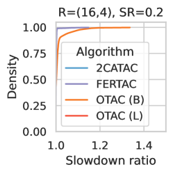
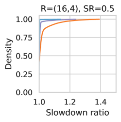
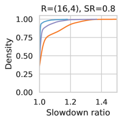
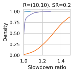
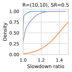
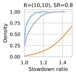
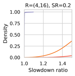
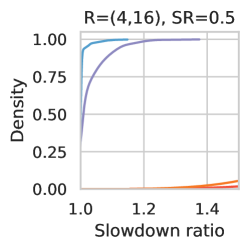
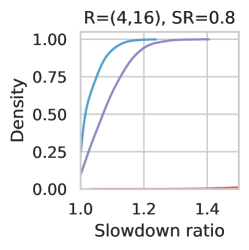
(a) Results zoomed in the slowdown interval $[1,1.5]$. Rows represent different pairs of resources.

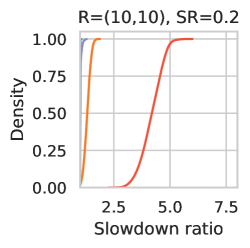
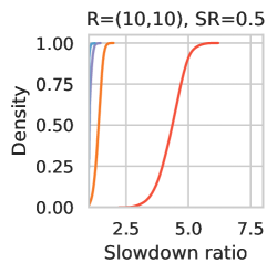
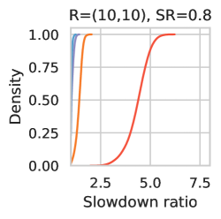
(b) Full slowdown interval for $R=(10_{\mathcal{B}},10_{\mathcal{L}})$.

Figure 1: Cumulative solution (e.g., density) distributions of slowdown ratios (cf. HeRAD) for different heuristics. Columns represent different SRs.

OTAC (B) performs similarly to FERTAC only when many big cores are available (first row). Meanwhile, OTAC (L) never finds optimal solutions because it lacks the big cores to handle the slowest tasks. The gap between these strategies can be better seen in Fig. 1(b) with a full range of slowdown ratios.

We summarize our simulation statistics in Table I. When few little cores are available ($R=(16_{\mathcal{B}},4_{\mathcal{L}})$), 2CATAC and FERTAC find the majority of minimal periods, leading to $1\%$ or lower slowdowns on average. Even for scenarios with different numbers of cores, 2CATAC and FERTAC achieve average slowdown ratios limited to $1.03$ and $1.08$, respectively, which represent $97.1\%$ and $92.6\%$ of the potential throughput. Their worst results ($R=(10_{\mathcal{B}},10_{\mathcal{L}}),SR=0.5$) were limited to maximum slowdowns of $1.23$ and $1.41$, respectively (or $81.3\%$ and $70.1\%$ of the potential throughput). In comparison, OTAC (B) shows average slowdown ratios comparable to the maximum slowdowns of FERTAC for $R=(10_{\mathcal{B}},10_{\mathcal{L}})$, and even worse when even fewer big cores are available. It emphasizes the importance of using both core types together.

TABLE I: Simulation statistics for all scheduling strategies. Each 4-tuple counts the percentage of optimal periods, and the average, median, and maximum slowdown ratios. Each pair indicates the average number of cores used according to their type.

		$SR=0.2$										$SR=0.5$										$SR=0.8$
		Period Statistics						Core Usage				Period Statistics						Core Usage				Period Statistics						Core Usage
$R=(b,l)$	Strategy	(	% opt,	avg,	med,	max	)	(	$b_{\text{used}}$,	$l_{\text{used}}$	)	(	% opt,	avg,	med,	max	)	(	$b_{\text{used}}$,	$l_{\text{used}}$	)	(	% opt,	avg,	med,	max	)	(	$b_{\text{used}}$,	$l_{\text{used}}$	)
$(16_{\mathcal{B}},4_{\mathcal{L}})$	HeRAD	(	100.0%,	1.00,	1.00,	1.00	)	(	11.72,	3.33	)	(	100.0%,	1.00,	1.00,	1.00	)	(	11.97,	3.50	)	(	100.0%,	1.00,	1.00,	1.00	)	(	12.63,	3.49	)
	2CATAC	(	100.0%,	1.00,	1.00,	1.00	)	(	11.74,	3.31	)	(	99.6%,	1.00,	1.00,	1.13	)	(	12.09,	3.47	)	(	93.0%,	1.00,	1.00,	1.17	)	(	12.91,	3.37	)
	FERTAC	(	99.2%,	1.00,	1.00,	1.14	)	(	12.44,	3.91	)	(	95.8%,	1.00,	1.00,	1.22	)	(	12.87,	3.96	)	(	84.3%,	1.01,	1.00,	1.34	)	(	13.30,	3.86	)
	OTAC (B)	(	88.7%,	1.01,	1.00,	1.31	)	(	14.15,	0.00	)	(	82.7%,	1.02,	1.00,	1.35	)	(	14.37,	0.00	)	(	69.9%,	1.04,	1.00,	1.43	)	(	14.41,	0.00	)
	OTAC (L)	(	0.0%,	9.01,	8.93,	13.88	)	(	0.00,	4.00	)	(	0.0%,	9.35,	9.27,	14.81	)	(	0.00,	4.00	)	(	0.0%,	10.57,	10.37,	17.92	)	(	0.00,	4.00	)
$(10_{\mathcal{B}},10_{\mathcal{L}})$	HeRAD	(	100.0%,	1.00,	1.00,	1.00	)	(	9.34,	7.87	)	(	100.0%,	1.00,	1.00,	1.00	)	(	9.02,	9.24	)	(	100.0%,	1.00,	1.00,	1.00	)	(	9.10,	9.44	)
	2CATAC	(	98.8%,	1.00,	1.00,	1.07	)	(	9.34,	7.90	)	(	89.1%,	1.00,	1.00,	1.23	)	(	9.11,	9.28	)	(	61.7%,	1.02,	1.00,	1.22	)	(	9.33,	9.36	)
	FERTAC	(	80.3%,	1.01,	1.00,	1.26	)	(	9.48,	8.87	)	(	51.2%,	1.04,	1.00,	1.41	)	(	9.49,	9.89	)	(	42.2%,	1.06,	1.03,	1.37	)	(	9.56,	9.87	)
	OTAC (B)	(	1.7%,	1.32,	1.32,	1.78	)	(	9.97,	0.00	)	(	1.4%,	1.38,	1.39,	1.87	)	(	9.97,	0.00	)	(	1.6%,	1.41,	1.43,	1.92	)	(	9.99,	0.00	)
	OTAC (L)	(	0.0%,	4.17,	4.19,	5.62	)	(	0.00,	9.57	)	(	0.0%,	4.32,	4.37,	5.80	)	(	0.00,	9.72	)	(	0.0%,	4.34,	4.40,	5.80	)	(	0.00,	9.81	)
$(4_{\mathcal{B}},16_{\mathcal{L}})$	HeRAD	(	100.0%,	1.00,	1.00,	1.00	)	(	3.99,	7.86	)	(	100.0%,	1.00,	1.00,	1.00	)	(	3.99,	13.32	)	(	100.0%,	1.00,	1.00,	1.00	)	(	3.99,	15.80	)
	2CATAC	(	100.0%,	1.00,	1.00,	1.00	)	(	3.99,	7.89	)	(	91.7%,	1.00,	1.00,	1.14	)	(	3.99,	13.42	)	(	41.1%,	1.03,	1.01,	1.21	)	(	3.99,	15.83	)
	FERTAC	(	99.0%,	1.00,	1.00,	1.09	)	(	3.99,	9.27	)	(	61.4%,	1.03,	1.00,	1.34	)	(	3.99,	14.08	)	(	13.0%,	1.08,	1.07,	1.36	)	(	3.99,	15.91	)
	OTAC (B)	(	0.0%,	1.61,	1.59,	2.62	)	(	4.00,	0.00	)	(	0.0%,	2.03,	2.06,	2.88	)	(	4.00,	0.00	)	(	0.0%,	2.42,	2.40,	3.13	)	(	4.00,	0.00	)
	OTAC (L)	(	0.0%,	2.22,	2.16,	4.72	)	(	0.00,	10.98	)	(	0.0%,	2.58,	2.49,	4.72	)	(	0.00,	11.91	)	(	0.0%,	2.57,	2.36,	4.97	)	(	0.00,	13.20	)

Although these results are related to our exact simulation parameters, their general trends are the same for longer task chains or different numbers of resources. Additional experiments (not covered here for the sake of space) have revealed that non-optimal strategies tend to perform worse when more tasks have to be scheduled (more decisions to make), but better when more resources are available (easier to have enough resources for the slowest stage).

VI-C Simulation – Core Usage

Table I also provides the average number of big and little cores used by each scheduling strategy for different resources available and SRs. As our secondary objective is to use as many little cores as necessary to reduce power consumption (Section III), using more little cores and less big ones is desirable. In general, strategies use more cores when more tasks are replicable (right col., $SR=0.8$) to reduce the period.

We can see that 2CATAC tends to use almost the same number of resources as HeRAD. It uses at most $0.3$ more cores than the minimal, sometimes using more big and less little cores. FERTAC, in its part, tends to use more of both resources in its solution. By greedily trying to use little cores in earlier stages, it ends up missing opportunities to make better use of these cores later in the pipeline. Nonetheless, even in its worst average results, FERTAC requires $1.41$ little cores ($R=(4_{\mathcal{B}},16_{\mathcal{L}}),SR=0.2$) or $1.36$ cores in total ($R=(16_{\mathcal{B}},4_{\mathcal{L}}),SR=0.5$) more than HeRAD.

Fig. 2 explores in more detail the differences between FERTAC and HeRAD for one scenario where FERTAC achieved the minimum period $51.2\%$ of the times. Each cell in the heatmaps represent the percentage of times that FERTAC uses more, less, or the same number of big and little cores than HeRAD. When considering all results (Fig. 2(a)), FERTAC uses at most 1 or 2 extra cores $59\%$ and $83.1\%$ of the times, respectively. When considering only the results where FERTAC achieves minimal periods (Fig. 2(b)), the situations where at most 1 or 2 extra cores were necessary change to $21.2\%$ and $39.2\%$ of the times. These differences may be justified given the difference in computational complexity of the strategies, as will be seen next.

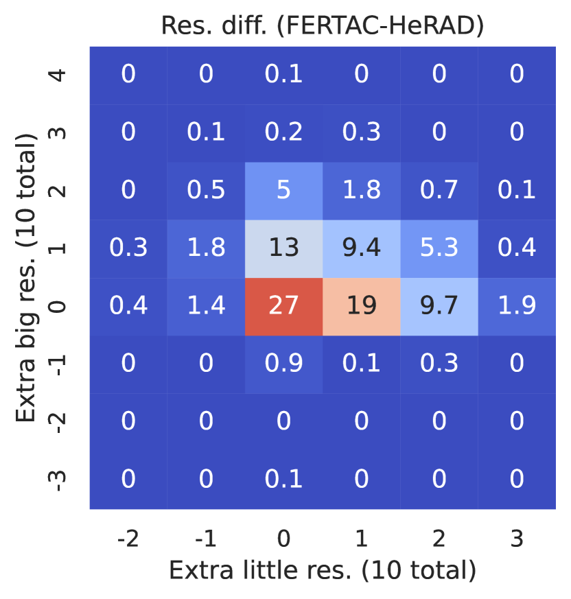
(a) All results.

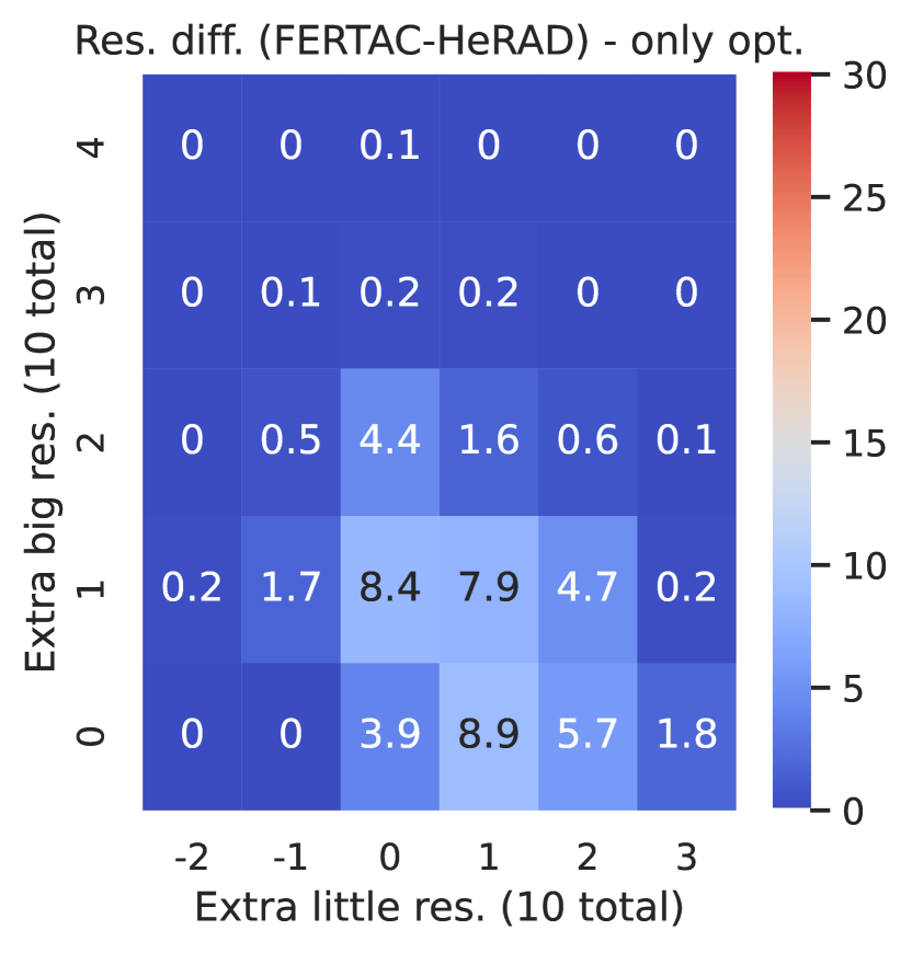
(b) Only optimal periods.

Figure 2: Heatmaps with the differences in resources used between FERTAC and HeRAD for $R=(10_{\mathcal{B}},10_{\mathcal{L}})$ and $SR=0.5$.

VI-D Simulation – Strategies Execution Times

Fig. 3 shows the execution times of the different strategies in $\mu s$ for $R=(20_{\mathcal{B}},20_{\mathcal{L}})$ (Fig. 3(a)) and $R=(100_{\mathcal{B}},100_{\mathcal{L}})$ (Fig. 3(b)). Each point represents the average of 50 runs. Each line represents a strategy computing schedules for task chains with different stateless ratios. The lower the time, the better.

We can notice that FERTAC displays the same behavior as OTAC. Having the lowest computational complexity among proposed strategies, its execution times are in the order of $10$ to $100~\mu s$ and they grow proportionally to the number of tasks.

2CATAC has an exponential complexity in the number of tasks, so its results are limited to up to 60 tasks. Besides its rapid growth in execution time, 2CATAC shows distinct execution times depending on how many replicable tasks there are. Its execution times increase when $SR$ goes from $0.2$ to $0.5$, but then it decreases by almost two orders of magnitude when $SR=0.8$. 2CATAC is able to pack many tasks together in longer pipeline stages when they are replicable, leading to shorter recursions and fewer comparisons. Nonetheless, its exponential behavior limits its usage to short task chains.

HeRAD’s execution times grow with the square of the number of tasks, and they already start in the order of ms in the tested scenarios. Its averages go from $2.476$ ms to $14.381$ ms from 20 to 60 tasks ($R=(20_{\mathcal{B}},20_{\mathcal{L}}),SR=0.8$), and from $78.466$ ms to $3656$ ms ($46.6\times$) from 20 to 160 tasks ($R=(100_{\mathcal{B}},100_{\mathcal{L}}),SR=0.8$). Its execution times are smaller when fewer tasks are replicable due to an optimization in RecomputeCell (see Section V).

Fig. 4 reflects the effects of increasing the number of resources. It shows that the greedy strategies stray mostly unaffected, while HeRAD’s execution times grow. For instance, its execution times go from $1.72~s$ to $6.38~s$ when going from $R=(100_{\mathcal{B}},100_{\mathcal{L}})$ to $R=(160_{\mathcal{B}},160_{\mathcal{L}})$ ($SR=0.8$ in Fig. 4(b)) — a $3.7\times$ increase in time for a $1.6\times$ increase in resources. Although these times are not prohibitive when precomputing a schedule for contemporary task chains and processors, HeRAD could be more difficult to use in bigger scenarios or real-time. We see how its hypothetically optimal schedules behave when applied in a real scenario next.

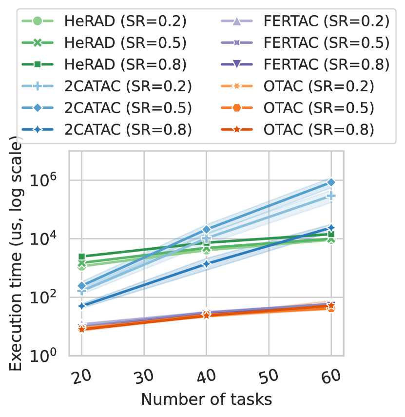
(a) $R=(20_{\mathcal{B}},20_{\mathcal{L}})$.

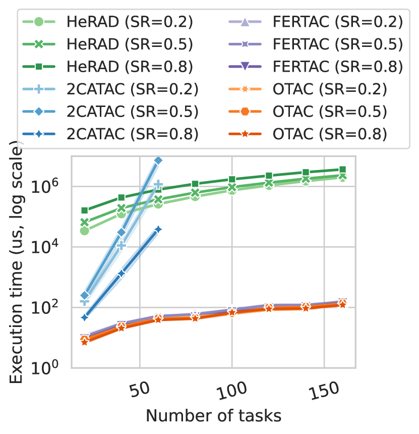
(b) $R=(100_{\mathcal{B}},100_{\mathcal{L}})$.

Figure 3: Average strategy times ($\mu$s, log. scale) with fixed numbers of resources.

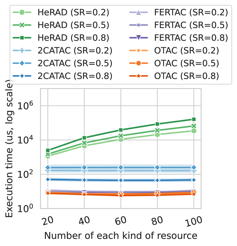
(a) $|\mathcal{T}{}|=20$.

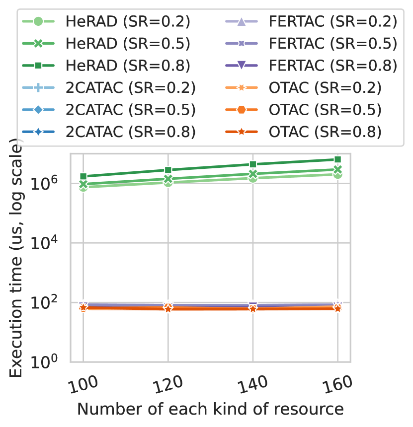
(b) $|\mathcal{T}{}|=100$.

Figure 4: Average strategy times ($\mu$s, log. scale) with fixed numbers of tasks.

VI-E Real-world SDR Experiment – Achieved Throughput

Table II summarizes the solutions found on the different platforms using all or half their cores. They were obtained using the task profiling information listed in Table III. As expected, task latency is always higher on little cores. However, the latency ratio between little and big cores varies according to task and platform. It underlines the need to profile each task independently. In Table II, for each configuration and strategy, the pipeline decomposition is detailed, including the number of little and big cores used, the expected period, and its conversion to throughput metrics. Besides the estimations, the real average FPS and Mb/s values are presented with their absolute and relative differences to the expected values. The information throughput is also illustrated in Fig. 5.

TABLE II: Specification of the configurations $R$ used with the real-world DVB-S2 receiver. Limiting pipeline stages (according to the simulation) are highlighted in orange if replicable, red otherwise.

		Solution							FPS		Info. Throughput (Mb/s)
	$R=(b,l)$	Id	Strategy	Pipeline decomposition where a stage is $(n^{\text{tasks}},r_{v\in\{\mathcal{L},\mathcal{B}\}})$	$|\mathsf{s}|$	$b_{\text{used}}$	$l_{\text{used}}$	Period ($\mu$s)	Sim.	Real	Sim.	Real	Diff.	Ratio
Mac Studio	$(8_{\mathcal{B}},2_{\mathcal{L}})$	$\mathcal{S}_{1}$	HeRAD	$(5,1_{\mathcal{B}}),(1,1_{\mathcal{B}}),(9,1_{\mathcal{B}}),$$(1,2_{\mathcal{B}})$$,(2,1_{\mathcal{L}}),(1,3_{\mathcal{B}}),(4,1_{\mathcal{L}})$	$7$	$8$	$2$	$1128.7$	$3544$	$3316$	$50.4$	$47.2$	$+3.2$	$+7$%
		$\mathcal{S}_{2}$	2CATAC	$(5,1_{\mathcal{B}}),(3,1_{\mathcal{B}}),(7,1_{\mathcal{B}}),$$(4,5_{\mathcal{B}})$$,(4,1_{\mathcal{L}})$	$5$	$8$	$1$	$1154.3$	$3465$	$3590$	$49.3$	$51.1$	$-1.8$	$-4$%
		$\mathcal{S}_{3}$	FERTAC	$(3,1_{\mathcal{L}}),(1,1_{\mathcal{L}}),$$(2,1_{\mathcal{B}})$$,(9,1_{\mathcal{B}}),(5,5_{\mathcal{B}}),(3,1_{\mathcal{B}})$	$6$	$8$	$2$	$1265.6$	$3160$	$2944$	$45.0$	$41.9$	$+3.1$	$+7$%
		$\mathcal{S}_{4}$	OTAC (B)	$(5,1_{\mathcal{B}}),(4,1_{\mathcal{B}}),(6,1_{\mathcal{B}}),$$(4,4_{\mathcal{B}})$$,(4,1_{\mathcal{B}})$	$5$	$8$	$0$	$1442.9$	$2772$	$2677$	$39.5$	$38.1$	$+1.4$	$+4$%
		$\mathcal{S}_{5}$	OTAC (L)	$(16,1_{\mathcal{L}})$$,(7,1_{\mathcal{L}})$	$2$	$0$	$2$	$11440.0$	$350$	$351$	$5.0$	$5.0$	$+0.0$	$+0$%
	$(16_{\mathcal{B}},4_{\mathcal{L}})$	$\mathcal{S}_{6}$	HeRAD	$(3,1_{\mathcal{L}}),(1,1_{\mathcal{L}}),(1,1_{\mathcal{L}}),$$(1,1_{\mathcal{B}})$$,(6,1_{\mathcal{B}}),(7,7_{\mathcal{B}}),(4,1_{\mathcal{L}})$	$7$	$9$	$4$	$950.6$	$4208$	$3934$	$59.9$	$56.0$	$+3.9$	$+7$%
		$\mathcal{S}_{7}$	2CATAC	$(3,1_{\mathcal{L}}),(1,1_{\mathcal{L}}),(1,1_{\mathcal{L}}),$$(1,1_{\mathcal{B}})$$,(9,1_{\mathcal{B}}),(5,7_{\mathcal{B}}),(3,1_{\mathcal{L}})$	$7$	$9$	$4$	$950.6$	$4208$	$3927$	$59.9$	$55.9$	$+4.0$	$+7$%
		$\mathcal{S}_{8}$	FERTAC	$(3,1_{\mathcal{L}}),(1,1_{\mathcal{L}}),(1,1_{\mathcal{L}}),$$(1,1_{\mathcal{B}})$$,(2,1_{\mathcal{L}}),(7,1_{\mathcal{B}}),(5,7_{\mathcal{B}}),(3,1_{\mathcal{B}})$	$8$	$10$	$4$	$950.6$	$4208$	$3920$	$59.9$	$55.8$	$+4.1$	$+7$%
		$\mathcal{S}_{9}$	OTAC (B)	$(5,1_{\mathcal{B}}),$$(1,1_{\mathcal{B}})$$,(9,1_{\mathcal{B}}),(5,7_{\mathcal{B}}),(3,1_{\mathcal{B}})$	$5$	$11$	$0$	$950.6$	$4208$	$3927$	$59.9$	$55.9$	$+4.0$	$+7$%
		$\mathcal{S}_{10}$	OTAC (L)	$(13,1_{\mathcal{L}})$$,(6,2_{\mathcal{L}}),(4,1_{\mathcal{L}})$	$3$	$0$	$4$	$6470.9$	$618$	$611$	$8.8$	$8.7$	$+1.0$	$+1$%
X7 Ti	$(3_{\mathcal{B}},4_{\mathcal{L}})$	$\mathcal{S}_{11}$	HeRAD	$(5,1_{\mathcal{B}}),(10,1_{\mathcal{B}}),(3,1_{\mathcal{B}}),$$(1,3_{\mathcal{L}})$$,(4,1_{\mathcal{L}})$	$5$	$3$	$4$	$2722.1$	$2939$	$2726$	$41.8$	$38.8$	$+3.0$	$+8$%
		$\mathcal{S}_{12}$	2CATAC	$(5,1_{\mathcal{L}}),(10,1_{\mathcal{B}}),(3,1_{\mathcal{B}}),$$(1,3_{\mathcal{L}})$$,(4,1_{\mathcal{B}})$	$5$	$3$	$4$	$2722.1$	$2939$	$2677$	$41.8$	$38.1$	$+3.7$	$+10$%
		$\mathcal{S}_{13}$	FERTAC	$(5,1_{\mathcal{L}}),(3,1_{\mathcal{L}}),(7,1_{\mathcal{L}}),$$(4,3_{\mathcal{B}})$$,(4,1_{\mathcal{L}})$	$5$	$3$	$4$	$2867.0$	$2790$	$2852$	$39.7$	$40.6$	$-0.9$	$-2$%
		$\mathcal{S}_{14}$	OTAC (B)	$(18,1_{\mathcal{B}}),$$(1,1_{\mathcal{B}})$$,(4,1_{\mathcal{B}})$	$3$	$3$	$0$	$6209.0$	$1288$	$1384$	$18.3$	$19.7$	$-1.4$	$-6$%
		$\mathcal{S}_{15}$	OTAC (L)	$(15,1_{\mathcal{L}}),$$(4,2_{\mathcal{L}})$$,(4,1_{\mathcal{L}})$	$3$	$0$	$4$	$7490.3$	$1068$	$1025$	$15.2$	$14.6$	$+0.6$	$+4$%
	$(6_{\mathcal{B}},8_{\mathcal{L}})$	$\mathcal{S}_{16}$	HeRAD	$(5,1_{\mathcal{B}}),$$(1,1_{\mathcal{B}})$$,(6,1_{\mathcal{B}}),(4,2_{\mathcal{B}}),(3,7_{\mathcal{L}}),(4,1_{\mathcal{L}})$	$5$	$6$	$8$	$1341.9$	$5962$	$5108$	$84.8$	$72.5$	$+12.3$	$+17$%
		$\mathcal{S}_{17}$	2CATAC	$(5,1_{\mathcal{B}}),$$(1,1_{\mathcal{B}})$$,(9,1_{\mathcal{B}}),(3,2_{\mathcal{B}}),(2,7_{\mathcal{L}}),(3,1_{\mathcal{L}})$	$5$	$6$	$8$	$1341.9$	$5962$	$5052$	$84.8$	$71.4$	$+13.4$	$+19$%
		$\mathcal{S}_{18}$	FERTAC	$(3,1_{\mathcal{L}}),(2,1_{\mathcal{L}}),(3,1_{\mathcal{B}}),(4,1_{\mathcal{L}}),(6,5_{\mathcal{L}}),$$(1,4_{\mathcal{B}})$$,(4,1_{\mathcal{B}})$	$7$	$6$	$8$	$1552.3$	$5154$	$4602$	$73.3$	$65.4$	$+7.9$	$+12$%
		$\mathcal{S}_{19}$	OTAC (B)	$(8,1_{\mathcal{B}}),(7,1_{\mathcal{B}}),$$(4,3_{\mathcal{B}})$$,(4,1_{\mathcal{B}})$	$4$	$6$	$0$	$2867.0$	$2790$	$2712$	$39.7$	$38.6$	$+1.1$	$+3$%
		$\mathcal{S}_{20}$	OTAC (L)	$(5,1_{\mathcal{L}}),(5,1_{\mathcal{L}}),(5,1_{\mathcal{L}}),$$(4,4_{\mathcal{L}})$$,(4,1_{\mathcal{L}})$	$5$	$0$	$8$	$3745.1$	$2136$	$1833$	$30.4$	$26.1$	$+4.3$	$+16$%

HeRAD, 2CATAC, and FERTAC propose different pipeline decompositions (Table II), which result in different throughputs in practice. We can see in Fig. 5(a) that the strategies achieved similar throughputs when all cores are available ($R=(16_{\mathcal{B}},4_{\mathcal{L}})$). With enough big cores, performance gets limited by a sequential task, leaving many cores unused. On the contrary, performance differs when only half the cores are used ($R=(8_{\mathcal{B}},2_{\mathcal{L}})$). 2CATAC achieves the highest throughput by replicating $5\times$ the stage including the two slowest tasks, while HeRAD separates these tasks in different replicated stages. This leads to a longer pipeline for a $1.02\times$ expected (but not realized) better throughput. FERTAC ends up using both little cores for the first stages, while using a single big core would have been better (see $\mathcal{S}_{1}$ and $\mathcal{S}_{2}$). As so, it lacks the extra core by the end of the pipeline, leading to a lower throughput.

Fig. 5(b) shows a large gap between schedules using half or all cores. HeRAD and 2CATAC require all cores when $R=(6_{\mathcal{B}},8_{\mathcal{L}})$ to get to the point of being limited by a sequential task. Meanwhile, OTAC (B) only gets to $53\%$ of HeRAD’s throughput, which again emphasizes the importance of using both types of cores.

When $R=(6_{\mathcal{B}},8_{\mathcal{L}})$, all solutions from our scheduling strategies ($\mathcal{S}_{[16:18]}$) have two consecutive replicated stages using different types of cores. These required an extension to StreamPU to connect replicated stages. This feature was unavailable before because, when using only homogeneous resources, it is always better to merge consecutive replicated stages [13]. This enhancement has been released in StreamPU v1.6.0. Additionally, we see that this configuration shows the highest differences between expected and obtained throughput results. A common feature of all solutions with differences over $10\%$ is a replicated stage using little cores to handle one of the slowest tasks. We plan to investigate this further to identify if this is related to an architectural characteristic of the processor, to our compact thread placement, to hidden overheads in StreamPU, or some other reason.

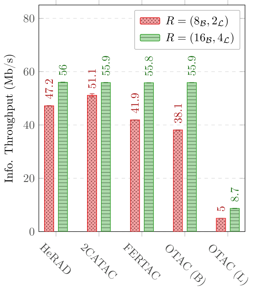
(a) Mac Studio.

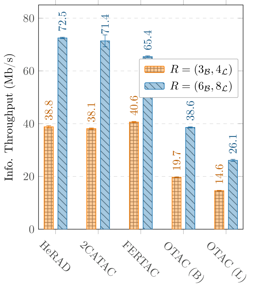
(b) X7 Ti.

Figure 5: Achieved throughput on the DVB-S2 receiver depending on the platform and scheduling strategy.

TABLE III: DVB-S2 receiver’s average task latency on the evaluated platforms. The two slowest sequential and replicable tasks are highlighted in red and orange, respectively.

			Average Latency ($\mu$s)
Task			Mac Studio (4 fra)		X7 Ti (8 fra)
Id	Name	Rep.	$\mathcal{B}$	$\mathcal{L}$	$\mathcal{B}$	$\mathcal{L}$
$\tau_{1}$	Radio – receive	✗	$52.3$	$248.3$	$131.7$	$133.2$
$\tau_{2}$	Multiplier AGC – imultiply	✗	$75.2$	$149.9$	$138.3$	$318.1$
$\tau_{3}$	Sync. Freq. Coarse – synchronize	✗	$96.4$	$496.6$	$113.7$	$429.0$
$\tau_{4}$	Filter Matched – filter (part 1)	✗	$318.9$	$902.9$	$334.8$	$711.9$
$\tau_{5}$	Filter Matched – filter (part 2)	✗	$315.1$	$883.2$	$329.3$	$712.6$
$\tau_{6}$	Sync. Timing – synchronize	✗	$950.6$	$1468.9$	$1341.9$	$2387.1$
$\tau_{7}$	Sync. Timing – extract	✗	$55.5$	$106.0$	$58.7$	$135.1$
$\tau_{8}$	Multiplier AGC – imultiply	✗	$37.1$	$75.4$	$63.5$	$157.4$
$\tau_{9}$	Sync. Frame – synchronize (part 1)	✗	$361.0$	$1064.7$	$365.9$	$848.1$
$\tau_{10}$	Sync. Frame – synchronize (part 2)	✗	$52.9$	$169.1$	$81.1$	$197.9$
$\tau_{11}$	Scrambler Symbol – descramble	✓	$16.0$	$61.0$	$25.1$	$65.9$
$\tau_{12}$	Sync. Freq. Fine L&R – synchronize	✗	$50.5$	$247.1$	$54.3$	$203.2$
$\tau_{13}$	Sync. Freq. Fine P/F – synchronize	✓	$99.2$	$597.8$	$253.8$	$356.2$
$\tau_{14}$	Framer PLH – remove	✓	$23.4$	$65.1$	$47.4$	$87.7$
$\tau_{15}$	Noise Estimator – estimate	✓	$40.5$	$65.4$	$32.4$	$65.4$
$\tau_{16}$	Modem QPSK – demodulate	✓	$2257.5$	$4838.6$	$2123.1$	$5742.4$
$\tau_{17}$	Interleaver – deinterleave	✓	$21.1$	$58.4$	$29.3$	$47.6$
$\tau_{18}$	Decoder LDPC – decode SIHO	✓	$153.2$	$506.7$	$239.7$	$1024.4$
$\tau_{19}$	Decoder BCH – decode HIHO	✓	$3339.9$	$7303.5$	$6209.0$	$8166.2$
$\tau_{20}$	Scrambler Binary – descramble	✓	$191.7$	$464.9$	$559.0$	$621.8$
$\tau_{21}$	Sink Binary File – send	✗	$9.5$	$33.3$	$34.6$	$75.6$
$\tau_{22}$	Source – generate	✗	$4.0$	$13.6$	$16.9$	$23.4$
$\tau_{23}$	Monitor – check errors	✓	$9.5$	$21.0$	$9.2$	$20.5$
Total			$8530.8$	$19841.3$	$12592.5$	$22530.7$

A final point to notice in Fig. 5(b) and Table II is that FERTAC obtains the best throughput for $R=(3_{\mathcal{B}},4_{\mathcal{L}})$. Although its expected throughput is only $95\%$ of the optimal, it achieved a throughput $4.5\%$ higher than HeRAD. The main difference in its solution is the use of big cores to replicate the stage with the two slowest tasks, which led to a result better than expected. This insight points to possible practical improvements to our scheduling solutions in the future.

VII Concluding Remarks

In this paper, we considered the problem of scheduling partially-replicable task chains on two types of resources to optimize throughput (minimize period) and power consumption (use as many little cores as necessary). We have proposed two greedy strategies (FERTAC that tries to use little cores as early as possible, and 2CATAC that tries to use both core types at each stage) and one optimal dynamic programming strategy (HeRAD). Fig. 6 summarizes their main characteristics based on our experimental evaluation and analysis.

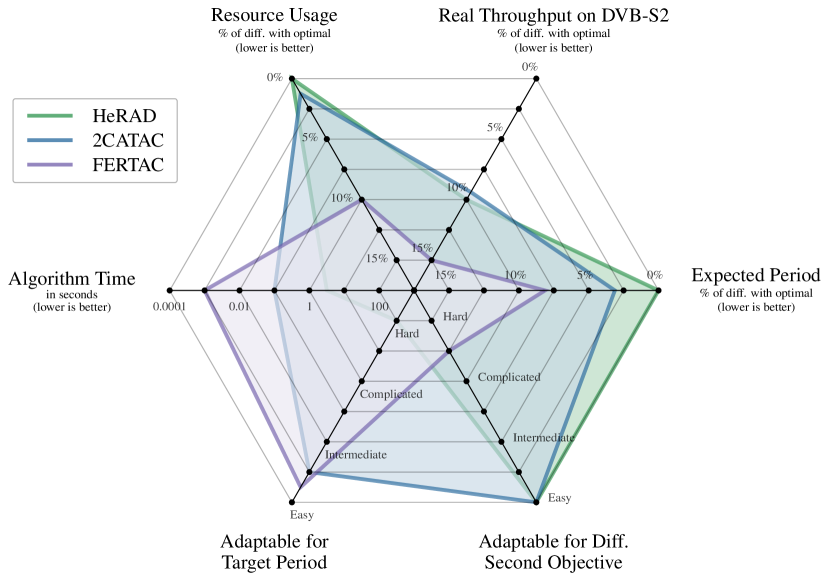
Figure 6: Advantages and limitations of the proposed strategies.

Using simulation, we have verified that FERTAC and 2CATAC are able to obtain near-optimal schedules on average, with minor increases in period and resource utilization. We have shown that the general quality of their schedules is affected by characteristics of the platform (number of cores) and the task chain (e.g., the number of replicable tasks).

Our real-world experiments with the DVB-S2 receiver task chain in two heterogeneous multicore platforms have enabled us to validate our scheduling strategies, with each algorithm achieving the highest throughput in at least one configuration. Fig. 6 shows that, on average, the real throughput difference compared to the best theoretical throughput (from HeRAD’s expected period) ranges between 9% for 2CATAC and 15% for FERTAC, considering that HeRAD itself achieves 10% differences of its target. We think this as a positive result when moving from theory to practice. Our results have also emphasized the importance of using both types of cores, as the optimal solution for homogeneous resources (OTAC) usually lagged behind our scheduling strategies.

As future work, we intend to take lessons from our experimental evaluation to improve future solutions. We will profile the communication and synchronization overheads on StreamPU to understand how they affect the schedules and include them in our model, if necessary. We will study how to incorporate some of the features of our best schedules (such as shorter pipelines) into our strategies, and also how to use direct power measurements instead of assumptions about the architectures to optimize energy consumption. Additionally, we plan to evaluate the impact on placing multiple stages on the same core to benefit from simultaneous multithreading and very low communication overhead. Finally, we would like to evaluate the impact of thread placement on the achieved throughput and on the energy consumption.

References

- [1] R. Randhawa, “Software techniques for ARM big.LITTLE systems,” 2013.
- [2] E. Rotem et al., “Intel Alder Lake CPU architectures,” IEEE Micro, vol. 42, no. 3, pp. 13–19, 2022.
- [3] R. Kumar et al., “Single-ISA heterogeneous multi-core architectures: The potential for processor power reduction,” in International Symposium on Microarchitecture. IEEE, 2003.
- [4] R. Rodrigues et al., “Performance per Watt benefits of dynamic core morphing in asymmetric multicores,” in International Conference on Parallel Architectures and Compilation Techniques. IEEE, 2011.
- [5] S. Mittal, “A survey of techniques for architecting and managing asymmetric multicore processors,” ACM Computing Surveys, vol. 48, no. 3, pp. 1–38, 2016.
- [6] A. Cassagne et al., “StreamPU: A DSEL for high throughput and low latency software-defined radio on multicore CPUs,” Wiley Conc. and Comput.: Practice and Experience, vol. 35, no. 23, p. e7820, 2023.
- [7] ETSI EN 302 307 V1.2.1, “Digital Video Broadcasting (DVB); Second generation framing structure, channel coding and modulation systems for Broadcasting, Interactive Services, News Gathering and other broadband satellite applications (DVB-S2),” 2009.
- [8] L. Lima Pilla, “AMP scheduling source code repository,” tag v1.0, Commit 9ee0279 – 2025-02-06. [Online]. Available: https://github.com/aff3ct/amp-scheduling/
- [9] A. Benoit, U. V. Çatalyürek, Y. Robert, and E. Saule, “A survey of pipelined workflow scheduling: Models and algorithms,” ACM Computing Surveys, vol. 45, no. 4, 2013.
- [10] D. Orhan et al., “OTAC: Optimal scheduling for pipelined and replicated task chains for software-defined radio,” Oct. 2023, working paper or preprint. [Online]. Available: https://hal.science/hal-04228117
- [11] D. Nicol, “Rectilinear partitioning of irregular data parallel computations,” Elsevier Journal of Parallel and Distributed Computing, vol. 23, no. 2, pp. 119–134, 1994.
- [12] A. Pınar and C. Aykanat, “Fast optimal load balancing algorithms for 1D partitioning,” Elsevier Journal of Parallel and Distributed Computing, vol. 64, no. 8, pp. 974–996, 2004.
- [13] A. Benoit and Y. Robert, “Complexity results for throughput and latency optimization of replicated and data-parallel workflows,” Springer Algorithmica, vol. 57, no. 4, pp. 689–724, 2010.
- [14] ——, “Mapping pipeline skeletons onto heterogeneous platforms,” Elsevier Journal of Parallel and Distributed Computing, vol. 68, no. 6, pp. 790–808, 2008.
- [15] H. Topcuoglu, S. Hariri, and M.-Y. Wu, “Task scheduling algorithms for heterogeneous processors,” in Heterogeneous Computing Workshop. IEEE, 1999.
- [16] L. Eyraud-Dubois and S. Kumar, “Analysis of a list scheduling algorithm for task graphs on two types of resources,” in International Parallel and Distributed Processing Symposium. IEEE, 2020.
- [17] E. Agullo et al., “Bridging the gap between performance and bounds of Cholesky factorization on heterogeneous platforms,” in International Parallel and Distributed Processing Symposium Workshop. IEEE, 2015.
- [18] E. Slaughter et al., “Task bench: A parameterized benchmark for evaluating parallel runtime performance,” in Super Computing. ACM, 2020.
- [19] A. J. Benavides, M. Ritt, and C. Miralles, “Flow shop scheduling with heterogeneous workers,” Elsevier European Journal of Operational Research, vol. 237, no. 2, pp. 713–720, 2014.
- [20] J. Mack, S. Gener, A. Akoglu, J. Holtom, A. Chiriyath, C. Chakrabarti, D. Bliss, A. Krishnakumar, A. Goksoy, and U. Ogras, “GNU Radio and CEDR: Runtime scheduling to heterogeneous accelerators,” in GRCon. GNU Radio Foundation, 2022.
- [21] J. Morman, M. Lichtman, and M. Müller, “The future of GNU Radio: Heterogeneous computing, distributed processing, and scheduler-as-a-plugin,” in Military Communications Conference. IEEE, 2022.
- [22] B. Bloessl, M. Müller, and M. Hollick, “Benchmarking and profiling the GNU Radio schedulers,” in GRCon. GNU Radio Foundation, 2019.
- [23] K. Agrawal, A. Benoit, and Y. Robert, “Mapping linear workflows with computation/communication overlap,” in International Conference on Parallel and Distributed Systems. IEEE, 2008.
- [24] A. L. Nunes et al., “Optimal time and energy-aware client selection algorithms for federated learning on heterogeneous resources,” in International Symposium on Computer Architecture and High Performance Computing. IEEE, 2024.