Edge detection with polynomial frames on the sphere
Abstract
In a recent article, we have shown that a variety of localized polynomial frames, including isotropic as well as directional systems, are suitable for detecting jump discontinuities along circles on the sphere. More precisely, such edges can be identified in terms of their position and orientation by the asymptotic decay of the frame coefficients in an arbitrary small neighborhood. In this paper, we will extend these results to discontinuities which lie along general smooth curves. In particular, we prove upper and lower estimates for the frame coefficients when the analysis function is concentrated in the vicinity of such a singularity. The estimates are given in an asymptotic sense, with respect to some dilation parameter, and they hold uniformly in a neighborhood of the smooth curve segment under consideration.
Keywords.
Detection of singularities, analysis of edges, wavelets on the sphere, polynomial frames, directional wavelets.
Mathematics Subject Classification.
42C15, 42C40, 65T60
1 Introduction
The classical orthonormal basis of spherical harmonics plays a fundamental role in signal analysis on the sphere . It allows for a unique representation
of any signal with respect to this basis and is completely determined by its Fourier coefficients . However, in general it is not obvious how one can extract some desired information about from these inner products. Here, the study of localized features proves to be particularly difficult, since the spherical harmonics are not concentrated in space and, thus, the coefficients are global quantities. One way to tackle this problem is to consider frames consisting of localized functions. Indeed, if is such a system, the frame coefficients , which, again, contain all the information about the signal , give access to a position-based analysis. Furthermore, if the are polynomials, then the inner products can be computed as linear combinations of the Fourier coefficients . In this paper, we prove that, for a wide class of localized polynomial frames on the sphere, the frame coefficients display accurately the positions and orientations of jump discontinuities which lie along sufficiently smooth curves.
In the one-dimensional setting, the problem of detecting singularities with localized polynomial frames has been well investigated (see e.g. [5, 10, 11, 12]). As a more recent development, the bivariate case has also received a lot of attention (see e.g. [2, 3, 6, 16, 17]). Here, the problem is more complex since singularities can lie along curves and, consequently, directional frames are needed to identify such features both in terms of their position and orientation. On the sphere , this matter was first investigated in the previous article [18], where the results are limited to singularities on circles. In this present paper, we will investigate the detection of jump discontinuities that lie along more general curves. Our approach is based on the study of frame coefficients with respect to indicator functions , where is a simply connected region with a sufficiently smooth boundary . Here, we take advantage of the fact that, locally, smooth curves are approximated sufficiently well by suitable circles. This allows us to transfer some of our previous results to this more general setting. Specifically, for the class of directional wavelets , introduced and studied in [7, 8, 19], we show that the frame coefficients peak when the distance between the center of the rotated wavelet and the boundary is small enough and exhibits roughly the same orientation as the closest edge segment. Indeed, in Theorem 4.3 we will show that there exists some and a nonempty open interval such that
provided that the orientation does not deviate too much from the orientation of the nearest edge. Here, larger values of the dilation parameter result in a better localization of the corresponding wavelet. Additionally, we derive an upper bound of the form
where is some positive integer. The constants can be chosen independent of and , as long as the wavelet is positioned in some neighborhood of the curve segment under consideration. Another insightful result about the frame coefficients will be presented in Theorem 4.4, consisting of an asymptotic formula in which the leading term is given explicitly as function depending essentially on the difference in position and orientation between the wavelet and the closest boundary segment. Even though all our findings are formulated in terms of the continuous wavelet transform, the implications for corresponding discretized systems, as discussed for example in [8, 19], are obvious.
The remainder of this paper is organized as follows. In Section 2, we go over some basic notations and give an explicit basis of spherical harmonics. Section 3 serves as a short introduction to the system of directional wavelets [7, 8, 19]. Furthermore, we formulate a new localization bound which has a simple proof and slightly improves the bound given in [7]. In Section 4, we present our main results, which are derived in two primary steps. First, we prove an auxiliary lemma which states that, locally, smooth curves are approximated sufficiently well by suitable circles. Subsequently, we combine said lemma with our previous results in [18] to obtain the desired asymptotic estimates. Finally, in Section 5, we present some numerical experiments which illustrate our theoretical findings.
2 Preliminaries
We consider the space equipped with the euclidean norm , which is induced by the inner product for . The vectors
form the canonical basis of . As usual, we will denote the two-dimensional unit sphere by and refer to as the north pole of . Each point can be identified in terms of its latitude and, not necessarily unique, longitude through
| (1) |
The geodesic distance between two points is given by
It is well known that is a metric on and that
| (2) |
The set
is called a spherical cap with center and opening angle . Its boundary
constitutes a circle on the sphere. Furthermore, in the case that , we call a great circle. Finally, if and we define
In the following, we consider the Hilbert space of square integrable functions on with the corresponding inner product
where is the usual surface element. A common choice for a polynomial orthonormal basis consists of the functions , where denotes the spherical harmonic of degree and order defined as
| (3) |
The associated Legendre polynomials used in (3) are given by
| (4) |
and
where the Legendre polynomial can be defined via the Rodrigues formula
If is a continuous function defined on the sphere, we use the standard notation
Functions in can be rotated using elements in the rotation group . In this paper, we will often refer to a parameterization of rotation matrices in terms of elements in the unit tangent bundle , where denotes the tangent space of at . Here, the correspondence is given by the bijection ,
Hence, is the unique rotation matrix mapping to and to . In this context, we define the rotation operator by
| (5) |
In the literature, elements of the rotation group are also commonly represented as matrices in terms of the Euler angles and , where and is the rotation matrix which rotates around the -axis by an angle . The rotation operator can then also be given in terms of and through
While for the most part we will use the unit tangent bundle parameterization of , occasionally we will also refer to the Euler angle representation. A connection between these two approaches is given by
with and .
Finally, for we define to be the order dependent angle between two vectors , i.e., , where is the matrix performing a counterclockwise rotation around the axis by the angle .
3 Localized polynomial frames on the sphere
In the series of papers [7, 8, 19] the authors introduced and investigated systems of so called directional wavelets on the sphere, which constitute a wide class of isotropic and non-isotropic polynomial frames. These frame functions are highly localized in space and therefore provide a powerful tool for position-based analyses. Following closely the construction and notation in [7], we define the directional wavelets in terms of their Fourier coefficients by
| (6) |
where is a window function satisfying for some and . The spatial localization of is controlled by the dilation parameter , where larger values correspond to higher concentrated wavelet functions. As suggested in [7], for we define the directionality component by
where
and
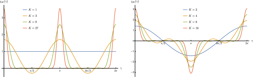
This results in for , i.e., the directional wavelets are band-limited with respect to the azimuthal frequency. Furthermore, becomes increasingly more directional as gets large. Since does not depend on for , we will also write instead of in this case. We will see that the function
which is essentially the inverse Fourier transform of the directionality component, characterizes the directional sensitivity of with respect to detecting discontinuities. Indeed, in the special case where the singularities lie along circles this was previously observed in [18, Theorem 3.1]. The functions are visualized in Figure 1 for different values of .
The localization bound for directional wavelets derived in [7] plays a central role in the proof of our main results. Therefore, we would like to reproduce the corresponding statement here once again, using our slightly different notation. Moreover, we give an alternative simple proof, which is based on [1, Theorem 2.6.7], and our result improves the existing bound stated in [7]. Here, and in the remainder of the article, all occurring constants only depend on the indicated parameters and their values might change with each appearance.
Proposition 3.1.
Let be the directional wavelet defined in (6) with for some . Then there exists a constant such that
| (7) |
In particular,
| (8) |
Proof.
For , the occurring directionality components in (6) are independent of , i.e., . By using the symmetry , as well as (3) and (4), we obtain
where
In the following, we will fix and derive an upper bound for the above inner sum. For any there are constants such that
Thus, we have
where
The classical Markov-inequality for algebraic polynomials yields
and consequently . It will be sufficient to choose . Additionally,
with and . Now, we can apply [1, Theorem 2.6.7] and obtain
This completes the proof of the estimate (7). The inequality in (8) is now a simple consequence. Indeed, by (7) it suffices to show that
This, however, is obvious in both cases , where we have , and , where . ∎
If , the corresponding wavelets
| (9) |
are isotropic and they can be interpreted as univariate polynomials on the interval . Such systems are characterized by their simple structure and have been well investigated in the literature (see e.g. [1, 9, 12, 13, 14, 15]). In this case, the upper bound (8) can be derived under less strict smoothness conditions on the window function . A proof of this fact can be found in [15, Theorem 1]. In our notation, this statement reads as follows.
Proposition 3.2.
Let be the directional wavelet defined in (9) with for some and . Then there exists some constant such that
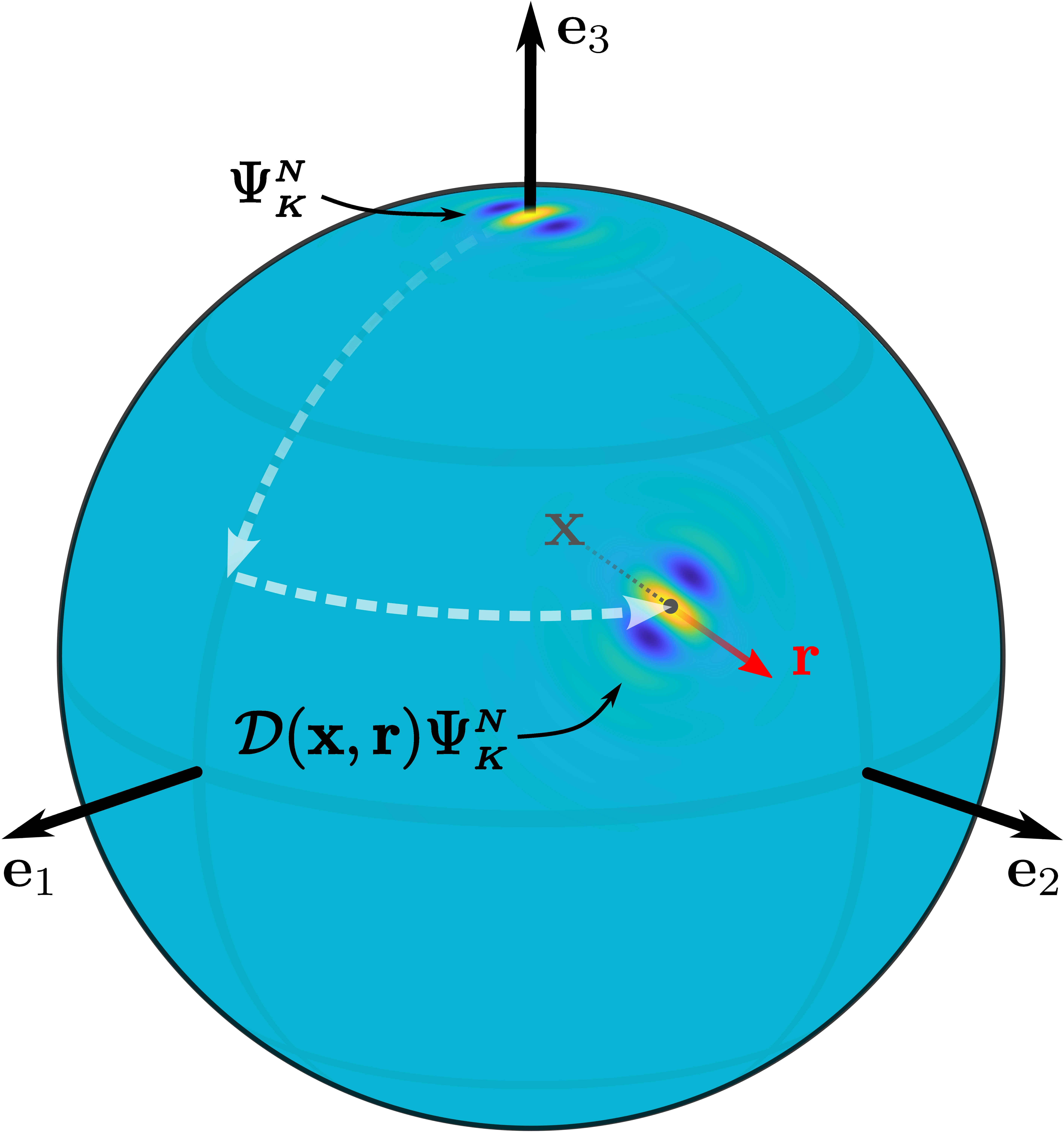
In summary, the directional wavelets defined in (6) are localized at the north pole and get more and more concentrated as the dilation parameter increases. The directional sensitivity of is determined by , where larger values correspond to wavelets with a higher directionality. Furthermore, motivated by Figure 2, we will say that points in the direction .
In the series of papers [7, 8, 19] the authors discussed how one can construct frames by considering rotated versions of the and adding a suitable scaling function. In this article, the concept of rotated wavelets also plays a central role and the operator defined in (5) has an easy interpretation. Indeed, as visualized in Figure 2, the function is localized at and points in the direction .
4 Edge detection
We begin by describing the situation to which we will refer throughout this section. Let be a set whose boundary is the image of a closed unit-speed curve
of finite length , where is injective except for . We assume that there exists an interval , , such that . Also, we will assume that has a positive orientation, such that for each we have
provided that is small enough. For , the curvature of at will play an important part in our calculations. It holds that , which can be verified as follows. Since is a unit speed curve on the sphere, we have for all . Thus, differentiating twice on both sides, we obtain . Consequently, the Cauchy-Schwarz inequality yields . We now define
Obviously, . In the following, we will assume that
| (10) |
for all . The latter can of course always be satisfied by choosing the interval small enough. If is sufficiently small, we write and define
| (11) |
Note that since the continuous map attains its minimum on the compact set and this value must be greater than zero due to the injectivity of . From now on we assume to be fixed. Our results will be stated in the form of asymptotic estimates for the inner products which hold uniformly for all with
| (12) |
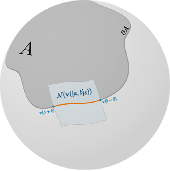
As illustrated in Figure 3, the set of all points satisfying (12) constitutes a certain neighborhood of the curve segment and will be denoted by . In particular, we point out that for each there exists a unique such that
| (13) |
Indeed, the existence of such a point is obvious. To verify the uniqueness, let us assume that and are two different points in with . Then, the spherical cap which is centered at and has the opening angle , the upper bound following from the condition in (12), clearly does not contain any point of since we defined spherical caps to be open sets. Consequently, as the boundary of the mentioned cap has a curvature of at least , there must exist a point between and such that . This, however, contradicts the definition of . In the following, when is given, we will always use the symbol to refer to the unique point in satisfying (13).
4.1 A key lemma
Before presenting our main results, we will prove the following auxiliary lemma, which gives an upper bound on some approximation error when representing the smooth curve segment locally by circles. This will enable us to reduce the problem of detecting jump discontinuities along -curves to estimating the frame coefficients of indicator functions of spherical caps. We note that a similar approach was taken in [2] for the Euclidean setting.
Lemma 4.1.
Let . Then there exists a unique spherical cap whose boundary has an arc-length parameterization
i.e., the length of equals , such that
-
1.
, , and
-
2.
for each there exists some with and , i.e., the boundary curve is positively oriented.
Furthermore, if and is the corresponding point with , then
| (14) |
Here, is a global constant which does not depend on any of the parameters. In particular, the upper bound does not depend on the choice of .
In the proof of this lemma, we will make use of the following relation between the distance of two points with equal latitude and the difference of their longitudinal coordinates.
Lemma 4.2.
Let and . Then
In particular, for , is an even function which is strictly increasing on and
Proof.
Since the first statement is trivial for , we can assume that . Using (1), the equality
follows by a straightforward calculation. Additionally, the inequality yields
Finally, by applying , we obtain the desired inequality. ∎
Proof of Lemma 4.1.
Let . Since the curvature of at must be at least , we can choose such that . Without loss of generality, let
It then follows that either
Indeed, differentiating both sides of yields . Similarly, by differentiating both sides of twice, we see that . Thus, if , , we have
and consequently or . Since rotating the whole setup by transfers to , switches the sign of and keeps invariant, we can assume that . Now, if , then
| (15) |
defines a unit speed curve with , and , as one can easily verify. For , choose the inverted curve . Indeed, the image of yields the unique circle on the sphere which has a parameterization satisfying these properties. Furthermore, there are exactly two spherical caps whose boundary is equal to the image of , only one of which, we will call it , satisfying the second condition stated in Lemma 4.1. This completes the first part of the proof.
Now, let and with . Also, let such that . Just like in the first part of the proof, we can assume that , and . Moreover, we only consider the case as otherwise the proof is completely analogous. In the following, we will use the notation
| (16) |
which is justified by (1). Clearly, and . Additionally, (10) implies that for each we have
and therefore
| (17) |
as well as
| (18) |
Using (17), an elementary calculation yields
According to (16), we have
Since is a function in , we conclude that . Furthermore,
| (19) |
Here,
| (20) |
which can be verified as follows. Using (17) and (18), together with the fact that , we first obtain
Additionally, by (18), it holds that
which confirms (20). Therefore, together with
we obtain
| (21) |
In particular, is strictly increasing on and thus the inverse function , where
exists. Of course, is continuous. Additionally, with
Consequently, the mean value theorem yields
| (22) |
After these preliminary considerations, we can now approximate locally, meaning at the point , by the boundary of a suitable spherical cap. Note that by Taylor’s theorem we have
| (23) |
for each , where lies between and and
We will now consider the unique spherical cap given in the first part of the proof. Locally, its boundary corresponds to the curve
This re-parameterization of (15) allows us express the boundary locally in such a way that the longitudinal coordinates of and are equal for all . Using (19), it is straightforward to show that , as well as
Consequently, Taylor’s theorem yields
| (24) |
for , where lies between and . Additionally, elementary calculations yield
Thus, combining (23) and (24), we obtain
| (25) |
Finally, let us prove the estimate (14). Under the given assumptions, does not contain any points with . Indeed, if such a point would exist, then . But since has the minimal distance towards among all points of , we conclude that and therefore . However, this contradicts the definition of .
Next, we show that for each it holds that and, in particular, . First, it should be noted that with . Indeed, for this holds trivially and for the function is continuously differentiable in a neighborhood of and attains a global minimum there. Therefore,
which implies that . Thus, taking into account that by (13), we have with , as claimed. Consequently, since and , it is now obvious that the absolute value of the longitudinal coordinate of any point can not exceed with . By Lemma 4.2 and (11), we obtain , where the last inequality follows from and (11). Finally, we note that by the mean value theorem and (21) we have
and therefore .
4.2 Main results
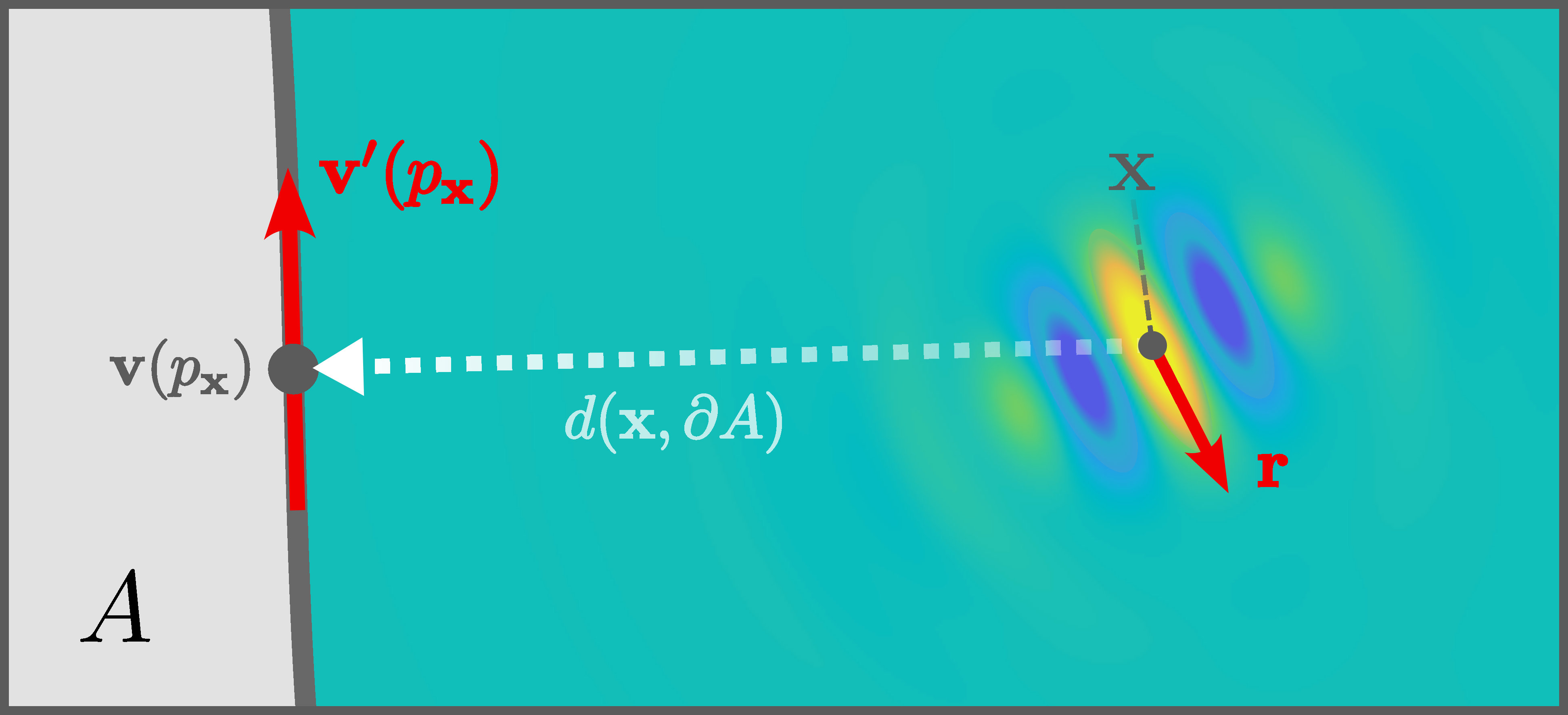
We will now state our main theorems, which reveal clear connections between geometrical properties of and the frame coefficients with respect to . As illustrated in Figure 4, it is clear that the inner products will depend heavily on both the position and orientation of the wavelet compared to the closest edge segment.
Theorem 4.3.
Let be the directional wavelet defined in (6) with , or if , where and . Then there exist constants , , as well as some nonempty open interval , such that for all with it holds that
| (27) |
and
| (28) |
The dependencies of the constants are , , and .
Roughly speaking, Theorem 4.3 states that the coefficients peak when both the position and orientation of the wavelet somewhat match the position and orientation of the nearest edge. Furthermore, these peaks remain stable in magnitude and move closer towards the boundary as increases. Away from the edge, the inner products decay rapidly.
The following theorem provides us with more insight on the structure of the frame coefficients in the vicinity of a singularity. Here, for , we make use of the notation
as well as .
Theorem 4.4.
Let be the directional wavelet defined in (6) with , or if , where . Then
| (29) |
where
holds for every with . Here, we have .
Theorem 4.4 shows how the local geometry of the boundary is reflected in the frame coefficients at high frequencies, that is, when becomes large. Most notably, the orientational dependency of the dominating term given by (4.4) is completely characterized by the directionality function . Also, the parameter only appears in the integral expression, which can be viewed as a function in that essentially gets dilated as increases.
Remark 4.5.
We note that the results presented above can be applied to all functions which are (locally) of the form , where . More precisely,
and therefore the upper and lower bounds (27) and (28) show that jump discontinuities along smooth curves can still be detected in this case. For more details on this matter we refer to the discussion in [18, Remark 1].
In order to prove Theorem 4.3 and Theorem 4.4, we will need the following result, which deals with the special case when is a spherical cap.
Theorem 4.6.
Let with and be the directional wavelet defined in (6) with for some . Then
| (30) |
where
holds for all with . Furthermore, there exist constants , , as well as some nonempty open interval , such that for all with it holds that
and
The dependencies of the constants are , , , and .
Proof.
This statement was proven in [18, Theorem 3.1] in terms of Euler angles. An adaptation of the formulas with respect to the unit tangent bundle parameterization of the rotation operator can be achieved in a straightforward manner. ∎
Another important intermediate result, which we will use to prove our main theorems, is given by the following lemma.
Lemma 4.7.
Proof.
Let with and let be the corresponding spherical cap from Lemma 4.1. We start with the simple estimate
The spatial localization bound of the directional wavelets stated in (8), or in (11) if , yields
Thus, using integration by parts, we obtain
Here, the second inequality follows from the assumption that . Additionally, if the integral can be estimated using Lemma 4.1. We obtain
It is not hard to verify that as . Indeed, since , which is a direct consequence of the famous addition theorem for spherical harmonics, the latter follows easily from the definition (6). Consequently, (31) holds. ∎
Proof of Theorem 4.3.
Let with and let be the corresponding spherical cap from Lemma 4.1. By Lemma 4.7, setting , we have
provided that . The lower bound now follows from the lower bound for spherical caps in Theorem 4.6.
Now, let . To prove the upper bound, we first consider the case . If , we can, just like in the proof of Lemma 4.7, use the localization property of to derive
| (32) |
If, on the other hand, , the fact that has a zero mean implies
and thus (32) still holds.
Finally, let . One easily verifies that . Thus, Lemma 4.7 yields
Now, the upper bound in Theorem 4.6 states that
Furthermore,
where we have used that . This completes the proof. ∎
Proof of Theorem 4.4.
We conclude this section with the following remark.
Remark 4.8.
The estimates in Theorem 4.3 and Theorem 4.4 hold, with minor modifications, also for -curves. This can be shown by using exclusively great circles in the approximation of the boundary . In particular, this approach does not take into account the curvature, which leads to a less optimal upper bound of the form
in (14). The verification of this variation of Lemma 4.1 is analogous to the original proof and, in fact, it is easier. Using this bound, one obtains essentially the same estimates as stated in Theorem 4.3, but now valid for all sets with a -boundary. Of course, one has to replace in (28) by . However, in the resulting leading term of the asymptotic formula in Theorem 4.4 one has to replace by , as unit speed parameterizations of great circles always have constant curvature equal to , which yields a less precise description of the wavelet coefficients. This is reflected in the remainder only being , , provided that .
5 Numerical example
In the previous section, we proved that jump discontinuities along smooth curves can be identified, in terms of position and orientation, by the asymptotic behavior of the corresponding frame coefficients in an arbitrary small neighborhood. By Parseval’s theorem, for a given signal it holds that
| (33) |
i.e., the wavelet coefficients are linear combinations of the Fourier coefficients of . Therefore, as a consequence of our main results, equation (33) provides a method to extract precise information about local phenomena using only the global quantities . Moreover, (33) can be utilized to compute the wavelet coefficients in practice, where the Fourier coefficients of the signal under consideration are often available.
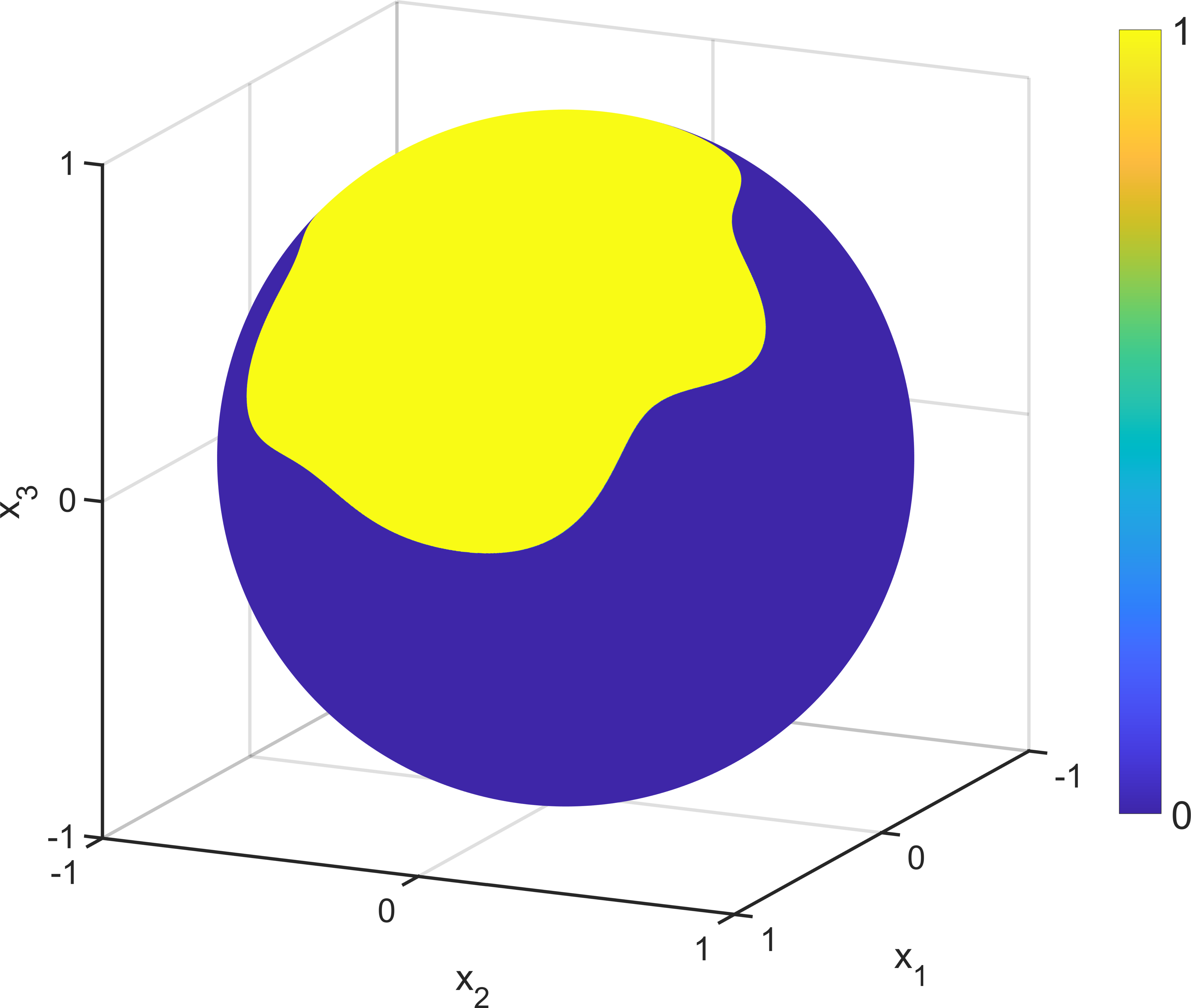
In this final section, we want to present some numerical experiments and compare the results to our theoretical findings. Let us consider the test signal , where is the set visualized in Figure 5. More precisely, with
and
Additionally we choose in (6) to be the function constructed in [7] with . As discussed in [18], it holds that
in terms of the Wigner -functions and with respect to the Euler angle parameterization of the rotation group. The above sum constitutes the Fourier synthesis of a band-limited function on the and thus can be evaluated at arbitrary points , , using fast algorithms. However, like in many practical situations, the exact Fourier coefficients of are unknown and have to be approximated using only finitely many samples. In our setting, this method inevitably leads to a certain inaccuracy since the signal is not compactly supported in frequency space.

For our experiment, we approximated the integrals by values resulting from a Gauß-Legendre quadrature rule which is exact for spherical polynomials up to degree . Subsequently, we computed the approximate wavelet coefficients
with
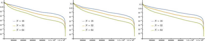
for different values of and . All computations were done in Matlab using the NFFT 3 library [4]. In Figure 6, the data points , , are visualized as functions on . Here, for the sake of clarity, all images have been re-scaled to take values between and . The magnitudes of the frame coefficients are given in Figure 7, where the absolute values are plotted in descending order. It is immediately noticeable that the coefficients become more and more concentrated along the boundary as increases. Moreover, the peaks remain stable in their magnitude and shape and, essentially, appear to just get dilated for larger values of . The directional sensitivity increases with and the area of the boundary getting detected changes with different orientations of the wavelets. Also, the parameter does not seem to affect the directional sensitivity. Hence, our observations in this numerical example are in accordance with the characteristic properties of the exact wavelet coefficients displayed in Theorem 4.3 and Theorem 4.4.
References
- Dai and Xu [2013] Dai, F., Xu, Y., 2013. Approximation theory and harmonic analysis on spheres and balls. Springer Monogr. Math., New York, NY: Springer. doi:10.1007/978-1-4614-6660-4.
- Guo and Labate [2009] Guo, K., Labate, D., 2009. Characterization and analysis of edges using the continuous shearlet transform. SIAM J. Imaging Sci. 2, 959–986. doi:10.1137/080741537.
- Guo and Labate [2018] Guo, K., Labate, D., 2018. Detection of singularities by discrete multiscale directional representations. J. Geom. Anal. 28, 2102–2128. doi:10.1007/s12220-017-9897-x.
- Keiner et al. [2009] Keiner, J., Kunis, S., Potts, D., 2009. Using nfft 3—a software library for various nonequispaced fast fourier transforms. ACM Trans. Math. Softw. 36. doi:10.1145/1555386.1555388.
- Khabiboulline and Prestin [2006] Khabiboulline, R., Prestin, J., 2006. Asymptotic formulas for the frame coefficients generated by Laguerre and Hermite type polynomials. Int. J. Wavelets Multiresolut. Inf. Process. 4, 415–431. doi:10.1142/S0219691306001348.
- Kutyniok and Petersen [2017] Kutyniok, G., Petersen, P., 2017. Classification of edges using compactly supported shearlets. Appl. Comput. Harmon. Anal. 42, 245–293. doi:10.1016/j.acha.2015.08.006.
- McEwen et al. [2018] McEwen, J.D., Durastanti, C., Wiaux, Y., 2018. Localisation of directional scale-discretised wavelets on the sphere. Appl. Comput. Harmon. Anal. 44, 59–88. doi:10.1016/j.acha.2016.03.009.
- McEwen et al. [2013] McEwen, J.D., Vandergheynst, P., Wiaux, Y., 2013. On the computation of directional scale-discretized wavelet transforms on the sphere, in: Wavelets and Sparsity XV, SPIE international symposium on optics and photonics, invited contribution. doi:10.1117/12.2022889.
- Mhaskar et al. [2000] Mhaskar, H.N., Narcowich, F.J., Prestin, J., Ward, J.D., 2000. Polynomial frames on the sphere. Adv. Comput. Math. 13, 387–403. doi:10.1023/A:1016639802349.
- Mhaskar and Prestin [1999] Mhaskar, H.N., Prestin, J., 1999. On a build-up polynomial frame for the detection of singularities, in: Self-similar systems. Proceedings of the international workshop, Dubna, Russia, July 30–August 7, 1998. Dubna: Joint Institute for Nuclear Research, pp. 98–109.
- Mhaskar and Prestin [2000a] Mhaskar, H.N., Prestin, J., 2000a. On the detection of singularities of a periodic function. Adv. Comput. Math. 12, 95–131. doi:10.1023/A:1018921319865.
- Mhaskar and Prestin [2000b] Mhaskar, H.N., Prestin, J., 2000b. Polynomial frames for the detection of singularities, in: Wavelet analysis and multiresolution methods. Proceedings of the conference, University of Illinois, Urbana-Champaign, IL, USA. New York, NY: Marcel Dekker, pp. 273–298.
- Narcowich et al. [2006] Narcowich, F., Petrushev, P., Ward, J., 2006. Decomposition of Besov and Triebel-Lizorkin spaces on the sphere. J. Funct. Anal. 238, 530–564. doi:10.1016/j.jfa.2006.02.011.
- Narcowich et al. [2007] Narcowich, F.J., Petrushev, P., Ward, J.D., 2007. Localized tight frames on spheres. SIAM J. Math. Anal. 38, 574–594. doi:10.1137/040614359.
- Petrushev and Xu [2005] Petrushev, P., Xu, Y., 2005. Localized polynomial frames on the interval with Jacobi weights. J. Fourier Anal. Appl. 11, 557–575. doi:10.1007/s00041-005-4072-3.
- Schober and Prestin [2023] Schober, K., Prestin, J., 2023. Analysis of directional higher order jump discontinuities with trigonometric shearlets. Math. Found. Comput. 6, 14–40. doi:10.3934/mfc.2021038.
- Schober et al. [2021] Schober, K., Prestin, J., Stasyuk, S.A., 2021. Edge detection with trigonometric polynomial shearlets. Adv. Comput. Math. 47, 41. doi:10.1007/s10444-020-09838-3. id/No 17.
- Schoppert [2023] Schoppert, F., 2023. Direction sensitive analysis of higher order jump discontinuities along circles on the sphere. GEM. Int. J. Geomath. 14, 33. doi:10.1007/s13137-023-00217-w. id/No 7.
- Wiaux et al. [2008] Wiaux, Y., McEwen, J.D., Vandergheynst, P., Blanc, O., 2008. Exact reconstruction with directional wavelets on the sphere. Mon. Not. Roy. Astron. Soc. 388, 770–788. doi:10.1111/j.1365-2966.2008.13448.x.