Thinning a Wishart Random Matrix
Abstract
Recent work has explored data thinning, a generalization of sample splitting that involves decomposing a (possibly matrix-valued) random variable into independent components. In the special case of a random matrix with independent and identically distributed rows, Dharamshi et al. (2024a) provides a comprehensive analysis of the settings in which thinning is or is not possible: briefly, if is unknown, then one can thin provided that . However, in some situations a data analyst may not have direct access to the data itself. For example, to preserve individuals’ privacy, a data bank may provide only summary statistics such as the sample mean and sample covariance matrix. While the sample mean follows a Gaussian distribution, the sample covariance follows (up to scaling) a Wishart distribution, for which no thinning strategies have yet been proposed. In this note, we fill this gap: we show that it is possible to generate two independent data matrices with independent rows, based only on the sample mean and sample covariance matrix. These independent data matrices can either be used directly within a train-test paradigm, or can be used to derive independent summary statistics. Furthermore, they can be recombined to yield the original sample mean and sample covariance.
1 Introduction
Many modern data analysis pipelines rely on the ability to split a dataset into independent parts. For instance, one might wish to fit a model to one part and validate it on another, or else to select a parameter of interest on one part and conduct inference on the other. In cases where we have access to independent and identically distributed observations, sample splitting provides a simple strategy to split our data into independent parts (Cox, 1975). However, in some settings, sample splitting is either inapplicable or unattractive. For instance, perhaps the observations are not independent or not identically distributed, or perhaps .
In a recent line of work, a number of authors have considered alternatives to sample splitting that involve splitting a single (possibly matrix-valued) random variable into independent random variables, which can be recombined to yield the original random variable. We refer to such strategies, in aggregate, as data thinning: see Definition 1 of Dharamshi et al. (2024b). Robins & van der Vaart (2006), Tian & Taylor (2018), Rasines & Young (2023), and Leiner et al. (2023) show that it is possible to thin a random vector with unknown and known. Neufeld et al. (2024) extended this strategy to natural exponential families, such as the binomial family and the negative binomial family with known overdispersion parameter. Dharamshi et al. (2024b) clarified the class of distributions that can be thinned, and showed that it extends far beyond natural exponential families, to examples such as the uniform and beta families.
Dharamshi et al. (2024a) outlines the following possibilities for thinning independent and identically distributed random variables:
In contrast to prior work, in this note we consider a situation in which we do not actually have access to the original sample of random variables: that is, are unobserved. Instead, we only have access to the summary statistics, the sample mean and the sample covariance :
| (1) |
This may be the case for one of the following reasons:
-
1.
Privacy considerations may preclude the release of ; however, and can be released. For instance, in the context of genetic data, it is often not possible to share the raw data. Instead, summary statistics — which are typically less personally identifiable — of the data are shared. As one example, Pasaniuc & Price (2017) discuss the release of a correlation matrix between genetic variants in cases where individual-level data cannot be shared due to privacy concerns.
-
2.
The data analysis pipeline requires only the summary statistics, and the data analyst does not have access to the original data . This may be due to scientific considerations: for example, in the context of neuroscience research, analyses often center on the matrix of connectivity between voxels of the brain (Cohen et al., 2017). Or it might be due to statistical considerations: for example, the graphical lasso proposal (Friedman et al., 2008) operates on the sample covariance matrix, not the matrix normal data matrix from which it arose. Or alternatively, perhaps the matrix was measured directly, i.e. there is no , as in classical multidimensional scaling (Torgerson, 1952).
Classical results in multivariate statistics tell us that and , the -dimensional Wishart distribution with degrees of freedom (see Remark 1). In this note, we develop a thinning strategy to create two or more independent random matrices with independent rows from these summary statistics. The key technical result making this possible is a procedure, which we introduce in Section 2, that is originally due to Lindqvist & Taraldsen (2005). We go on to show how this result can be used to thin a Wishart distribution into two (or more) Wisharts, thereby adding a new entry into the list of natural exponential families where convolution-closed thinning (Neufeld et al., 2024) is known to be possible.
Henceforth, we will use the notation to denote the matrix normal distribution with rows, columns, mean matrix , row-covariance matrix , and column-covariance matrix . Moreover, we will use the notation to indicate the uniform distribution on the set of orthogonal matrices. This is known as the Haar invariant distribution (on ) (Anderson, 2003; Muirhead, 2009).
Remark 1.
When , follows a singular Wishart distribution (Srivastava, 2003); the distinction between the singular and non-singular Wishart distributions is not important in what follows and thus we will use the word “Wishart” throughout.
2 A matrix square root of a Wishart with independent Gaussian rows
Given a rank- matrix , if the matrix satisfies , then we say that is a matrix square root of . (Of course, it must be the case that .) The matrix square root is not unique. For example, consider the eigenvalue decomposition , where is a diagonal matrix and is a orthogonal matrix: then for any orthogonal matrix , it follows that is a matrix square root of .
By definition, a Wishart random matrix has a matrix square root with rows that are independent and identically distributed multivariate Gaussians. One might hope that any matrix square root of a Wishart matrix would have this property, but this is not the case (see, e.g. Section 4.1). To achieve this property, we present Algorithm 2. Theorem 1 that follows shows that this algorithm generates matrix square roots with independent and identically distributed Gaussian rows.
[!h]
Theorem 1 (A square root of a Wishart with independent Gaussian rows).
Suppose that we apply Algorithm 2 to , where , to obtain an matrix . Then, , and the rows of are independent random variables.
In the next section, we will show that Theorem 1 can be applied to thin the summary statistics of an unobserved sample of independent and identically distributed Gaussian vectors.
3 Thinning the sample covariance
We return now to the setting of this paper, where denote a sample of independent Gaussian vectors that are unavailable to the data analyst.
3.1 The case where is known
We first consider the case where is known, and the analyst is provided with
| (2) |
along with the sample size . The following corollary of Theorem 1 enables us to thin into independent Wishart random matrices.
Corollary 1 (Thinning the sample covariance of independent Gaussians with known mean).
Suppose that we apply Algorithm 2 to to obtain an matrix , where is defined in (2) for . Then, (i) , and (ii) the rows of are independent random variables. Furthermore, let denote a partition of the integers such that for any and , and define where is the number of elements in the set . Then, (iii) and are independent.
Proof.
Noting that , (i) and (ii) follow immediately from Theorem 1. Furthermore, (iii) follows from the independence of the rows of , as well as the definition of the Wishart distribution. ∎
What is the point of Corollary 1? Given the sample covariance matrix from a sample of independent random vectors, we can obtain either (a) independent normal data matrices , where , or (b) independent sample covariance matrices corresponding to those data matrices. We can use (a) in order to conduct a data analysis pipeline, such as cross-validation, that requires multiple independent data folds. We can use (b) if the data analysis pipeline specifically requires sample covariance matrices. In either case, the independent random variables obtained can be re-combined to yield the original sample covariance matrix.
3.2 The case where is unknown
We now turn to the case where the mean vector is unknown, and the data analyst is given access to and from (1), along with the sample size . The next result establishes that Algorithm 3.2, a variant of Algorithm 2, can be applied to thin .
[!h]
Theorem 2 (Thinning the sample covariance and sample mean of independent Gaussians).
Suppose that we apply Algorithm 3.2 to to obtain an matrix , where and are defined in (1) for . Then, (i) and , and (ii) the rows of are independent random variables. Furthermore, let denote a partition of the integers such that for any and , and define and , where is the number of elements in the set . Then, (iii) , , and are independent.
4 Numerical Results
4.1 Verification of Theorems 1 and 2
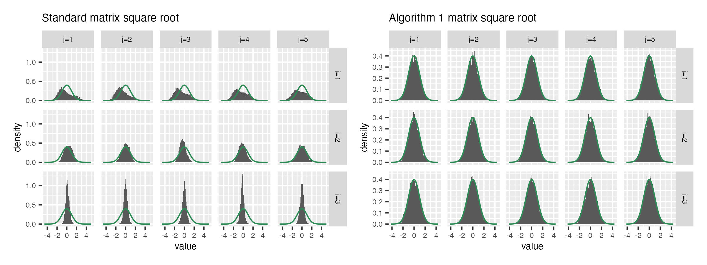
Theorem 1 establishes that applying Algorithm 2 to a Wishart matrix will generate a matrix square root whose rows are independent Gaussian random vectors. In this section, we demonstrate in a numerical example that this is the case, and draw a contrast to another matrix square root that does not share this property.
Setting and , we first construct a matrix with a Toeplitz structure, , and draw by generating and then computing . Let denote the eigendecomposition of , and define . Define to be the output of Step 3 of Algorithm 2 applied to . Figure 1 compares the entry-wise marginal distributions of and . In particular, each panel contains an array of histograms, the th of which displays the distribution of (left) or (right) across 10,000 repetitions. Superimposed on each histogram is the desired marginal distribution, . We can see that the entries of are far from normal, whereas the entries of have the correct marginals.
4.2 Application to post-selective inference in the graphical lasso
The graphical lasso (Yuan & Lin, 2007; Banerjee et al., 2008; Rothman et al., 2008; Friedman et al., 2008) estimator of the precision matrix is
| (3) |
for defined in (1). Provided that arose from a sample of independent and identically distributed Gaussian random vectors, minimizes the negative log likelihood subject to an penalty on the elements of the precision matrix. Here, is a nonnegative tuning parameter that determines the sparsity of . In this section, we consider selecting via cross-validation.
If we have access to the Gaussian random vectors used to compute , then we can use sample splitting to instantiate a cross-validation scheme to select . In greater detail, let denote a partition of such that and . Then, for , we define and to be the sample covariance matrices computed on the observations in and on all but the observations in , respectively (where and are the corresponding sample means). We let denote the graphical lasso estimator computed on . We select the value of that minimizes
Now, suppose that — following the setup of this paper — we do not have access to directly, but only to from (1). Consequently, cross-validation via sample splitting cannot be applied. Instead, we apply Algorithm 2 to to obtain an matrix ; here, we use in place of because has rank . By Theorem 1, the rows of this matrix are independent random vectors. We then partition the indices into , where and . We define and . Note that , and that and are independent.
For , we let denote the graphical lasso estimator computed on , with tuning parameter . We then select the value of that minimizes
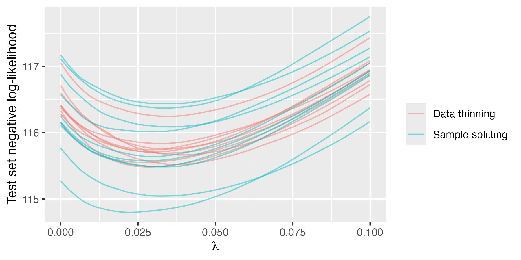
We now compare and in simulation. We generate independent random vectors where , , and is block diagonal, with blocks , , and . Figure 2 displays and for , for each of ten simulated datasets. We find that all curves are minimized when . Therefore, data thinning selects the same tuning parameter as sample splitting, without requiring access to the individual-level data .
5 Discussion
Arguments from Neufeld et al. (2024) and Dharamshi et al. (2024b) suggest that it might be possible to thin a random matrix into independent Wishart random matrices , with for , by sampling from the conditional distribution of given . Since is sufficient for , sampling from this conditional distribution does not require knowledge of . It turns out that this conditional distribution is closely related to the matrix variate Dirichlet distribution (Gupta & Nagar, 2018). In fact, an alternative to the procedure described in Corollary 1 can be obtained by sampling from this conditional distribution.
Code to reproduce all numerical analyses in this note is available at https://github.com/AmeerD/Wishart/.
References
- (1)
- Anderson (2003) Anderson, T. W. (2003), An Introduction to Multivariate Statistical Analysis, Vol. 3, Wiley New York.
- Banerjee et al. (2008) Banerjee, O., El Ghaoui, L. & d’Aspremont, A. (2008), ‘Model selection through sparse maximum likelihood estimation for multivariate Gaussian or binary data’, Journal of Machine Learning Research 9, 485–516.
- Cohen et al. (2017) Cohen, J. D., Daw, N., Engelhardt, B., Hasson, U., Li, K., Niv, Y., Norman, K. A., Pillow, J., Ramadge, P. J., Turk-Browne, N. B. et al. (2017), ‘Computational approaches to fMRI analysis’, Nature Neuroscience 20(3), 304–313.
- Cox (1975) Cox, D. R. (1975), ‘A note on data-splitting for the evaluation of significance levels’, Biometrika 62(2), 441–444.
- Dharamshi et al. (2024a) Dharamshi, A., Neufeld, A., Gao, L. L., Bien, J. & Witten, D. (2024a), ‘Decomposing Gaussians with unknown covariance’, arXiv preprint arXiv:2409.11497 .
- Dharamshi et al. (2024b) Dharamshi, A., Neufeld, A., Motwani, K., Gao, L. L., Witten, D. & Bien, J. (2024b), ‘Generalized data thinning using sufficient statistics’, Journal of the American Statistical Association (just-accepted), 1–13.
- Friedman et al. (2008) Friedman, J., Hastie, T. & Tibshirani, R. (2008), ‘Sparse inverse covariance estimation with the graphical lasso’, Biostatistics 9(3), 432–441.
- Gupta & Nagar (2018) Gupta, A. K. & Nagar, D. K. (2018), Matrix variate distributions, Chapman and Hall/CRC.
- James (1954) James, A. T. (1954), ‘Normal multivariate analysis and the orthogonal group’, The Annals of Mathematical Statistics 25(1), 40–75.
- Leiner et al. (2023) Leiner, J., Duan, B., Wasserman, L. & Ramdas, A. (2023), ‘Data fission: splitting a single data point’, Journal of the American Statistical Association pp. 1–12.
- Lindqvist & Taraldsen (2005) Lindqvist, B. H. & Taraldsen, G. (2005), ‘Monte Carlo conditioning on a sufficient statistic’, Biometrika 92(2), 451–464.
- Muirhead (2009) Muirhead, R. J. (2009), Aspects of Multivariate Statistical Theory, John Wiley & Sons.
- Neufeld et al. (2024) Neufeld, A., Dharamshi, A., Gao, L. L. & Witten, D. (2024), ‘Data thinning for convolution-closed distributions’, Journal of Machine Learning Research 25(57), 1–35.
- Pasaniuc & Price (2017) Pasaniuc, B. & Price, A. L. (2017), ‘Dissecting the genetics of complex traits using summary association statistics’, Nature Reviews Genetics 18(2), 117–127.
- Rasines & Young (2023) Rasines, D. G. & Young, G. A. (2023), ‘Splitting strategies for post-selection inference’, Biometrika 110(3), 597–614.
- Rennie (2006) Rennie, J. (2006), ‘Jacobian of the singular value decomposition with application to the trace norm distribution’.
-
Robins & van der Vaart (2006)
Robins, J. & van der Vaart, A. (2006), ‘Adaptive nonparametric confidence sets’, The Annals of Statistics 34(1), 229 – 253.
https://doi.org/10.1214/009053605000000877 -
Rothman et al. (2008)
Rothman, A. J., Bickel, P. J., Levina, E. & Zhu, J. (2008), ‘Sparse permutation invariant covariance estimation’, Electronic Journal of Statistics 2(none), 494 – 515.
https://doi.org/10.1214/08-EJS176 - Srivastava (2003) Srivastava, M. S. (2003), ‘Singular Wishart and multivariate beta distributions’, The Annals of Statistics 31(5), 1537–1560.
- Tian & Taylor (2018) Tian, X. & Taylor, J. (2018), ‘Selective inference with a randomized response’, The Annals of Statistics 46(2), 679–710.
- Torgerson (1952) Torgerson, W. S. (1952), ‘Multidimensional scaling: I. theory and method’, Psychometrika 17(4), 401–419.
- Yuan & Lin (2007) Yuan, M. & Lin, Y. (2007), ‘Model selection and estimation in the Gaussian graphical model’, Biometrika 94(1), 19–35.
Appendix A Proof of Theorem 1
Proof.
We start by noting that . It remains to show that has the desired distribution. This will follow from some facts about the matrix normal.
Consider an random matrix , and denote its singular value decomposition as . By definition of the Wishart distribution, has the same distribution as . Thus, and from the eigenvalue decomposition of in Step 1 have the same joint distribution as and . It remains to show the following two claims:
-
Claim 1.
; and
-
Claim 2.
is distributed uniformly on the Stiefel manifold, where .
Provided that these two claims hold, has the same distribution as , and so the proof is complete.
It remains to justify the two claims. When , both claims follow directly from James (1954). For , we will show that the joint density of factors into the desired terms. Following the transformation , the joint density of simplifies as
where indicates the Jacobian of the transformation, are the singular values, and refers to the wedge product (see Rennie 2006 for details on the wedge product). For details on the derivation of the Jacobian, see Srivastava (2003) and Rennie (2006). Notice that factors into and . This implies that is independent of and . Further, the fact that implies that is uniformly distributed on the Stiefel manifold (Anderson 2003, Muirhead 2009). Thus, both claims are proven when .
∎
Appendix B Proof of Theorem 2
Proof.
We begin by verifying (i): namely, that and .
First, recalling from Algorithm 3.2 that is an orthogonal matrix such that , note that . Therefore, .
Recalling the construction of from applying Algorithm 3.2 with , observe that
where the last equality follows from the fact that . Furthermore,
since and . Noting that is idempotent, we have that
where the second-to-last equality follows from the fact that and , and the last equality follows from Step 1 of Algorithm 3.2.
We will now establish (ii): namely, that has the desired distribution. First, note that . Next, observe that the generated in Step 3 of Algorithm 3.2 is exactly the output of calling Algorithm 2 with in place of (this is allowed since Algorithm 3.2 requires whereas Algorithm 2 requires ). Therefore, . Recalling that and that depends only on , we have that . Thus, . Writing in matrix form,
establishes that is a linear transformation of a matrix normal and therefore is itself matrix normal, with mean and row and column covariance matrices and , respectively.
It remains to establish (iii): namely, that and are independent. The independence of follows immediately from the fact that the rows of are independent and form a partition. To establish that , first observe that , where is the submatrix of containing the rows of corresponding to . Furthermore, define to be a orthogonal matrix with . Because , it follows that is . ∎
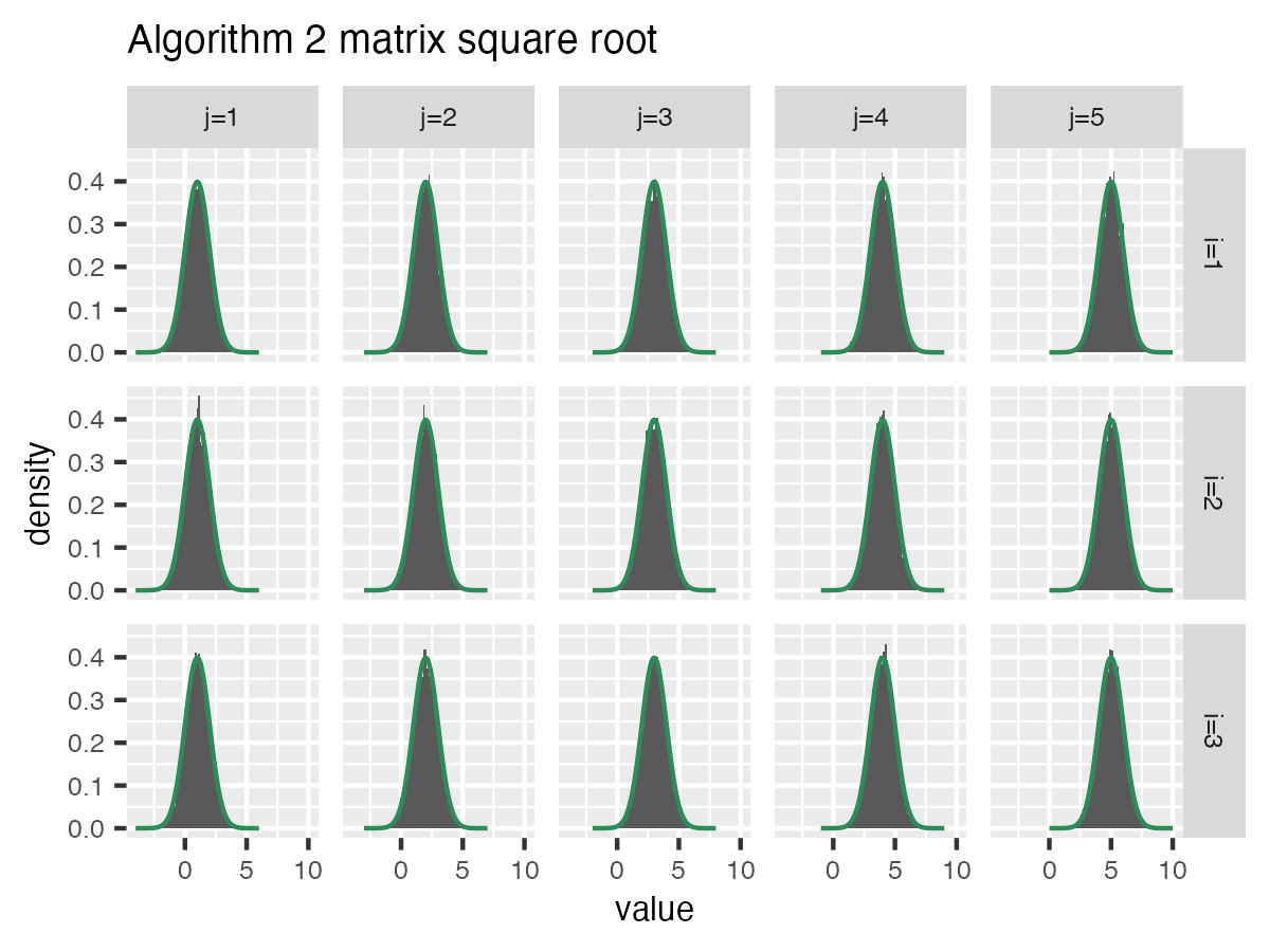
Appendix C Additional numerical experiments
We conduct a second simulation study similar to that of Section 4.1, though with unknown . Again, we set and , and construct a length vector such that the th entry , and a matrix with a Toeplitz structure, . We then generate , and compute and . Let be the output of Step 3 of Algorithm 3.2 applied to . Figure 3 displays the marginal distributions of the elements of . Each panel contains an array of histograms, the th of which displays the distribution of across 10,000 repetitions. Superimposed on each histogram is the desired marginal distribution, . We can see that the entries of have the correct marginals, thereby numerically verifying Theorem 2.