Towards Seamless Hierarchical Federated Learning under Intermittent Client Participation: A Stagewise Decision-Making Methodology

Abstract

Federated Learning (FL) offers a pioneering distributed learning paradigm that enables devices/clients to build a shared global model. This global model is obtained through frequent model transmissions between clients and a central server, which may cause high latency, energy consumption, and congestion over backhaul links. To overcome these drawbacks, Hierarchical Federated Learning (HFL) has emerged, which organizes clients into multiple clusters and utilizes edge nodes (e.g., edge servers) for intermediate model aggregations between clients and the central server. Current research on HFL mainly focus on enhancing model accuracy, latency, and energy consumption in scenarios with a stable/fixed set of clients. However, addressing the dynamic availability of clients – a critical aspect of real-world scenarios – remains underexplored. This study delves into optimizing client selection and client-to-edge associations in HFL under intermittent client participation so as to minimize overall system costs (i.e., delay and energy), while achieving fast model convergence. We unveil that achieving this goal involves solving a complex NP-hard problem. To tackle this, we propose a stagewise methodology that splits the solution into two stages, referred to as Plan A and Plan B. Plan A focuses on identifying long-term clients with high chance of participation in subsequent model training rounds. Plan B serves as a backup, selecting alternative clients when long-term clients are unavailable during model training rounds. This stagewise methodology offers a fresh perspective on client selection that can enhance both HFL and conventional FL via enabling low-overhead decision-making processes. Through evaluations on MNIST and CIFAR-10 datasets, we show that our methodology outperforms existing benchmarks in terms of model accuracy and system costs.

1 Introduction

The proliferation of smart devices has led to the generation of massive amounts of data, fueling the rise of artificial intelligence (AI)/machine learning (ML) applications across Internet-of-Things (IoT) ecosystem [1]. Conventional AI/ML methods typically involve pooling the data of distributed IoT devices at a central location (e.g., a server) for model training. However, privacy regulations often restrict the transfer of devices’ data across the network. This has triggered a paradigm shift from centralized to distributed AI/ML methods, with federated learning (FL) [3, 4, 43] emerging as a common approach. FL starts with a central server, e.g., a cloud server (CS), broadcasting a global model to clients (e.g., mobile devices). Subsequently, each client first synchronizes its local model with the global model and then trains its local model on its data (e.g., via gradient descent). Each client then uploads its local model parameters back to the server. The server finally aggregates the received models to update the global model (e.g., via weighted averaging). This process of local training and global model aggregations continues until reaching the desired performance [2].

FL naturally relies on frequent model transmissions between clients and the CS, which can incur high overhead (e.g., latency and energy) [5, 6, 7]. Hierarchical FL (HFL) is a well-recognized framework to address this challenge [8, 9]. HFL introduces an intermediate layer to the model training architecture of FL for intermediate model aggregations (a layer of edge servers (ESs)), that synchronize the model parameters of their associated clients frequently, and exchange model updates with the CS with a lower frequency [10].

1.1 Motivation and Research Direction

Although HFL has tremendous potentials in enhancing the time and energy efficiency of FL, its implementation in large-scale, dynamic networks (e.g., with mobile devices acting as clients and multiple ESs) faces unexplored challenges. We identify and study three major research questions: i) How to actively select/recruit the dynamic and resource-constrained clients to achieve cost-efficiency (e.g., reducing the training delay and energy consumption)? Due to limited bandwidth availability, only a subset of clients can be selected/recruited for interactions with ESs [12]. The intermittent availability and heterogeneity of clients (i.e., varying computational and communication capabilities), as well as differences in their data qualities can further complicate the client selection [11]. ii) How to associate the selected clients to proper ESs to achieve resource-efficiency and acceleration of model convergence? Given a set of selected clients, different client-to-edge (C2E) association strategies can significantly influence the model convergence, due to non-independent and identically distributed (non-IID) nature of data across clients [13]. We hypothesize that optimal convergence occurs when the C2E association results in clusters of devices at each ES having a collective data distribution closely resembling the global dataset spread across all clients. This aligns with the intuition that effective device clustering should mitigate clients’ local model biases during local model aggregations with ESs. This not only accelerates convergence but also diminishes the reliance on resource-intensive edge-to-cloud model aggregations, echoing observations noted in prior research [8, 10, 14]. iii) How to expedite the overall decision-making process required for determining client selection and C2E association (i.e., reduce the decision-making overhead)? The dynamics of client availability, varying local workloads, and individual selfishness necessitate frequent decision-making at the network operator level, such as at each global model training round in HFL. The requirement for constant decision-making regarding the client recruitment and C2E association can lead to significant overhead (i.e., increased latency and energy consumption). Thus, such frequent decision-making can disrupt the training process and complicate the necessary synchronizations within the training period.

1.2 Overview and Summary of Contributions

We study HFL over device-edge-cloud continuum with intermittent client participation. In this setting, due to the intermittent availability of clients, the decisions on client selection and C2E association need to be re-evaluated frequently. We subsequently focus on reducing the overhead of decision-making, an area which is underexplored in both FL and HFL broadly. In doing so, we solve the problem of joint client selection and C2E association by proposing a low-overhead stagewise decision-making methodology. In a nutshell, our methodology aims to shift the burden of online decision-making – as done in almost all the literature of FL and HFL – to aforehand/offline decision-making, which can significantly accelerate the execution of model training. Additionally, since relying solely on offline decision-making could compromise the practicality of the approach due to system dynamics, our method incorporates minimal online decision-making to refine the offline decisions. Our major contributions can be summarized as follows:

$\bullet$ We are interested in addressing the challenge of joint client selection and C2E association for HFL under intermittent client participation, by formulating an NP-hard optimization problem that minimizes system costs while effectively managing data heterogeneity.

$\bullet$ To manage complexity, we propose a novel stagewise methodology that decouples the problem into two parts: Plan A identifies potential clients for future training, while Plan B ensures seamless execution if those clients become unavailable.

$\bullet$ In Plan A, we introduce the concept of “client continuity” and derive closed-form constraints on tolerable data heterogeneity, modeled probabilistically. To identify suitable long-term clients, we propose a strategy that combines gain-of-cost minimization-promoted C2E association and local iteration-based determination. While in Plan B, we refine Plan A’s decisions when long-term clients become unavailable, and introduce a cluster-based client update algorithm for the rapid exploration of suitable alternative clients in an online manner.

$\bullet$ Extensive experiments on datasets such as MNIST, Fashion-MNIST, CIFAR-10 and CIFAR-100 validate the effectiveness of our approach in improving model accuracy, system cost, and time efficiency.

2 Related Work

Numerous studies investigated balancing the model training performance (e.g., model accuracy) and cost-effectiveness for FL. For example, [15, 16, 17] study model compression, gradient quantization, and coding techniques to reduce the model aggregation overhead. Also, [18, 19, 20] conduct communication/computation resource allocation for FL. Further, [21, 22] aim to reduce the required global aggregation rounds. These works study FL with direct client-to-cloud communications, which can cause causing increased latency, energy consumption, and congestion over the backhaul links.

To address the above discussed issues, HFL was proposed by Liu et al. [8], introducing an intermediate aggregation layer (e.g., formed by ESs) to reduce the frequency of direct communications between clients and the remote cloud. Luo et al. [5] further conducted resource allocation and C2E association for HFL. Feng et al. [24] optimized subcarrier assignment, transmit power of clients, and computation resources in HFL. Lin et al. [25] proposed control algorithms for delay-aware HFL, obtaining policies to mitigate communication latency in HFL.

Considering the constraints of limited resources in wireless networks, developing a joint client selection and C2E association strategy for HFL training emerges as a viable approach to enhance model training efficiency, which has attracted wide research attentions in recent years. For example, Deng et al. [10] minimized the total communication cost required for model learning with a target accuracy, by making decisions on edge aggregator selection and node-edge associations a the HFL framework. Su et al. [26] developed an online learning-based client selection algorithm for ESs, based on empirical learning results, reducing the cumulative delay on computation and communication. Qu et al. [27] observed the context of local computing and transmission of client-ES pairs, making client selection decisions to maximize the network operator’s utility, under a given budget.

Besides HFL, several novel FL architectures have been proposed to address the high communication overhead caused by frequent interactions with the remote server. For example, Guo et al. [56] proposed a hybrid local SGD (HL-SGD) algorithm, which leverages the availability of fast D2D links to accelerate convergence and reduce training time under non-IID data distributions. However, similar to traditional FL and HFL, the central entity in HL-SGD may still become a bottleneck and suffer from a single point of failure, raising concerns about fault tolerance and scalability. To tackle this issue, a cooperative federated edge learning (CFEL) [57, 58] framework was introduced, which exploits multiple aggregators and eliminates single points of failure, making it more scalable than prior FL frameworks. Castiglia et al. [57] proposed Multi-Level Local SGD (MLL-SGD) in a two-tier communication network with heterogeneous workers, but their work is limited to IID data distributions. Zhang et al. [58] further designed a new federated optimization method called cooperative edge-based federated averaging (CE-FedAvg), which efficiently learns a shared global model over the collective dataset with non-IID data of all edge devices under the orchestration of a distributed network of cooperative edge servers.

The above existing studies have made valuable contributions in the realm of model training by enhancing client participation and optimizing network orchestration. These contributions have laid a strong foundation for improving the efficiency and effectiveness of federated learning systems. However, many of these works either assume that clients are consistently available for model training or do not fully account for the decision-making overhead associated with client recruitment and network orchestration. However, many of these works either assume that clients are consistently available for model training or do not fully account for the decision-making overhead associated with client recruitment and network orchestration. Specifically, the time required to select clients and establish their association with ESs are often overlooked. Addressing these factors is crucial for the practical implementation of HFL, particularly in dynamic and resource-constrained environments. This work explores an unexplored research angle and contributes to the on-going research by proposing stagewise decision-making for HFL under intermittent client availability. Interestingly, it employs two complementary plans for client selection and C2E association executed at different timescales to ensure a seamless and efficient model training process.

3 System Model

Figure 1: A schematic of stagewise desicion-making for HFL over dynamic device-edge-cloud continuum with intermittent client participation.

As shown in Fig. 1, we consider hierarchical federated learning (HFL) over a three-layer network hierarchy including i) a cloud server (CS) acting as the centralized aggregator, ii) several edge servers (ESs), denoted by $\mathcal{S}=\left\{s_{1},\ldots,s_{j},\ldots,s_{|\mathcal{S}|}\right\}$, acting as intermediate aggregators, and iii) a set of mobile devices (clients) $\mathcal{N}=\left\{\bm{n}_{1},\ldots,\bm{n}_{i},\ldots,\bm{n}_{|\mathcal{N}|}\right\}$. Each client $\bm{n}_{i}\in\mathcal{N}$ is described via a 4-tuple $\bm{n}_{i}=[\mathcal{D}_{i},v_{i},q_{i},\xi_{i}]$, where $\mathcal{D}_{i}=\left\{\left(\boldsymbol{x}_{1},y_{1}\right),\ldots,\left(\boldsymbol{x}_{k},y_{k}\right),\ldots,\left(\boldsymbol{x}_{\left|\mathcal{D}_{i}\right|},y_{\left|\mathcal{D}_{i}\right|}\right)\right\}$ denotes its local dataset and $\boldsymbol{x}_{k}$ and $y_{k}$ denote the input feature and label of the $k^{\text{th}}$ datapoint, respectively. Let ${\mathcal{D}=\left\{\mathcal{D}_{1},\ldots,\mathcal{D}_{i},\ldots,\mathcal{D}_{|\mathcal{N}|}\right\}}$ encapsulate the dataset profile of clients. Also, let $v_{i}$ denote the computation capability of $\bm{n}_{i}$ (i.e., its CPU frequency), and $q_{i}$ represent the transmit power of $\bm{n}_{i}$. Learning takes place through a sequence of global and local model aggregations, where the index of an arbitrary global model aggregation is denoted by $g$ and the index of an arbitrary local aggregation is denoted by $\ell$. We capture the intermittent client availability across global aggregations via $\xi_{i}^{(g)}$, which is an indicator function for describing the participation of client $\bm{n}_{i}\in\mathcal{N}$. In particular, $\xi_{i}^{(g)}=1$ indicates that $\bm{n}_{i}$ takes part in the $g^{\text{th}}$ global aggregation, and $\xi_{i}^{(g)}=0$, otherwise ($\xi_{i}^{(g)}$ is detailed in Sec. 3.3).

Each global aggregation of HFL starts with broadcasting the global model from CS to clients, with ESs acting as relays. Afterwards, clients synchronize their local models with the global model, train their local models on their datasets, and then upload their model parameters to their assigned ESs. After aggregating the received models from their clients (i.e., conducting local model aggregation), ESs have two options: i) broadcasting the aggregated edge model back to their clients for another round of local model training (i.e., conclusion of one local/edge aggregation round); ii) sending the aggregated edge model to the CS for global aggregation (i.e., conclusion of one global aggregation round). This procedure calls for addressing both client recruitment/selection (i.e., determining proper clients for training) and client-to-edge (C2E) association (i.e., assigning clients to proper ESs), which given their combinatorial natures are NP-Hard (discussed in Sec. 4). Thus, the overhead of solving these problems can become unacceptable in large-scale networks, affecting the sustainability and practicality of HFL.

Subsequently, our primary goal is to recruit clients and assign them to appropriate ESs at each global aggregation round, while ensuring i) the reliability and performance of the system, meaning seamless execution of HFL with an adequate number of clients and fast convergence of the trained global model; ii) low decision-making overhead, which involves minimizing the time spent on online decision-making to maximize the time available for model training; iii) reduced costs (i.e., energy consumption and latency) of model training. We achieve this goal via a stagewise decision-making process, consisting of Plan A and Plan B, where in Plan A, a set of long-term clients (often those with higher probabilities of participation in model training) are selected for future global model aggregations in an offline manner. Also, Plan B involves online recruitment and orchestration of short-term clients to compensate for long-term ones that are unavailable at each practical global aggregation round. Notations are summarized in App. A.

3.1 Modeling of HFL Procedure

We introduce $\boldsymbol{A}^{(g)}=\left\{a_{i,j}^{(g)}\mid\bm{n}_{i}\in\mathcal{N},s_{j}\in\mathcal{S}\right\}$, where $a_{i,j}^{(g)}=1$ if client $\bm{n}_{i}$ is selected/recruited and associated with ES $s_{j}$; otherwise $a_{i,j}^{(g)}=0$. We next formalize different HFL steps.

$\bullet$ Step 1: Let $\bm{\omega}_{i}^{(g;\ell,t)}$ denote the local model of client $\bm{n}_{i}$, at edge aggregation round $\ell$ ($0\leq\ell\leq\mathcal{L}-1$), where $t$ is the index for local updates. After receiving the global model $\bm{\omega}^{(g)}$ broadcasted by CS at global aggregation $g$, each client $\bm{n}_{i}$ first synchronizes its local model as $\bm{\omega}_{i}^{(g;0,0)}\leftarrow\bm{\omega}^{(g)}$. Then, $\bm{\omega}_{i}^{(g;\ell,t)}$ is obtained via stochastic gradient descent (SGD) as

$$\bm{\omega}_{i}^{(g;\ell,t)}=\bm{\omega}_{i}^{(g;\ell,t-1)}-\eta\widetilde{\nabla}F_{i}(\bm{\omega}_{i}^{(g;\ell,t-1)}),~~1\leq t\leq\mathcal{T},$$ (1)

where $\eta$ is the learning rate and $\widetilde{\nabla}$ denotes the stochastic gradient obtained over a mini-batch of datapoints selected uniformly at random. Also, $F_{i}$ is the local loss function at $\bm{n}_{i}$ defined as $F_{i}\left(\boldsymbol{\omega}\right)=\frac{1}{d_{i}}{\sum_{k=1}^{d_{i}}f_{i}\left(\boldsymbol{x}_{k},y_{k};\boldsymbol{\omega}\right)},$ where $d_{i}=|\mathcal{D}_{i}|$ represents the data size of client $\bm{n}_{i}$, and $f_{i}$ is the loss function of the machine learning model (e.g., cross-entropy loss).

$\bullet$ Step 2: Clients will upload their local model parameters to ESs after $\mathcal{T}$ local iterations, followed by each ES $s_{j}$ aggregating these models via federated averaging [2] as

$$\boldsymbol{\omega}_{j}^{(g;\ell+1)}={\sum_{i=1}^{|\mathcal{N}|}a_{i,j}^{(g)}\xi_{i}^{(g)}d_{i}\boldsymbol{\omega}_{i}^{(g;\ell,\mathcal{T})}}\big{/}D_{j}^{(g)},$$ (2)

where ${D_{j}^{(g)}=\sum_{i=1}^{|\mathcal{N}|}a_{i,j}^{(g)}\xi_{i}^{(g)}d_{i}}$ captures the dataset size of all clients associated with ES $s_{j}$. The aggregated edge model $\boldsymbol{\omega}_{j}^{(g;\ell)}$ is sent to the CS if $\ell+1=\mathcal{L}$; otherwise it is returned to associated clients for the next local update.

$\bullet$ Step 3: The CS aggregates the model parameters sent from the ESs to form a global model as

$$\boldsymbol{\omega}^{(g+1)}={\sum_{j=1}^{|\mathcal{S}|}D_{j}^{(g)}\boldsymbol{\omega}_{j}^{(g;\mathcal{L})}}\big{/}{D}^{(g)},$$ (3)

where $D^{(g)}=\sum_{j=1}^{|\mathcal{S}|}D_{j}^{(g)}$, which is broadcasted back to clients to initiate the next round of local model training.

3.2 Modeling of Computation and Communication

The latency and energy consumption at each client $\bm{n}_{i}$ for conducting one SGD update are $t_{i}^{\textrm{cmp}}=\frac{c_{i}\zeta_{i}d_{i}}{v_{i}}$ and $e_{i}^{\textrm{cmp}}=\alpha_{i}v_{i}^{2}c_{i}\zeta_{i}d_{i}$, respectively, where $\zeta_{i}\in(0,1]$ is the fraction of local dataset in SGD mini-batch. Here, $c_{i}$ is the number of CPU cycles required for processing one datapoint, $\alpha_{i}$ is the chipset capacitance of $\bm{n}_{i}$, and $v_{i}$ is $\bm{n}_{i}$’s CPU frequency [23].

We assume that each ES $s_{j}$ allocates a fixed bandwidth $B_{j}$ to each of its clients, and the available bandwidth can support $M_{j}$ clients concurrently [10]. Accordingly, uplink data rate from client $\bm{n}_{i}$ to ES $s_{j}$ can be computed as $r_{i,j}^{(g)}=B_{j}\operatorname{log}_{2}\left(1+\frac{q_{i}h_{i,j}^{(g)}}{N_{0}B_{j}}\right)$, where $h_{i,j}^{(g)}$ is the channel gain between $\bm{n}_{i}$ and $s_{j}$ [28] during global aggregation $g$, and $N_{0}$ is the noise power spectral density. Let $\Omega$ denote the size (in bits) of the model parameters of clients [8]. The transmission delay and energy consumption between $\bm{n}_{i}$ and $s_{j}$ during an edge aggregation in global aggregation round $g$ are given by $t_{i,j}^{(g),\textrm{com}}=\Omega/r_{i,j}^{(g)}$ and $e_{i,j}^{(g),\textrm{com}}=q_{i}t_{i,j}^{(g),\textrm{com}}$, respectively. Subsequently, the overall delay and energy consumption of the interactions between $\bm{n}_{i}$ and $s_{j}$ to conduct an edge aggregation during global aggregation $g$ are $T_{i,j}^{(g)}=\mathcal{T}t_{i}^{\textrm{cmp}}+t_{i,j}^{(g),\textrm{com}},$ and $E_{i,j}^{(g)}=\mathcal{T}e_{i}^{\textrm{cmp}}+e_{i,j}^{(g),\textrm{com}}$, respectively.

We make a few standard assumptions to facilitate analysis. First, the computing time and energy consumption of ESs and CS for model aggregation are ignored (supported by [24]). Second, for the wired transmissions between ESs and the CS, the transmission delay $T_{j}^{(g),\textrm{com}}$ and energy consumption $E_{j}^{(g),\textrm{com}}$ for ES $s_{j}$ are assumed to be known (as supported by [29], relying on the real-world simulations). Third, due to the large downlink bandwidth and transmit power of ESs, we neglect the downlink latency and energy consumption [24].

Consequently, the overall training delay $\mathbb{T}^{(g)}$, and energy consumption $\mathbb{E}^{(g)}$ of global aggregation $g$ are given by

$$\mathbb{T}^{(g)}=\max_{s_{j}\in\mathcal{S}}\left\{\mathcal{L}\max_{\bm{n}_{i}\in\mathcal{N}}\left\{a_{i,j}^{(g)}\xi_{i}^{(g)}T_{i,j}^{(g)}\right\}+T_{j}^{(g),\textrm{com}}\right\},$$ (4)

$$\mathbb{E}^{(g)}=\sum_{s_{j}\in\mathcal{S}}\left(\mathcal{L}\sum_{\bm{n}_{i}\in\mathcal{N}}a_{i,j}^{(g)}\xi_{i}^{(g)}E_{i,j}^{(g)}+E_{j}^{(g),\textrm{com}}\right).$$ (5)

3.3 Modeling of Client Participation

Given the stochastic nature of client availability, the status indicator of client $\bm{n}_{i}$ in the $g^{\text{th}}$ global aggregation $\xi_{i}^{(g)}$ is probabilistic. To reflect this, we model it as a Bernoulli random variable (e.g., $\xi_{i}^{(g)}\sim\mathcal{B}\left(p_{i}\right)$), where $E[\xi_{i}^{(g)}]=p_{i}$. Note that $p_{i}$ can be obtained via inspecting the client $\bm{n}_{i}$’s historical behavior. In particular, let $\tau$ indicate the length of observation rolling window and $K$ denote the total number of windows. We estimate each $p_{i}$ according to the historical statistics of client $n_{i}$ in executing model training tasks over the previous $K\tau$ global iterations. Formally, at the end of the $K^{\text{th}}$ observation rolling window, we calculate the estimated online probability $p_{i}$ for client $n_{i}$ by combining these weighted observations as follows:

$$\widetilde{p_{i}}=\sum_{\kappa=1}^{K}\frac{2\kappa}{K\left(K+1\right)}\sum_{g=\left(\kappa-1\right)\tau+1}^{\kappa\tau}\frac{\textbf{X}_{i}^{(g)}}{\tau},$$ (6)

where $\textbf{X}_{i}^{(g)}$ is the observed value of $\xi_{i}^{(g)}$ at the $g^{\text{th}}$ time instant of window $\kappa$. Fresher historical records (e.g., the $(K-1)^{\text{th}}$ window is closer to the present time than the $(K-2)^{\text{th}}$) are assigned with larger weights (i.e., $\tfrac{\kappa}{\sum_{\kappa=1}^{K}\kappa}=\tfrac{2\kappa}{K\left(K+1\right)}$ ) in (6).

During the training process, each client’s online status can be continuously updated and incorporated into the historical data, enabling real-time improvements in predicting future online behavior of clients. Consequently, the estimation of a client’s online probability and the implementation of Plan A are not limited to the initial phase of training but can be performed repeatedly throughout the training period.

4 Stagewise Client Selection and C2E Association over Device-Edge-Cloud Hierarchy

This section elaborates on our stagewise HFL mechanism, where our major goal is to determine appropriate clients for each ES to accelerate the model training, while minimizing the training delay (i.e., the time spent on transmission and data processing) along with the energy costs (i.e., the energy consumption of clients induced by model parameter transfer and local training).

4.1 Primary Optimization Formulation

4.1.1 Key criteria in constraint design: reaching adequate and balanced data for model training

To ensure a desired convergence rate for the global model, it is essential to engage enough clients (corresponding to enough training data[20]) while keeping the heterogeneity of data of clients associated with each ES in a reasonable range, to avoid local model bias. We begin by introducing the Kullback-Leibler divergence (KLD) [10, 47] which is used to quantify the difference between the data distribution covered by each ES and a reference data distribution (e.g., uniform distribution), attempting to measure the heterogeneity of data across ESs without exposing their data. Considering a supervised learning task where the input data is divided into $|\mathcal{Z}|$ classes based on the label set ${\mathcal{Z}=\left\{z_{1},\ldots,z_{h},\ldots,z_{|\mathcal{Z}|}\right\}}$. We define the set of datapoints in client $\bm{n}_{i}$’s dataset with label $z_{h}$ as $\bm{y}_{i}(h)=\left\{\left(\boldsymbol{x}_{k},y_{k}\right)\in\mathcal{D}_{i}\mid y_{k}=z_{h}\right\}$. Accordingly, the KLD of edge data at ES $s_{j}$ can be defined as follows:

$$\operatorname{KLD}\left(\boldsymbol{P}^{(g)}_{j}||\boldsymbol{Q}\right)=\sum_{h=1}^{|\bm{\mathcal{Z}}|}\boldsymbol{P}_{j}^{(g)}(h)\operatorname{log}\frac{\boldsymbol{P}_{j}^{(g)}\left(h\right)}{\boldsymbol{Q}\left(h\right)},\forall s_{j}\in\mathcal{S},$$ (7)

where

$$\boldsymbol{P}_{j}^{(g)}\left(h\right)=\frac{\sum_{i=1}^{|\mathcal{N}|}a_{i,j}^{(g)}\xi_{i}^{(g)}\boldsymbol{y}_{i}(h)}{D_{j}^{(g)}},\forall s_{j}\in\mathcal{S},\forall z_{h}\in\mathcal{Z}.$$ (8)

Specifically, $\boldsymbol{P}^{(g)}_{j}$ represents the data distribution of ES $s_{j}$ at global aggregation $g$, while $\boldsymbol{Q}$ describes the reference data distribution shared to all clients [33]. Upon constraining the KLD acorss ESs, we can impose a high level of similarity across the associated clients, and thus a faster model convergence due to a lower model bias (i.e., constraint (9a) in the later formulation). Also, since having sufficient training data plays a crucial role in the model convergence, we consider a tolerable minimum data size $D_{\textrm{min}}$ to be covered by each ES (i.e., constraint (9b) in the later formulation).

4.1.2 Optimization problem

We next formulate the joint problem of client selection and C2E association for each global aggregation $g$ as $\bm{\mathcal{P}}^{(g)}_{0}$, with the goal of minimizing the weighted sum of delay $\mathbb{T}^{(g)}$ and energy cost $\mathbb{E}^{(g)}$, under KLD and data size constraints:

$$\bm{\mathcal{P}}_{0}^{(g)}:~~\underset{\boldsymbol{A}^{(g)}}{\min}~~\lambda_{t}\mathbb{T}^{(g)}+\lambda_{e}\mathbb{E}^{(g)}$$ (9)

s.t. $$\operatorname{KLD}\left(\boldsymbol{P}_{j}^{(g)}||\boldsymbol{Q}\right)\leq{\it{KLD}}_{\textrm{max}},\forall s_{j}\in\mathcal{S}$$ (9a)

$$D_{j}^{(g)}\geq D_{\textrm{min}},\forall s_{j}\in\mathcal{S}$$ (9b)

$$a_{i,j}^{(g)}\in\left\{0,1\right\},\forall\bm{n}_{i}\in\mathcal{N},\forall s_{j}\in\mathcal{S}$$ (9c)

$$\sum_{j=1}^{|\mathcal{S}|}a_{i,j}^{(g)}\leq 1,\forall\bm{n}_{i}\in\mathcal{N}$$ (9d)

$$\sum_{i=1}^{|\mathcal{N}|}a_{i,j}^{(g)}\leq M_{j},\forall s_{j}\in\mathcal{S}$$ (9e)

$$a_{i,j}^{(g)}=0,\text{if}\,\,\xi_{i}^{(g)}=0,\forall\bm{n}_{i}\in\mathcal{N},\forall s_{j}\in\mathcal{S}$$ (9f)

where $\lambda_{t}$ and $\lambda_{e}$ are weighting coefficients, signifying the importance of energy consumption and delay. Constraint (9a) restricts the KLD of the data covered by each ES below a maximum threshold, denoted as ${\it{KLD}}_{\textrm{max}}$, to ensure balanced training data across the ESs (which reflects in low model bias). Constraint (9b) ensures sufficient training data contributed by clients associated with each ES. Constraint (9c) forces binary values for $a_{i,j}^{(g)}$, constraint (9d) ensures that each client is linked to at most one ES, while constraint (9e) limits the number of clients that are covered by each ES $s_{j}$. Lastly, constraint (9f) ensures that only available/participating clients are assigned to the ESs.

Optimization $\bm{\mathcal{P}}^{(g)}_{0}$ is a 0-1 integer programming (01-IP), making it NP-Hard [36]. Specifically, as the number of clients increases (i.e., as $\xi_{i}^{(g)}$ grows), identifying and associating clients with proper ESs can become increasingly complex, which is why many studies in FL [50, 51, 52] do not prioritize optimal solutions. To mitigate the excessive solution overhead that could disrupt the continuity of model training, we reformulate $\bm{\mathcal{P}}^{(g)}_{0}$ into two subproblems, representing two asynchronous yet complementary stages of decision-making. These two subproblems are addressed via two plans. i) Plan A entails a pre-decision-making process in advance to practical model training. It conducts offline decision-making by relying on historical statistics of client participation. ii) Plan B is a real-time decision-making process that takes place at the beginning of each global iteration based on the present clients (i.e., those with $\xi_{i}^{(g)}=1$). Specifically, Plan A identifies long-term clients who are likely to participate in subsequent global training rounds shifting the overhead of online decision-making to the offline phase. Since solely relying on Plan A is impractical (e.g., due to the unpredictable absence of long-term works), Plan B serves as a contingency strategy, identifyng necessary clients during each global aggregation to ensure a seamless model training.

4.2 Problem Transformation

We next tackle $\bm{\mathcal{P}}^{(g)}_{0}$ by decoupling it into the two subproblems $\bm{\mathcal{P}}^{(g)}_{1}$ and $\bm{\mathcal{P}}^{(g)}_{2}$, addressed by Plan A and Plan B. In this section, we provide a practical and intuitive view for tackling the 0-1 integer programming problem, by leveraging clients’ historical information through a two-stage segmentation, to accelerate model training while balancing accuracy and system cost.

4.2.1 Design of Plan A

Since Plan A requires preselecting some clients and assign them to the appropriate ESs before the start of model training, we begin by obtaining its intended subproblem $\bm{\mathcal{P}}^{(g)}_{1}$. This subproblem offers an unique long-term perspective, with the aim of minimizing the system cost by selecting relatively “stable” clients. In other words, these clients are more likely to participate in the subsequent global training rounds, thereby reducing the workload of Plan B, i.e., reducing the problem size and its search space through decreasing the number of clients that need to be considered.

To develop Plan A, one naive approach to reach its long-term objective is to minimize the expectation of the overall system cost given by (9) under the distribution of clients participation (i.e., the expected value of $\lambda_{t}\mathbb{T}^{(g)}+\lambda_{e}\mathbb{E}^{(g)}$). Nevertheless, implementing this approach can inadvertently result in choosing clients with lower participation probabilities. Although this may reduce transmission delay and energy costs, it does not align with another key objective of Plan A, which is ensuring consistent and reliable client participation to reduce the overhead of online decision-making in Plan B. To cope with this, we first introduce a unique consideration by setting $\xi_{i}^{(g)}=1$ ($\forall\bm{n}_{i}\in\mathcal{N}$) in both $\mathbb{T}^{(g)}$ and $\mathbb{E}^{(g)}$, updated by $\widehat{\mathbb{T}}^{(g)}$ and $\widehat{\mathbb{E}}^{(g)}$, indicating that all the clients are supposed to be online in Plan A. We define a matrix $\widehat{\boldsymbol{A}}^{(g)}=\left\{\widehat{a}^{(g)}_{i,j}\mid\bm{n}_{i}\in\mathcal{N},s_{j}\in\mathcal{S}\right\}$ to differentiate from the C2E solution of $\bm{\mathcal{P}}^{(g)}_{0}$, where $\widehat{a}_{i,j}^{(g)}=1$ indicates that $\bm{n}_{i}$ is selected and associated with $s_{j}$ as a long-term client in Plan A. If, $\widehat{a}_{i,j}^{(g)}=1$, client $\bm{n}_{i}$ will join each practical global iteration proactively as long as $\xi_{i}^{(g)}=1$. To guarantee that clients with a higher chance of participation in the training process are identified in Plan A, we develop the concept of “client continuity”. This concept is measured through the following metric, ensuring the consistency of participation among the selected clients in Plan A:

$$\mathbb{C}^{(g)}=\left(\prod_{i:\sum_{j=1}^{|\mathcal{S}|}\widehat{a}_{i,j}^{(g)}=1}p_{i}\right)^{\frac{1}{\sum_{j=1}^{|\mathcal{S}|}\sum_{i=1}^{|\mathcal{N}|}\widehat{a}_{i,j}^{(g)}}}.$$ (10)

In (10), $\mathbb{C}^{(g)}$ describes the geometric mean of participating probabilities of selected clients for global aggregation $g$. Specifically, the index term $i:\sum_{j=1}^{|\mathcal{S}|}\widehat{a}_{i,j}^{(g)}=1$ counts the clients who have been selected and associated with ESs.

Apparently, Plan A employs offline decisions, which include either pre-decision steps made prior to the actual model training (standing for one primary focus of our paper) or additional adjustments implemented concurrently with the training process (e.g., estimation of online probability of clients). In doing so, directly obtaining the original constraints (9a) and (9b) presents a noteworthy challenge. For instance, the practical values of $\xi_{i}^{(g)}$ in each actual global aggregation round may be unknown. Consequently, we reformulate these constraints into probabilistic expressions, and express them as follows:

$$\operatorname{Pr}\left(\operatorname{KLD}\Big{(}\widehat{\boldsymbol{P}}_{j}^{(g)}||\boldsymbol{Q}\Big{)}>{\it{KLD}}_{\textrm{max}}-\Delta_{k}\right)\leq\delta,\forall s_{j}\in\mathcal{S},$$ (11a)

$$\operatorname{Pr}\left(\widehat{D}_{j}^{(g)}<D_{\textrm{min}}+\Delta_{d}\right)\leq\varepsilon,\forall s_{j}\in\mathcal{S}.$$ (11b)

where $\widehat{\boldsymbol{P}}_{j}^{(g)}$ and $\widehat{D}_{j}^{(g)}$ are the updates after replacing $a_{i,j}^{(g)}$ in $\boldsymbol{P}_{j}^{(g)}$ and $D_{j}^{(g)}$ with $\widehat{a}_{i,j}^{(g)}$, respectively; while $\operatorname{Pr}(\cdot)$ represents the probability. In these updated constraints, we have introduced two constants $\Delta_{k}$ ($\Delta_{k}>0$) and $\Delta_{d}$ ($\Delta_{d}>0$) to tune the likelihood of the satisfaction of the original ones (i.e., (9a) and (9b)), aiming to mitigate the risk of obtaining unsatisfactory KLD and data size during practical model training, by ensuring these values remain below thresholds $\delta$ and $\varepsilon$. Accordingly, the optimization subproblem $\bm{\mathcal{P}}^{(g)}_{1}$ , which is intended to be solved in Plan A is given by

$$\bm{\mathcal{P}}^{(g)}_{1}:~~\underset{\widehat{\boldsymbol{A}}^{(g)}}{\min}~~\lambda_{t}\widehat{\mathbb{T}}^{(g)}+\lambda_{e}\widehat{\mathbb{E}}^{(g)}-\lambda_{c}\mathbb{C}^{(g)}$$ (11)

s.t. $$\text{(11a), (11b)},$$

$$\widehat{a}_{i,j}^{(g)}\in\left\{0,1\right\},\forall\bm{n}_{i}\in\mathcal{N},\forall s_{j}\in\mathcal{S}$$ (11c)

$$\sum_{j=1}^{|\mathcal{S}|}\widehat{a}_{i,j}^{(g)}\leq 1,\forall\bm{n}_{i}\in\mathcal{N}$$ (11d)

$$\sum_{i=1}^{|\mathcal{N}|}\widehat{a}_{i,j}^{(g)}\leq M_{j},\forall s_{j}\in\mathcal{S}$$ (11e)

Constraints (11a) and (11b) in $\bm{\mathcal{P}}^{(g)}_{1}$ aim to mitigate the risk of obtaining unsatisfactory KLD and data size during practical model training, by ensuring these values remain below thresholds $\delta$, and $\varepsilon$. Constraint (11d) guarantees that each client can be connected to no more than one ES, while constraint (11e) caps the total number of clients that can be simultaneously connected to each ES during every edge aggregation. Note that obtaining the close form of (11a) and (11b) for arbitrary distribution of client participation is highly challenging. To tackle this challenge, we use the Markov inequality [44] to convert them into tractable forms, which are given by (12) and (11g) below (details of derivations of these transformations can be found in App. B and App. C).

$$\prod_{i:\widehat{a}_{i,j}^{(g)}=1}\left(1-p_{i}\right)+\Big{(}1-\prod_{i:\widehat{a}_{i,j}^{(g)}=1}\left(1-p_{i}\right)\Big{)}\\[-1.00006pt] \times\sum_{h=1}^{|\mathcal{Z}|}\frac{\bm{G}_{j}^{(g)}(h)}{{\it{KLD}}_{\textrm{max}}-\Delta_{k}}\leq\delta,\forall s_{j}\in\mathcal{S}$$ (12)

$$\sum_{i=1}^{|\mathcal{N}|}\widehat{a}_{i,j}^{(g)}p_{i}d_{i}\geq\left(D_{\textrm{min}}+\Delta_{d}\right)\left(1-\varepsilon\right),\forall s_{j}\in\mathcal{S}$$ (11g)

where $\bm{G}_{j}^{(g)}(h)$ is a piecewise function related to the upper bound of $\operatorname{KLD}(\widehat{\boldsymbol{P}}_{j}^{(g)}||\boldsymbol{Q})$. It can be construed that with replacing the above two constrains instead of (11a) and (11b) in $\bm{\mathcal{P}}^{(g)}_{1}$, $\bm{\mathcal{P}}^{(g)}_{1}$ will be a non-linear 01-IP, rendering the attainment of its optimal solution challenging [10, 37]. Also, the constraints on risks, specifically (12) and (11g), add another layer of complexity. To accelerate reaching an approximate solution for $\bm{\mathcal{P}}^{(g)}_{1}$, we delve into designing two lightweight algorithms, which are gain-of-cost minimization-promoted C2E association (GoCMinC2EA) for addressing the C2E association problem, and local iteration-based long-term client determination (LILongClientD) for solving the long-term client selection problem. These two algorithms work iteratively until reaching the near optimum $\bm{\mathcal{P}}^{(g)}_{1}$. For brevity, we use $\widehat{F}^{(g)}=\lambda_{t}\widehat{\mathbb{T}}^{(g)}+\lambda_{e}\widehat{\mathbb{E}}^{(g)}-\lambda_{c}\mathbb{C}^{(g)}$ to denote the cost function in Plan A – to distinguish it from $F^{(g)}=\lambda_{t}\mathbb{T}^{(g)}+\lambda_{e}\mathbb{E}^{(g)}$.

A. Gain-of-cost minimization-promoted C2E Association (GoCMinC2EA) in Plan A

We outline our approach for addressing the C2E association problem associated with $\bm{\mathcal{P}}_{1}^{(g)}$, which can be described as: how to assign clients within a specified long-term set, $\mathcal{N}^{s}$, to a ESs to minimize system latency and energy costs, while guaranteeing service continuity within an acceptable risk threshold? To tackle this, we propose GoCMinC2EA detailed in Alg. 1.

Alg. 1 considers a set of long-term clients $\mathcal{N}^{s}$ (obtained later by Alg. 2). It first allocates clients exclusively covered by a single ES to that ES (lines 2-3). For clients covered by multiple ESs, we employ a greedy strategy to link each client $\bm{n}_{i}$ with one of its accessible ESs from the set $\mathcal{S}_{i}$ (lines 5-10), aiming to reduce the value of $\widehat{F}^{(g)}$. For unmatched clients, GoCMinC2EA checks the variation denoted by $\Delta\widehat{F}^{(g)}_{i,j}$: the difference of the value of $\widehat{F}^{(g)}$ before (i.e., $\widehat{F}^{(g)}_{(-)}$) and after (i.e., $\widehat{F}^{(g)}_{(+)}$) assigning client $\bm{n}_{i}\in\mathcal{N}^{o}$ to ES $s_{j}\in\mathcal{S}_{i}$ (line 6). By evaluating all potential mappings, we allocate a client to an ES that yields the minimum change in $\widehat{F}^{(g)}$, denoted as $\Delta\widehat{F}_{i^{*},j^{*}}^{(g)}$, thereby optimizing the system’s performance. Following this assignment, we update the set of not-associated clients $\mathcal{N}^{o}$ (lines 7-9). We repeat this procedure until every client in $\mathcal{N}^{o}$ has been assigned to an ES.

Constraints (11e)-(11g) are verified once all clients are associated with ESs: if the mappings meet these criteria, $\widehat{F}_{\textrm{min}}^{(g)}$ is set to $\widehat{F}^{(g)}_{(+)}$, indicating a feasible association; otherwise, the association is marked as infeasible, and we employ a backtracking algorithm to refine the strategy produced by the greedy-based algorithm. In particular, we scrutinize the mapped clients individually, starting with the most recently mapped one, and proceed to adjust their mappings in an effort to render them feasible (lines 11-14), aiming to ensure that the adjustments are made under a manner that incrementally seeks to achieve compliance with the established constraints for feasible mappings. For instance, if an unsatisfactory constraint involves the mapping of client $\bm{n}_{1}$ to ES $s_{1}$, we then invalidate this specific mapping, enabling client $\bm{n}_{1}$ to explore associations with other accessible ESs, such as ES $s_{2}$ or $s_{3}$. If it turns out that all potential mappings for client $\bm{n}_{1}$ are infeasible, implying that its association with any ES does not meet the necessary constraints, we proceed to the previous mapping in the sequence (e.g., the second-to-last mapping). For example, we may disable the association of client $\bm{n}_{2}$ with ES $s_{2}$, thereby allowing for the possibility of reassigning client $\bm{n}_{2}$ to a different ES, such as ES $s_{1}$, in the quest for a feasible solution.

Input : the set of ES $\mathcal{S}_{i}$ that client $\bm{n}_{i}$ can associate with; a given long-term client set $\mathcal{N}^{s}$

Output : the C2E association result $\widehat{\boldsymbol{A}}^{(g)}=\left\{\widehat{a}_{i,j}^{(g)}\mid\bm{n}_{i}\in\mathcal{N},s_{j}\in\mathcal{S}\right\}$; the minimum value $\widehat{F}^{(g)}_{\textrm{min}}$ of cost function $\widehat{F}^{(g)}$

1 Initialization: $\widehat{\boldsymbol{A}}^{(g)}\leftarrow\boldsymbol{0}$, $\Delta\boldsymbol{F}^{(g)}\leftarrow\boldsymbol{0}$, $\mathcal{N}^{o}\leftarrow\emptyset$, $\widehat{F}^{(g)}_{\textrm{min}}\leftarrow\it{INF}$;

2$\mathcal{N}^{o}\leftarrow\mathcal{N}^{o}\cup\left\{\bm{n}_{i}\mid~|\mathcal{S}_{i}|>1\right\}$;

3Associate each client $\bm{n}_{i}\in\mathcal{N}^{s}\textbackslash{}\mathcal{N}^{o}$ with its available ES and update $\widehat{\bm{A}}^{(g)}$;

4repeat

5    repeat

6       Calculate all feasible cost function variations $\Delta\widehat{F}_{i,j}^{(g)}=\widehat{F}^{(g)}_{(+)}-\widehat{F}^{(g)}_{(-)}$ for associating client $\bm{n}_{i}\in\mathcal{N}^{o}$ with each ES $s_{j}\in\mathcal{S}_{i}$, and record them in $\Delta\bm{F}^{(g)}$;

7      $\Delta\widehat{F}^{(g)}_{i^{*},j^{*}}\hskip-1.42262pt\leftarrow\hskip-1.42262pt\operatorname{min}{\left\{\Delta\widehat{F}^{(g)}_{i,j}\mid\Delta\widehat{F}^{(g)}_{i,j}{\in}\Delta\bm{F}^{(g)},\Delta\widehat{F}^{(g)}_{i,j}{>}0\right\}}$;

8      $a_{i^{*},j^{*}}^{\prime}\leftarrow 1$;

9      $\mathcal{N}^{o}\leftarrow\mathcal{N}^{o}\textbackslash{}\left\{\bm{n}_{i^{*}}\right\}$;

10   until $\mathcal{N}^{o}=\emptyset$;

11   if constraints (11e), (12) and (11g) are satisfied then

12       $\widehat{F}_{\textrm{min}}^{(g)}\leftarrow\widehat{F}_{(+)}^{(g)}$;

13   else

14       Disassociate and mark these associations as “infeasible association”;

15   

16until $\widehat{F}^{(g)}_{\text{{min}}}<\it{INF}$ or no feasible association can be found;

return $\widehat{\boldsymbol{A}}^{(g)}$, $\widehat{F}^{(g)}_{\textrm{min}}$;

Algorithm 1 Gain-of-cost minimization-promoted C2E association (GoCMinC2EA)

If the solution obtained from GoCMinC2EA either satisfies all the constraints or can be modified into a feasible solution with minimal backtracking, the computational complexity of Alg. 1 could closely approximate that of its greedy component (the best case), i.e., $\mathcal{O}(|\mathcal{N}^{o}|)$. This implies that the additional steps required for verification and adjustment may not increase the computations, especially if the need for backtracking is limited. However, a worst case may occur where extensive backtracking is necessary to identify a feasible solution, in which case the complexity of GoCMinC2EA will approximate that of the backtracking component. This suggests that, in situations requiring significant adjustments to the initial mappings, the computations and time needed to reach a feasible solution could increase, aligning with the complexity of the backtracking, e.g., $\mathcal{O}(\prod_{i=1}^{|\mathcal{N}^{o}|}|\mathcal{S}_{i}|)$.

B. Local Iteration-based Long-term Client Determination (LILongClientD) in Plan B

We next delve into LILongClientD, which aims to recruit long-term clients that induce a low cost of model training. Since there are $2^{|\mathcal{N}|}$ combinations of clients, considering all combinations is impractical. To this end, we design a lightweight algorithm called LILongClientD (presented in Alg. 2) that updates the selection of clients in an iterative manner. This method optimizes the client selection by focusing on incremental performance gains rather than evaluating every possible combination. We also adopt the introduced GoCMinC2EA algorithm to determine the appropriate C2E associations, aiming to minimize the cost function $\widehat{F}^{(g)}$. In a nutshell, for a given set of clients, $\mathcal{N}^{s}$, Alg. 2 evaluates whether an alternative set of clients with a better solution than the present one exists. Specifically, in LILongClientD, we design three key operations for refining the selected clients.

Input : the set of ES $\mathcal{S}$; the set of clients $\mathcal{N}$

Output : the C2E association result $\widehat{\boldsymbol{A}}^{(g)}=\left\{\widehat{a}^{(g)}_{i,j}\mid\bm{n}_{i}\in\mathcal{N},s_{j}\in\mathcal{S}\right\}$; the minimum value $\widehat{F}^{(g)}_{\textrm{min}}$ of the cost function $\widehat{F}^{(g)}$

1 Initialization: a feasible clients selection solution $\mathcal{N}^{s}$;

2Obtain $\widehat{\boldsymbol{A}}^{(g)}$, $\widehat{F}^{(g)}_{\textrm{min}}$ from GoCMinC2EA ($\mathcal{N}^{s}$);

3repeat

4   

5   //Operation 1. Add

6   $\mathcal{N}^{s}_{0}\leftarrow\mathcal{N}^{s}$;

7   for $\bm{n}_{i}\in\mathcal{N}\textbackslash{}\mathcal{N}^{s}_{0}$ do

8       Obtain $\widehat{\boldsymbol{A}}^{(g)}_{\cup\left\{\bm{n}_{i}\right\}}$, $\widehat{F}^{(g)}_{\cup\left\{\bm{n}_{i}\right\}}$ from GoCMinC2EA ($\mathcal{N}^{s}_{0}\cup\left\{\bm{n}_{i}\right\}$) in Alg. 1;

9      if $\widehat{F}^{(g)}_{\cup\left\{\bm{n}_{i}\right\}}<\widehat{F}^{(g)}_{\textnormal{min}}$ then

10          $\widehat{F}^{(g)}_{\textrm{min}}\leftarrow\widehat{F}^{(g)}_{\cup\left\{\bm{n}_{i}\right\}}$;

11         $\mathcal{N}^{s}\leftarrow\mathcal{N}^{s}_{0}\cup\left\{\bm{n}_{i}\right\}$;

12         $\widehat{\boldsymbol{A}}^{(g)}\leftarrow\widehat{\boldsymbol{A}}^{(g)}_{\cup\left\{\bm{n}_{i}\right\}}$;

13      

14   //Operation 2. Remove

15   $\mathcal{N}^{s}_{0}\leftarrow\mathcal{N}^{s}$;

16   for $\bm{n}_{i}\in\mathcal{N}^{s}_{0}$ do

17       Obtain $\widehat{\boldsymbol{A}}^{(g)}_{\textbackslash{}\left\{\bm{n}_{i}\right\}}$, $\widehat{F}^{(g)}_{\textbackslash{}\left\{\bm{n}_{i}\right\}}$ from GoCMinC2EA ($\mathcal{N}^{s}_{0}\textbackslash{}\left\{\bm{n}_{i}\right\}$) in Alg. 1;

18      if $\widehat{F}^{(g)}_{\textbackslash{}\left\{\bm{n}_{i}\right\}}<\widehat{F}^{(g)}_{\textnormal{min}}$ then

19          $\widehat{F}^{(g)}_{\textrm{min}}\leftarrow\widehat{F}^{(g)}_{\textbackslash{}\left\{\bm{n}_{i}\right\}}$;

20         $\mathcal{N}^{s}\leftarrow\mathcal{N}^{s}_{0}\textbackslash{}\left\{\bm{n}_{i}\right\}$;

21         $\widehat{\boldsymbol{A}}^{(g)}\leftarrow\widehat{\boldsymbol{A}}^{(g)}_{\textbackslash{}\left\{\bm{n}_{i}\right\}}$;

22      

23   //Operation 3. Exchange

24   $\mathcal{N}^{s}_{0}\leftarrow\mathcal{N}^{s}$;

25   for $\bm{n}_{i}\in\mathcal{N}^{s}_{0}$ do

26       for $\bm{n}_{j}\in\mathcal{N}-\mathcal{N}^{s}_{0}$ do

27          Obtain $\widehat{\boldsymbol{A}}^{(g)}_{\textbackslash{}\left\{\bm{n}_{i}\right\}\cup\left\{\bm{n}_{j}\right\}}$, $\widehat{F}^{(g)}_{\textbackslash{}\left\{\bm{n}_{i}\right\}\cup\left\{\bm{n}_{j}\right\}}$ from GoCMinC2EA ($\mathcal{N}^{s}_{0}\textbackslash{}\left\{\bm{n}_{i}\right\}\cup\left\{\bm{n}_{j}\right\}$) in Alg. 1;

28         if $\widehat{F}^{(g)}_{\textbackslash{}\left\{\bm{n}_{i}\right\}\cup\left\{\bm{n}_{j}\right\}}<\widehat{F}^{(g)}_{\textnormal{min}}$ then

29             $\widehat{F}^{(g)}_{\textrm{min}}\leftarrow\widehat{F}_{\textbackslash{}\left\{\bm{n}_{i}\right\}\cup\left\{\bm{n}_{j}\right\}}^{(g)}$;

30            $\mathcal{N}^{s}\leftarrow\mathcal{N}^{s}_{0}\textbackslash{}\left\{\bm{n}_{i}\right\}\cup\left\{\bm{n}_{j}\right\}$;

31            $\widehat{\boldsymbol{A}}^{(g)}\leftarrow\widehat{\boldsymbol{A}}^{(g)}_{\textbackslash{}\left\{\bm{n}_{i}\right\}\cup\left\{\bm{n}_{j}\right\}}$;

32         

33      

34   

35until no adjustment can reduce $\widehat{F}^{(g)}_{\textrm{min}}$;

return $\widehat{\boldsymbol{A}}^{(g)}$, $\widehat{F}^{(g)}_{\textrm{min}}$;

Algorithm 2 Local iteration-based long-term client determination (LILongClientD)

$\bullet$ Operation 1. Addition of clients (Add): We test a new client from the not-selected clients set (i.e., $\mathcal{N}\textbackslash{}\mathcal{N}^{s}$) by adding it into the selected client set and run Alg. 1 to calculate $\widehat{F}^{(g)}$, denoted by $\widehat{F}^{(g)}_{\cup\left\{\bm{n}_{i}\right\}}$. If this operation satisfies all constraints and reduces $\widehat{F}^{(g)}$, we update $\widehat{F}^{(g)}_{\textrm{min}}$, the corresponding selected client set $\mathcal{N}^{s}$ and association matrix $\widehat{\bm{A}}^{(g)}$. This continues until we evaluate all the not-selected clients, identifying and incorporating the additions that contribute to the reduction of the cost function. If no such additional improvement is found, we retain the original set of clients (lines 4-11).

$\bullet$ Operation 2. Removal of clients (Remove): We remove a client (i.e., move it from the long-term client set to the not-selected set) and run Alg. 1 to calculate $\widehat{F}^{(g)}$, denoted by $\widehat{F}^{(g)}_{\textbackslash{}\left\{\bm{n}_{i}\right\}}$. If this removal satisfies all constraints and reduces $\widehat{F}^{(g)}$, we update $\widehat{F}^{(g)}_{\textrm{min}}$, $\mathcal{N}^{s}$ and $\widehat{\bm{A}}^{(g)}$. This continues until checking all selected clients, seeking the removals that offer reduction in the cost function. If no such removal are found, we preserve the initial selection of clients (lines 12-19).

$\bullet$ Operation 3. Exchange of clients (Exchange): We execute a swap by removing a currently selected client and adding another (i.e., exchanging a selected client with a not-selected one). Following this exchange, we run Alg. 1 to calculate $\widehat{F}^{(g)}$, denoted by $\widehat{F}^{(g)}_{{\textbackslash{}\left\{\bm{n}_{i}\right\}}\cup\left\{\bm{n}_{j}\right\}}$. If this exchange satisfies all constraints and decreases $\widehat{F}^{(g)}$, we update $\widehat{F}^{(g)}_{\textrm{min}}$, $\mathcal{N}^{s}$ and $\widehat{\bm{A}}^{(g)}$. This is carried out until examining all clients, identifying the exchanges that reduce $\widehat{F}^{(g)}$. If no such exchange is found, we retain the original set of clients (lines 20-28).

Considering Alg. 2, by initializing a randomly selected client set, LILongClientD repeats the above three operations until no adjustments reduce $F_{\textrm{min}}^{\prime}$. According to the number of iterations within the internal loop on Add, Remove and Exchange and the complexity of Alg. 1, denoted by $\mathcal{O}(V)$ (where $\mathcal{O}(|\mathcal{N}^{o}|)\leq\mathcal{O}(V)\leq\mathcal{O}(\prod_{i=1}^{|\mathcal{N}^{o}|}|\mathcal{S}_{i}|)$), their computational complexities are $\mathcal{O}(V|\mathcal{N}\textbackslash{}\mathcal{N}^{s}|)$, $\mathcal{O}(V|\mathcal{N}^{s}|$ and $\mathcal{O}(V|\mathcal{N}||\mathcal{N}^{s}|$, respectively. Also, the complexity of Alg. 2 depends heavily on the number of repetitions assumed to be $\beta$. In particular, the computation complexity of Alg. 2 is $\mathcal{O}(\beta V|\mathcal{N}||\mathcal{N}^{s}|)$.

Please note that both Alg. 1 and Alg. 2 borrow ideas from well-known approaches for solving 0–1 integer programming problems—such as exhaustive searches and greedy strategies—which are common in FL studies[5, 10, 37]. Although their logical structure is relatively straightforward, complex constraints necessitate extensive backtracking to find an optimal solution, leading to significant computation times. This challenge grows as the problem scale increases. However, this paper is among the first to shed a light on this issue via proposing to solve more complex optimization problems in advance of model training rounds and more light-weight optimization problems in real-time.

4.2.2 Design of Plan B

Apparently, implementing Plan A represents a coexistence of both risks and opportunities, as it replies on the estimation of dynamic online behaviors of clients. Although we have made certain efforts to control potential risks that can leave negative impacts on model training (e.g., by using (11a) and (11b)), one case may raise, in which some of the long-term clients are absent from the training process, further degrading the performance of Plan A. Thus, when offline decision-making becomes ineffective due to the potential absence, we switch to real-time decision-making (Plan B), which is crucial to ensure a desired training performance. In Plan B, we recruit short-term clients at each global aggregation who are been selected in Plan A. This complementary plan aims to ensure a seamless training process through obtaining the solution for $\bm{\mathcal{P}}^{(g)}_{2}$ given by

$$\bm{\mathcal{P}}^{(g)}_{2}:~~\underset{\widetilde{\boldsymbol{A}}^{(g)}}{\min}~~\lambda_{t}{\widetilde{\mathbb{T}}}^{(g)}+\lambda_{e}\widetilde{\mathbb{E}}^{(g)}$$ (13)

s.t. $$\operatorname{KLD}\left(\widetilde{\boldsymbol{P}}_{j}^{(g)}||\boldsymbol{Q}\right)\leq{\it{KLD}}_{\textrm{max}},\forall s_{j}\in\mathcal{S}$$ (12a)

$$\widetilde{D}_{j}^{(g)}\geq D_{\textrm{min}},\forall s_{j}\in\mathcal{S}$$ (12b)

$$\widetilde{a}_{i,j}^{(g)}\in\left\{0,1\right\},\forall\bm{n}_{i}\in\mathcal{N},\forall s_{j}\in\mathcal{S}$$ (12c)

$$\widetilde{a}_{i,j}^{(g)}=1,\text{if}\,\,\widehat{a}_{i,j}^{(g)}\xi_{i}^{(g)}=1,\forall\bm{n}_{i}\in\mathcal{N},\forall s_{j}\in\mathcal{S}$$ (12d)

$$\sum_{j=1}^{|\mathcal{S}|}\widetilde{a}_{i,j}^{(g)}\leq 1,\forall\bm{n}_{i}\in\mathcal{N}$$ (12e)

$$\sum_{i=1}^{|\mathcal{N}|}\widetilde{a}_{i,j}^{(g)}\leq M_{j},\forall s_{j}\in\mathcal{S}$$ (12f)

Note that $\widetilde{a}_{i,j}^{(g)}$ denotes a binary indicator as shown by constraint (12c), describing the selection of proper online clients that are not long-term ones in Plan A. In particular, we use a set $\widetilde{\bm{A}}^{(g)}$ to collect $\widetilde{a}_{i,j}^{(g)}$, distinguishing them from the previous discussed $\bm{A}^{(g)}$ and $\widehat{\bm{A}}^{(g)}$. More importantly, when $\widehat{a}_{i,j}^{(g)}\xi_{i}^{(g)}=1$, we have $\widetilde{a}_{i,j}^{(g)}=1$ to involve all the online long-term clients into the training, as depicted by constraint (12d). Similar to $\widehat{\boldsymbol{P}}^{(g)}_{j}$ and $\widehat{D}_{j}^{(g)}$, $\widetilde{\boldsymbol{P}}^{(g)}_{j}$ and $\widetilde{D}_{j}^{(g)}$ are the results after replacing $a^{(g)}_{i,j}$ in $\boldsymbol{P}^{(g)}_{j}$ and $D^{(g)}_{j}$ with $\widetilde{a}_{i,j}^{(g)}$, respectively. More importantly, in Plan B, during the actual training process, the constraints on KLD and data size are treated as standard inequality constraints (i.e., (12a) and (12b)), unlike in Plan A where they are formulated probabilistically with risk-control measures. This adjustment reflects the current client participation status and facilitates more deterministic and reliable decisions for client selection and C2E association. Together, these complementary plans accelerate convergence by balancing the uncertainty managed in Plan A with the in-situ optimization provided by Plan B.

Input : the clients set $\mathcal{N}_{j}$ covered by each ES $s_{j}$; the C2E association result of Plan A $\widehat{\boldsymbol{A}}^{(g)}=\left\{\widehat{a}^{(g)}_{i,j}\mid\bm{n}_{i}\in\mathcal{N},s_{j}\in\mathcal{S}\right\}$; the clients’ participation indicator $\bm{\xi}^{(g)}=\left\{\xi_{1}^{(g)},\ldots,\xi_{|\mathcal{N}|}^{(g)}\right\}$

Output : the C2E association result $\widetilde{\boldsymbol{A}}^{(g)}=\left\{\widetilde{a}^{(g)}_{i,j}\mid n_{i}\in\mathcal{N},s_{j}\in\mathcal{S}\right\}$; the minimum value of $\widetilde{F}^{(g)}_{\textrm{min}}$ of $\lambda_{t}\widetilde{\mathbb{T}}^{(g)}+\lambda_{e}\widetilde{\mathbb{E}}^{(g)}$

1

2Obtain the similarity matrix $\bm{\Psi}^{(g)}=\left\{{\psi}^{(g)}_{i,i^{\prime}}\mid\bm{n}_{i},\bm{n}_{i^{\prime}}\in\boldsymbol{\mathcal{N}}\right\}$ via ${\psi}^{(g)}_{i,i^{\prime}}={\boldsymbol{u}^{(g)}_{i}\cdot\boldsymbol{u}^{(g)}_{i^{\prime}}}\big{/}\big{(}{\big{\|}\boldsymbol{u}^{(g)}_{i}\big{\|}\times\big{\|}\boldsymbol{u}^{(g)}_{i^{\prime}}\big{\|}}\big{)}$;

3Use DBSCAN algorithm[38] to cluster $\mathcal{N}_{j}$ into clusters $\mathcal{C}_{j}$;

4for $n_{i}\in\mathcal{N}$ do

5    $\widetilde{a}_{i,j}^{(g)}\leftarrow 1,\text{if}\,\,\widehat{a}^{(g)}_{i,j}=1,\forall s_{j}\in\mathcal{S}$

6if constraint (12a) and (12b) are not satisfied then

7    Attempt to replace the selected offline clients with the online ones in the same cluster until constraint (12a) and (12b) are satisfied;

8   if someone belonging to the noise dropouts or the backup cannot be found to meet the constraints then

9       Apply Algs. 1 and 2 to these clients for iterative optimization;

10   

11Calculate $\widetilde{F}_{\textrm{min}}^{(g)}$ via (4), (5) and (12);

retrun $\widetilde{\boldsymbol{A}}^{(g)}$, $\widetilde{F}^{(g)}_{\textrm{min}}$;

Algorithm 3 Cluster-based Client Update (CCU)

To tackle $\bm{\mathcal{P}}^{(g)}_{2}$, we introduce a cluster-based client update (CCU) algorithm, referred to as Plan B, for timely on-site decision-making. This method is outlined in Alg. 3. In a nutshell, the method starts with obtaining the similarity evaluation function ${\psi}^{(g)}_{i,i^{\prime}}=\frac{\boldsymbol{u}^{(g)}_{i}\cdot\boldsymbol{u}^{(g)}_{i^{\prime}}}{\left\|\boldsymbol{u}^{(g)}_{i}\right\|\times\left\|\boldsymbol{u}^{(g)}_{i^{\prime}}\right\|}$ to determine the similarity matrix $\bm{\Psi}^{(g)}=\left\{{\psi}^{(g)}_{i,i^{\prime}}\mid\bm{n}_{i},\bm{n}_{i^{\prime}}\in\mathcal{N}\right\}$, where ${\psi}^{(g)}_{i,i^{\prime}}$ is the cosine similarity between $\boldsymbol{u}^{(g)}_{i}$ and $\boldsymbol{u}^{(g)}_{i^{\prime}}$, and $\boldsymbol{u}^{(g)}_{i}=\left[d_{i},T_{i,j}^{(g)},E_{i,j}^{(g)}\right]$ is the vector characterized by data size, delay and energy consumption of client $\bm{n}_{i}$ when associated with ES $s_{j}$. Given a similarity threshold ${\psi}_{\textrm{min}}$ of a neighborhood (clients $\bm{n}_{i^{\prime}}$ is considered as one of the neighbors within the neighborhood of client $\bm{n}_{i}$ if ${\psi}^{(g)}_{i,i^{\prime}}\geq{\psi}_{\textrm{min}}$) and a density threshold $P_{\textrm{min}}$ for the neighborhood (there are at least $P_{\textrm{min}}$ points/clients in the neighborhood of a core point), we use the density-based spatial clustering of applications with noise (DBSCAN)[38] to cluster $\mathcal{N}_{j}$ into clusters $\mathcal{C}_{j}$.

As shown in (12d), we copy $\widehat{\boldsymbol{A}}^{(g)}$ derived from Plan A to $\widetilde{\boldsymbol{A}}^{(g)}$ (lines 3-4). According to the similarity matrix $\bm{\Psi}^{(g)}$, the clients in the neighborhood of each offline long-term client are sorted in an increasing order of similarity ${\psi}^{(g)}_{i,i^{\prime}}$. For each ES, it first selects the same number of offline long-term clients according to $\bm{\Psi}^{(g)}$ in the corresponding cluster (line 6). Should the constraints remain unmet or if any participant falling into the category of noise point dropouts, we then proceed to randomly select an equivalent number of clients as backups to replace the offline long-term clients for each ES. Following this, Algs. 1 and 2 are applied to these backup clients for local iterative optimization (lines 7-8 of Alg. 3).

5 Evaluations

This section presents experiments conducted on both real-world data, EUA dataset (detailed in Sec. 5.1), and numerical simulation data (outlined in Sec. 5.2) to evaluate our proposed StagewiseHFL framework. We focus on three metrics: i) model test accuracy, ii) the overall cost of reaching a target learning accuracy, calculated by the cost function $\sum_{g}{F^{(g)}}=\sum_{g}(\lambda_{t}\mathbb{T}^{(g)}+\lambda_{e}\mathbb{E}^{(g)})$ (the sum of the objective of $\bm{\mathcal{P}}^{(g)}_{0}$), and iii) running time, reflecting the overhead caused by decision-making, i.e., the time spent on making decisions of C2E association and client selection. The considered benchmarks inspired by [5, 10] are detailed below.

$\bullet$ OrigProbSolver: This method directly solves the original problem $\bm{\mathcal{P}}^{(g)}_{0}$ by iteratively using Algs. 1 and 2, before the start of each global iteration.

$\bullet$ KLDMinimization: This method minimizes the averaged KLD of data between ESs via Algs. 1 and 2, before each global iteration, i.e., to reach the most approximately edge-IID data.

$\bullet$ ClientSelOnly: This method iteratively optimizes the selected clients to solve $\bm{\mathcal{P}}^{(g)}_{0}$ via Alg. 2, while associating them randomly to ESs, before the start of each global iteration.

$\bullet$ C2EAssocOnly: This method randomly selects a set of clients and optimizes C2E associations to solve $\bm{\mathcal{P}}^{(g)}_{0}$ via Alg. 1, before the start of each global iteration.

$\bullet$ C2EGreedyAssoc: This method iteratively optimizes the selected clients to solve $\bm{\mathcal{P}}^{(g)}_{0}$ via Alg. 2, while greedily associate each client $\bm{n}_{i}$ to an ES $s_{j}$ with the minimum transmission latency $t_{i,j}^{com}$, before each global iteration.

Note that, the methods ClientSelOnly, C2EAssocOnly, and C2EGreedyAssoc, which focus solely on optimizing either the C2E association or the client selection problem, face challenges in simultaneously meeting the constraints related to KLD and data size. Therefore, we exclude the KLD as a constraint for these benchmark methods in our evaluation.

5.1 Real-world EUA Dataset-driven Experiments

We first use the real-world EUA dataset, which has been widely employed in edge computing and FL environments. This dataset includes geographic locations of 1,464 base stations (BSs) and 174,305 end-users within the Melbourne metropolitan area, Australia. We selected 93 users as clients and 4 BSs as ESs with a 500m $\times$ 500m region. The dataset provides latitude and longitude of these entities, enabling us to calculate the distances between clients and ESs accordingly.

We consider two well-known datasets along with their respective training models: i) MNIST dataset [39], including 60,000 training images and 10,000 testing images of handwritten digits, learned using a standard PyTorch CNN model with 21,840 parameters, and ii) CIFAR-10 dataset [40], involving 50,000 training color images and 10,000 testing color images with 10 classes, learned via a PyTorch CNN model with 576,778 parameters. While existing methodologies in the field of computer vision have attained test accuracies of 99.87% and 99.5% [41, 42] for the MNIST and CIFAR-10 datasets respectively, our primary concern is to assess the performance of various methods in terms of time and energy efficiency against a predetermined target accuracy, rather than striving for the highest possible accuracy. This aligns with the rationale of several HFL studies [10, 11, 24].

TABLE I: Simulation setting [5, 24]

Parameter	Value
Online probability, $p_{i}$	[0.5,1)
Capacitance coefficient, $\alpha_{i}$	$10^{-28}$
Number of CPU cycles required for processing one sample data, $c_{i}$	[30,100] cycles/bit
Clients’ CPU frequency, $f_{i}$	[1,10] GHz
Allocated bandwidth for clients, $B_{j}$	1 MHz
Maximum number of clients that can access to ESs, $M_{j}$	[8,12]
Clients’ transmit power, $q_{i}$	[200,800] mW
Noise power spectral density, $N_{0}$	-174 dBm/Hz
Transmission delay for ESs uploading the edge model to the CS, $T_{j}^{\it com}$	[160,200] ms

To emulate non-IID data, we allocate datapoints from only 1 to 3 labels (out of 10) to each client. Each client holds a data quantity within the range of [255, 1013] for MNIST, and [206, 863] for CIFAR-10. The participation of client $n_{i}$ follows a Bernoulli distribution $\mathcal{B}\left(1,p_{i}\right)$, where $p_{i}$ is randomly chosen from the interval [0.5,1). The minimum tolerable data size $D_{\textrm{min}}$ in OrigProbSolver and StagewiseHFL is set as 2500, while ${\it{KLD}}_{\textrm{max}}$ is set by 0.2. The learning rate is 0.01 for both datasets. Other parameters are summarized in Table 1.

5.1.1 Evaluation of test accuracy

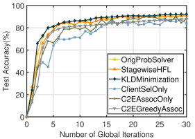
(a) MNIST

(b) CIFAR-10

Figure 2: Performance comparison in terms of test accuracy.

Fig. 2 shows the performance in terms of test accuracy on MNIST and CIFAR-10, where $\mathcal{T}$ and $\mathcal{L}$ are set to 5 and 3, respectively[10, 49]. As shown in Fig. 2(a), our StagewiseHFL outperforms ClientSelOnly, C2EAssocOnly and C2EGreedyAssoc by achieving higher test accuracy by 3.12%, 7.11%, and 3.03%, respectively, within 30 global iterations on MNIST. Comparing to OrigProbSolver, our StagewiseHFL obtains a slightly lower test accuracy (around 0.34% lower). This is because our proposed Plan A relies heavily on historical information, where the gap between the estimation from historical records and the actual network condition (i.e., actual attendance of clients) can lead to performance degradation. We will later show that this slight performance edge of OrigProbSolver comes with the drawback of significant running-time, rendering it inapplicable for large scale systems (later depicted in Fig. 5). Similarly, our StagewiseHFL exhibits 1.31% lower test accuracy than KLDMinimization method. This is because KLDMinimization solely focuses achieving data homogeneity (i.e., IID data) across the ESs, while ignoring the cost (i.e., latency and energy consumption) induced by such C2E assignment. As a result, as later shown, KLDMinimization suffers from a prohibitively high cost $F$ and running time. The high performance of OrigProbSolver, KLDMinimization, and our StagewiseHFL, particularly in terms of test accuracy and convergence speed, underscores a key insight: as the distribution of data across ESs becomes more uniform, the convergence of the model can be greatly improved reflected by the reduction of the number of global rounds required to reach the target accuracy). This phenomenon highlights the effectiveness of our method in optimizing the learning process by ensuring a more balanced data distribution across the ESs, enhancing the efficiency of HFL.

Similarly, considering CIFAR-10, our StagewiseHFL outperforms ClientSelOnly, C2EAssocOnly and C2EGreedyAssoc on CIFAR-10 by 6.12%, 5.52%, and 6.25% in test accuracy, while being only 0.71% lower than OrigProbSolver and 2.33% lower than KLDMinimization after 100 global iterations, as shown in Fig. 2(b). We next show that our method, while showing slightly lower prediction performance than the best benchmark, exhibits a notable performance gap when other metrics are considered.

5.1.2 Evaluation of delay, energy cost, and running time

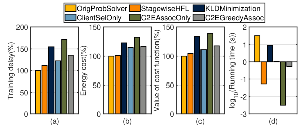
Figure 3: Performance on training delay, energy consumption, overall cost, and running time upon having real-world dataset

Fig. 3 illustrates the training delay, energy consumption, the overall cost (i.e., $\sum_{g}{F^{(g)}}$), and the time consumed for inference decision, to reach over 90% test accuracy on MNIST. We set $\mathcal{T}=5$, $\mathcal{L}=3$, and regard OrigProbSolver as the reference line, to better show the gap among different methods in Figs. 3(a)-3(d). In Fig. 3(a), the weighting factors $\lambda_{t}$ (for delay) and $\lambda_{e}$ (for energy) are assigned values of 1 and 0, respectively. This indicates that we put full emphasis on minimizing the training delay. Comparing to OrigProbSolver method which optimizes problem $\bm{\mathcal{P}}^{(g)}_{0}$ at the beginning of each global iteration, different benchmark methods can introduce various levels of increase on the training delay due to the complications embedded in their mechanism designs: 11.6%, 54.8%, 22.2%, 70.8%, and 35.4% increase for StagewiseHFL, KLDMinimization, ClientSelOnly, C2EAssocOnly, and C2EGreedyAssoc, respectively. StagewiseHFL stands out as the superior choice among the evaluated methods. In Fig. 3(b), we showcase the performance metrics related to energy consumption, by setting $\lambda_{t}=0$ and $\lambda_{e}=1$. Our StagewiseHFL, in comparison to OrigProbSolver, incurs only a marginal performance loss of 1.0%. This slight decrease demonstrates StagewiseHFL’s superior efficiency, highlighting its capability in balancing energy conservation and performance. Without loss of generality, when it comes to randomly assigning weighting factors of training delay and energy consumption such that $\lambda_{t}+\lambda_{e}=1$ ($\lambda_{t}$, $\lambda_{e}\in\left(0,1\right)$) in Fig. 3(c), our StagewiseHFL only incurs a 4.7% loss compared to OrigProbSolver, while achieving performance improvements of up to 28.5%, 22.1%, 34.2%, and 22.1%, in comparison with KLDMinimization, ClientSelOnly, C2EAssocOnly and C2EGreedyAssoc, respectively. We next show that the above-discussed close performance of our method to the best baseline comes with a notable gap in terms of running time.

To illustrate the online decision-making overhead of different methods, i.e., the time spent on selecting clients and associating them with ESs, Fig. 3(d) employs a logarithmic scale to represent the average decision-making time per global training round. Our StagewiseHFL shows the closest performance to OrigProbSolver in terms of cost savings (see Figs. 3(a)-3(c)), while offering an average inference time of less than 100ms, which is order of magnitude lower than that of OrigProbSolver. This shows the effectiveness of our approach in terms of achieving a reasonable value of resource consumption (i.e., energy and delay) under a notably low decision-making overhead.

5.2 Numerical Data-driven Experiments

To further evaluate our approach’s decision-making overhead and model convergence, we conduct a complementary set of experiments. These experiments aim to investigate the impact of various factors, such as the number of clients (i.e., $|\mathcal{N}|$) and ESs (i.e., $|\mathcal{S}|$), the minimum acceptable data size for model training (i.e., $D_{\textrm{min}}$), and the likelihood of client participation (i.e., $p_{i}$), on the performance.

TABLE II: Parameter setting used in Sec. 5.2
* $\mathcal{I}_{1}$: [0.4, 1), $\mathcal{I}_{2}$: [0.45, 1), $\mathcal{I}_{3}$: [0.5, 1), $\mathcal{I}_{4}$: [0.6, 1), $\mathcal{I}_{5}$: [0.7, 1)

	$|\mathcal{N}|$	$|\mathcal{S}|$	$D_{\textrm{min}}$	$p_{i}$
Set#1	75, 80, $\ldots$, 120	4	2500	$\mathcal{I}_{2}$
Set#2	100	3, 4, $\ldots$,7	2500	$\mathcal{I}_{2}$
Set#3	100	4	2000, 2500, $\ldots$, 4000	$\mathcal{I}_{2}$
Set#4	100	4	2500	$\mathcal{I}_{1}$, $\mathcal{I}_{2}$, $\ldots$, $\mathcal{I}_{5}$

5.2.1 Evaluation of the overall cost

We first evaluate the induced cost to achieve a 90% accuracy on MNIST dataset under various parameters: the number of clients $|\mathcal{N}|$, the number of ESs $|\mathcal{S}|$, the tolerable minimum data size $D_{\textrm{min}}$ for each ES, and the participation probability $p_{i}$ for each client $\bm{n}_{i}$. For illustrations, we conduct the next experiments under 4 sets of parameters detailed in Table 2.

We present a performance comparison on the value of cost function $F$ in Fig. 4(a), using OrigProbSolver as the reference line. Taking into account varying numbers of clients (75 to 120), our StagewiseHFL experiences a performance gap of 7.6%, 3.3%, 7.1%, 6.2%, and 7.2% as compared to OrigProbSolver. The is because Plan A in StagewiseHFL relies on historical data, introducing risks of inaccurate estimates in client selection and C2E association (the drawbacks associated with running time of OrigProbSolver will be analyzed in Fig. 5). Our StagewiseHFL exhibits cost-effectiveness when $|\mathcal{N}|$ ranges from 75 to 120 compared to KLDMinimization, ClientSelOnly, C2EAssocOnly and C2EGreedyAssoc. This is attributed to our optimized decision-making process for both client selection and C2E association. For instance, upon having $|\mathcal{N}|=80$ in Fig. 4(a), StagewiseHFL achieves a reduction in system cost by 7.7%, 10.26%, 19.5% and 22.2% as compared to KLDMinimization, ClientSelOnly, C2EAssocOnly and C2EGreedyAssoc, respectively. A similar trend, where our StagewiseHFL demonstrates cost-saving performance that ranks second with a small margin only to OrigProbSolver, is seen in Figs. 4(b)-4(d).

(a) Cost v.s. $|\mathcal{N}|$ (Set#1)

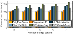
(b) Cost v.s. $|\mathcal{S}|$ (Set#2)

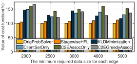
(c) Cost v.s. $D_{\textrm{min}}$ (Set#3)

(d) Cost v.s. $p_{i}$ (Set#4)

Figure 4: Performance on the overall system cost within numerical dataset.

(a) Running time v.s. $|\mathcal{N}|$ (Set#1)

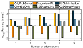
(b) Running time v.s. $|\mathcal{S}|$ (Set#2)

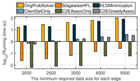
(c) Running time v.s. $D_{\textrm{min}}$ (Set#3)

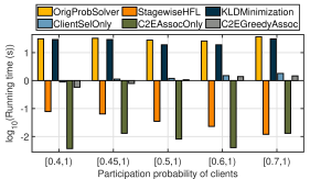
(d) Running time v.s. $p_{i}$ (Set#4)

Figure 5: Performance on running time within numerical dataset.

5.2.2 Evaluation of running time

Fig. 5 shows time efficiency reflected by running time, upon having different values of $|\mathcal{N}|$, $|\mathcal{S}|$, $D_{\textrm{min}}$, and $p_{i}$. Our StagewiseHFL significantly improves time efficiency compared to the benchmark methods under consideration, with the exception of C2EAssocOnly in some certain scenarios. This is because C2EAssocOnly does not prioritize optimizing client selection, thereby streamlining the decision-making process (however, it suffers from a large cost shown in Fig. 4).

Inspecting Figs. 5(a)-5(c), varying $|\mathcal{N}|$, $|\mathcal{S}|$ and $D_{\textrm{min}}$ changes the problem scale, which in turn affects the complexity of algorithms used for client selection and C2E association. For instance, in Fig. 5(a), the delay on decision-making of ClientSelOnly increases from 600ms to 9.8s with $|\mathcal{N}|$ rises from 70 to 120. Note that although OrigprobSolver outperforms our StagewiseHFL in terms of cost savings (see Fig. 4), its inference delay becomes prohibitively high as the problem size increases (with the rise of $|\mathcal{N}|$, $|\mathcal{S}|$ and $D_{\textrm{min}}$). For example, its decision-making delay varies from 10.44s to 346s as $|\mathcal{S}|$ increases from 3 to 7, shown in Fig. 5(b). While the time cost does escalate with an increase in problem size, our approach continues to be viable across various environments compared to all benchmarks. This superior performance is primarily due to our strategically designed Plan A, which pre-selects a specific number of long-term clients. This significantly mitigates the problem size encountered in Plan B, thereby accelerating the online decision-making process for client selection and C2E associations. A similar trend is found in Fig. 5(c), where rising tolerable minimum data size $D_{\textrm{min}}$ results in a growth of inference time, e.g., the inference time increases from 22s to 80s for KLDMinimization while from 24ms to 260ms for our StagewiseHFL when $D_{\textrm{min}}$ varies from 2000 to 5000. Also, as the client participation probability rises, our StagewiseHFL increasingly relies less on Plan B during actual training (since more selected long-term clients will participate in training), resulting in reduced complexity and further enhancing inference speeds. As illustrated in Fig. 5(d), having the client online probability range of [0.7, 1), StagewiseHFL achieves an average of only 12ms per global aggregation round, which is even faster than C2EAssocOnly.

In summary, Fig. 5 reveals that the running time of StagewiseHFL consistently remains below 500ms across various problem scales, which offers a commendable reference for future low-overhead HFL design in dynamic environments.

5.3 Analysis of the Impact of Key Parameters

Since improper parameter settings can adversely affect system performance, we further evaluate various combinations of ${\it{KLD}}_{\textrm{max}}$ and $D_{\textrm{min}}$, as well as $\mathcal{T}$ and $\mathcal{L}$ in this section, to show how they affect the system while identifying the optimal combinations.

5.3.1 Analysis of the impact of risk-related parameters

Our StagewiseHFL introduces distinctive considerations on risk evaluation in Plan A, representing one of our contributions, which sets this work apart from existing studies. As two key parameters that affect the risks are KLD and data size, we first illustrates how ${\it{KLD}}_{\textrm{max}}$ and $D_{\textrm{min}}$ impact the overall system cost and the required global aggregation rounds to reach a target test accuracy in Table 3. To achieve 90% accuracy on MNIST within $\mathcal{T}=5$ and $\mathcal{L}=3$, Table 3 shows that lowering the KLD for edge data can reduce the number of global aggregations. Considering $D_{\textrm{min}}=2500$, setting the value of ${\it{KLD}}_{\textrm{max}}$ from 0.5 to 0.2 reduces global iterations from 29 to 19. However, under non-IID data, setting the value of ${\it{KLD}}_{\textrm{max}}$ too low often leads to the selection of more clients for participation, increasing system costs. For example, when ${\it{KLD}}_{\textrm{max}}=0.1$, the system costs are higher than those with ${\it{KLD}}_{\textrm{max}}=0.2$ for all $D_{\textrm{min}}$ settings. For the tolerable data size, although raising $D_{\textrm{min}}$ can help improve model accuracy, when $D_{\textrm{min}}$ is set to a higher value, incorporating an excessive amount of data into training may decelerate convergence, thereby necessitating an increased number of global aggregations. For instance, upon having ${\it{KLD}}_{\textrm{max}}=0.4$, increasing $D_{\textrm{min}}$ from 2000 to 4000 increases the required global aggregation rounds from 27 to 36. In sum, the careful selection of $D_{\textrm{min}}$ and ${\it{KLD}}_{\textrm{max}}$ is crucial for optimizing the overall performance.

TABLE III: Impact of $D_{\textrm{min}}$ v.s. ${\it{KLD}}_{\textrm{max}}$ for reaching the accuracy of 90%

Cost/		${\it{KLD}}_{\textrm{max}}$
Aggregations		0.1	0.2	0.3	0.4	0.5
	2000	18.09/23	11.02/23	9.65/22	11.29/27	11.89/28
	2500	17.31/22	9.11/19	10.91/26	13.15/29	13.18/29
	3000	16.53/21	10.09/20	14.18/30	17.48/35	21.75/47
	4000	17.37/22	14.08/24	11.80/22	18.79/36	20.00/36
$D_{\textrm{min}}$	5000	16.58/21	14.75/22	14.36/23	14.73/23	15.52/25

5.3.2 Analysis of the impact of training configuration

We next analyze the impact of $\mathcal{T}$ and $\mathcal{L}$ on the overall system cost. Although $\mathcal{T}$ and $\mathcal{L}$ could ideally be optimized alongside other parameters to minimize overall system costs, our experiments are conducted under constraints including server access limitations $M_{j}$ and fixed data volumes. As a result, the number of clients selected in each global iteration remains relatively consistent, enabling us to identify a practical and broadly applicable combination of $\mathcal{T}$ and $\mathcal{L}$. This outcome aligns with existing works [5, 8, 10, 49], which similarly adopt certain fixed settings to keep the problem tractable.

As shown in Table 4, when $\mathcal{T}$ is relatively small (e.g., $\mathcal{T}=5$ and $\mathcal{L}=10$), increasing the value of $\mathcal{L}$ can effectively decrease the number of required global iterations, thereby enhancing the model’s convergence speed. At a specific intermediate value (e.g., $\mathcal{L}=3$), we achieve a joint minimum for both the system cost and the required number of global aggregations. However, with larger values of $\mathcal{T}$, the number of global aggregations needed for achieving the target accuracy may not necessarily reduce; in fact, it could result in inferior performance outcomes. Due to the imbalanced data distribution across clients and a lower edge aggregation frequency (that is, executing more local iterations within a single round of edge iteration), the local models may become biased, preventing the global model from convergence. Particularly if $\mathcal{L}=4$ and $\mathcal{L}=5$ when $\mathcal{T}=50$, the global model never reaches the accuracy of 90% and thus the training cost is denoted by infinity.

5.4 Threats to Validity

Since this work is the first attempt to having two complementary client recruitment plans, this section is dedicated to studying the validity of StagewiseHFL through inspecting factors that can compromise its effectiveness. Our goal is to highlight our method’s benefits from a rational perspective.

5.4.1 Threats to internal validity

The first threat to the our method’s validity is that the experimental environment may have favored our StagewiseHFL in the previous results. To fairly compare the performance of different methods, we change the settings of different parameters, e.g., $D_{\textrm{min}}$, and $p_{i}$, while we also perform 100 experiments for diverse parameter settings (Table 2). Note that when clients have a high online probability, e.g., an extreme case in which all the clients will join in each global training rounds ($p_{i}=1$, $\forall\bm{n}_{i}\in\mathcal{N}$), our design of pre-selection and pre-association of clients in Plan A may be no longer needed. The reason is that our plan A may result in a high overlap in the selected long-term clients, during each global iteration, potentially decreasing the diversity of training data while slowing down the convergence speed of the global model. As shown in Fig. 6(a), when the interval of $p_{i}$ varies from [0.75, 1) to [0.95, 1), our StagewiseHFL incurs performance losses of 26.5%, 39.4%, 33.6%, 23.2%, 28.0% compared to OrigprobSolver in terms of cost-savings. It may also perform worse in comparison with C2EGreedyAssoc, and even worse than the ClientSelOnly and KLDMinimization in some cases. Such observations indicate that our StagewiseHFL should be used in scenarios with intermittent client participation.

TABLE IV: Impact of $\mathcal{T}$ v.s. $\mathcal{L}$ for reaching the accuracy of 90%

Cost/		$\mathcal{L}$
Aggregations		1	2	3	4	5
	5	10.32/52	11.06/28	9.11/19	12.58/16	15.69/16
	10	12.03/41	13.45/23	14.21/16	18.90/16	16.23/11
	20	13.86/28	15.83/16	16.30/11	21.70/11	27.11/11
	30	31.16/23	15.25/11	22.83/11	30.41/11	37.99/11
$\mathcal{T}$	50	17.46/16	23.95/11	35.88/11	$\infty$	$\infty$

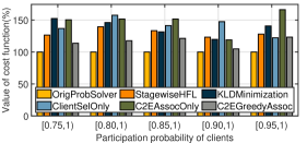
(a) Cost v.s. $p_{i}$

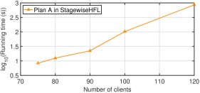
(b) Running time v.s. $|\mathcal{N}|$ for Plan A in StagewiseHFL

Figure 6: Invalidity of StagewiseHFL.

5.4.2 Threats to external validity

We next focus on the fact that the scale of network can impact the applicability of the offline decision-making portion our method. According to the discussions in Sec. 4.2.1, the computational complexity of Plan A can be impacted by the number of clients $|\mathcal{N}|$, which can lead to an excessively long decision-making time upon having a large $|\mathcal{N}|$. As illustrated by Fig. 6(b), when the value of $|\mathcal{N}|$ rises from 75 to 120, the time consumed by decision-making in Plan A increases from 8.3s to 855.8s, which implies that as the problem scale raises, our StagewiseHFL requires sacrificing a certain amount of offline decision-making time for a smooth training process. Nevertheless, since Plan A is activated just once prior to the model training (with the time spent on additional adjustments to the pre-decisions not included in the real-time decision-making time), such increases in decision-making are not of paramount concern as long as they are in tolerable ranges depending on the scenario of interest.

6 Conclusion and Future Work

In this paper, we studied client selection and C2E association for dynamic HFL network, for which we investigate a stagewise decision-making methodology with two stages, namely Plan A and Plan B. In particular, in Plan A, we introduced the concept of “continuity” of clients, strategically determining long-term clients and associating them with appropriate ESs. In Plan B, we propose a method for rapidly identifying backup clients in case those recruited by Plan A were unavailable in practical model training rounds. Comprehensive simulations on MNIST and CIFAR-10 datasets demonstrated the commendable performance of our method compared to other benchmark methods. Future avenues of research include the integration of uncertainties in clients local computation and communication capabilities into the system model. Also, exploring device-to-device (D2D) communications to enhance the local model aggregations under intermittent client availability is an enticing direction. We aim for this work to be the first in the literature to unveil the feasibility of stage-wise decision-making for FL and HFL, and to demonstrate the significant acceleration in FL and HFL execution that such decision-making can offer. Furthermore, we expect that the promising results and the intuitive logic of this approach will inspire future independent studies focused on the optimality analysis of stage-wise decision-making methods for FL.

Appendix A List of Notations

TABLE V: List of Notations

Notation	Definition	Notation	Definition
$\mathcal{N}$/$\bm{n}_{i}$	Set of clients/the $i^{\text{th}}$ client	$\mathcal{S}$/$s_{j}$	Set of ESs/the $j^{\text{th}}$ ES
$\mathcal{Z}$/$z_{h}$	Label set/the $h^{\text{th}}$ label	$\mathcal{D}_{i}$	Dataset of client $\bm{n}_{i}$
$d_{i}^{(g)}$	Data size of client $\bm{n}_{i}$	$D_{j}^{(g)}$	Data size of all clients associated with ES $s_{j}$
$D^{(g)}$	Data size of all clients that take part in the training process	$\boldsymbol{x}_{k}$/${y}_{k}$	Input vector/labeled output of the $k^{\text{th}}$ data
${v}_{i}$	CPU frequency of client $\bm{n}_{i}$	${q}_{i}$	Transmission power of client $\bm{n}_{i}$
$\xi_{i}^{(g)}$	Binary indicator describing the participation of a client $\bm{n}_{i}$ in $g^{\text{th}}$ global iteration	$\boldsymbol{A}^{(g)}$	Association matrix indicating whether client $\bm{n}_{i}$ is associated with ES $s_{j}$ or not
$\boldsymbol{\omega}_{i}^{(g;\ell,t)}$	Local model parameter of client $\bm{n}_{i}$ in $t^{\text{th}}$ local update during $\ell^{\text{th}}$ edge aggregation round	$\boldsymbol{\omega}_{j}^{(g;\ell)}$	Edge model parameter of ES $s_{j}$ in $\ell^{\text{th}}$ edge aggregation round
$\boldsymbol{\omega}^{(g)}$	Global model parameter	$\eta$	Learning rate
$\mathcal{T}$/$\mathcal{L}$	Edge/global aggregation frequency	$c_{i}$	Number of CPU cycles required for processing one sample data on $\bm{n}_{i}$
$\alpha_{i}$	Effective capacitance coefficient of $\bm{n}_{i}$’s computing chipset	$B_{j}$	Allocated bandwidth for each client associated with $s_{j}$
$M_{j}$	Maximum number of clients that can access to $s_{j}$	$h_{i,j}^{(g)}$	Channel gain of between $\bm{n}_{i}$ and $s_{j}$
$N_{0}$	Noise power spectral density	$R_{i,j}^{(g)}$	Data transmission rate of the uplink from client $\bm{n}_{i}$ to ES $s_{j}$
$\Omega$	Data size of the model parameters uploaded by clients	$p_{i}$	Participation probability of $\bm{n}_{i}$
$t_{i}^{\textrm{cmp}}$/$e_{i}^{\textrm{cmp}}$	Computation latency/energy consumption for a client $\bm{n}_{i}$ to perform one local training iteration	$t_{i,j}^{(g),\textrm{com}}$/$e_{i,j}^{(g),\textrm{com}}$	Transmission delay/energy consumption between $\bm{n}_{i}$ and $s_{j}$ during one edge iteration
$T_{i,j}^{(g)}$/$E_{i,j}^{(g)}$	Delay/energy consumption caused by the interaction between $\bm{n}_{i}$ and $s_{j}$ during one edge iteration	$T_{j}^{(g),\textrm{com}}$/$E_{j}^{(g),\textrm{com}}$	Transmission delay/energy consumption for ES $s_{j}$ uploading the edge model to the CS
$\mathbb{T}^{(g)}$/$\mathbb{E}^{(g)}$	Overall training delay/energy consumption during $g^{\text{th}}$ global iteration	$\mathbb{C}^{(g)}$	System “continuity” describing the geometric mean of online probability of each selected client
$\boldsymbol{y}_{i}$	Vector representing the data distribution of client $\bm{n}_{i}$	$\boldsymbol{P}_{j}^{(g)}$/$\boldsymbol{Q}$	Data distribution of ES $s_{j}$/reference data distribution
${\it{KLD}}_{\textrm{max}}$	Upper bound of KLD the covered data associated with each ES	$D_{\textrm{min}}$	lower bound of size of the covered data associated with each ES

Appendix B Derivation of (12)

By substituting the definition of $\operatorname{KLD}\left(\widehat{\boldsymbol{P}}_{j}^{(g)}||\boldsymbol{Q}\right)$ from (7) and (8) into (11a), we can obtain

$$\operatorname{Pr}\left(\sum_{h=1}^{|\mathcal{Z}|}\frac{\sum_{i=1}^{|\mathcal{N}|}\widehat{a}_{i,j}^{(g)}\xi_{i}^{(g)}\boldsymbol{y}_{i}(h)}{\sum_{i=1}^{|\mathcal{N}|}\widehat{a}_{i,j}^{(g)}\xi_{i}^{(g)}d_{i}}\operatorname{log}\frac{\sum_{i=1}^{|\mathcal{N}|}\widehat{a}_{i,j}^{(g)}\xi_{i}^{(g)}\boldsymbol{y}_{i}(h)}{\boldsymbol{Q}(h)\widehat{a}_{i,j}^{(g)}\xi_{i}^{(g)}d_{i}}>{\it{KLD}}_{\textrm{max}}-\Delta_{k}\right)\leq\delta,\forall s_{j}\in\mathcal{S}.$$ (13)

Note that the fractions in the above (13) have no meaning when $\sum_{i=1}^{|\mathcal{N}|}\widehat{a}_{i,j}^{(g)}\xi_{i}^{(g)}=0$, i.e., all clients selected and associated with ES $s_{j}$ in plan A are offline, then we consider $\operatorname{KLD}\left(\widehat{\boldsymbol{P}}_{j}^{(g)}||\boldsymbol{Q}\right)$ to be $+\infty$ in such a case. Given the law of total probability, we can decompose the left side of (11a) as:

$$\operatorname{Pr}\!\left(\operatorname{KLD}\left(\widehat{\boldsymbol{P}}_{j}^{(g)}||\boldsymbol{Q}\right)\!>\!{\it{KLD}}_{\textrm{max}}\!-\!\Delta_{k}\right)\!=\!\operatorname{Pr}\left(\sum_{i=1}^{|\mathcal{N}|}\widehat{a}_{i,j}^{(g)}\xi_{i}^{(g)}\!=\!0\right)\!\times\!\operatorname{Pr}\!\left(\operatorname{KLD}\left(\widehat{\boldsymbol{P}}_{j}^{(g)}||\boldsymbol{Q}\right)\!>\!{\it{KLD}}_{\textrm{max}}\!-\!\Delta_{k}\Big{|}\sum_{i=1}^{|\mathcal{N}|}\widehat{a}_{i,j}^{(g)}\xi_{i}^{(g)}\!=\!0\right)$$

$$+\operatorname{Pr}\left(\sum_{i=1}^{|\mathcal{N}|}\widehat{a}_{i,j}^{(g)}\xi_{i}^{(g)}\neq 0\right)\times\operatorname{Pr}\left(\operatorname{KLD}\left(\widehat{\boldsymbol{P}}_{j}^{(g)}||\boldsymbol{Q}\right)>{\it{KLD}}_{\textrm{max}}-\Delta_{k}\Big{|}\sum_{i=1}^{|\mathcal{N}|}\widehat{a}_{i,j}^{(g)}\xi_{i}^{(g)}\neq 0\right)$$

$$=\!\prod_{i\mid\widehat{a}_{i,j}^{(g)}=1}\!{\left(1-p_{i}\right)}+\left(1-\!\prod_{i\mid\widehat{a}_{i,j}^{(g)}=1}{\left(1-p_{i}\right)}\right)\!\times\operatorname{Pr}\left(\sum_{h=1}^{|\mathcal{Z}|}\frac{\sum_{i=1}^{|\mathcal{N}|}\widehat{a}_{i,j}^{(g)}\xi_{i}^{(g)}\boldsymbol{y}_{i}(h)}{\sum_{i=1}^{|\mathcal{N}|}\widehat{a}_{i,j}^{(g)}\xi_{i}^{(g)}d_{i}}\operatorname{log}\frac{\sum_{i=1}^{|\mathcal{N}|}\widehat{a}_{i,j}^{(g)}\xi_{i}^{(g)}\boldsymbol{y}_{i}(h)}{\boldsymbol{Q}(h)\widehat{a}_{i,j}^{(g)}\xi_{i}^{(g)}d_{i}}\Big{|}\sum_{i=1}^{|\mathcal{N}|}\widehat{a}_{i,j}^{(g)}\xi_{i}^{(g)}\neq 0\right).\!\!$$ (14)

For the case where $\sum_{i=1}^{|\mathcal{N}|}\widehat{a}_{i,j}^{(g)}\xi_{i}^{(g)}\neq 0$, let $\bm{R}_{j}^{(g)}(h)=\dfrac{\sum_{i=1}^{|\mathcal{N}|}\widehat{a}_{i,j}^{(g)}\xi_{i}^{(g)}\boldsymbol{y}_{i}(h)}{\sum_{i=1}^{|\mathcal{N}|}\widehat{a}_{i,j}^{(g)}\xi_{i}^{(g)}d_{i}}$, and define $N_{j}^{(g)}=\sum_{i=1}^{|\mathcal{N}|}\widehat{a}_{i,j}^{(g)}$ as the number of clients associated with ES $s_{j}$. Then, we have the following scenarios.

When $N_{j}^{(g)}=1$, we have $\bm{R}_{j}^{(g)}(h)=\dfrac{\bm{y}_{1}(h)\xi_{1}^{(g)}}{d_{1}\xi_{1}^{(g)}}=\dfrac{\bm{y}_{1}(h)}{d_{1}}.$

When $N_{j}^{(g)}=2$, we have $\bm{R}_{j}^{(g)}(h)=\dfrac{\bm{y}_{1}(h)\xi^{(g)}_{1}+\bm{y}_{2}(h)\xi^{(g)}_{2}}{d_{1}\xi^{(g)}_{1}+d_{2}\xi^{(g)}_{2}}=\dfrac{\bm{y}_{1}(h)\xi^{(g)}_{1}+\bm{y}_{1}(h)\dfrac{d_{2}}{d_{1}}\xi^{(g)}_{2}}{d_{1}\xi^{(g)}_{1}+d_{2}\xi^{(g)}_{2}}+\dfrac{\left(\bm{y}_{2}(h)-\bm{y}_{1}(h)\dfrac{d_{2}}{d_{1}}\right)\xi^{(g)}_{2}}{d_{1}\xi^{(g)}_{1}+d_{2}\xi^{(g)}_{2}}=\dfrac{\bm{y}_{1}(h)}{d_{1}}+\dfrac{d_{2}\left(\dfrac{\bm{y}_{2}(h)}{d_{2}}-\dfrac{\bm{y}_{1}(h)}{d_{1}}\right)\xi^{(g)}_{2}}{d_{1}\xi^{(g)}_{1}+d_{2}\xi^{(g)}_{2}}.$

When $N_{j}^{(g)}=3$, we have $\bm{R}_{j}^{(g)}(h)=\dfrac{\bm{y}_{1}(h)\xi^{(g)}_{1}+\bm{y}_{2}(h)\xi^{(g)}_{2}+\bm{y}_{3}(h)\xi^{(g)}_{3}}{d_{1}\xi^{(g)}_{1}+d_{2}\xi^{(g)}_{2}+d_{3}\xi^{(g)}_{3}}=\dfrac{\bm{y}_{1}(h)\xi^{(g)}_{1}+\bm{y}_{1}(h)\dfrac{d_{2}}{d_{1}}\xi^{(g)}_{2}+\bm{y}_{1}(h)\dfrac{d_{3}}{d_{1}}\xi^{(g)}_{3}}{d_{1}\xi^{(g)}_{1}+d_{2}\xi^{(g)}_{2}+d_{3}\xi^{(g)}_{3}}+\dfrac{\left(\bm{y}_{2}(h)-\bm{y}_{1}(h)\dfrac{d_{2}}{d_{1}}\right)\xi^{(g)}_{2}}{d_{1}\xi^{(g)}_{1}+d_{2}\xi^{(g)}_{2}+d_{3}\xi^{(g)}_{3}}+\dfrac{\left(\bm{y}_{3}(h)-\bm{y}_{1}(h)\dfrac{d_{3}}{d_{1}}\right)\xi^{(g)}_{3}}{d_{1}\xi^{(g)}_{1}+d_{2}\xi^{(g)}_{2}+d_{3}\xi^{(g)}_{3}}=\dfrac{\bm{y}_{1}(h)}{d_{1}}+\dfrac{d_{2}\left(\dfrac{\bm{y}_{2}(h)}{d_{2}}-\dfrac{\bm{y}_{1}(h)}{d_{1}}\right)\xi^{(g)}_{2}}{d_{1}\xi^{(g)}_{1}+d_{2}\xi^{(g)}_{2}+d_{3}\xi^{(g)}_{3}}+\dfrac{d_{3}\left(\dfrac{\bm{y}_{3}(h)}{d_{3}}-\dfrac{\bm{y}_{1}(h)}{d_{1}}\right)\xi^{(g)}_{3}}{d_{1}\xi^{(g)}_{1}+d_{3}\xi^{(g)}_{2}+d_{3}\xi^{(g)}_{3}}.$

Therefore, when $N_{j}^{(g)}$ takes a general positive integer, we can get

$$\bm{R}_{j}^{(g)}(h) =\dfrac{\bm{y}_{1}(h)\xi^{(g)}_{1}+\bm{y}_{2}(h)\xi^{(g)}_{2}+\ldots+\bm{y}_{N_{j}^{(g)}}(h)\xi^{(g)}_{N_{j}^{(g)}}}{d_{1}\xi^{(g)}_{1}+d_{2}\xi^{(g)}_{2}+\ldots+d_{N_{j}^{(g)}}\xi^{(g)}_{N_{j}^{(g)}}}=\dfrac{\bm{y}_{1}(h)}{d_{1}}+\dfrac{d_{2}\left(\dfrac{\bm{y}_{2}(h)}{d_{2}}-\dfrac{\bm{y}_{1}(h)}{d_{1}}\right)\xi^{(g)}_{2}}{d_{1}\xi^{(g)}_{1}+d_{2}\xi^{(g)}_{2}+\ldots+d_{N_{j}^{(g)}}\xi^{(g)}_{N_{j}^{(g)}}}$$

$$+\ldots+\dfrac{d_{N_{j}^{(g)}}\left(\dfrac{\bm{y}_{N_{j}^{(g)}}(h)}{d_{N_{j}^{(g)}}}-\dfrac{\bm{y}_{1}(h)}{d_{1}}\right)\xi^{(g)}_{N_{j}^{(g)}}}{d_{1}\xi^{(g)}_{1}+d_{2}\xi^{(g)}_{2}+\ldots+d_{N_{j}^{(g)}}\xi^{(g)}_{N_{j}^{(g)}}}.$$ (15)

Note that when $\dfrac{\bm{y}_{1}(h)}{d_{1}}=\underset{i\mid\widehat{a}_{i,j}^{(g)}=1}{\max}\left\{\dfrac{\bm{y}_{i}(h)}{d_{i}}\right\}$, all but the first term $\dfrac{\bm{y}_{1}(h)}{d_{1}}$ in the above equation are less than 0, i.e., $\bm{R}_{j}^{(g)}(h)=\dfrac{\bm{y}_{1}(h)}{d_{1}}+\dfrac{d_{2}\left(\dfrac{\bm{y}_{2}(h)}{d_{2}}-\dfrac{\bm{y}_{1}(h)}{d_{1}}\right)\xi^{(g)}_{2}}{d_{1}\xi^{(g)}_{1}+d_{2}\xi^{(g)}_{2}+\ldots+d_{N_{j}^{(g)}}\xi^{(g)}_{N_{j}^{(g)}}}+\ldots+\dfrac{d_{N_{j}^{(g)}}\left(\dfrac{\bm{y}_{N_{j}^{(g)}}(h)}{d_{N_{j}^{(g)}}}-\dfrac{\bm{y}_{1}(h)}{d_{1}}\right)\xi^{(g)}_{N_{j}^{(g)}}}{d_{1}\xi^{(g)}_{1}+d_{2}\xi^{(g)}_{2}+\ldots+d_{N_{j}^{(g)}}\xi^{(g)}_{N_{j}^{(g)}}}\leq\dfrac{\bm{y}_{1}(h)}{d_{1}}$. Similarly, when $\dfrac{\bm{y}_{1}(h)}{d_{1}}=\underset{i\mid\widehat{a}_{i,j}^{(g)}=1}{\min}\left\{\dfrac{\bm{y}_{i}(h)}{d_{i}}\right\}$, $\bm{R}_{j}^{(g)}(h)=\dfrac{\bm{y}_{1}(h)}{d_{1}}+\dfrac{d_{2}\left(\dfrac{\bm{y}_{2}(h)}{d_{2}}-\dfrac{\bm{y}_{1}(h)}{d_{1}}\right)\xi^{(g)}_{2}}{d_{1}\xi^{(g)}_{1}+d_{2}\xi^{(g)}_{2}+\ldots+d_{N_{j}^{(g)}}\xi^{(g)}_{N_{j}^{(g)}}}+\ldots+\dfrac{d_{N_{j}^{(g)}}\left(\dfrac{\bm{y}_{N_{j}^{(g)}}(h)}{d_{N_{j}^{(g)}}}-\dfrac{\bm{y}_{1}(h)}{d_{1}}\right)\xi^{(g)}_{N_{j}^{(g)}}}{d_{1}\xi^{(g)}_{1}+d_{2}\xi^{(g)}_{2}+\ldots+d_{N_{j}^{(g)}}\xi^{(g)}_{N_{j}^{(g)}}}\geq\dfrac{\bm{y}_{1}(h)}{d_{1}}$.

Accordingly, we can easily derive that $\underset{i\mid\widehat{a}_{i,j}^{(g)}=1}{\min}\left\{\dfrac{\bm{y}_{i}(h)}{d_{i}}\right\}\leq\bm{R}_{j}^{(g)}(h)\leq\underset{i\mid\widehat{a}_{i,j}^{(g)}=1}{\max}\left\{\dfrac{\bm{y}_{i}(h)}{d_{i}}\right\}$.

To facilitate the analysis, we construct a function $\operatorname{U}\left(\cdot\right)$ on $\bm{R}_{j}^{(g)}(h)$ such that $\operatorname{U}\left(\bm{R}_{j}^{(g)}(h)\right)=\bm{R}_{j}^{(g)}(h)\operatorname{log}\left(\dfrac{\bm{R}_{j}^{(g)}(h)}{\bm{Q}(h)}\right)$. This function is evidently convex in the domain $(0,+\infty)$, and it attains a local minimum at $\bm{R}_{j}^{(g)}(h)=\dfrac{\bm{Q}(h)}{e}$. Based on the relationship between the local minimum point $\dfrac{\bm{Q}(h)}{e}$ and the values of $\underset{i\mid\widehat{a}_{i,j}^{(g)}=1}{\min}\left\{\dfrac{\bm{y}_{i}(h)}{d_{i}}\right\}$ and $\underset{i\mid\widehat{a}_{i,j}^{(g)}=1}{\max}\left\{\dfrac{\bm{y}_{i}(h)}{d_{i}}\right\}$, we can determine the upper bound of $\operatorname{U}\left(\bm{R}_{j}^{(g)}(h)\right)$ when $\bm{R}_{j}^{(g)}(h)$ lies in $\left[\underset{i\mid\widehat{a}_{i,j}^{(g)}=1}{\min}\left\{\dfrac{\bm{y}_{i}(h)}{d_{i}}\right\},\underset{i\mid\widehat{a}_{i,j}^{(g)}=1}{\max}\left\{\dfrac{\bm{y}_{i}(h)}{d_{i}}\right\}\right]$.

Specially, it can be categorized into the following three cases: i) when $\dfrac{\bm{Q}(h)}{e}\geq\underset{i\mid\widehat{a}_{i,j}^{(g)}=1}{\max}\left\{\dfrac{\bm{y}_{i}(h)}{d_{i}}\right\}$, we have $\operatorname{U}\left(\bm{R}_{j}^{(g)}(h)\right)\leq\operatorname{U}\left(\underset{i\mid\widehat{a}_{i,j}^{(g)}=1}{\min}\left\{\dfrac{\bm{y}_{i}(h)}{d_{i}}\right\}\right)$; ii) when $\dfrac{\bm{Q}(h)}{e}\leq\underset{i\mid\widehat{a}_{i,j}^{(g)}=1}{\min}\left\{\dfrac{\bm{y}_{i}(h)}{d_{i}}\right\}$, we have $\operatorname{U}\left(\bm{R}_{j}^{(g)}(h)\right)\leq\operatorname{U}\left(\underset{i\mid\widehat{a}_{i,j}^{(g)}=1}{\max}\left\{\dfrac{\bm{y}_{i}(h)}{d_{i}}\right\}\right)$; iii) when $\underset{i\mid\widehat{a}_{i,j}^{(g)}=1}{\min}\left\{\dfrac{\bm{y}_{i}(h)}{d_{i}}\right\}\leq\dfrac{\bm{Q}(h)}{e}\leq\underset{i\mid\widehat{a}_{i,j}^{(g)}=1}{\max}\left\{\dfrac{\bm{y}_{i}(h)}{d_{i}}\right\}$, we have $\operatorname{U}\left(\bm{R}_{j}^{(g)}(h)\right)\leq\max{\left\{\operatorname{U}\left(\underset{i\mid\widehat{a}_{i,j}^{(g)}=1}{\min}\left\{\dfrac{\bm{y}_{i}(h)}{d_{i}}\right\}\right),\operatorname{U}\left(\underset{i\mid\widehat{a}_{i,j}^{(g)}=1}{\max}\left\{\dfrac{\bm{y}_{i}(h)}{d_{i}}\right\}\right)\right\}}$.

Let us define a function

$$\bm{G}_{j}^{(g)}(h)=\begin{cases}\operatorname{U}\left(\underset{i\mid\widehat{a}_{i,j}^{(g)}=1}{\min}\left\{\dfrac{\bm{y}_{i}(h)}{d_{i}}\right\}\right)&,\dfrac{\bm{Q}(h)}{e}\geq\underset{i\mid\widehat{a}_{i,j}^{(g)}=1}{\max}\left\{\dfrac{\bm{y}_{i}(h)}{d_{i}}\right\}\\ \operatorname{U}\left(\underset{i\mid\widehat{a}_{i,j}^{(g)}=1}{\max}\left\{\dfrac{\bm{y}_{i}(h)}{d_{i}}\right\}\right)&,\dfrac{\bm{Q}(h)}{e}\leq\underset{i\mid\widehat{a}_{i,j}^{(g)}=1}{\min}\left\{\dfrac{\bm{y}_{i}(h)}{d_{i}}\right\}\\ \max{\left\{\operatorname{U}\left(\underset{i\mid\widehat{a}_{i,j}^{(g)}=1}{\min}\left\{\dfrac{\bm{y}_{i}(h)}{d_{i}}\right\}\right),\operatorname{U}\left(\underset{i\mid\widehat{a}_{i,j}^{(g)}=1}{\max}\left\{\dfrac{\bm{y}_{i}(h)}{d_{i}}\right\}\right)\right\}}&,{\text{otherwize.}}\end{cases}$$ (16)

as the upper bound of $\operatorname{U}\left(\bm{R}_{j}^{(g)}(h)\right)$. We can then obtain the upper bound of $\operatorname{Pr}\left(\operatorname{KLD}\left(\widehat{\boldsymbol{P}}_{j}^{(g)}||\boldsymbol{Q}\right)>{\it{KLD}}_{\textrm{max}}-\Delta_{k}\mid\sum_{i=1}^{|\mathcal{N}|}\widehat{a}_{i,j}^{(g)}\xi_{i}^{(g)}\neq 0\right)$ according to the Markov inequality as follows:

$$\operatorname{Pr}\left(\operatorname{KLD}\left(\widehat{\boldsymbol{P}}_{j}^{(g)}||\boldsymbol{Q}\right)>{\it{KLD}}_{\textrm{max}}-\Delta_{k}\Big{|}\sum_{i=1}^{|\mathcal{N}|}\widehat{a}_{i,j}^{(g)}\xi_{i}^{(g)}\neq 0\right)\leq\dfrac{\mathbf{E}\left[\sum_{h=1}^{|\mathcal{Z}|}\operatorname{U}\left(\bm{R}_{j}^{(g)}(h)\right)\Big{|}\sum_{i=1}^{|\mathcal{N}|}\widehat{a}_{i,j}^{(g)}\xi_{i}^{(g)}\neq 0\right]}{{\it{KLD}}_{\textrm{max}}-\Delta_{k}})$$

$$=\sum_{h=1}^{|\mathcal{Z}|}\dfrac{\mathbf{E}\left[\operatorname{U}\left(\bm{R}_{j}^{(g)}(h)\right)\Big{|}\sum_{i=1}^{|\mathcal{N}|}\widehat{a}_{i,j}^{(g)}\xi_{i}^{(g)}\neq 0\right]}{{\it{KLD}}_{\textrm{max}}-\Delta_{k}}\leq\sum_{h=1}^{|\mathcal{Z}|}\dfrac{\bm{G}_{j}^{(g)}(h)}{{\it{KLD}}_{\textrm{max}}-\Delta_{k}},$$ (17)

where $\mathbf{E}\left[\cdot\right]$ is the expectation operator. Finally, we can get the upper bound of $\operatorname{Pr}\left(\operatorname{KLD}\left(\widehat{\boldsymbol{P}}_{j}^{(g)}||\boldsymbol{Q}\right)>{\it{KLD}}_{\textrm{max}}-\Delta_{k}\right)$ as follows:

$$\operatorname{Pr}\left(\operatorname{KLD}\left(\widehat{\boldsymbol{P}}_{j}^{(g)}||\boldsymbol{Q}\right)>{\it{KLD}}_{\textrm{max}}-\Delta_{k}\right)=\!\prod_{i\mid\widehat{a}_{i,j}^{(g)}=1}{\left(1-p_{i}\right)}+\left(1-\!\prod_{i\mid\widehat{a}_{i,j}^{(g)}=1}\!{\left(1-p_{i}\right)}\right)$$

$$\times\!\operatorname{Pr}\!\left(\operatorname{KLD}\left(\widehat{\boldsymbol{P}}_{j}^{(g)}||\boldsymbol{Q}\right)\!>\!{\it{KLD}}_{\textrm{max}}\!-\!\Delta_{k}\Big{|}\sum_{i=1}^{|\mathcal{N}|}\widehat{a}_{i,j}^{(g)}\xi_{i}^{(g)}\neq 0\right)\!\leq\!\!\prod_{i\mid\widehat{a}_{i,j}^{(g)}=1}\!\!{\left(1-\!p_{i}\right)}\!\left(1-\!\!\prod_{i\mid\widehat{a}_{i,j}^{(g)}=1}\!\!{\left(1-\!p_{i}\right)}\!\right)\!\times\!\sum_{h=1}^{|\mathcal{Z}|}\!\dfrac{\bm{G}_{j}^{(g)}(h)}{{\it{KLD}}_{\textrm{max}}\!-\!\Delta_{k}}.\!\!\!$$ (18)

Therefore, the constraint (11a) is tightened to (12) in Sec. 4.2.1, which is

$$\prod_{i\mid a_{i,j}^{\prime}=1}\left(1-p_{i}\right)+\left(1-\prod_{i\mid a_{i,j}^{\prime}=1}\left(1-p_{i}\right)\right)\times\sum_{h=1}^{|\bm{\mathcal{Z}}|}\frac{\bm{G}_{j}^{(g)}(h)}{{\it{KLD}}_{\textrm{max}}-\Delta_{k}}\leq\delta,\forall s_{j}\in\mathcal{S}.$$

Appendix C Derivation of (11g)

By substituting the definition of $D_{j}^{(g)}$ into the above (11b), we can obtain that

$$\operatorname{Pr}\left(\sum_{i=1}^{|\mathcal{N}|}\widehat{a}_{i,j}^{(g)}\xi_{i}^{(g)}d_{i}<D_{\textrm{min}}+\Delta_{d}\right)\leq\varepsilon,\forall s_{j}\in\mathcal{S}.$$ (19)

Base on the Markov inequality, we can obtain the lower bound of the left side of the above inequality as follows:

$$\operatorname{Pr}\left(\sum_{i=1}^{|\mathcal{N}|}\widehat{a}_{i,j}^{(g)}\xi_{i}^{(g)}d_{i}<D_{\textrm{min}}+\Delta_{d}\right)\geq 1-\frac{\mathbf{E}\left[\sum_{i=1}^{|\mathcal{N}|}\widehat{a}_{i,j}^{(g)}\xi_{i}^{(g)}d_{i}\right]}{D_{\textrm{min}}+\Delta_{d}},\forall s_{j}\in\mathcal{S}.$$ (20)

Further, according to the linearity of expectation, we can get

$$\mathbf{E}\left(\sum_{i=1}^{|\mathcal{N}|}\widehat{a}_{i,j}^{(g)}\xi_{i}^{(g)}d_{i}\right)=\sum_{i=1}^{|\mathcal{N}|}\widehat{a}_{i,j}^{(g)}\mathbf{E}\left(\xi_{i}^{(g)}\right)d_{i}=\sum_{i=1}^{|\mathcal{N}|}\widehat{a}_{i,j}^{(g)}p_{i}d_{i},\forall s_{j}\in\mathcal{S}.$$ (21)

We can thus relax the constraint (11b) to

$$1-\frac{\sum_{i=1}^{|\mathcal{N}|}\widehat{a}_{i,j}^{(g)}p_{i}d_{i}}{D_{\textrm{min}}+\Delta_{d}}\leq\varepsilon,\forall s_{j}\in\mathcal{S},$$ (22)

which results in (11g):

$$\sum_{i=1}^{|\mathcal{N}|}\widehat{a}_{i,j}^{(g)}p_{i}d_{i}\geq\left(D_{\textrm{min}}+\Delta_{d}\right)\left(1-\varepsilon\right),\forall s_{j}\in\mathcal{S}.$$

Appendix D Additional experiment I

To simulate a more realistic dynamic scenario, we set the channel gain between clients and ESs to fluctuate within the range of $[10^{-9},10^{-8}]$, and their CPU frequencies fluctuate within the range of $[1,10]$ for each global iteration (in contrast to the fixed values used in Section V). Moreover, since both the channel conditions and client computing capabilities vary, we need to execute an additional Plan A to ensure the accurate estimation of the clients’ online probability. Therefore, we simply set the frequency of Plan A execution to once per 10 rounds, to adapt to the varies in environmental parameters in the dynamic scenario.

Fig. 7 illustrates the training delay, energy consumption, overall cost, and the time consumed for inference decision-making to achieve over 90% test accuracy on MNIST. Compared to Fig. 3, in the dynamic scenario, our proposed StagewiseHFL still maintains excellent robustness. In terms of training delay, energy consumption, and overall cost, StagewiseHFL only incurs an increase of 13.2%, 3.0%, and 6.0%, respectively, compared to OrigProbSolver, still demonstrates better performance compared to other benchmark. In terms of inference latency, StagewiseHFL requires an average of only 51ms, demonstrating its superior effectiveness and efficiency in decision-making speed. This is because the additional execution of Plan A is performed in parallel with the training process, and therefore does not add extra real-time decision delay to the training progress.

Although we acknowledge the need for additional validation in highly dynamic environments, we can adjust the frequency at which Plan A is triggered to balance accurate optimization decisions against real-time decision efficiency. For instance, Plan A may be reactivated when:

$\bullet$ The system experiences unacceptable costs (e.g., excessive training delay or high energy consumption),

$\bullet$ Large changes are detected in channel conditions or clients’ computing capabilities, or

$\bullet$ A fixed number of global rounds has been completed.

Due to space limitation, we leave the exploration of these aspects to future work.

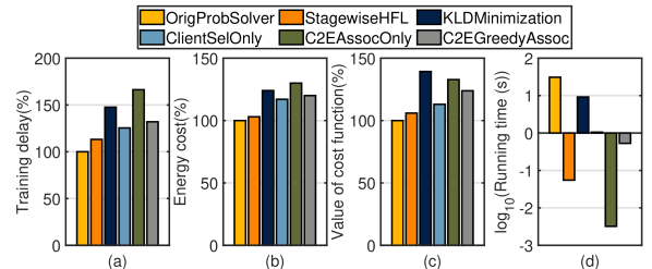
Figure 7: Performance on training delay, energy consumption, overall cost, and running time under varying channel conditions and clients’ computational capabilities.

Appendix E Additional experiment II

To verify the reliability of our handling of constraints (11a) and (11b) in Plan A, we performed simulations under various values of $D_{min}$ and ${\it{KLD}}_{\textrm{max}}$, evaluating the performance of StagewiseHFL in cost-saving and its approximation to OrigProbSolver. As shown in Fig. 8, in most experimental groups, the approximation is quite satisfactory. However, when the number of long-term clients determined in Plan A is large, the performance of StagewiseHFL decreases in terms of approximation to OrigProbSolver (for example, when $D_{\textrm{min}}=5000$ and ${\it{KLD}}_{\textrm{max}}=0.1$, the overall cost of StagewiseHFL is 11.6% and 9.59% higher than that of OrigProbSolver, respectively). This is due to the lack of diversity in the training data, which necessitates more global rounds to achieve the target accuracy, thus consuming more overall cost. Nevertheless, we typically adopt more appropriate settings for $D_{\textrm{min}}$ and ${\it{KLD}}_{\textrm{max}}$, and considering the reduced inference time overhead compared to StagewiseHFL, this performance still falls within an acceptable range.

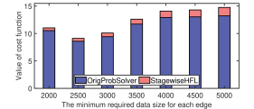
(a) Cost v.s. $D_{\textrm{min}}$

(b) Cost v.s. ${\it{KLD}}_{\textrm{max}}$

Figure 8: Performance on the overall system cost for OrigProbSolver and StagewiseHFL.

References

- [1] Z. Zhao et al., “DeepThings: distributed adaptive deep learning inference on resource-constrained IoT edge clusters”, IEEE Trans. Comput. Aided Des. Integr. Circuits Syst, vol. 37, no. 11, pp. 2348-2359, 2018.
- [2] B. McMahan et al., “Communication-efficient learning of deep networks from decentralized data,” Proc. Int. Conf. Artif. Intell. Stat., pp. 1273–1282, 2017.
- [3] Y. Zhou et al., “The role of communication time in the convergence of federated edge learning,” IEEE Trans. Veh. Technol., vol. 71, no. 3, pp. 3241–3254, 2022.
- [4] D. C. Nguyen et al., “Federated learning for internet of things: A comprehensive survey,” IEEE Commun. Surveys Tut., vol. 23, no. 3, pp. 1622-1658, 2021.
- [5] S. Luo et al., “HFEL: Joint edge association and resource allocation for cost-efficient hierarchical federated edge learning,” IEEE Trans. Wireless Commun., vol. 19, no. 10, pp. 6535-6548, 2020.
- [6] Z. Jiang et al., “Computation and communication efficient federated learning with adaptive model pruning,” IEEE Trans. Mobile Comput., vol. 23, no. 3, pp. 2003-2021, 2024.
- [7] Y. Tian et al., “Hierarchical federated learning with adaptive clustering on Non-IID data,” Proc. IEEE Glob. Commun. Conf. (GLOBECOM), pp. 5063–5068, 2022
- [8] L. Liu et al., “Client-edge-cloud hierarchical federated learning,” IEEE Int. Conf. Commun. (ICC), pp. 1-6, 2020.
- [9] M. S. H. Abad et al., “Hierarchical federated learning across heterogeneous cellular networks,” IEEE Int. Conf. Acoust. Speech Signal Process Proc. (ICASSP), pp. 8866-8870, 2020.
- [10] Y. Deng et al., “A communication-efficient hierarchical federated learning framework via shaping data distribution at edge,” IEEE/ACM Trans. Netw., vol. 32, no. 3, pp. 2600-2615, 2024.
- [11] W. Mao et al., “Joint client selection and bandwidth allocation of wireless federated learning by deep reinforcement learning,” IEEE Trans. Serv. Comput., vol. 17, no. 1, pp. 336-348, 2024.
- [12] S. Fu et al., “Joint optimization of device selection and resource allocation for multiple federations in federated edge learning,” IEEE Trans. Serv. Comput., vol. 17, no. 1, pp. 251-262, 2024.
- [13] K. Bonawitz et al., “Practical secure aggregation for privacy-preserving machine learning,” Proc. ACM SIGSAC Conf. Comput. Commun. Secur. (CCS), pp. 1175–1191, 2017.
- [14] H. Saadat et al., “RL-assisted energy-aware user-edge association for IoT-based hierarchical federated learning,” Int. Wireless. Commun. Mob. Comput. (IWCMC), pp. 548-553, 2022.
- [15] J. Konečný et al., “Federated learning: Strategies for improving communication efficiency,” arXiv preprint arXiv:1610.05492, 2017.
- [16] S. Caldas et al., “Expanding the reach of federated learning by reducing client resource requirements,” arXiv:812.07210, 2019.
- [17] D. Alistarh et al., “QSGD: Communication-efficient SGD via gradient quantization and encoding,” Adv. neural inf. proces. syst., pp. 1707–1718, 2017.
- [18] X. Zhang et al., “Vehicle selection and resource allocation for federated learning-assisted vehicular network”, IEEE Trans. Serv. Comput., vol. 23, no. 5, pp. 3817-3829, 2024.
- [19] J. Zheng, “Federated learning for online resource allocation in mobile edge computing: A deep reinforcement learning approach,” Proc. IEEE Wireless Commun. Netw. Conf. (WCNC), pp. 1-6, 2023.
- [20] Z. Yang et al., “Energy efficient federated learning over wireless communication networks,” IEEE Trans. Wireless Commun., vol. 20, no. 3, pp. 1935–1949, 2021.
- [21] W. Wu et al., “Accelerating federated learning over reliability-agnostic clients in mobile edge computing systems,” IEEE Trans. Parallel Distrib. Syst., vol. 32, no. 7, pp. 1539-1551, 2021.
- [22] K. Yang et al., “Federated learning via over-the-air computation,” IEEE Trans. Wireless Commun., vol. 19, no. 3, pp. 2022-2035, 2020.
- [23] T. D. Burd et al., “Processor design for portable systems”, J. Signal Process. Syst., vol. 13, no. 2–3, pp. 203–221, 1996.
- [24] J. Feng et al., “Min-max cost optimization for efficient hierarchical federated learning in wireless edge networks,” IEEE Trans. Parallel Distrib. Syst., vol. 33, no. 11, pp. 2687-2700, 2022.
- [25] F. P. -C. Lin et al., “Delay-aware hierarchical federated learning,” IEEE Trans. Cognit. Commun. Netw., vol. 10, no. 2, pp. 674-688, 2024.
- [26] L. Su et al., “Low-latency hierarchical federated learning in wireless edge networks,” IEEE Internet Things J., vol. 11, no. 4, pp. 6943-6960, 2024.
- [27] Z. Qu et al., “Context-aware online client selection for hierarchical federated learning,” IEEE Trans. Parallel Distrib. Syst., vol. 33, no. 12, pp. 4353-4367, 2022.
- [28] T.T.Vu et al., “Cell-free massive MIMO for wireless federated learning,” IEEE Trans. Wireless Commun., vol. 19, no. 10, pp. 6377-6392, 2020.
- [29] X. Xia et al., “Formulating cost-effective data distribution strategies online for edge cache systems,” IEEE Trans. Parallel Distrib. Syst., vol. 33, no. 12, pp. 4270–4281, 2022.
- [30] Y. Sun et al., “Uplink interference mitigation for OFDMA femtocell networks,” IEEE Trans. Wireless Commun., vol. 11, no. 2, pp. 614-625, 2012.
- [31] X. Cao et al., “Transmission power control for over-the-air federated averaging at network edge,” IEEE J. Sel. Areas Commun., vol. 40, no. 5, pp. 1571–1586, 2022.
- [32] D.-J. Han, “FedMes: Speeding up federated learning with multiple edge servers,” IEEE J. Sel. Areas Commun., vol. 39, no. 12, pp. 3870–3885, 2021.
- [33] Y. Jiao “Toward an automated auction framework for wireless federated learning services market,” IEEE Trans. Mobile Comput., vol. 20, no. 10, pp. 3034-3048, 2021.
- [34] D. Chen et al., “Matching-theory-based low-latency scheme for multitask federated learning in MEC networks,” IEEE Internet Things J., vol. 8, no. 14, pp. 11415-11426, 2021.
- [35] L. Wang et al., “Towards class imbalance in federated learning,” arXiv preprint arXiv:2008.06217, 2020.
- [36] M. Pal et al., “Facility location with nonuniform hard capacities,” Annu Symp Found Comput Sci Proc, pp. 329–338, 2001.
- [37] Z. Cheng et al., “Joint client selection and task assignment for multi-task federated learning in MEC networks,” Proc. IEEE Glob. Commun. Conf. (GLOBECOM), pp. 1–6, 2021.
- [38] M. Ester et al., “A density-based algorithm for discovering clusters in large spatial databases with noise,” Int. Conf. Knowl. Discov. Data Min., pp. 226–231, 1996.
- [39] Y. Lecun et al., “Gradient-based learning applied to document recognition,” Proc. IEEE, vol. 86, no. 11, pp. 2278–2324, 1998.
- [40] A. Krizhevsky, “Learning multiple layers of features from tiny images,” Tech. Rep., 2009.
- [41] A. Byerly et al., “No routing needed between capsules,” Neurocomputing, pp. 545-553, 2021.
- [42] A. Dosovitskiy et al., “An image is worth 16x16 words: Transformers for image recognition at scale,”arXiv preprint arXiv:2010.11929, 2020.
- [43] L. U. Khan et al., “Federated learning for edge networks: Resource optimization and incentive mechanism,” IEEE Commun. Mag., vol. 58,no. 10, pp. 88–93, 2020.
- [44] W. Feller, “Markov Chains,” An introduction to probability theory and its applications, vol. 1, 3rd ed., Wiley, 1968.
- [45] M. Perlmutter et al.,“Scattering Statistics of Generalized Spatial Poisson Point Processes,” IEEE Int. Conf. Acoust. Speech Signal Process. (ICASSP), pp. 5528-5532, 2022.
- [46] R. He et al., “Non-stationary mobile-to-mobile channel modeling using the Gauss-Markov mobility model,” Int. Conf. Wirel. Commun. Signal Process. (WCSP), pp. 1-6 2017.
- [47] H. Wang et al., “Optimizing Federated Learning on Non-IID Data with Reinforcement Learning,” Proc. IEEE Conf. Comput. Commun. (INFOCOM), pp. 1698-1707, 2020.
- [48] W. Sunet al., “Accelerating Convergence of Federated Learning in MEC With Dynamic Community,” IEEE Trans. Mobile Comput., vol. 23, no. 2, pp. 1769-1784, 2024.
- [49] Y. Deng et al., “SHARE: Shaping Data Distribution at Edge for Communication-Efficient Hierarchical Federated Learning,” IEEE Int. Conf. Distrib. Comput. Syst. (ICDCS), pp. 24-34, 2021.
- [50] Z. Xu et al., “Energy or Accuracy? Near-Optimal User Selection and Aggregator Placement for Federated Learning in MEC,” IEEE Trans. Mobile Comput., vol. 23, no. 3, pp. 2470-2485, 2024.
- [51] B. Luo et al., “Cost-Effective Federated Learning Design,” IEEE Conf. Comput. Commun., pp. 1-10, 2021.
- [52] H. T. Nguyen et al., “Fast-Convergent Federated Learning,” IEEE J. Sel. Areas Commun., vol. 39, no. 1, pp. 201-218, 2021.
- [53] H. Xiao et al., “Fashion-MNIST: A novel image dataset for benchmarking machine learning algorithms,” arXiv:1708.07747, 2017.
- [54] K. He et al., “Deep residual learning for image recognition,” Proc. IEEE Conf. Comput. Vis. Pattern Recognit.(CVPR), pp. 770–778, 2016.
- [55] D. Xue et al., “Cost-Aware Hierarchical Federated Learning via Over-the-Air Computing,” Proc. IEEE Glob. Commun. Conf. (GLOBECOM), pp. 4728-4733, 2022.
- [56] Y. Guo et al., “Hybrid local SGD for federated learning with heterogeneous communications,” Int. Conf. Learn. Represent.(ICLR), pp. 1-42, 2022.
- [57] T. Castiglia et al., “Multi-level local SGD: Distributed SGD for heterogeneous hierarchical networks,” Int. Conf. Learn. Represent.(ICLR), pp. 1-36, 2021.
- [58] Z. Zhang et al., “Scalable and low-latency federated learning with cooperative mobile edge networking,” IEEE Trans. Mobile Comput., vol. 23, no. 1, pp. 812–822, 2024.