Optimal response for stochastic differential equations by local kernel perturbations
Abstract.
We consider a random dynamical system on , whose dynamics is defined by a stochastic differential equation. The annealed transfer operator associated with such systems is a kernel operator. Given a set of feasible infinitesimal perturbations to this kernel, with support in a certain compact set, and a specified observable function , we study which infinitesimal perturbation in produces the greatest change in expectation of . We establish conditions under which the optimal perturbation uniquely exists and present a numerical method to approximate the optimal infinitesimal kernel perturbation. Finally, we numerically illustrate our findings with concrete examples.
Key words and phrases:
Stochastic differential equations, transfer operators, linear response1991 Mathematics Subject Classification:
Primary: 37H10, 37C30, Secondary: 37M05, 37N35, 49N45, 60H101. Introduction
The predictive understanding and the control of the statistical properties of a dynamical system is an important topic of study, with applications to many different fields, so is understanding the change in these statistical properties after changes in the initial dynamical system. The concept of statistical stability of a dynamical system relates to the statistical properties of typical orbits of a dynamical system, which are in turn encoded into its invariant or stationary measures, and to how these properties change when the system is perturbed. We say that the system exhibits a linear response to the perturbation when such a change is differentiable (see Theorem 24 for a formalization of this concept). In this case, the long-time average of a given observable changes smoothly during the perturbation.
The linear response for dynamical systems was first studied by Ruelle [36], and then was studied extensively for different classes of systems having some form of hyperbolicity (see [4] for a general survey).The linear response for stochastic differential equations was studied in [23] and [10], where general response results were established. In the context of discrete-time random systems, linear response results have been shown in [16], [3] and [2]. The study of linear response has great importance in the applications, in particular to climate sciences (see [29], [23]).
In the present article, we address a natural inverse problem related to linear response: The Optimal Response of a given observable. We consider a certain observable, defined on the phase space associated with our system and search for the optimal infinitesimal perturbation to apply to the system in order to maximize the observable’s expectation. The understanding of this problem also has evident importance in the applications, as it is a formalization of the natural question of “how to manage the system in a way such that its statistical properties change in a wanted direction”, hence an optimal control problem for the statistical properties of the system.
The optimal response problem for a fixed observable as described above was studied for the first time in [1], for finite-state Markov chains.
Then the case of dynamical systems whose transfer operators are kernel operators (including random dynamical systems that have additive noise) was considered in [2].
The case of one-dimensional deterministic expanding circle maps with deterministic perturbations was studied in [14].
The above articles also consider the problem of optimizing the spectral gap and hence the speed of mixing. In [18], an optimal response problem is considered where optimal coupling is studied in the context of mean-field coupled systems.
A problem strictly related to the optimal response is the ‘linear request problem’, which focuses on the search for a perturbation achieving a prescribed response direction [9, 20, 16, 30, 28].
All of these studies are in terms of understanding how a system can be modified to control the behavior of its statistical properties.
Stochastic differential equations and random dynamical systems are widely used as models of climate and fluid dynamics related phenomena. This strongly motivates the study of the optimal response for such systems. As mentioned above, the optimal response and the control of the statistical properties for discrete time random dynamical systems whose associated transfer operator is a kernel operator is studied in [2] and [16]. In these papers, the phase space considered was compact. Since the transfer operator associated with a stochastic differential equation is a kernel operator (see Theorem 1 for a precise statement and estimates on the regularity of the kernel). The results of these papers hence apply to the case of time discretizations of stochastic differential equations over compact spaces. The extension of these results to non-compact phase space is a non-trivial task, which requires the use of suitable functional spaces, in order to recover the “compact immersion”-like functional analytic properties, which are well known to be important to establish spectral gap for the associated transfer operator. Important stochastic differential models are formulated on noncompact spaces, such as . Thus, such an extension is strongly motivated. An approach to the definition of suitable spaces for the transfer operators associated with stochastic differential equations on was implemented in [13], by using a sort of weighted Bounded Variation spaces with the scope of studying extreme events.
In the present paper, motivated by these considerations, we approach the study of optimal linear response for random dynamical systems over that have a kernel transfer operator, and we suppose that this operator is the one coming from a Stochastic Differential Equation. This setting is, in our opinion, a first step in approaching the study of the optimal response for Stochastic Differential Equations.
Overview of the paper. We consider a discrete time random system on the phase space whose dynamics is defined by a stochastic differential equation (SDE) having Lipschitz regularity and which is dissipative, in the sense that its deterministic part is sending some large ball centered in the origin to itself (see (1) and the assumptions (2) and (3)).
We then consider the transfer operator associated with the system (see (6)). This operator is a kernel operator (see Theorem 1) on the non-compact phase space .
In subsection 3.2 we define suitable spaces for this operator.
We will let the transfer operator act on and on a “stronger” space, constructed using a space we denote by which is a space of densities which decay at infinity with a prescribed speed. The choice of the topology is motivated by optimization purposes, which are simplified when working on a Hilbert space. The prescribed decay at infinity will be useful in obtaining suitable compactness properties, which will imply that the transfer operator, when considered on the strong space, has a spectral gap (see Lemma 14) and strong mixing properties (see Proposition 17).
In Section 4 we define and study the perturbations we intend to apply to our system. The perturbations we consider (see (20)) are applied directly to the associated transfer operator, additively to its kernel on a compact domain of the phase space. 111We remark that the transfer operator that we obtain after perturbation, may not be the one associated with an SDE anymore. Such a perturbation can be interpreted as a ”local” change to the initial system (which is the one arising from an SDE) whose nature is independent from the phenomenon whose model is the SDE. Although this is a limitation in interpreting the present work as the study of the optimal response for SDE, we think the present work is a first step in this direction.
In the section we show that the perturbed operators too have spectral gap, and we prove a linear response statement for those systems and perturbations (see Theorem 24).
Finally, we consider an observable in and explore the problem of finding the optimal perturbation, which maximises the rate of change of expectation of the observable (see Section 5). We formalize (see Problem 26) the optimization problem and prove (see Proposition 27) that the problem has a unique solution.
In Section 5.2, we describe a numerical approach to approximate the unique solution in the case where the set of feasible perturbations is a ball in a suitable Hilbert space.
In Section 6 we apply the algorithm to illustrate the optimal perturbation on some examples. In particular, we consider a gradient system SDE with symmetric double-well potential. Then, via a finite difference method, we numerically approximate the solution of the optimization problem for a smooth observable given by the probability density function of a Gaussian random variable.
2. Recalling Stochastic Differential Equations
Consider a stochastic differential equation on of the following type
| (1) |
where is the Brownian motion defined on a probability space . We make following assumptions on the drift :
- A:
-
(Locally-Lipschitz continuity) For each , there is and such that for all with ,
(2) - B:
-
(Dissipativity) We assume that there exist constants with such that for all
(3)
If the system given by (1) satisfies the above assumptions A and B, then it has a unique stationary measure (see [13, Section 4.1]).
Now let , for be the flow solving the deterministic part of the above SDE, that is
Let and be the Gaussian distribution given by
The following key result from literature shows useful estimates on the densities of the solutions of the SDE (1):
Theorem 1 ([32], Theorem 1.2 and Remark 1.3.).
Fix . For each and let be the unique solution of (1) starting from at time . Then has a density which for each can be expressed as a function that is continuous in both variables. Moreover, satisfies the following:
- 1:
-
(Two sided density bounds) There exist depending on such that for any
- 2:
-
(Gradient estimates) There exist depending on such that for any
Remark 2.
As stated above, the SDE that we consider in this article has a unique stationary measure . In the following we fix the time and consider a time discretization of this system. In the notations thus drop the subscript . Hence, in the following, the kernel will be denoted as .
3. Transfer operator and Banach spaces
3.1. The Kolmogorov operator and the transfer operator
In this section, we define the transfer operator associated with the evolution of the SDE considered at time and state/prove some basic properties of these operators. We will extensively use the density (as Remark 2 says, we drop the subscript ) and its properties given by Theorem 1.
Definition 3.
The Kolmogorov operator associated with the system (1) at time is defined as follows. Let then
If is a Borel signed measure on
supposing that has a density with respect to the Lebesgue measure i.e we can thus write
| (5) |
Now we define the transfer operator associated with the evolution of the system at time .
Definition 4 (Transfer operator).
Given we define the measurable function as follows. For almost each let
| (6) |
Remark 5.
By (5) we now get the duality relation between the Kolmogorov and the transfer operator
| (7) |
The following are some well-known and basic facts about integral operators with
kernels in , which will be useful:
- •
-
•
If , then
(9) and the operator is bounded.
Now, we discuss the properties of the transfer operator on the space .
Lemma 6.
The operator preserves the integral and is a weak contraction with respect to the norm.
Proof.
Remark 7.
Since is a positive operator, we also get that is a Markov operator having kernel .
Finally, in the following section, we define/construct the strong space that we want to study the operator on.
3.2. Functional Spaces
We construct spaces suitable for our non-compact domains, that is the spaces consist of densities whose behavior far away from the origin is controlled using certain weight functions going to at infinity, following the approach of [13].
Let and define the weight function
| (10) |
Let be the space of Lebesgue measurable such that
Note that, and for , . Moreover for , .
Remark 8.
Throughout the article, we denote the and norms by and respectively.
For a Borel subset let us define
Let be a Radon probability measure on and assume that:
-
()
is absolutely continuous with respect to the Lebesgue measure, having a continuous bounded density such that everywhere.
With such a probability measure satisfying (), define a norm for by setting
| (11) |
where denotes the ball in with center and radius . Being the sum of a norm and a seminorm, indeed defines a norm and the following space is a Banach space222In [37] and [26], these spaces have been studied extensively and in more general form as well. (see [37, Proposition 3.3])
The presence of the measure in the definition of the oscillatory seminorm is necessary to treat the case when we have a non-compact domain, which in this case is . Instead, if the domain was compact, one could simply take .
Finally, to define the strong space, let be a compact set in . In what follows, is the set where we allow perturbations in our system. Accordingly, we define a suitable norm, adapted to such perturbations, as follows:
| (12) |
We define the strong space of densities as follows, equipped with the norm :
| (13) |
The following results from [13] will be useful to prove the compact inclusion of the strong space in and, ultimately, the spectral gap.
Proposition 9.
is a compact embedding.
Lemma 10.
There exist constants and such that
| (14) |
for every and every .
Lemma 11.
For every , is bounded linear from to ; in particular, there exists such that
| (15) |
Moreover if then
| (16) |
The proofs of Proposition 9, Lemma 10 and Lemma 11 can be found in [13, Theorem 16, Lemma 19 and Lemma 20] respectively.
Now we proceed to prove that the transfer operator has spectral gap when acting on , for which we need some preliminary results like compact inclusion (Proposition 12) and Lasota-Yorke inequality (Lemma 13) etc.
By Proposition 9, and Lemma 11 we have the following:
Proposition 12.
Let be the closed unit ball in . Then is a compact set in .
Proof.
Using Proposition 9, which states that is compactly embedded in , it suffices to prove that is a closed and bounded set in the space .
By Lemma 11, for every , there exists such that , which implies is a bounded set in .
To prove that is closed, let be a Cauchy sequence in . Since and is a Banach space, there exists such that . We want to show that . Since , there exists a sequence such that, for all , and . As the unit ball is closed, there exists such that . By continuity, we have , which implies , completing the proof.
∎
Lemma 13.
There exist constants and such that
| (17) |
for every and every .
Proof.
By Lemma 10, such that
Let us define the spaces of zero-average functions in and respectively as
| (18) |
and
| (19) |
In the rest of this section, we prove results on the functional analytic properties of the operator , namely, the existence of eigenvalues on the unit circle, the spectral gap, and the boundedness of the resolvent. These results, along with other inferences, give us the uniqueness of the invariant measure of the system in the strong space and its convergence to equilibrium. To prove these results, we extensively use the positivity of the kernel associated with the operator .
Lemma 14.
The transfer operator has spectral gap on and it has 1 as its simple and only eigenvalue on the unit circle.
Proof.
By Lemma 6, the operator is integral preserving, which implies that lies in the spectrum of .
Recall that, by Lemma 6 and Lemma 13, the operator satisfies the hypothesis of Hennion theorem (see [12, Theorem B.14]), which implies that the operator is quasi-compact which, in turn, implies that it has spectral gap on . Consequently, 1 is an eigenvalue of .
Now, we want to prove that 1 is the unique eigenvalue of on the unit circle. Let us suppose, to the contrary, that there exists an eigenvalue such that . Accordingly, there exists a corresponding eigenvector , that is
Then, for any ,
Since preserves the integral (Lemma 6), we have
This implies . Then, since the kernel is positive (by Theorem 1), we get
This contradicts the earlier calculation. Hence, 1 is the only eigenvalue of on the unit circle.
Now, to show that 1 is a simple eigenvalue, let be two distinct eigenvectors corresponding to the eigenvalue 1. Then
Since and are fixed points of , is also a fixed point of and hence an invariant measure. Notice that which implies . Again, since is positive, we have , which contradicts the fact that is a fixed point. Consequently, 1 is a simple eigenvalue of on . ∎
A first direct consequence of Lemma 14 is the uniqueness of the invariant probability measure of .
Proposition 15.
The operator has a unique invariant probability density . Hence satisfying and .
Remark 16.
We remark that the unique stationary measure of the SDE (1) must be also invariant for , and this must be the unique invariant probability measure found above. This also implies that has a density in the strong space (see Remark 2). We conclude that the unique stationary measure of the SDE is indeed equal to the invariant measure of the transfer operator.
The spectral gap and the uniqueness of the invariant probability measure for imply the following two classical consequences, which will be used later.
Proposition 17.
For each
and the resolvent operator is a bounded operator.
Proof.
By Lemma 14 and the fact that the operator is positive and integral preserving, we get that has spectral gap, which implies it can be decomposed as
where is the projection operator onto the one-dimensional eigenspace corresponding to the eigenvalue 1, and the spectral radius of is strictly less than 1, that is .
Furthermore, for we have , and
for some and . The first claim follows directly by this estimate. The second claim also follows from the estimate, since the resolvent operator can be written as . ∎
4. Perturbations and linear response
From now on, we denote the original transfer operator defined above by .
As mentioned in Section 1, to perturb the initial Stochastic differential equation (1) that we began with, we perturb the associated transfer operator (defined in Section 3). Since the transfer operator associated with a time discretisation of the system is a kernel operator (see Theorem 1 and (6)), we perturb the operator by perturbing the associated kernel. We would like to emphasise the fact that this method of perturbation has the limitation that the perturbed system may not correspond to a SDE. Rather, it signifies a “local” change in the initial SDE, whose nature is independent of the SDE model.
The local kernel perturbations are conducted in the following way:
let be a compact set, and let be given, then for every , define the family of kernels as
| (20) |
where with
Finally, define the linear operators (Hilbert-Schmidt integral operators) by
| (21) |
| (22) |
Let us assume that the operators are integral preserving for every , that is, for each
where is the Lebesgue measure.
Lemma 18.
For , the operator is integral preserving if and only if both and are zero average in in direction, that is, for almost each , .
Proof.
The converse part is straight forward, therefore we prove the forward implication. is integral preserving if and only if, for every
thus, the above equality reduces to , for every ,
Hence, for almost every ,
That is,
Taking limit both sides, we get
Since so is true for all , we get that for almost all , which implies .
∎
Now recall that by Proposition 15, there exists an invariant density (the eigenvector corresponding to the eigenvalue 1) of the operator . Consequently, we have the following lemma.
Lemma 19.
The operators and restricted to the strong space satisfy the following limit
where is the invariant density for the operator .
Proof.
The above lemma implies that the operator can be thought of as the derivative, with respect to , of the operator . Now, we are interested to consider the linear response of our systems to such perturbations. But first, let’s understand how close the perturbed operators are to the initial operator .
Lemma 20.
Let be a family of transfer operators associated with the kernels as before. Then, there exist constants such that for each
| (23) |
Proof.
Let be such that . Since is compactly supported on , it implies that is also compactly supported in D. Using the fact that inside the set , by Cauchy Schwartz inequality, the norms satisfy , for some , we have
where we have used that and in the last inequality we used (8). Since , there exists such that . Finally, using , we have the result. ∎
To obtain a result on linear response, we need the perturbed operators to possess certain properties, such as the Lasota-Yorke inequality, the existence of an invariant density, and a bounded resolvent. We prove these properties in the following lemmas.
Lemma 21.
Let be the family of transfer operators associated with the kernels as above. Then there exist constants , such that for each ,
| (24) |
Proof.
We have that
where in the last inequality we have used Holder’s inequality and the fact that and are supported only in . Now, using (8) and the fact that , there exists such that
| (25) |
Hence, there exists (depending on ) such that
By Theorem 13
Taking large enough, so that and so small such that , we get
Then, for every , we get
Similarly, for any , , proving a uniform Lasota-Yorke inequality for ∎
Proposition 22.
For the operators , and for small enough, there exists a unique invariant density with , that is, .
Proof.
Firstly, recall that for all , the operators are integral preserving, which implies 1 lies in the spectrum of . Indeed, consider the dual operators ; the fact that the operators are integral preserving implies that the Lebesgue measure is invariant for the dual operator . Accordingly, , that is, 1 is in the spectrum of the dual operators and hence in the spectrum of the operators for all .
Now, recall that by Lemma 14, 1 is the only eigenvalue of on the unit circle.
Observe that for every , the operator is a weak contraction on and satisfies Lasota-Yorke inequality (by Lemma 21). Further, using Lemma 20, and the fact that is compactly immersed inside (Lemma 12), we get, using [27, Theorem 1], that the isolated eigenvalues of are arbitrarily close to that of , that is, the leading eigenvalue of is also simple and satisfies that
which, in turn, implies that for small enough . Accordingly, there exists such that satisfying being a probability density. Note that such an invariant density is unique. Indeed, if there exists another invariant density , then note that , which implies
Accordingly, using (9),
Hence the uniqueness. ∎
To be able to state the linear response result, the last ingredient we need is the bounds on the resolvent of perturbed operators, and hence the following lemma. Recall the definition of and given by (18) and (19) respectively.
Lemma 23.
For small enough, the resolvent operators of the perturbed operators , given by , are well-defined and satisfy
and
Proof.
Finally, we can state a response result adapted to our kind of systems and perturbations.
Theorem 24.
For the operators , for small enough, we have linear response, that is
Though in this work we consider operators which are not necessarily positive, the proof of the above statement is similar to many other linear response results (see e.g. [14] Theorem 12, Appendix A). We include it for completeness.
Proof.
By Proposition 22, we know that for each , the operator has a fixed point . Accordingly, we get
By the preservation of integral, for each preserves . Since for all , and by Lemma 23, for small enough, is a uniformly bounded operator. Accordingly, we can apply the resolvent to both sides of the expression above to get
| (26) | ||||
| (27) |
Since, by Lemma 23, , we have
Further, Lemma 19 implies converges in then (26) implies that
∎
5. Optimisation of response
5.1. Optimization of the expectation of an observable
Consider the set of allowed infinitesimal perturbations (as described in Section 4) to the kernel . Fix an observable ; we are interested in finding, from the set of allowed perturbations, an optimal perturbation which maximises the rate of change of the expectation of . To perform the optimisation, we assume that is a bounded, closed and convex subset of the Hilbert space .
We believe that the above hypotheses on are natural; convexity is so because if two different perturbations of a system are possible, then their convex combination – applying the two perturbations with different intensities – should also be possible.
Let be an observable. If were the indicator function of a certain set, for example, one could control the invariant density towards the support of .
Given a family of kernels (as in Lemma 19) with associated transfer operators and invariant densities , we denote the response of the system to by
| (28) |
This limit converges in as proved in Theorem 24.
Lemma 25.
The operator defined in (28) is continuous.
Proof.
Using Theorem 24, we have
which implies
Thanks to Proposition 17, the operator is bounded, and thus is finite. Consider the following
Using Holder’s inequality and the fact that has compact support, we get
where is the same as given in (10). Finally, using (9) and again the fact that has compact support, there exists such that
The above calculation implies the operator is bounded and hence continuous. ∎
Under our assumptions, since , we easily get
| (29) |
Hence the rate of change of the expectation of with respect to is given by the linear response of the system under the given perturbation. To take advantage of the general results of Appendix A, we perform the optimisation of over the closed, bounded and convex subset of the Hilbert space containing the zero perturbation. To maximise the RHS of (29) we set
and consider the following problem:
Problem 26.
Find the solution to
| (30) | |||||
| (31) | subject to |
To answer the above problem, we state a rather general following result:
Proposition 27.
Let be a closed, bounded and strictly convex set such that its relative interior contains the zero vector. If is not uniformly vanishing on , then the problem
| (32) | |||||
| (33) | subject to |
has a unique solution.
Proof.
5.2. Numerical scheme for the approximation of the optimal perturbation
In this section, we present a simple numerical recipe to obtain a Fourier approximation of the optimal perturbation in Problem 26. Similar methods, based on Fourier approximation on suitable Hilbert spaces were used in [14], and [19].
By Lemma 25, and the fact that , we obtained in the proof of Proposition 27 that is continuous. Thus, being a Hilbert space, by using Riesz’s representation theorem, there exists such that
which implies that
Now we state how to approximate by computing its Fourier coefficients. Consider an orthonormal basis of444One can consider the basis consisting of indicator functions, or that of Hermite polynomials etc. and define
We have then that the sequence converges to as .
6. Numerical experiments
In this section, we present numerical experiments related to Problem 26.
We find the optimal infinitesimal perturbation that maximises the expected value of an observable, as discussed in Section 5.1. We will consider a suitable SDE on the real line and on this simple example we search for the optimal perturbation in order to maximize the increase of a certain observable.
Specifically, in Section 6.1 we present and describe the details of the gradient SDE that will express the dynamics of each of our experiments. Section 6.2 is aimed at describing a classical finite difference method used to solve the partial derivative equation of the parabolic type that identifies the solution law of the SDE. Section 6.3 presents how to numerically find the solution to the problem presented in Section 5.2. Finally, Section 6.4 presents and explains the results of our experiments. They consist of taking observables as probability density functions of Gaussian variables: symmetric with respect to the domain in the first case, and asymmetric in the second.
6.1. Gradient system and Fokker-Planck equation
We consider, for a noise intensity and a final time , the SDE given by
| (34) |
where is a symmetric double well potential. denotes a Brownian Motion (BM) and is a deterministic initial condition. The final time will be the time in which we investigate the optimal response in the following sections. In other words, we will numerically investigate the properties of the the transfer operator associated with the evolution of the SDE from time to time .
This SDE, which belongs to the class of gradient systems, is often used to describe bistability in many applications, such as phase separation in physics or abrupt climate shifts in paleoclimate studies. If , the dynamical system given by (34) presents three fixed points: and . The former are asymptotically stable and correspond to the minimum points of ; the latter is unstable, since it corresponds to a local maximum point of .
Considering the case , the existence and uniqueness of a solution is classical. Indeed, since the drift term is locally Lipschitz, the SDE (34) admits, locally in time, an almost everywhere (a.e.) continuous strong solution, see [6] for more details. Further, since the potential is coercive, finite time explosion of the solution can be ruled out ([31, Theorem 3.5]), resulting in the existence and uniqueness of a strong solution , for any . Furthermore, since the potential is regular and coercive, Hormander’s Theorem assures that the law of has a density with respect to the Lebesgue measure on , see [24] and [22, Section 7]. It satisfies, in the weak sense, the Fokker-Planck equation (FPE) ([35, 25, 21])
| (35) |
where is the drift term of the SDE (34) and denotes the Dirac delta concentrated in . Note that, given the final time , which is the same time at which we investigate the linear response, the kernel defining the transfer operator is given by
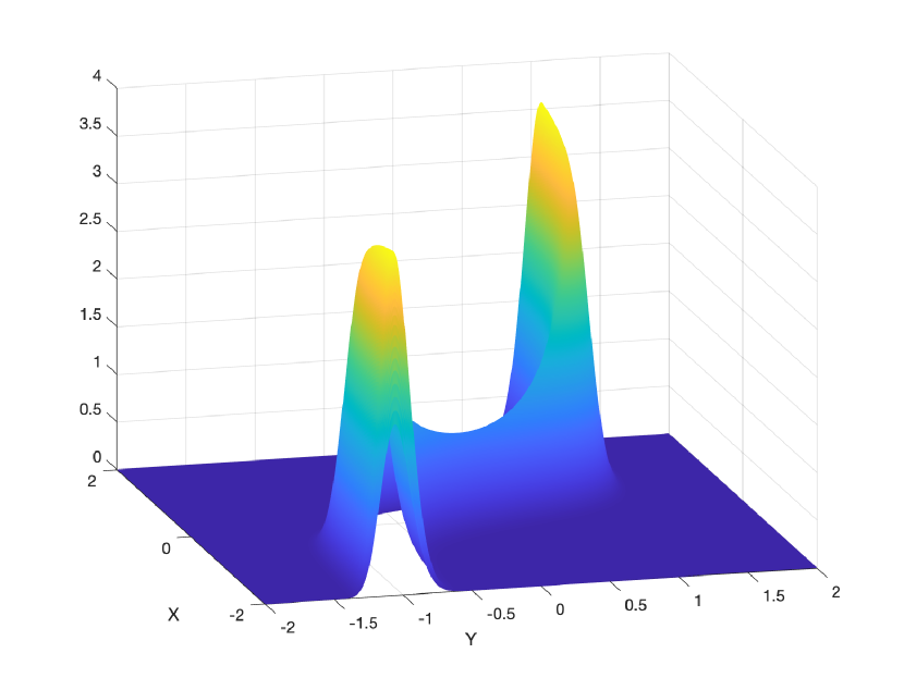
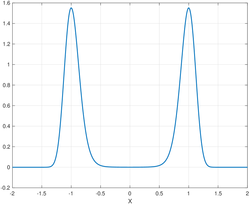
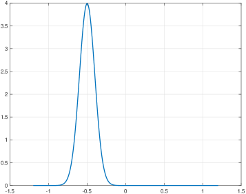
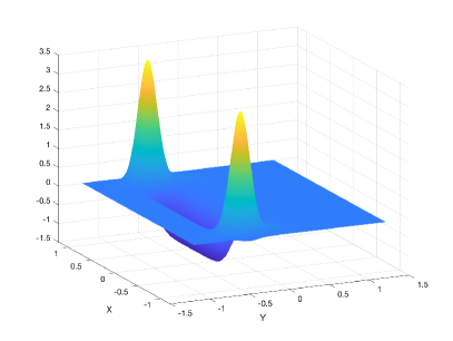
A numerical approximation of the kernel is represented in Figure 1(a), obtained for and . Given an initial condition , the probability density function (PDF) is concentrated around either or , depending on the sign of the initial condition. This bistability is clear also in Figure 1(b), which depicts the invariant density for . In fact, it is symmetric, with two maximum points in . In the next section, we are going to describe our numerical approximation for the solution of the FPE and how to use it to study the linear response problem.
6.2. Finite difference method for the Fokker-Planck equation
We apply an implicit finite-difference (FD) method ([34, 38]) to approximate the solution of the parabolic problem (35) in the finite domain , with the constraint to choose a sufficiently large such that , which describes a PDF, is negligible on . The FPE (35) is a second-order parabolic PDE, and to consider a solution, we need to complete it with boundary conditions at the end of the domain . We choose reflecting boundary conditions, which means that no probability mass can escape the domain ([21]). This leads to
| (36) |
First, we consider a uniform mesh of the space and time domain, i.e., we fix
and
where determine the number of points in the meshes. We denote by
the numerical approximation for the solution of (36). Similarly, we set
Second, we use the centered formula to approximate the second derivative, i.e.
and a centered difference for the first derivative
Note that in the previous equations, when we are at the boundary of , there appear the terms and . The former are just auxiliary unknowns, since the solution of the FPE is not defined outside ; the latter are defined as
In addition to this, to approximate the Dirac Delta we consider the same mesh for the initial condition domain, i.e., we set
Furthermore, for each we approximate the Dirac Delta with the PDF of a Gaussian random variable with mean and standard deviation .
In conclusion, for each , the implicit FD that we apply can be written as
| (37) |
6.3. Numerical scheme for the optimal response problem
In this section, we describe how to numerically approximate the solution of
| (38) |
where . We know that, given an observable , the optimal perturbation is given by
where denotes an orthonormal basis of and
Further, denotes the invariant density for . In particular, we consider as basis of the sine-cosine wavelets defined as
Note that we avoid inserting the wavelets with index in the basis defining the vector space of the allowed perturbation, since we impose that any perturbation needs to satisfy . Then, for each , we approximate the coefficient as follows.
Let and . We adopt the same notation for . First, the definite integral defining is approximated by using the composite Simpson’s rule ([33]), which leads to
| (39) |
with
Second, the vector is the solution of the linear system
The matrix represents the numerical approximation, via the same Simpson rule recalled before, of the operator . Its elements are given by
Further, the constant term vector is obtained by approximating the innermost integral of as follows
with and
Third, the invariant density is obtained by computing the left eigenvector corresponding to the eigenvalue of the matrix
where the entries of the matrix are given by
Indeed, this is equivalent to find a vector such that
Note that the left-hand side is an approximation of the transfer operator evaluated on . In fact, the previous equation, component-wise, reads as
with the left side being an approximation of . The existence of a such eigenvector for the eigenvalue is a consequence of the Perron-Frobenius Theorem for row stochastic matrices, see [7].
Lastly, the sum defining is truncated, and we consider the approximation of given by the elements in the truncated basis defined as
Thus, our approximation of the solution is given by
6.4. Results
In this section, we present our numerical experiments to approximate the solution of the optimal control problem (38) using two different observables, . Both observables are selected from the class of PDFs of Gaussian random variables with mean and variance .
In the first experiment, we use a symmetric observable with and . In the second experiment, we use an asymmetric observable with and . Similar results can be achieved by varying , , and the class of the observable (such as continuous bump functions or polynomials). However, using non-continuous observables (like indicator functions) may introduce minor numerical errors due to the finite selection of basis elements. We will discuss the results of the symmetric experiment, shown in Figure 2, in detail. The results for the asymmetric case, shown in Figure 3, follow the same explanation and are not repeated here.
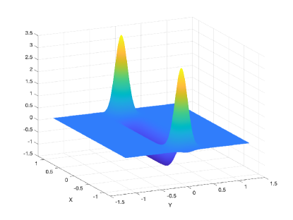
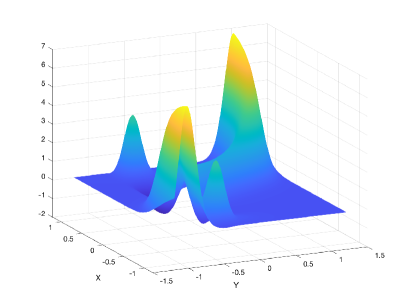
First, Figure 2(a) depicts the symmetric observable used in the first experiment. Figure 2(b) represents the approximation of the optimal perturbation that solves the problem (38). This optimal perturbation, , provides the infinitesimal adjustment to the kernel needed to maximize . It is worth pointing out that the perturbation is significant (i.e., far from zero) only where the observable is significant. Furthermore, for any given value where is significant, for example, , the restriction of the perturbation redistributes mass from areas where the invariant density is small (away from ) to areas where the invariant density is large (around ). Additionally, due to the choice of basis , it can be numerically verified that for any .
Figure 2(c) visually represents the perturbed kernel with and .
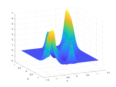
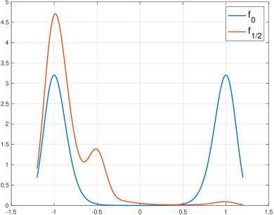
Lastly, Figure 2(d) compares the invariant densities and for the transfer operators and , respectively. These two symmetric densities, both normalized to satisfy , weight the points in differently. Specifically, is concentrated around , whereas , while preserving the same maximum points as , also shows a third local maximum at , where the observable is concentrated.


Code availability
All material in the text and figures was produced by the authors using standard mathematical and numerical analysis tools. The only externally supplied code of this work consists of the implementation of the Simpson’s rule for numerical integration by Damien Garcia (link), which we acknowledge.
The code for the numerical simulations performed in Section 6 is available at Zenodo (https://doi.org/10.5281/zenodo.13820212).555The code available on Zenodo performs the numerical experiments described in this work using and . To reproduce the results of this work, i.e., with , the reader should modify the number of points in the spatial mesh at line 16 of the code.
Appendix A Recap of convex optimisation
Let be a bounded and convex subset of a Hilbert space .
Definition 28.
We say that a convex closed set is strictly convex if for each pair and for all , the points , where is the relative interior666The relative interior of a closed convex set is the interior of relative to the closed affine hull of . of .
Let us briefly recall some relevant results from convex optimisation.
Suppose is a separable Hilbert space and . Let be a continuous linear
function. Consider the abstract problem to find such that
| (40) |
The existence and uniqueness of an optimal perturbation follows from properties of as stated in the following two propositions.
Proposition 29 (Existence of the optimal solution).
Let be bounded, convex, and closed in . Then problem (40) has at least one solution.
Upgrading convexity of the feasible set to strict convexity provides uniqueness of the optimal solution.
Proposition 30 (Uniqueness of the optimal solution).
Suppose is closed, bounded, and strictly convex subset of , and that contains the zero vector in its relative interior. If is not uniformly vanishing on
then the optimal solution to (40) is unique.
References
- [1] Fadi Antown, Davor Dragičević, and Gary Froyland. Optimal linear responses for markov chains and stochastically perturbed dynamical systems. Journal of Statistical Physics, 170:1051–1087, 3 2018.
- [2] Fadi Antown, Gary Froyland, and Stefano Galatolo. Optimal linear response for markov hilbert–schmidt integral operators and stochastic dynamical systems. Journal of Nonlinear Science, 32(79):60, 2022.
- [3] Wael Bahsoun, Marks Ruziboev, and Benoît Saussol. Linear response for random dynamical systems. Advances in Mathematics, 364:107011, 2020.
- [4] Viviane Baladi. Linear response, or else. ICM Seoul 2014 talk, 2014.
- [5] Viviane Baladi and Daniel Smania. Linear response for smooth deformations of generic nonuniformly hyperbolic unimodal maps. Annales scientifiques de l’École Normale Supérieure, 45(6):861–926, 2012.
- [6] Paolo Baldi. Stochastic calculus. Universitext. Springer, Cham, 2017. An introduction through theory and exercises.
- [7] D. A. Bini, G. Latouche, and B. Meini. Numerical methods for structured Markov chains. Numerical Mathematics and Scientific Computation. Oxford University Press, New York, 2005. Oxford Science Publications.
- [8] Haïm Brezis. Functional Analysis, Sobolev Spaces and Partial Differential Equations,. Universitext. Springer New York, 2011.
- [9] Tamás Bódai, Valerio Lucarini, and Frank Lunkeit. Can we use linear response theory to assess geoengineering strategies? Chaos: An Interdisciplinary Journal of Nonlinear Science, 30(2), February 2020.
- [10] G. Carigi, T. Kuna, and J. Bröcker. Linear and fractional response for nonlinear dissipative spdes. arXiv, 2022.
- [11] John B. Conway. A course in functional analysis, volume 96 of Graduate Texts in Mathematics. Springer-Verlag, New York, second edition, 1990.
- [12] Mark F. Demers, Niloofar Kiamari, and Carlangelo Liverani. Transfer operators in hyperbolic dynamics—an introduction. 33 o Colóquio Brasileiro de Matemática. Instituto Nacional de Matemática Pura e Aplicada (IMPA), Rio de Janeiro, 2021.
- [13] F. Flandoli, S. Galatolo, P. Giulietti, and S. Vaienti. Extreme value theory and poisson statistics for discrete time samplings of stochastic differential equations, 2024.
- [14] Gary Froyland and Stefano Galatolo. Optimal linear response for expanding circle maps, 2023.
- [15] Gary Froyland, Péter Koltai, and Martin Stahn. Computation and optimal perturbation of finite-time coherent sets for aperiodic flows without trajectory integration. SIAM J. Appl. Dyn. Syst., 19:1659–1700, 2020.
- [16] S Galatolo and P Giulietti. A linear response for dynamical systems with additive noise. Nonlinearity, 32:2269–2301, 6 2019.
- [17] Stefano Galatolo. Statistical properties of dynamics. introduction to the functional analytic approach. arXiv preprint arXiv:1510.02615, 2015.
- [18] Stefano Galatolo. Self-consistent transfer operators: Invariant measures, convergence to equilibrium, linear response and control of the statistical properties. Communications in Mathematical Physics, 395:715–772, 10 2022.
- [19] Stefano Galatolo and Angxiu Ni. Optimal response for hyperbolic systems by the fast adjoint response method. arXiv:2501.02395.
- [20] Stefano Galatolo and Mark Pollicott. Controlling the statistical properties of expanding maps. Nonlinearity, 30:2737–2751, 7 2017.
- [21] Crispin Gardiner. Stochastic methods. Springer Series in Synergetics. Springer-Verlag, Berlin, fourth edition, 2009. A handbook for the natural and social sciences.
- [22] Martin Hairer. Convergence of markov processes. Lecture notes, 18(26):13, 2010.
- [23] Martin Hairer and Andrew J Majda. A simple framework to justify linear response theory. Nonlinearity, 23:909–922, 4 2010.
- [24] Lars Hörmander. Hypoelliptic second order differential equations. Acta Mathematica, 119(0):147–171, 1967.
- [25] Richard Jordan, David Kinderlehrer, and Felix Otto. The variational formulation of the Fokker-Planck equation. SIAM J. Math. Anal., 29(1):1–17, 1998.
- [26] Gerhard Keller. Generalized bounded variation and applications to piecewise monotonic transformations. Zeitschrift für Wahrscheinlichkeitstheorie und Verwandte Gebiete, 69:461–478, 9 1985.
- [27] Gerhard Keller and Carlangelo Liverani. Stability of the spectrum for transfer operators. Ann. Scuola Norm. Sup. Pisa Cl. Sci. (4), 28(1):141–152, 1999.
- [28] Benoît Kloeckner. The linear request problem. Proceedings of the American Mathematical Society, 146:2953–2962, 3 2018.
- [29] V. Lucarini M. Ghil. The physics of climate variability and climate change. Rev. Mod. Phys, 92:035002, 2020.
- [30] R S MacKay. Management of complex dynamical systems. Nonlinearity, 31:R52–R65, 2 2018.
- [31] Xuerong Mao. Stochastic differential equations and their applications. Horwood Publishing Series in Mathematics & Applications. Horwood Publishing Limited, Chichester, 1997.
- [32] S. Menozzi, A. Pesce, and X. Zhang. Density and gradient estimates for non degenerate Brownian SDEs with unbounded measurable drift. J. Differential Equations, 272:330–369, 2021.
- [33] Alfio Quarteroni, Riccardo Sacco, and Fausto Saleri. Numerical Mathematics. Springer New York, 2007.
- [34] Alfio Quarteroni and Alberto Valli. Numerical approximation of partial differential equations, volume 23 of Springer Series in Computational Mathematics. Springer-Verlag, Berlin, 1994.
- [35] H. Risken. The Fokker-Planck equation, volume 18 of Springer Series in Synergetics. Springer-Verlag, Berlin, 1984. Methods of solution and applications.
- [36] David Ruelle. Differentiation of srb states. Communications in Mathematical Physics, 187:227–241, 7 1997.
- [37] Benoît Saussol. Absolutely continuous invariant measures for multidimensional expanding maps. Israel Journal of Mathematics, 116:223–248, 2000.
- [38] J. W. Thomas. Numerical partial differential equations: finite difference methods, volume 22 of Texts in Applied Mathematics. Springer-Verlag, New York, 1995.
- [39] C. T. Ionescu Tulcea and G. Marinescu. Theorie ergodique pour des classes d’operations non completement continues. Annals of Mathematics, 52(1):140–147, 1950.