Self-Supervised Graph Contrastive Pretraining
for Device-level Integrated Circuits

Abstract

Self-supervised graph representation learning has driven significant advancements in domains such as social network analysis, molecular design, and electronics design automation (EDA). However, prior works in EDA have mainly focused on the representation of gate-level digital circuits, failing to capture analog and mixed-signal circuits. To address this gap, we introduce DICE: Device-level Integrated Circuits Encoder, the first self-supervised pretrained graph neural network (GNN) model for any circuit expressed at the device level. DICE is a message-passing neural network (MPNN) trained through graph contrastive learning, and its pretraining process is simulation-free, incorporating two novel data augmentation techniques. Experimental results demonstrate that DICE achieves substantial performance gains across three downstream tasks, underscoring its effectiveness for both analog and digital circuits.

1 Introduction

Graph representation learning has emerged as a powerful tool for extracting meaningful patterns from graph data [1, 2]. In particular, self-supervised graph representation learning [3, 4] has demonstrated great potential in fields where labeled data is scarce, such as healthcare [5], molecular chemistry [6], and electronics design automation (EDA) [7]. With abundant unlabeled data and domain knowledge, these methods significantly expand the dataset for effective training, and enables models to learn robust representations.

In the field of EDA, label scarcity is particularly pronounced. This challenge arises from several factors, including the high costs of running the full hardware design flow, the limited availability of circuit designs for dataset formation, and the huge design space influenced by device parameters. To address this issue, existing works have explored various self-supervised approaches that have contributed to advances in the design automation of gate-level digital circuits [8, 9, 10]. However, self-supervised graph representation learning for device-level analog and mixed-signal (AMS) circuits has not been thoroughly investigated. AMS circuits, which incorporate both analog and digital components, cannot be fully represented using only logic gates due to the presence of non-binary voltage outputs. As a result, previous gate-level self-supervised learning methods cannot be directly applied to circuits defined at the device level.

Three key challenges hinder the application of self-supervised graph representation learning to device-level circuits. First, it is less straightforward to construct graphs for device-level analog circuits than for gate-level digital circuits. Unlike logic gates with fixed input and output directions, signal flow in transistor devices varies depending on voltage inputs, as shown in Figure˜1(a). This lack of clarity leads to inconsistent graph construction methods [11, 12, 13, 14, 15].

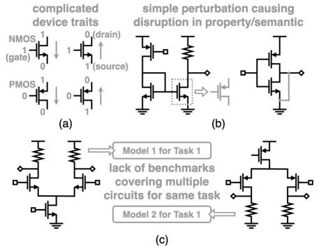
Figure 1: Three challenges in applying self-supervised graph representation learning on device-level circuits.

Second, traditional graph augmentation techniques, such as randomly adding nodes or edges, are inadequate for device-level circuits. As shown in Figure˜1(b), even a small change like adding an edge to the ground can fix the output voltage at zero and disrupt the circuit’s functionality. Logic synthesis tools [16, 17] can be useful in the data augmentation of gate-level digital circuits [18, 9], but these are not available for device-level circuits.

Third, there is a lack of benchmarks for device-level circuits that consider diverse circuit structures within each task. As illustrated in Figure˜1(c), previous works typically focus on topology-specific learning that applies separate models for different topologies [19, 20, 21, 22]. This highlights the need for a comprehensive cross-topology benchmark to better evaluate graph learning methods for device-level circuits.

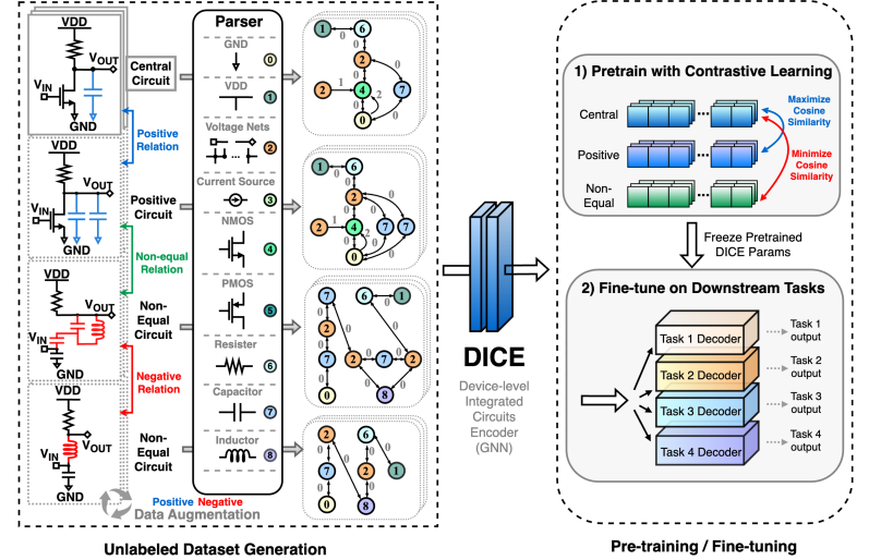
Figure 2: Overall framework. First, a large pretraining dataset is created by augmenting the initial circuits. Positive augmentation produces circuits with similar high-level semantics to the initial ones, while negative augmentation modifies these semantics. DICE is then pretrained using graph contrastive learning, maximizing similarity between central and positive circuits while minimizing it for unequal circuits. After pretraining, DICE is integrated into new models to solve various downstream tasks.

Considering these challenges, we propose DICE: Device-level Integrated Circuits Encoder, a pretrained graph neural network (GNN) applicable to both analog and digital circuits. As illustrated in Figure˜2, our method begins with a novel graph construction method that effectively distinguishes different net and device connections. Following this, we propose two customized data augmentation techniques described in Figure˜3. The augmentation either preserve or alter the high-level semantics of circuits, providing diversity to the pretraining dataset. Then, we design a contrastive learning loss considering three different relationships between circuits: positive, negative, and unequal. After pretraining, DICE is integrated to the full message passing neural network (MPNN) in Figure˜4 and evaluated on our proposed benchmark. The benchmark consists of three downstream tasks, each with multiple circuit topologies.

The contributions of our work are as follows:

• To the best of our knowledge, this is the first self-supervised graph representation learning method designed for device-level integrated circuits (IC).

• We propose a novel circuit-to-graph mapping that incorporates edge features to capture different interactions between voltage nets and transistors.

• We introduce two novel data augmentation techniques that do not use any circuit simulation or EDA tool.

• We present a benchmark comprising three graph learning tasks for device-level circuits, and all tasks are not restricted to a single circuit topology.

2 Preliminaries

Graph Contrastive Learning is one of the major self-supervised graph representation learning methods. These methods learn node, edge, or graph embeddings by maximizing similarities between positive (similar) samples and minimizing those between negative (dissimilar) samples. To enable the learning of robust representations applicable to various tasks, the approach frequently uses data augmentation for self-supervision [23], such as adding nodes or perturbing edges within the graph.

One of the most widely used objectives for contrastive learning is the NT-Xent loss [24]. Starting from $N$ number of data, each data is augmented twice to form $2N$ samples, forming $N$ positive pairs. For each sample $i\in\{1,2,\cdots,2N\}$, let $\mathbf{z}_{i}$ be its embedding and $\mathbf{z}_{j(i)}$ be the embedding of its positive counterpart. The NT-Xent loss is then given by:

$$\mathcal{L}_{\text{NT-Xent}}=\frac{1}{2N}\sum_{i=1}^{2N}-\log\frac{\exp\bigl{(}\mathrm{sim}(\mathbf{z}_{i},\mathbf{z}_{j(i)})/\tau\bigr{)}}{\sum_{k=1}^{2N}\mathbf{1}_{[k\neq i]}\exp\bigl{(}\mathrm{sim}(\mathbf{z}_{i},\mathbf{z}_{k})/\tau\bigr{)}}$$ (1)

where $\mathrm{sim}$ is a similarity function (i.e. cosine similarity) and $\tau$ is a temperature parameter. Minimizing $\mathcal{L}_{\text{NT-Xent}}$ clusters the features of positive pairs in the embedding space while pushing negative pairs apart, resulting in discriminative representations. In graph settings, contrastive learning can be operated in three levels: node, edge, and graph level. Depending on the targeting task, the inputs $\mathbf{z}$ in Eq. (1) can be either node, edge, or graph embeddings.

Graph Representation Learning on Digital Circuits. Logic gates, the basic components of digital circuits, can be constructed as directed acyclic graphs (DAGs) [25]. With these graphs, pioneering works have further pretrained models to reduce the excessive time and cost associated with large-scale digital hardware design. Both supervised [18, 8] and self-supervised [9, 10] pretraining methods exist for digital circuits, addressing tasks such as predicting functional similarities between circuit logics. To address data scarcity, these works utilize logic synthesis tools such as Yosys [16] and ABC [17], which generate augmented circuit views preserving identical functionalities. Recently, large language models (LLMs) have also been explored as one approach for augmenting digital circuit data [26, 27], which are also used for multimodal circuit representation learning [28]. However, despite numerous studies on digital circuit representation learning, these approaches cannot be applied to AMS circuits as they can not be represented just with logic gates.

Graph Representation Learning on AMS Circuits. Due to ambiguous signal directions, various graph construction methods have been proposed for AMS circuits. CktGNN [29] form a DAG by setting voltage nets as nodes, and basic operational amplifier circuits and passive devices as edges. Paragraph [11] represents both devices and voltage nets as nodes, while also distinguishing different edge types to predict layout parasitics using the attention mechanism. A supervised pretraining approach in [12] sets every device pins as separate nodes and pretrains GNN to predict DC voltage outputs. The learned representations are then applied to predict simulation results on unseen circuits. Other methods include considering AC and DC current paths as different edges [13], setting only nets as nodes [15], or setting only devices as nodes [14]. However, self-supervised pretraining methods remain underexplored, and one reason is the lack of a reliable data augmentation tool for AMS circuits. While previous works on data augmentation for AMS circuits [30, 31] exist, they are task-specific and primarily focus on analog circuits. Large language models (LLMs) can be an alternative as they can also generate AMS circuits at the device level [32], but their effectiveness as a data augmentation tool remains uncertain.

3 Method

Self-supervised pretraining for device-level circuits presents multiple challenges. A significant requirement is the development of an appropriate graph construction method that accurately addresses the signal ambiguity of device-level circuits (Figure˜1(a)). Additionally, there is a necessity for a tailored graph augmentation technique that preserves the high-level semantics inherent in circuit designs. To address these challenges, we propose DICE, the first self-supervised pretrained model for device-level circuits. In the following subsections, we will introduce a novel graph construction method for device-level circuits (Section˜3.1), a customized data augmentation method that leverages domain knowledge of devices in integrated circuits (Section˜3.2), and a contrastive learning framework based on our circuit augmentation scheme (Section˜3.3). Moreover, we also state our method on how we incorporated the pretrained model to solve diverse downstream tasks (Section˜3.4).

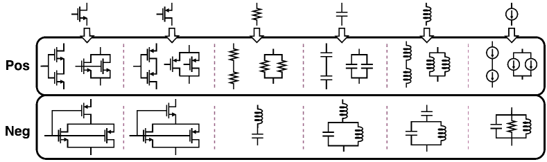
Figure 3: Positive and Negative Data Augmentation. Devices are modified while preserving all connections to other nodes. The theoretical intuition behind negative augmentation is detailed in Appendix A.

3.1 Graph Construction

The absence of a unified graph construction method for device-level circuits stems primarily from the complex interactions between transistor devices and the voltage nodes connected at each pin. Recent studies [12, 33] have modeled each device pin as a distinct node, separate from its corresponding device node. However, these methods utilize undirected edges, which fail to capture different types of connections between voltage nets and transistor devices. For instance, the voltage signal from a transistor’s gate influences the current flow through the transistor, but the transistor itself yields significantly less influence on the signal at the gate node. Similarly, the interactions between drain and source nodes and the transistor differ from those with the gate node. Previous approaches cannot distinguish these different connections.

To address this limitation, we introduce our new circuit-to-graph mapping designed specifically for device-level circuits. The left part of Figure˜2 illustrates our proposed circuit-to-graph conversion. To begin with, we utilize one-hot encoding to represent various device types and their connections, and form a homogeneous graph. There are nine distinct node types, which include: ground voltage net (0), power voltage net (1), other voltage nets (2), current source (3), NMOS (4), PMOS (5), resistor (6), capacitor (7), and inductor (8). The relationships among these devices are categorized into five edge types: current flow path (0), connections from voltage nets to NMOS gates (1) or bulks (2), and connections from voltage nets to PMOS gates (3) or bulks (4). Notably, the edges from gate and bulk voltage nets to MOSFETs are directed, as these nets exert significantly greater influence on the device than the device does on the nets. With these settings, our graph construction method makes full use of edge features without separating device pin nodes from their respective devices.

3.2 Positive and Negative Data Augmentation

Training a general-purpose model requires constructing a comprehensive dataset. A straightforward approach to creating a large-scale circuit dataset is to combine various device parameter configurations [34, 29]. However, this approach may not fully capture the breadth of circuit knowledge. Consider a circuit with twenty devices, each having three possible parameter values. This setup results in $3^{20}$ possible combinations, generating an enormous dataset from a single circuit. Yet, limiting each device to only three parameter values is unlikely to encompass the full complexity of circuit behavior, as useful parameters vary significantly across tasks and technologies. Furthermore, capturing structural information necessitates incorporating diverse circuit topologies, further expanding the dataset exponentially with inefficiency.

Therefore, instead of considering device parameters, we use data augmentation to generate a sufficiently large pretraining dataset that effectively captures structural differences between circuits. We introduce two data augmentation methods: positive and negative augmentation. Positive augmentation generates new circuit topologies while preserving the properties of the original circuit. In each iteration, a random device is selected, and an identical device is added either in parallel or in series as in Figure˜3. Although the device parameters are not considered, this modification is equivalent to changing the parameters of the selected device. This implies that the augmented graphs retain properties closely resembling those of the original graph. Samples generated with positive augmentation can be augmented again to generate new positive and negative samples. By maximizing the similarities between these positive samples, DICE captures the underlying semantics shared across different designs.

On the other hand, previous studies have found that the effectiveness of contrastive learning is closely related to the quality of negative samples [35, 36]. Therefore, we design another negative data augmentation technique to increase the diversity of samples. Specifically, this process involves randomly selecting a device and modifying it according to the rules in Figure˜3. The goal is to introduce significant changes in frequency response or DC voltage operation, and this modification results in a new topology that has distinct graph-level properties. Samples generated with negative augmentation cannot be augmented again, since the relationship between the initial circuit and the augmented view from that negative sample cannot be defined, meaning that automatic labeling with self-supervision is impossible for this case.

3.3 Graph Contrastive Pretraining

Once the dataset is prepared using data augmentation, graph-level contrastive learning is performed as illustrated in the upper right part of Figure˜2. Circuits that are either initial designs or their positively augmented variants are designated as central circuits, serving as the main targets of contrastive learning. Each central circuit has three types of relationships with other circuits in the batch: positive, negative, and unequal. A positive relationship indicates that a circuit shares similar high-level semantics with the central circuit, meaning it originates from the same initial design. A negative relationship arises when a circuit is generated through negative augmentation of the central circuit. Unequal relationships include circuits with different initial designs and their corresponding positive and negative augmentations.

After processing the batch of circuits through a GNN, graph-level features are extracted. Our contrastive learning framework then maximizes cosine similarities between central circuit features and their positive sample features while minimizing similarities with their unequal sample features.

Pretraining Model (DICE) Architecture. For graph-level feature extraction, we pretrain a graph isomorphism network (GIN) with depth 2, including the edge feature updates.

$$\begin{split}\mathbf{h}_{v}^{(1)}&=MLP_{\theta_{0}}(\mathbf{h}_{v}^{(0)}),\quad\mathbf{e}_{u\rightarrow v}^{(1)}=MLP_{\theta_{1}}(\mathbf{e}_{u\rightarrow v}^{(0)})\end{split}$$ (2)

$$\begin{split}\mathbf{m}_{v}^{(k)}&=\sum_{u\in\mathcal{N}(v)}\mathbf{h}_{v}^{(k)}\cdot\mathbf{e}_{u\rightarrow v}^{(k)},\\ \mathbf{h}_{v}^{(k+1)}&=MLP_{\theta_{2}^{(k)}}((1+\phi_{h}^{(k)})\cdot\mathbf{h}_{v}^{(k)}+\mathbf{m}_{v}^{(k)}),\\ \mathbf{e}_{u\rightarrow v}^{(k+1)}&=MLP_{\theta_{3}^{(k)}}((1+\phi_{e}^{(k)})\cdot\mathbf{e}_{u\rightarrow v}^{(k)}+\mathbf{m}_{u}^{(k)}-\mathbf{m}_{v}^{(k)})\\ \end{split}$$ (3)

$$\begin{split}\mathbf{g}_{(V,E)}&=\sum_{v\in V}\mathbf{h}_{v}^{(l+1)}+\sum_{u\rightarrow v\in E}\mathbf{e}_{u\rightarrow v}^{(l+1)}\end{split}$$ (4)

Eqs. (2)–(4) illustrates the node and edge feature update rules of DICE, where $\theta_{0},\theta_{1},\theta_{2}^{(k)},\theta_{3}^{(k)},\phi_{h}^{(k)},\phi_{e}^{(k)}$ are the training parameters. Batch normalization and dropout layers are included between linear layers. Eq. (2) matches the initial dimensions of node and edge features (9 and 5) to the hidden dimension value, and $\mathbf{h}_{u}^{(0)}$, $\mathbf{e}_{v\rightarrow u}^{(0)}$ are the initial one-hot encoding of node and edge types. Eq. (3) explains the message passing rule, where $k=1,...,l$ and $l(=2)$ is the depth of the GNN. The graph-level feature $\mathbf{g}_{(V,E)}$ is calculated in Eq. (4), by summing all the updated node and edge features within each graph $G=(V,E)$.

Loss Function. In each batch, a joint distribution of $(x,x^{+})$ exists, representing the distribution of two circuits with a positive relationship. Given an arbitrary central circuit $x_{i}$ in this distribution, let $X_{i}^{+}$ and $X_{i}^{-}$ denote the sets of positive and negative augmented views derived from the same initial design as $x_{i}$, respectively. Also, let $X_{i}^{\neq}$ be the set of circuits unequal to $x_{i}$. The union $X_{i}^{+}\cup X_{i}^{-}\cup X_{i}^{\neq}$ forms the complete set of circuits in the batch, ensuring no overlap between the sets. The objective is to maximize cosine similarities between $x_{i}$ and $x_{i}^{+}\in X_{i}^{+}$, while minimizing similarities between $x_{i}$ and $x_{i}^{\neq}\in X_{i}^{\neq}$. Minimization between $x_{i}$ and $x_{i}^{-}$ is excluded since they share similar topological structures, originating from the same initial circuit. However, their high-level semantics differ, so their similarities are also not maximized. Although the similarities between $x_{i}$ and circuits in $X_{i}^{-}$ are neither maximized nor minimized, when considering other central circuit $x_{j\neq i}$ with different initial design, circuits in $X_{i}^{-}$ are included in $X_{j}^{\neq}$. As a result, the similarities between these circuits and $x_{j}$ are minimized.

$$L_{\theta}=\mathbb{E}\bigg{[}{-\log\frac{e^{{f_{\theta}(x,x^{+})}/{\tau}}}{\underset{z\in X^{+}}{\sum}e^{{f_{\theta}(x,z)}/{\tau_{p}}}+\underset{z\in X^{\neq}}{\sum}e^{{f_{\theta}(x,z)}/{\tau_{n}}}}\bigg{]}}$$ (5)

Building on this, we introduce a loss variant of Eq.(1), formulated in Eq.(5). The GNN feature extractor $f_{\theta}$, parameterized by $\theta$, computes the cosine similarity between the graph features of two input graphs using temperature coefficients $\tau$, $\tau_{p}$ and $\tau_{n}$. The expectation is computed over the joint probability distribution of $(x,x^{+})$, and $X^{+},X^{\neq}$ denote the sets of positive and unequal circuits, respectively, for an arbitrary circuit $x$ in the distribution. Details on the algorithm and loss calculation are provided in Appendix B.

3.4 Application to Downstream Tasks

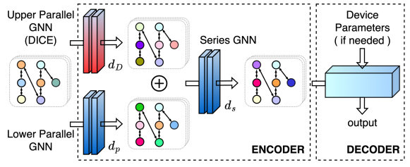
Figure 4: Model Architecture for Downstream Tasks.

After pretraining, we integrate DICE into the full message passing neural network (MPNN) model shown in Figure˜4 to address diverse downstream tasks. The encoder consists of three GNNs: two parallel networks that process the same graph input, followed by a series-connected network. One of the parallel GNNs is either initialized and frozen with pretrained DICE parameters, while the other parallel GNN and the series-connected GNN remain fully trainable. The encoder remains fixed for each downstream task if all GNN depth values are specified. We define $d_{D},d_{p},d_{s}$ as the depths of the GNNs in DICE, the parallel GNN other than DICE, and the series-connected GNN, respectively.

The decoder network takes the output graph from the encoder as input and incorporates device parameters if required by the downstream task. To encode device parameters, we represent each device type using a 9-dimensional one-hot vector, scaled by its respective parameter values. Since parameter values vary significantly in magnitude across devices, we apply a negative logarithmic transformation before scaling. These encoded parameters are then concatenated with the node features from the encoder output and passed through the subsequent layers of the decoder.

4 Experiments

We first outline the experimental setup and present pretraining results. Next, we evaluate the model on three downstream tasks, each involving graph-level prediction. Hyperparameters for all training are detailed in Appendix C.1.

4.1 Pretraining

Settings. The dataset comprises 55 initial circuit topologies, including both analog and digital designs. For pretraining, 40 topologies are each augmented $\times 4000$ ($\times 2000$ positive and $\times 2000$ negative), yielding a training dataset of 160,000 graphs. Similarly, all 55 topologies are augmented $\times 500$ for both validation and test sets, resulting in 27,500 graphs each. Data augmentation is performed independently for generating the training, validation, and test datasets.

Results. Figure˜5 presents the t-SNE plots of the graph embedding vectors. Each of the 55 different colors represents a unique initial circuit, and its augmented views are marked the same color as the corresponding initial circuit. Figure˜5(c) shows significant improvements in clustering compared to Figure˜5(a) and (b), providing evidence of successful pretraining. To further validate these results, we computed the mean and standard deviation of cosine similarities. Table 1 presents the cosine similarities between samples within $X_{+}$ (positive pairs), between $X_{+}$ and $X_{\neq}$ (unequal pairs), and between $X_{+}$ and $X_{-}$ (negative pairs). The results confirm that similarities are minimized between unequally related samples while remaining high between positively related pairs. A key observation is that cosine similarity is also minimized between negatively related samples, even without explicit minimization in the loss function.

Figure 5: t-SNE visualization of graph-level features for 55 circuit topologies in the test dataset. Each plot represents: (a) initial embeddings, (b) embeddings processed by an untrained GNN, and (c) embeddings processed by DICE.

Table 1: Cosine Similarities of Graphs in the Test Dataset. Means/standard deviations are computed with five seeds.

Graph Embeddings	Positive Pairs	Unequal Pairs	Negative Pairs
Initial	$0.9983\pm 0.0026$	$0.9825\pm 0.0200$	$0.9825\pm 0.0200$
untrained GNN	$0.9977\pm 0.0037$	$0.9804\pm 0.0205$	$0.9825\pm 0.0200$
DICE	$0.9406\pm 0.1412$	$\textbf{0.2349}\pm 0.4594$	$\textbf{0.1393}\pm 0.2864$

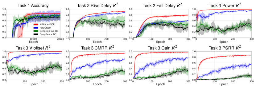
Figure 6: Performance of Baselines during Downstream Task Training. MPNN w DICE is our model and ParaGraph represents the GNN model used in [11]. DeepGen w/o DC and DeepGen w DC indicates the GNN backbone used in [12]. We did not pretrain DeepGen w/o DC, and pretrained DeepGen w DC to predict the node voltage values on 6 different circuit topologies. In each plot, $\mu\pm\sigma$ range is shown for all models trained with 3 different seeds.

Table 2: Comparison with the baseline models. We train each model three times using different seeds and report the average performance.

Baselines	Task 1 (%)	Task 2 ($R^{2}$)		Task 3 ($R^{2}$)
	Accuracy	Rise Delay	Fall Delay	Power	V${}_{\text{offset}}$	CMRR	Gain	PSRR
[11]	91.42	0.9255	0.6373	0.9312	0.9585	0.7912	0.8488	0.6215
[12]${}_{\text{unpretrained}}$	85.02	0.8866	0.6715	0.8403	0.8478	0.5637	0.6813	0.3820
[12]${}_{\text{pretrained}}$	84.65	0.9131	0.6875	0.4479	0.5190	0.3246	0.3454	0.0851
DICE(2,0,2)	93.94	0.9468	0.8085	0.9916	0.9950	0.9374	0.9769	0.8809

4.2 Finetuning on Downstream Tasks

We evaluate the generalizability of DICE across three graph-level prediction tasks. Detailed settings for each task are provided in Appendix C.1.

Task 1: Circuit Similarity Prediction. This task involves predicting the relative similarities between circuits, including both analog and digital topologies. The objective is to maximize prediction accuracy based on true similarity, which is determined by the number of shared labels: analog, digital, delay lines, amplifiers, logic gates, and oscillators.

Task 2: Delay Prediction. In Task 2, the model is trained to predict simulation results for five digital delay line circuits. Each simulation records two values: the time difference between the rising edges and the falling edges of the input and output clock signals. The objective is to maximize $R^{2}$ across all simulations.

Task 3: OPAMP Metric Prediction. This task focuses on predicting simulation results for five analog operational amplifier (OPAMP) circuits. Each simulation records five values: power, DC voltage offset (V${}_{\text{offset}}$), common mode rejection ratio (CMRR), gain, and power supply rejection ratio (PSRR). The goal is to maximize $R^{2}$ across all simulations.

Comparison with baselines. We included three baseline models to demonstrate the superiority of DICE in device-level circuit representation learning. For a fair comparison, we selected previous works that (1) explicitly define graph construction using transistors, (2) employ GNNs, and (3) predict circuit simulation results [11, 12]. Similar to our approach, [11] represents both devices and voltage nets as graph nodes while distinguishing different connections using multiple edge types. However, unlike our homogeneous graph construction, they utilize a heterogeneous GNN with an attention mechanism and do not include power and ground voltage nets as nodes. [12] pretrains the GNN proposed in [37] using a node-level DC voltage prediction task, which is a supervised method. Additionally, their graph construction does not distinguish between edge types and separates device pins into individual nodes apart from their corresponding devices. From this work, we selected both pretrained and unpretrained GNNs as baseline models. The GNN models from the selected works serve as the encoder for solving the three downstream tasks in our benchmark, while the decoders remain identical across all models including our MPNN model. We compare these baselines with our model using the architecture in Figure˜4, which has a GNN depth configuration of $(d_{D},d_{p},d_{s})=(2,0,2)$.

Ablation study. We also conducted an ablation study to further demonstrate the effectiveness of DICE. We built and compared two different models: one incorporating, and the other not incorporating DICE. These models are designed to have the same number of training parameters, following the architecture in Figure˜4. We evaluated results for six possible combinations of GNN depths $(d_{p},d_{s})=(0,0),(0,1),(1,0),(1,1),(0,2),(2,0)$. $d_{D}$ is set to 0 when the model excludes DICE and to 2 when the model includes DICE. While the encoder is fixed across all downstream tasks, the decoder varies but remains consistent across equivalent tasks.

Table 3: Comparison on models with and without DICE. DICE leads to significant performance gain.

($d_{D},d_{p},d_{s}$)		Task 1 (%)	Task 2 ($R^{2}$)		Task 3 ($R^{2}$)
		Accuracy	Rise Delay	Fall Delay	Power	Voffset	CMRR	Gain	PSRR
MPNN without DICE	(0, 0, 0)	76.91	0.7541	0.5456	0.9651	0.8261	0.4794	0.3754	0.2798
	(0, 0, 1)	74.84	0.7706	0.5486	0.9718	0.8976	0.6384	0.6441	0.5024
	(0, 1, 0)	77.90	0.7666	0.5405	0.9636	0.8825	0.6019	0.6013	0.4501
	(0, 1, 1)	84.68	0.9404	0.8124	0.9827	0.9876	0.9125	0.9633	0.8064
	(0, 0, 2)	88.57	0.9229	0.7790	0.9745	0.9863	0.9091	0.9605	0.7929
	(0, 2, 0)	86.28	0.9237	0.7618	0.9866	0.9867	0.9066	0.9610	0.7900
MPNN with DICE	(2, 0, 0)	92.13	0.9352	0.7885	0.9769	0.9820	0.8865	0.9402	0.7535
	(2, 0, 1)	93.41	0.9310	0.7805	0.9904	0.9876	0.9167	0.9659	0.8132
	(2, 1, 0)	93.43	0.9294	0.7820	0.9849	0.9868	0.9147	0.9634	0.8061
	(2, 1, 1)	94.54	0.9417	0.7873	0.9847	0.9872	0.9147	0.9627	0.8061
	(2, 0, 2)	94.01	0.9231	0.8134	0.9918	0.9950	0.9371	0.9769	0.8776
	(2, 2, 0)	93.98	0.9402	0.7851	0.9876	0.9874	0.9165	0.9641	0.8055

Results. We first show the comparison between the baseline models and DICE on all three downstream tasks. In  Figure˜6, we show the performance curves of all models on the validation dataset during training. Furthermore, the detailed final performance comparison on each task is listed in Table. 2. To eliminate uncertainty, we trained each model with three different seeds and report the average performance values from all three models. Results show that our model outperforms baselines in all downstream tasks.

The results of the ablation study are presented in Table 3, which compares the performance of two MPNN models: one with and the other without DICE. The number of training parameters is kept equal when the depths of the parallel and series GNNs $(d_{p},d_{s})$ are the same, serving as comparable configurations. A total of 36 models are trained and values in Table 3 are highlighted if the final performance surpasses that of the corresponding configuration. Except for some cases in $(d_{p},d_{s})=(1,1)$, all highlighted values correspond to the MPNN model with DICE. This confirms the effectiveness of our pretraining method in capturing the underlying knowledge of device-level circuits. Additionally, the best final performance values, marked with underlines, are all achieved by the MPNN model with DICE.

Discussions. We make three key observations. First, training models with DICE is highly stable. Unlike other baseline models in Figure˜6, performance plots remain consistent across different seeds, demonstrating robust training stability. Second, in some cases, DICE outperforms GNNs trained from scratch. For example, in Table. 3, models with $(d_{D},d_{p},d_{s})=(2,0,0),(0,2,0),(0,0,2)$ have the same total number of parameters. However, $(2,0,0)$ does not include additional trainable GNN layers. Despite this, it achieves better results on Task 2, suggesting that DICE contributes significantly to model performance. Third, even unpretrained GNN models outperform baselines. For instance, models with $(d_{D},d_{p},d_{s})=(0,1,1),(0,2,0),(0,0,2)$ in Table 3 generally achieve higher performance than the baselines in Table 2. This provides evidence that our graph construction method is effective compared to previous approaches.

5 Conclusion

In this work, we propose DICE, a pretrained GNN model designed for general tasks in device-level integrated circuits. Our two novel data augmentation techniques mitigate the scarcity of circuit data, while graph-level contrastive learning enables task-agnostic pretraining. The major contribution of this work is the introduction of the first self-supervised graph representation learning framework for device-level circuits. We argue that device-level interpretation provides a more general and flexible way to represent integrated circuits compared to logic gate-level representations, as it accommodates both analog and digital circuits. Additional contributions include a novel circuit-to-graph mapping technique and the introduction of a device-level circuit benchmark, where all three tasks require handling multiple circuit topologies simultaneously. Experimental results demonstrate that applying DICE leads to significant improvements across all three downstream tasks. Furthermore, compared to previous graph learning methods for device-level circuits, our approach outperforms all prior models across all performance metrics on the proposed benchmark. We envision this work as a stepping stone toward developing powerful foundational models for device-level circuits.

6 Limitations and Future Work

Graph representation learning for AMS circuits is still in its early stages. In this work, we focused on the main contributions while omitting detailed comparisons of minor aspects of our framework. Nevertheless, we believe our work opens several promising research directions.

First, more comprehensive comparisons are required for graph construction methods. While our method empirically outperforms others across three downstream tasks, more sophisticated evaluations—such as graph isomorphism tests—could provide deeper insights into the optimal graph.

Second, exploring alternative machine learning techniques could further enhance performance. For example, graph transformers may better leverage global structural information. Other graph representation learning methods, such as graph autoencoders and node/edge masking techniques, also hold potential for future exploration.

Third, solving more complex EDA tasks would provide stronger validation of the pretrained model’s effectiveness. Solving large-scale circuit timing prediction, congestion prediction, and sizing devices for optimal circuit performance represent a valuable avenue for further research.

Appendix A Details of Negative Data Augmentation

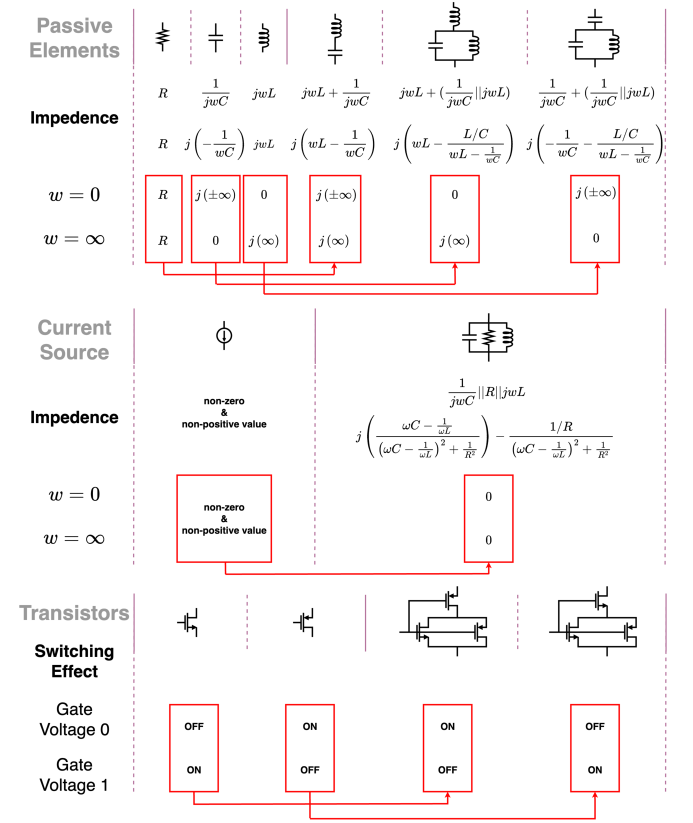
Figure 7: Conversion of characteristics through negative data augmentation.

In this section, we detail the augmentation of negative data corresponding to positive instances. For passive elements, we consider their impedance at DC (zero frequency) and in the high-frequency limit, modifying them to exhibit inverse impedance characteristics at both extremes. For current sources, which supply energy, we replace them with passive elements, as the latter primarily dissipate energy. Finally, for transistors, we account for switching behavior based on gate voltage and introduce counterpart transistors in both parallel and series configurations to invert this behavior, ensuring the corresponding negative design exhibits the opposite functionality.

Appendix B Details of Contrastive Learning

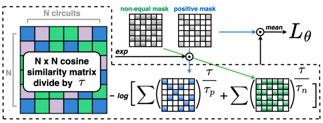
Figure 8: Masking operation. $\odot$ indicates the hadamard product (element-wise multiplication) between matrices.

Masking is our key source of rapid pretraining, with the cost of GPU memory. Algorithm. 1 provides the pseudocode and Fig. 8 visualize the details of the the proposed masking for contrastive learning. For each batch, we first matched the number of graphs for every circuit types. For example, consider the case when the number of graphs originated from the inverter circuit is 5. If this is the minimum number among all other circuit types in the batch, then 5 circuits are sampled for every circuit types and form a new batch. Then, the cosine similarity matrix is formed with graph-level features in the batch with masks indicating positive and non-equal. Element-wise products between the similarity matrix and the masks filter out the unnecessary parts in parallel. Multiple positive pairs are considered simultaneously with this operation, thereby significantly reducing the training speed with the cost of GPU memory.

Algorithm 1 Graph-level Contrastive Learning

Input: dataset with augmentation ($\textstyle\chi$), epoch ($T$), temperature coefficients ($\tau_{p}$, $\tau$, $\tau_{n}$), learning rate ($\eta$)

Output: pretrained model parameter ($\theta_{T}$)

Initialize: model parameter $\theta_{0}$

1: for $t=0,1,2,...,T-1$ do
2: for batch $B$ in $\textstyle\chi$ do

3:  $m$ $\leftarrow$ min number covering all circuit types in $B$

4:  $B_{m}$ $\leftarrow$ batch$\in\mathbb{R}^{L}$ having $m$ graphs for all circuit types (maintaining circuit diversity for every batch)

5:  $g$ $\leftarrow$ $GNN_{\theta_{t}}(B_{m})$: graph-level features $\in\mathbb{R}^{L\times h}$

6:  $S$ $\leftarrow$ $gg^{T}$: cosine similarity matrix $\in\mathbb{R}^{L\times L}$

7:  $M_{+},M_{\neq}$ $\leftarrow$ Mask matrices $\in\mathbb{R}^{L\times L}$ for positive and non-equal pairs

9:  $L_{\theta_{t}}$ $\leftarrow\sum(M_{+}\ast\big{[}S/\tau-\log(\sum M_{+}\ast e^{S/\tau_{p}}+\sum M_{\neq}\ast e^{S/\tau_{n}})\big{]})/\sum M_{+}$

10:  ​​​$\theta_{t+1}$ $\leftarrow\theta_{t}-\eta\nabla_{\theta_{t}}L_{\theta_{t}}$

11: end for

12: end for

Appendix C Details of the Experiments

C.1 Hyperparameters

Training parameters	DICE Pretraining	[12] Pretraining	Downstream Task 1	Downstream Task 2	Downstream Task 3
learning rate	0.0003	0.000005	0.00001	0.0001	0.0001
batch size	1024	1024	50	2048	1024
epochs	200	200	20000	300	300
$(\tau_{p},\tau,\tau_{n})$	(0.2, 0.05, 0.05)	–	–	–	–

Hyperparameters	DICE	Encoder	Decoder	DeepGEN in [12]
hidden dimension	256	512	256	512
dropout probability	0.2	–	0.3	–
activation	GELU	GELU	GELU	GELU
GNN type	GIN	GIN	–	GAT
GNN depth	2	depends	0	3

C.2 Settings of Downstream Tasks

Task 1: Circuit Similarity Prediction (Analog + Digital). The training dataset consists of 50 circuits, including the 40 topologies from the pretraining dataset. The validation and test datasets each contain 5 additional circuits, resulting in a total of 55 circuits. Given a target circuit and two comparison circuits, the model outputs a three-dimensional probability distribution: whether the first circuit is more similar, the second circuit is more similar, or the two circuits are equally similar to the target circuit. In each training step, one target circuit from the training dataset is sampled, and all permuted pairs across the 50 circuits form a tensor of size $(50\times 49=2950,\ \ 3\times graph\ feature\ dimension)$ for the training model. Based on the number of shared labels, the logits indicating similarity comparisons are computed. Using these logits and the model’s output, the cross-entropy loss is calculated and minimized.

Task 2: Predicting Rise and Fall Delays on Five Delay Line Circuits (Digital). For simulation, we used NGSPICE with BSIM4 45nm technology, which are the open-source circuit simulator and the technology file. The delay line circuits for task 2 are not included in the pretraining dataset, and the simulation result dataset includes 45,000 device parameter combinations for each topology. The dataset is split into 8:1:1 ratio for train, validation, and test dataset. The output dimension of the decoder model is 2.

Task 3. Predicting Five different Metrics on Five Operational Amplifier Circuits (Analog). NGSPICE with BSIM4 45nm technology file is also used for task 3. The OPAMP circuits for task 3 are included in the pretraining dataset, and the simulation result dataset consists of 60,000 device parameter combinations for each topology. Circuits and testbench files are sourced from the work in [38], and the train, validation, and test datasets are split into 8:1:1 ratio. The decoder network used in Task 3 is identical to that in Task 2, except that the output dimension is set to 5.

References

- [1] William L Hamilton, Rex Ying, and Jure Leskovec. Representation learning on graphs: Methods and applications. arXiv preprint arXiv:1709.05584, 2017.
- [2] William L Hamilton. Graph representation learning. Morgan & Claypool Publishers, 2020.
- [3] Wei Jin, Tyler Derr, Haochen Liu, Yiqi Wang, Suhang Wang, Zitao Liu, and Jiliang Tang. Self-supervised learning on graphs: Deep insights and new direction. arXiv preprint arXiv:2006.10141, 2020.
- [4] Lirong Wu, Haitao Lin, Cheng Tan, Zhangyang Gao, and Stan Z Li. Self-supervised learning on graphs: Contrastive, generative, or predictive. IEEE Transactions on Knowledge and Data Engineering, 35(4):4216–4235, 2021.
- [5] Marzyeh Ghassemi, Tristan Naumann, Peter Schulam, Andrew L Beam, Irene Y Chen, and Rajesh Ranganath. A review of challenges and opportunities in machine learning for health. AMIA Summits on Translational Science Proceedings, 2020:191, 2020.
- [6] Xuan Zang, Xianbing Zhao, and Buzhou Tang. Hierarchical molecular graph self-supervised learning for property prediction. Communications Chemistry, 6(1):34, 2023.
- [7] Lei Chen, Yiqi Chen, Zhufei Chu, Wenji Fang, Tsung-Yi Ho, Ru Huang, Yu Huang, Sadaf Khan, Min Li, Xingquan Li, et al. The dawn of ai-native eda: Opportunities and challenges of large circuit models. arXiv preprint arXiv:2403.07257, 2024.
- [8] Zhengyuan Shi, Hongyang Pan, Sadaf Khan, Min Li, Yi Liu, Junhua Huang, Hui-Ling Zhen, Mingxuan Yuan, Zhufei Chu, and Qiang Xu. DeepGate2: Functionality-aware circuit representation learning. In IEEE/ACM International Conference on Computer Aided Design (ICCAD), pages 1–9, 2023.
- [9] Ziyi Wang, Chen Bai, Zhuolun He, Guangliang Zhang, Qiang Xu, Tsung-Yi Ho, Bei Yu, and Yu Huang. Functionality matters in netlist representation learning. In Proceedings of the 59th ACM/IEEE Design Automation Conference, pages 61–66, 2022.
- [10] Ziyi Wang, Chen Bai, Zhuolun He, Guangliang Zhang, Qiang Xu, Tsung-Yi Ho, Yu Huang, and Bei Yu. Fgnn2: A powerful pre-training framework for learning the logic functionality of circuits. IEEE Transactions on Computer-Aided Design of Integrated Circuits and Systems, 2024.
- [11] Haoxing Ren, George F Kokai, Walker J Turner, and Ting-Sheng Ku. Paragraph: Layout parasitics and device parameter prediction using graph neural networks. In 2020 57th ACM/IEEE Design Automation Conference (DAC), pages 1–6. IEEE, 2020.
- [12] Kourosh Hakhamaneshi, Marcel Nassar, Mariano Phielipp, Pieter Abbeel, and Vladimir Stojanovic. Pretraining graph neural networks for few-shot analog circuit modeling and design. IEEE Transactions on Computer-Aided Design of Integrated Circuits and Systems, 42(7):2163–2173, 2022.
- [13] Zonghao Li and Anthony Chan Carusone. Design and optimization of low-dropout voltage regulator using relational graph neural network and reinforcement learning in open-source sky130 process. In 2023 IEEE/ACM International Conference on Computer Aided Design (ICCAD), pages 01–09. IEEE, 2023.
- [14] Yusuke Yamakaji, Hayaru Shouno, and Kunihiko Fukushima. Circuit2graph: Circuits with graph neural networks. IEEE Access, 2024.
- [15] Jiqing Jiang, Yongqiang Duan, and Zhou Jin. Boosting the performance of transistor-level circuit simulation with gnn. 2025.
- [16] Clifford Wolf, Johann Glaser, and Johannes Kepler. Yosys-a free verilog synthesis suite. In Proceedings of the 21st Austrian Workshop on Microelectronics (Austrochip), volume 97, 2013.
- [17] Robert Brayton and Alan Mishchenko. Abc: An academic industrial-strength verification tool. In Computer Aided Verification: 22nd International Conference, CAV 2010, Edinburgh, UK, July 15-19, 2010. Proceedings 22, pages 24–40. Springer, 2010.
- [18] Min Li, Sadaf Khan, Zhengyuan Shi, Naixing Wang, Huang Yu, and Qiang Xu. Deepgate: Learning neural representations of logic gates. In Proceedings of the 59th ACM/IEEE Design Automation Conference, pages 667–672, 2022.
- [19] Keertana Settaluri, Ameer Haj-Ali, Qijing Huang, Kourosh Hakhamaneshi, and Borivoje Nikolic. Autockt: Deep reinforcement learning of analog circuit designs. In 2020 Design, Automation & Test in Europe Conference & Exhibition (DATE), pages 490–495. IEEE, 2020.
- [20] Ahmet F Budak, Prateek Bhansali, Bo Liu, Nan Sun, David Z Pan, and Chandramouli V Kashyap. Dnn-opt: An rl inspired optimization for analog circuit sizing using deep neural networks. In 2021 58th ACM/IEEE Design Automation Conference (DAC), pages 1219–1224. IEEE, 2021.
- [21] Souradip Poddar, Youngmin Oh, Yao Lai, Hanqing Zhu, Bosun Hwang, and David Z Pan. Insight: Universal neural simulator for analog circuits harnessing autoregressive transformers. arXiv preprint arXiv:2407.07346, 2024.
- [22] Zihu Wang, Karthik NS Somayaji, and Peng Li. Learn-by-compare: Analog performance prediction using contrastive regression with design knowledge. In Proceedings of the 61st ACM/IEEE Design Automation Conference, pages 1–6, 2024.
- [23] Tong Zhao, Yozen Liu, Leonardo Neves, Oliver Woodford, Meng Jiang, and Neil Shah. Data augmentation for graph neural networks. In Proceedings of the aaai conference on artificial intelligence, volume 35, pages 11015–11023, 2021.
- [24] Ting Chen, Simon Kornblith, Mohammad Norouzi, and Geoffrey Hinton. A simple framework for contrastive learning of visual representations. In International conference on machine learning, pages 1597–1607. PMLR, 2020.
- [25] Alan Mishchenko, Satrajit Chatterjee, and Robert Brayton. Dag-aware aig rewriting a fresh look at combinational logic synthesis. In Proceedings of the 43rd annual Design Automation Conference, pages 532–535, 2006.
- [26] Kaiyan Chang, Kun Wang, Nan Yang, Ying Wang, Dantong Jin, Wenlong Zhu, Zhirong Chen, Cangyuan Li, Hao Yan, Yunhao Zhou, et al. Data is all you need: Finetuning llms for chip design via an automated design-data augmentation framework. In Proceedings of the 61st ACM/IEEE Design Automation Conference, pages 1–6, 2024.
- [27] Mingjie Liu, Nathaniel Pinckney, Brucek Khailany, and Haoxing Ren. Verilogeval: Evaluating large language models for verilog code generation. In 2023 IEEE/ACM International Conference on Computer Aided Design (ICCAD), pages 1–8. IEEE, 2023.
- [28] Anonymous. Circuitfusion: Multimodal circuit representation learning for agile chip design. In The Thirteenth International Conference on Learning Representations, 2025.
- [29] Zehao Dong, Weidong Cao, Muhan Zhang, Dacheng Tao, Yixin Chen, and Xuan Zhang. Cktgnn: Circuit graph neural network for electronic design automation. arXiv preprint arXiv:2308.16406, 2023.
- [30] Ali Deeb, Abdalrahman Ibrahim, Mohamed Salem, Joachim Pichler, Sergii Tkachov, Anjeza Karaj, Fadi Al Machot, and Kyamakya Kyandoghere. A robust automated analog circuits classification involving a graph neural network and a novel data augmentation strategy. Sensors, 23(6):2989, 2023.
- [31] Ali Deeb, Mohamed Salem, Abdalrahman Ibrahim, Joachim Pichler, Sergii Tkachov, Karaj Anjeza, Fadi Al Machot, and Kyandoghere Kyamakya. A graph attention network based system for robust analog circuits’ structure recognition involving a novel data augmentation technique. IEEE Access, 12:29308–29344, 2024.
- [32] Yao Lai, Sungyoung Lee, Guojin Chen, Souradip Poddar, Mengkang Hu, David Z Pan, and Ping Luo. Analogcoder: Analog circuit design via training-free code generation. arXiv preprint arXiv:2405.14918, 2024.
- [33] Anonymous. Analoggenie: A generative engine for automatic discovery of analog circuit topologies. In The Thirteenth International Conference on Learning Representations, 2025.
- [34] Asal Mehradfar, Xuzhe Zhao, Yue Niu, Sara Babakniya, Mahdi Alesheikh, Hamidreza Aghasi, and Salman Avestimehr. Aicircuit: A multi-level dataset and benchmark for ai-driven analog integrated circuit design. arXiv preprint arXiv:2407.18272, 2024.
- [35] Rui Cao, Yihao Wang, Yuxin Liang, Ling Gao, Jie Zheng, Jie Ren, and Zheng Wang. Exploring the impact of negative samples of contrastive learning: A case study of sentence embedding. arXiv preprint arXiv:2202.13093, 2022.
- [36] Juncheng Zhou, Lijuan Zhang, Yachen He, Rongli Fan, Lei Zhang, and Jian Wan. A novel negative sample generation method for contrastive learning in hierarchical text classification. In Proceedings of the 31st International Conference on Computational Linguistics, pages 5645–5655, 2025.
- [37] Guohao Li, Chenxin Xiong, Ali Thabet, and Bernard Ghanem. Deepergcn: All you need to train deeper gcns. arXiv preprint arXiv:2006.07739, 2020.
- [38] Jintao Li, Haochang Zhi, Ruiyu Lyu, Wangzhen Li, Zhaori Bi, Keren Zhu, Yanhan Zeng, Weiwei Shan, Changhao Yan, Fan Yang, et al. Analoggym: An open and practical testing suite for analog circuit synthesis. arXiv preprint arXiv:2409.08534, 2024.