Kitaev-Ising-$J_{1}$-$J_{2}$ model: a density matrix renormalization group study

Abstract

We numerically study the Kitaev honeycomb model with the additional XX Ising interaction between the nearest and the next nearest neighbors (Kitaev-Ising-$J_{1}$-$J_{2}$ model), by using the density matrix renormalization group (DMRG) method. Such additional interaction correspond to the nearest and diagonal interactions on the square lattice. Phase diagram of the bare Kitaev model consist of low entangled commensurate magnetic phases and entagled Kitaev spin liquid. Anisotropic Ising interaction allows the entangled incommensurate magnetic phases in the phase diagram, which previously was predicted only for more complex type of interactions. We study the scaling law of the entanglement entropy and the bond dimension of the matrix product state with the size of the system. In addition, we propose an optimization algorithm to prevent DMRG from getting stuck in the low-entangled phases.

I Introduction

A quantum spin liquid (QSL) is a novel phase in condensed matter physics, characterized by the absence of long-range magnetic order due to strong quantum fluctuations, so electron spins do not form an ordered pattern but remain liquid-like even at zero temperature [1, 2, 3, 4, 5]. QSLs have been extensively studied due to their rich physics and unusual properties, including intriguing topological characteristics [6, 7] and supporting fractional excitations [8, 9]. QSLs play an important role in understanding strongly correlated materials [10, 11, 12] and have the potential to serve as platforms for topological quantum computation in the future [13].

The Kitaev honeycomb model [13] is an exactly solvable model whose ground state hosts both gapped and gapless $\mathbb{Z}_{2}$ quantum spin liquids (QSLs). The exact solution demonstrates that, in the Kitaev spin liquid (KSL), spins fractionalize into emergent quasiparticles—Majorana fermions. One of the key advantages of the Kitaev model is its conceptual simplicity, which makes it a promising candidate for experimental realization. However, identifying material realizations of KSLs remains challenging due to the absence of a conventional order parameter [14, 4]. Recently, various iridate and ruthenate compounds have been proposed as potential platforms for realizing KSLs [15, 16, 17, 18, 19, 20, 21].

To explain Kitaev physics in real materials, numerous extended Kitaev models have been proposed and extensively studied. Historically, the first extension of the Kitaev model was the inclusion of the isotropic nearest-neighbor (NN) Heisenberg interaction $J$, which arises from the direct overlap of $d$-orbitals (Kitaev-Heisenberg model) [15, 22, 23, 24, 25]. Later, it was shown in [26] that an additional bond-dependent anisotropic spin-exchange interaction exists between NN sites, commonly referred to as the $\Gamma$ coupling (Kitaev-Heisenberg-Gamma model). The $\Gamma$ interaction is highly frustrated and is the second strongest interaction in Kitaev materials, leading to a complex interplay with Kitaev interactions [26, 27, 28, 29, 30, 31, 32, 33]. A more realistic model must also account for the effects of trigonal splitting of the $t_{2g}$ orbitals, which induces an additional anisotropic coupling $\Gamma^{\prime}$, which is not symmetry-allowed in the absence of the trigonal distortion [26]. Other perturbations present in real materials have also been investigated, including the second-neighbor Kitaev interaction $K_{2}$ [34], and the second- and third-neighbor Heisenberg interactions $J_{2}$, $J_{3}$ [35, 36].

Another approach to realizing exotic phases of condensed matter is through quantum simulations, where quantum-mechanical devices are used to mimic and investigate quantum matter [37, 38]. Quantum spin liquids (QSLs) can be realized using Rydberg atom quantum simulators [39] (toric code-type QSL) or quantum processors [40] (Kitaev toric code). Despite significant progress in quantum computing and simulation, relatively high error rates in two-qubit gates remain a challenge [41]. One of the major source of the gate error comes from the non-ideal interactions that induce parasitic coupling between NN and next-nearest-neighbor (NNN) qubits. These interactions are described by an XX (or YY) Ising-like interaction between NN and NNN qubits [42, 43].

The DMRG is a powerful numerical method for computing properties of one-dimensional (1D) quantum systems and is widely regarded as the most effective technique for 1D systems [44, 45]. The DMRG algorithm optimizes a matrix product state (MPS)[46, 47, 48], a robust ansatz represented as a 1D tensor network. The computational cost of DMRG for a system with $N$ sites scales as $O(ND^{3})$, where $D$ is the bond dimension, which determines the size of the MPS and its capacity to capture quantum entanglement. The key reason for the success of DMRG is that the ground states of local Hamiltonians obey the area law [49, 50, 51, 52]. This implies that the ground states of local Hamiltonians can be accurately represented by MPS with a fixed bond dimension $D$, which grows exponentially with the entanglement entropy $S$, where $S$ scales with the system size $N$. Consequently, the computational cost is constrained by the area law of entanglement entropy. Thus, DMRG is highly efficient for 1D systems, where $D\sim\operatorname{poly}(N)$, but for two- and three-dimensional systems, the computational cost scales exponentially as $\operatorname{exp}(\sqrt{N})$ and $\operatorname{exp}(N^{2/3})$, respectively.

Anisotropic interactions in spin models can give rise to incommensurate phases. In these phases, the periodicity of the magnetic moments does not align with the underlying crystal lattice in a simple rational ratio. This means that the magnetic ordering wave vector is not a simple fraction of the reciprocal lattice vectors of the crystal, often resulting in a zero average magnetic moment. This occurs because the spin arrangement involves continuous modulation, such as helical, cycloidal, or sinusoidal spin waves. Previously, it was shown that in the Kitaev honeycomb model with symmetric off-diagonal anisotropic $\Gamma$ NN interactions and the symmetric diagonal isotropic $J$ NN interactions exhibit a rich phase diagram, including various incommensurate orders consistent with the observed ground states of known Kitaev materials [53, 54]. These interactions are considered the minimal coupling required to stabilize the incommensurate magnetic order [55]. Our density matrix renormalization group (DMRG) study reveals that anisotropic Ising interaction can induce incommensurate phases in the Kitaev honeycomb model. Thus, such interaction is minimal for the emergence of incommensurate magnetic order and not the $J$ or $\Gamma$ interaction as it was considered earlier.

In this work, we use the DMRG method to study the Kitaev-Ising-$J_{1}$-$J_{2}$ model, which maps the Kitaev honeycomb model onto a square lattice with XX Ising-like interactions between NN and NNN sites. We have calculated the ground state of the model using DMRG procedure for the $10\times 10$ lattice with the periodic boundary conditions along the $x$-axis and open boundary condition along the $y$-axis. The phase diagram consists of two incommensurate phases, in addition to KSL and magnetic commensurate phases, such as ferromagnetic (FM), Neel, x- and y-stripy orders. We analyze the scaling behavior of entanglement entropy and the maximum bond dimension of MPS across all phases. Additionally, we propose a new optimization algorithm for DMRG to stabilize the ground state in low-entanglement phases.

This paper is organized as follows. In Sec. II, we introduce the model and give a brief review of DMRG. In Sec. III, we present the numerical results for the Kitaev-Ising-$J_{1}$-$J_{2}$ model. Specifically, we analyze the quantum phase diagram and spin-structure factor (Sec. III.1), examine the entanglement entropy and the maximum bond dimension across different phases (Sec. III.2), and introduce the optimization algorithm (Sec. III.3). And finally, we summarize our findings in Sec. IV.

II Model and method

In this section, we introduce the extended Kitaev model with NN and NNN XX coupling, and provide a brief overview of the DMRG method.

II.1 Model

The Kitaev honeycomb model [13] is described by the Hamiltonian

$$H_{\text{Kitaev}}=J_{x}\!\!\sum_{\left<ij\right>_{x}}\!\!S^{x}_{i}S^{x}_{j}+J_{y}\!\!\sum_{\left<ij\right>_{y}}\!\!S^{y}_{i}S^{y}_{j}+J_{z}\!\!\sum_{\left<ij\right>_{z}}\!\!S^{z}_{i}S^{z}_{j},$$ (1)

where $i$, $j$ label the sites on a hexagonal lattice, and $\left<ij\right>_{x,y,z}$ denotes the NN bond along the $x-$,$y-$, and $z-$type links, respectively. The model has no continuous global spin symmetry, but it has a rich local symmetry. A specific product of spin operators associated with an elementary hexagon $W_{\text{p}}=2^{6}S^{x}_{1}S^{y}_{2}S^{z}_{3}S^{x}_{4}S^{y}_{5}S^{z}_{6}$, commutes with the full Hamiltonian and is referred to as the plaquette operator (see Fig. 1). This model is exactly solvable, and the ground state corresponds to the ’flux-free’ regime with $W_{\text{p}}=+1$ for all plaquettes. Assuming $J_{x}=J_{y}=J_{z}=K$, the Hamiltonian (1) simplifies to

$$H_{\text{Kitaev}}=K\sum_{\left<ij\right>_{a}}S^{\gamma}_{i}S^{\gamma}_{j},$$ (2)

where $\gamma=\left\{x,y,z\right\}$ and $a=\left\{x,y,z\right\}$. In this parameter regime, the ground state of the pure Kitaev model is a gapless Kitaev spin liquid (KSL).

In this work, we map the Kitaev honeycomb model onto a square lattice (see Fig.1). We incorporate both NN and NNN Ising interactions, leading to the Hamiltonian

$$H_{\text{extra}}=J_{1}\!\!\sum_{\left<ij\right>}\!S^{x}_{i}S^{x}_{j}+J_{2}\!\!\!\sum_{\left<\left<ij\right>\right>}\!\!S^{x}_{i}S^{x}_{j},$$ (3)

where $\left<ij\right>$ and $\left<\left<ij\right>\right>$ stand for the first and the second NN bonds, $J_{1}$ and $J_{2}$ are the NN and NNN coupling constants. This defines the Kitaev-Ising-$J_{1}$-$J_{2}$ model, which extends the Kitaev honeycomb model by incorporating Ising-like XX interactions on NN and NNN bonds after mapping to a square lattice. The full Hamiltonian is

$$H =H_{\text{Kitaev}}+H_{\text{extra}}$$

$$=K\sum_{\left<ij\right>_{a}}S^{\gamma}_{i}S^{\gamma}_{j}+J_{1}\!\!\sum_{\left<ij\right>}\!S^{x}_{i}S^{x}_{j}+J_{2}\!\!\!\sum_{\left<\left<ij\right>\right>}\!\!S^{x}_{i}S^{x}_{j},$$ (4)

where the coupling constants are parameterized as

$$K=\cos{\varphi},\,\,J_{1}=\sin{\varphi}\cos{\alpha},\,\,J_{2}=\sin{\varphi}\sin{\alpha},$$ (5)

where $\varphi$ changes from $0$ to $2\pi$ and $\alpha$ changes from $0$ to $\pi$.

Our model interpolates between several well-known limits. The first is the exactly solvable Kitaev honeycomb model [13], recovered for $J_{1}=J_{2}=0$ for $\varphi=\{0,\pi,2\pi\}$. The second is $J_{1}$-$J_{2}$ Ising model [56], obtained when $K=0$ at $\varphi=\{\pi/2,3\pi/2\}$. The third is the Kitaev-Ising model [57] (which in our notation corresponds to the Kitaev-Ising-$J_{1}$ model), recovered for $J_{2}=0$ at $\alpha=\{0,\pi\}$. The last case is the Kitaev-Ising-$J_{2}$ model (which can be viewed as the $J_{3}=0$ limit of the Kitaev-Heisenberg-$J_{2}$-$J_{3}$ model [35]) obtained for $J_{1}=0$ at $\alpha=\{\pi/2,3\pi/2\}$.

We define the following order parameters to characterize magnetic phases

$$\sigma_{\text{I}} =\frac{1}{4}\left(\left<S^{x}_{2}S^{x}_{3}\right>+\left<S^{x}_{3}S^{x}_{5}\right>+\left<S^{x}_{5}S^{x}_{6}\right>+\left<S^{x}_{6}S^{x}_{2}\right>\right),$$ (6)

$$\sigma_{\text{II}} {}=\frac{1}{4}\left(-\left<S^{x}_{2}S^{x}_{3}\right>+\left<S^{x}_{3}S^{x}_{5}\right>-\left<S^{x}_{5}S^{x}_{6}\right>+\left<S^{x}_{6}S^{x}_{2}\right>\right),$$ (7)

where indices 1,..,6 correspond to sites on a hexagon in the lattice (see Fig. 1). In the presence of the topological regime (KSL) there is no magnetic order and $\sigma_{\text{I}}=\sigma_{\text{II}}=0$, but the specific spin product $W_{p}=2^{6}S^{x}_{1}S^{y}_{2}S^{z}_{3}S^{x}_{4}S^{y}_{5}S^{z}_{6}=1$ will be a topological order parameter (see Sec. III.1).

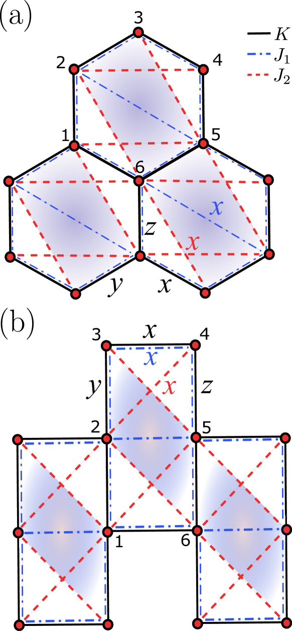
Figure 1: The Kitaev-Ising-$J_{1}$-$J_{2}$ model on the hexagonal (a) and square (b) lattices. Black lines represent the pure Kitaev model coupling $K$, blue dashed lines with dots indicate to the NN XX coupling $J_{1}$, and red dashed lines denote to the NNN XX coupling $J_{2}$. Shaded sectors denote the sites involved in the calculation of magnetic order parameters (6),(7).

II.2 Density Matrix Renormalization Group

Here, we briefly summarize the key aspects of the DMRG method and the MPS ansatz. For a more comprehensive discussion, see [58, 59, 60, 61].

Consider a spin-$\frac{1}{2}$ lattice with $N$ sites, with each site described by a basis of spin-up/spin-down states $\left\{\left|\uparrow\right>,\left|\downarrow\right>\right\}$. The many-body wave function of the system is given by

$$\left|\psi\right>=\sum_{i_{1}i_{2}...i_{N}}\psi^{i_{1}i_{2}..i_{N}}\left|i_{1}i_{2}...i_{N}\right>,$$ (8)

where $\psi^{i_{1}i_{2}..i_{N}}$ represents $2^{N}$ complex amplitudes and $\left|i_{1}i_{2}...i_{N}\right>$ stands for the product basis $\left|i_{1}\right>\otimes\left|i_{2}\right>\otimes\dotsm\otimes\left|i_{N}\right>$ for $2^{N}$-dimensional vector space of the $N$ sites. Similarly, the local many-body Hamiltonian in this basis is expressed as

$$\mathcal{H}=\sum_{\left\{i\right\},\left\{j\right\}}\mathcal{H}^{i_{1}j_{1}i_{2}j_{2}..i_{N}j_{N}}\left|i_{1}i_{2}...i_{N}\right>\left<j_{1}j_{2}...j_{N}\right|.$$ (9)

Our goal is to compute an accurate approximation of the ground state $\left|\psi_{\text{GS}}\right>$ of the Hamiltonian $\mathcal{H}$. One can use the exact diagonalization method, but we are limited to small systems, because the dimension of the Hilbert space (8) grows exponentially with the system size $N$. This limitation is known as the exponential wall problem[62]. To overcome this challenge, we require a computational method that avoids the need to explicitly store the full wave function (8) amplitudes.

One of the numerical methods that allows bypassing the exponential wall problem is DMRG [44, 45]. This algorithm has its roots in Wilson’s numerical renormalization group [63, 64], whose key idea is to divide a large quantum system into smaller blocks that can be solved by exact diagonalization. This algorithm is not very effective for strongly correlated systems [45].

In the DMRG method the truncation procedure is more accurate than in previous approaches, because the basis is rotated such that only a small number of states are required to represent the ground state, while the remaining states can be discarded. To improve efficiency, basis rotations are performed iteratively on a few sites at a time, treating the remaining sites as an environment. This iterative sweeping process enables global basis optimization across all lattice sites without requiring a full Hilbert space transformation in a single step. As a result, the variational algorithm produces a wave function expressed in a compact form known as the matrix product state (MPS) [65]. The modern formulation of DMRG is built upon tensor networks, where the algorithm begins with an MPS as a variational ansatz and then optimizes all its coefficients [47, 66, 58].

The computational cost of optimizing MPS from site $n$ to site $n+1$ is $O(D^{3})$, resulting in a total optimization sweep cost that scales as $O(ND^{3})$, where $D$ is the bond dimension and $N$ is the system size. For a generic (nonlocal) Hamiltonian (9) bond dimension $D$ grows exponentially with the entanglement entropy, following $D\sim\exp{\left(S\right)}$ [50, 67]. Simultaneously, the entanglement entropy obeys a scaling law known as the volume law, where $S\sim N$. Consequently, in the generic case, the bond dimension scales exponentially with system size as $D\sim\exp{\left(N\right)}$.

A key factor in the success of DMRG is the area law: the ground state of many physical systems can often be accurately represented by an MPS with a fixed bond dimension $D$ [50, 49, 68, 52, 69]. This implies that the entanglement entropy $S$, rather than being an extensive quantity, is at most proportional to the boundary of the bipartition. For the ground state of a local Hamiltonian (9) describing a $d$-dimensional system of linear size $L$ made of $N=L^{d}$ sites, the entanglement entropy scales as

$$S\sim L^{d-1}=N^{\left(d-1\right)/d},$$ (10)

$$D\sim\exp{\left(L^{d-1}\right)}=\exp{\left(N^{\left(d-1\right)/d}\right)}.$$ (11)

In one dimension ($d=1$), the entanglement entropy remains constant $S\sim\operatorname{const}$ for gapped systems, implying that the bond dimension $D$ is also constant and independent of system size $N$. Consequently, the computational cost for a $1D$ scales as $O(N)$. For 1D gapless/critical models, the entanglement entropy follows a logarithmic scaling with system size $S\sim\operatorname{ln}{(N)}$, leading to a polynomially growing bond dimension $D\sim\operatorname{poly}{(N)}$. This behavior is known as the logarithmic correction to the area law [50].

In higher dimensions ($d=2,3$) the computational complexity increases significantly. While the system still obeys the area law, the bond dimension grows exponentially with the system size as $\exp{(\sqrt{N})}$ and $\exp{(N^{2/3})}$ for $d=2,3$. Nevertheless, DMRG remains advantageous, as its computational cost scales as a fractional power of $N$, in contrast to the $\exp{(N)}$ scaling of brute-force computation methods, which suffer from the exponential wall problem [62].

In conclusion, DMRG is a highly effective computational method that has become dominant in the study of strongly correlated 1D systems. Despite its unfavorable scaling in higher dimensions, DMRG remains widely used for 2D systems, particularly when one dimension is relatively small, as in stripe and cylindrical geometries [70, 71, 72, 73] (for a review of 2D DMRG, see [59]). Additionally, DMRG has been successfully applied to small 3D molecular systems [74, 75, 76, 77, 78].

III Numerical results

In this section, we present the numerical results for the Kitaev-Ising-$J_{1}$-$J_{2}$ model (II.1) obtained using DMRG simulations. In particular, we determine the ground-state phase diagram of the system on a $10\times 10$ square lattice with $N=100$ sites and with the periodic boundary conditions along $x$-axis and open boundary condition along $y$-axis (Sec. III.1). We compute the entanglement entropy and the maximum bond dimension as functions of system size (Sec.III.2). Additionally, we introduce an analog of adiabatic quantum optimization for DMRG to prevent getting stuck in the local minima and reach a global energy minimum (Sec. III.3). DMRG simulations were performed with a truncation error less than $10^{-9}$, the Krylov dimension is 5, and the number of sweeps is 35. All calculations were carried out using our proposed optimization algorithm (see Sec. III.3).

III.1 Quantum phase diagram

We calculate the order parameters $\sigma_{\text{I}}$ (6), $\sigma_{\text{II}}$ (7), and topological order parameter $W_{p}=2^{6}S^{x}_{1}S^{y}_{2}S^{z}_{3}S^{x}_{4}S^{y}_{5}S^{z}_{6}$, as introduced in Sec. II.1 and summarized in Tab. 1. The order parameters $\sigma_{\text{I}}$ and $\sigma_{\text{II}}$ indicate the presence of a magnetic order, whereas $W_{p}$ characterizes the topological order. As shown in Fig. 2, the ground state hosts seven distinct phases: four with commensurate order (FM, Neel, x- and y-stripy), two with incommensurate order (labelled IC1 and IC2), and KSL phase. We also calculate the static spin-structure factor

$$S(\mathbf{k})=\frac{1}{N}\sum_{ij}\left(\left<S^{x}_{i}S^{x}_{j}\right>+\left<S^{y}_{i}S^{y}_{j}\right>+\left<S^{z}_{i}S^{z}_{j}\right>\right)e^{i\mathbf{k}\left(\mathbf{r}_{i}-\mathbf{r}_{j}\right)},$$ (12)

where $N$ is the number of sites, and $\mathbf{r}_{i}$ denotes the position of the site $i$.

Spin-structure factor characterizes the spin-spin correlations in the system. In Fig. 3 the Bragg peaks corresponding to the $\left<\mathbf{S}_{i}\mathbf{S}_{j}\right>$ correlations are plotted in the extended Brillouin zone. For commensurate (ordered) magnetic phases, the Bragg peak positions reflect the underlying lattice symmetry. In contrast, in the incommensurate phase, the Bragg peaks are shifted and do not follow the lattice symmetry. Thus, the magnetic structure can be inferred from the Bragg peak positions in reciprocal space. Additionally, we note that the spin-structure factor can provide insight into the system’s entanglement properties [79], which we discuss in Sec. IV.

III.1.1 Kitaev Spin Liquid state

As mentioned in Sec. II.1, our model includes the Kitaev term (1), which gives rise to either a gapped or gapless KSL state. For simplicity, we assume that $J_{x}=J_{y}=J_{z}=K$ in the Kitaev term (1), corresponding to the gapless KSL phase. In this phase, the magnetic order parameters (6) and (7) vanish (see Tab. 1), but there is a topological order parameter $W_{p}=2^{6}S^{x}_{1}S^{y}_{2}S^{z}_{3}S^{x}_{4}S^{y}_{5}S^{z}_{6}$ (see Fig. 1) remains nontrivial. This parameter takes the value $W_{p}=1$ in the KSL state.

The KSL state exists within a narrow range of parameters near the Kitaev points $\varphi=\{0,\pi,2\pi\}$. This result is expected, as a similar phase structure is typical in spin models with Kitaev interactions, such as the Kitaev-Heisenberg model [80, 81], the $K_{1}$-$K_{2}$ model [34], and the Kitaev-Heisenberg-Gamma model (or J-K-$\Gamma$ model) [23, 26].

As shown in Fig. 3, two distinct spin liquid phases emerge near the Kitaev points, depending on the sign of the Kitaev interaction coupling constant $K=\cos{\varphi}$. For $K>0$, the system enters the ferromagnetic Kitaev spin liquid (FM KSL) phase (see Fig. 3a), characterized by a soft peak at the $\Gamma$-point. Conversely, for $K<0$, the system realizes the antiferromagnetic Kitaev spin liquid (AFM KSL) phase (see Fig. 3b), where the spin-structure factor exhibits broad maxima around the K-points of the first Brillouin zone (BZ), analogous to the FM KSL phase. In both regimes, the KSL phase is marked by delocalized Bragg peaks in the spin-spin correlations (see Fig. 3(a-b)), which may indicate strong quantum entanglement (see Sec. IV). Throughout this work, we refer to both phases as KSL, as they share the same fundamental properties.

III.1.2 Commensurate magnetic phases

Well-known phases in frustrated magnetic models are commensurate magnetic phases such as FM, Neel, x-stripy, and y-stripy (see Fig. 2 and Fig. 3). In this work, we refer to the phases as x-stripy and y-stripy in the context of the honeycomb model mapped to the square lattice, as this notation aligns more naturally with the spin configuration shown in real space in Fig. 2. However, for the honeycomb lattice, the $y$-stripy phase is more commonly referred to as the zigzag phase.

As summarized in Tab. 1, the topological order parameter vanishes in all magnetic phases, while each magnetic phase exhibits a distinct value of the order parameters (6) or (7). The Bragg peaks of the spin-spin correlations are localized and preserve the honeycomb lattice symmetry in the reciprocal space (see Fig. 3(e-h)). This localization may indicate low entanglement in these phases (see Sec. IV).

III.1.3 Incommensurate magnetic phases

Another notable regime in this model is the incommensurate magnetic phase, which, unlike commensurate phases, lacks periodicity matching that of the original lattice (up to the nearest rational number). Such phases are characteristic of Kitaev models with symmetric off-diagonal anisotropic $\Gamma$ interactions, as seen in the Heisenberg-Kitaev-$\Gamma$ model [26, 27, 28, 29, 30, 31, 32, 33]. Variants of this ordering have been shown to emerge in models dominated by strong Kitaev exchange with additional weaker isotropic $J$ exchange [82, 28]. In contrast, our model contains only diagonal anisotropic interactions (Kitaev and Ising $J_{1}$, $J_{2}$) and lacks both $\Gamma$- and $J$-like interactions.

The incommensurate state lacks topological order ($W_{p}=0$) and have spatially modulated order parameters (see Tab. 1). These phases stabilize near the Kitaev limits and exhibit a zero average magnetic moment at each lattice site. The first incommensurate phase (IC1, see Fig. 2 and Fig. 3c) is incommensurate along the $\mathbf{b_{1}}=\frac{2\pi}{3}(\sqrt{3},1)$ direction. The second incommensurate phase (IC2, see Fig. 2 and Fig. 3d) is incommensurate along both reciprocal lattice basis vectors $\mathbf{b_{1}}$ and $\mathbf{b_{2}}=\frac{4\pi}{3}(1,0)$. Both incommensurate phases are highly degenerate and frustrated, which leads to strong entanglement comparable to the entanglement in the KSL state (see Fig. 4) [83]. The Bragg peaks of the spin-spin correlations are partially delocalized and shifted (see Fig. 3(c-d)), indicating incommensurate magnetic order. Note that this partial delocalization may serve as a signature of a highly entangled state (see Sec. IV).

Table 1: Order parameters and entanglement entropy for all possible phases in the Kitaev-Ising-$J_{1}$-$J_{2}$ model.

Phase	$W_{p}$	$\sigma_{\text{I}}$	$\sigma_{\text{II}}$	$S$
KSL	1	0	0	$\sim\sqrt{N}$
IC1	0	$-0.1\div-0.4$	$0.1\div 0.4$	$\sim\sqrt{N}$
IC2	0	$0.1\div 0.4$	$-0.1\div-0.4$	$\sim\sqrt{N}$
FM	0	1	0	$\sim\operatorname{const}$
x-stripy	0	-1	0	$\sim\operatorname{const}$
Neel	0	0	1	$\sim\operatorname{const}$
y-stripy	0	0	-1	$\sim\operatorname{const}$

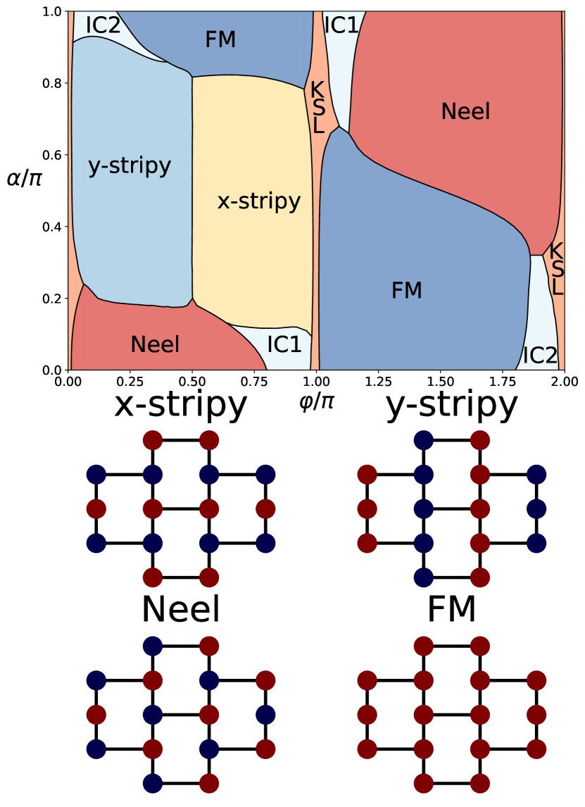
Figure 2: Phase diagram of the Kitaev-Ising-$J_{1}$-$J_{2}$ model, along with schematic spin configurations for commensurate phases. Red (blue) points represent spin-up (spin-down) states with $\left<S^{x}\right>=+1/2$ ($\left<S^{x}\right>=-1/2$).

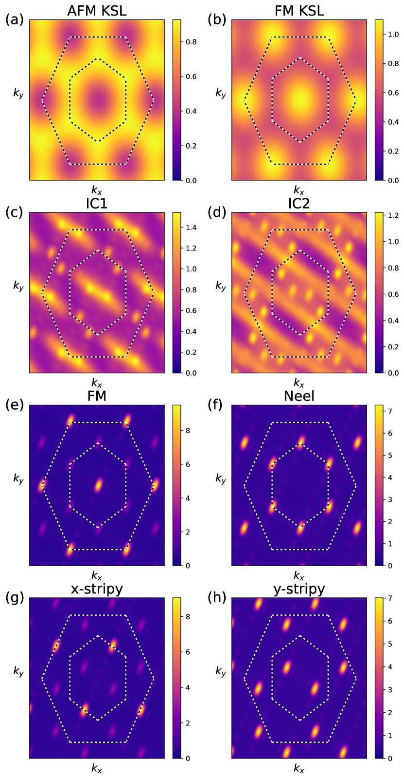
Figure 3: Spin-structure factor $S(\mathbf{k})$ of the Kitaev-Ising-$J_{1}$-$J_{2}$ model for representative momenta in different phases. The larger black and white dashed hexagone denotes the extended Brillouin zone, while the inner hexagone represents the first Brilloin zone. (a) AFM KSL phase, plotted at $\alpha=0,\,\,\varphi=0$. (b) FM KSL phase at $\alpha=0,\,\,\varphi=\pi$. (c) FM phase at $\alpha=0,\,\,\varphi=1.5\pi$. (d) Neel phase $\alpha=0,\,\,\varphi=0.5\pi$. (e) x-stripy phase at $\alpha=0.5\pi,\,\,\varphi=0.75\pi$. (f) y-stripy phase at $\alpha=0.5\pi,\,\,\varphi=0.25\pi$. (g) IC1 phase at $\alpha=0,\,\,\varphi=0.85\pi$. (h) IC2 phase at $\alpha=0,\,\,\varphi=1.85\pi$.

III.2 Entanglement entropy and bond dimension

In this section, we analyze the entanglement entropy and the maximum bond dimension across different phases. These quantities are plotted in Fig. 4 as functions of system size.

The most entangled phases are the KSL and the incommensurate magnetic phases IC1 and IC2 (see Tab. 1 and Fig. 4). In these phases, the entanglement entropy $S$ scales as $\sqrt{N}$, leading to an exponentially growing bond dimension $D\sim e^{\sqrt{N}}$, in accordance with the area law. Interestingly, incommensurate phases exhibit the same exponential scaling, a behavior typically associated with the KSL state [84, 85]. Since the MPS representation grows exponentially with system size, more advanced wave function ansätze, such as projected entangled pair states (PEPS) and the multiscale entanglement renormalization ansatz (MERA), are required for efficient simulations in 2D. Notably, despite its exponential scaling, this approach remains significantly more efficient than brute-force methods, which scale as $e^{N}$.

Commensurate magnetic phases have a near-zero entanglement entropy value,see Fig. 4, resulting in a constant bond dimension $D$. In practice, this implies that these low-entanglement magnetic phases are well described by mean-field theory, requiring only a small bond dimension to accurately capture the MPS representation. After the first sweep, the MPS is already well-converged. However, this scenario presents a challenge: in our system, the DMRG algorithm tends to become trapped in local minima.

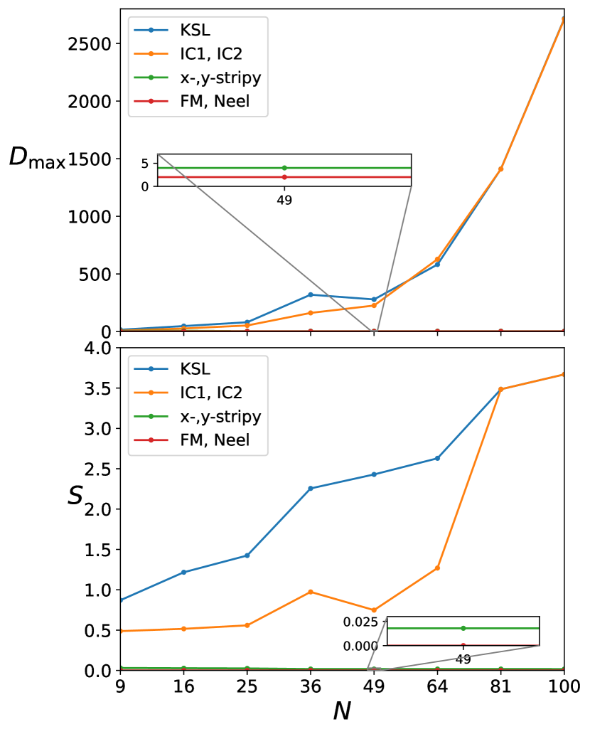
Figure 4: Scaling of the entanglement entropy (top) and the maximum bond dimension (bottom) with system size. The calculations for different phases were performed at the same values of $\alpha$ and $\varphi$ as in the Fig. 3. The lattice size $N$ varies from $3\times 3$ to $10\times 10$.

III.3 Optimization algorithm for ground state energy

In low-entanglement phases, the DMRG method encounters a convergence issue —- the ground state energy fails to stabilize (see the blue line in Fig. 5). Potential solutions, such as introducing a noise term, increasing the dimension of the Krylov subspace, or extending the number of Krylov subspace rebuilds, either prove ineffective or further exacerbate the problem.

Here, we propose an algorithm to efficiently determine the ground state energy. We introduce the following modified Hamiltonian

$$H(\lambda)=\left(1-\lambda\right)H_{0}+\lambda H^{\prime},$$ (13)

where $\lambda$ is the weight parameter, the $H_{0}$ is the origin Hamiltonian (II.1), and the $\lambda H^{\prime}$ represents a perturbation term. We consider the following perturbation term

$$H^{\prime}=\sum_{i}\mathbf{B}\cdot\mathbf{S}_{i},$$ (14)

where $B$ is a magnitude of an applied magnetic field. In our algorithm, we set $B=(0,0,B_{\text{z}})$. Notably, the optimization procedure remains effective for any choice of magnetic field direction in the perturbation term (14).

Now we are ready to perform the optimization algorithm, which has the following structure. In the first step, we set $\lambda=1$ in the Hamiltonian (13) and perform a DMRG routine to obtain the optimized wave function $\left|\psi_{\lambda=1}\right>$. We use $\left|\psi_{\lambda=1}\right>$ as an initial in the next step, where we gradually (adiabatically) ”turn off” the perturbation term by reducing the weight parameter $\lambda$ by a small $\varepsilon$ and after DMRG procedure we get a new optimized wave function $\left|\psi_{\lambda=1-\varepsilon}\right>$. Then we repeat this process until $\lambda=0$. In the final step, we perform the DMRG for original Hamiltonian (II.1), using $\left|\psi_{\lambda=0}\right>$ as the initial wave function, to obtain the optimized ground state.

In Fig. 5 is shown the result of performing optimization algorithm, where the ground state energy is plotted with the respect to the parameter $\varphi$. As was written before, in the low entangled phase MPS is getting stuck. This occurs because commensurate magnetic phases (low entanglement states) are well described by a mean-field ansatz, resulting in a fixed bond dimension for each DMRG sweep. Consequently, the bond dimension cannot gradually increase, as the MPS becomes stuck in a low-energy state without reaching the true ground state. Our optimization algorithm addresses this issue by preparing the MPS in a controlled manner, ensuring that it converges directly to the ground state.

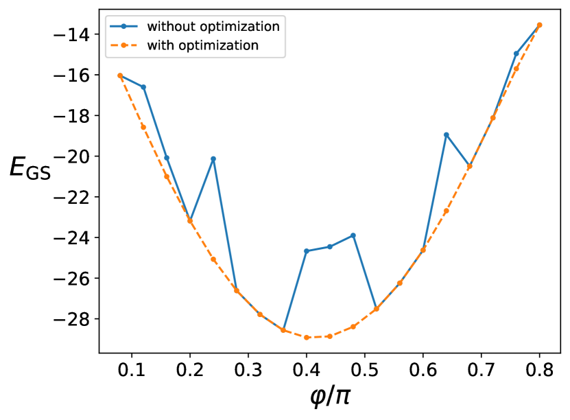
Figure 5: Results of the optimization algorithm for $\varphi/\pi\in\left[0.1,0.8\right]$ and $\alpha=0$. The optimization procedure is effective across the entire parameter range of $\varphi$ and $\alpha$. The blue line represents the case without optimization, while the dashed orange line shows the ground-state energy obtained with optimization.

IV Discussion

In this article, we investigate the Kitaev honeycomb model with the additional XX Ising interaction between the nearest and the next nearest neighbors (Kitaev-Ising-$J_{1}$-$J_{2}$ model). Using DMRG, we determine the ground state of the system, which hosts low entangled commensurate magnetic phases and entangled KSL and incommensurate phases. We show that anisotropic Ising interactions can stabilize incommensurate phases, previously thought to require more complex interactions. We analyze the scaling behavior of entanglement entropy and the bond dimension of the matrix product state, and we propose an optimization algorithm to improve DMRG convergence in low entangled phases.

As we mentioned in the Sec. III.1, high entangled phases (such as KSL, IC1, and IC2) have a delocalized spin-structure factor. This indicates not only that the spin-spin correlations in the system are incommensurate with the lattice, but is also an measure of the entanglement of the system. In the Ref. [79], is considered the quantity $E(\mathbf{q})=\operatorname{max}\{0,1-\frac{1}{2}S(\mathbf{q})\}$, which provides a lower bound to the many-particle entanglement (as measured in terms of the best separable approximation) contained in the system, and $\operatorname{min}\{E(\mathbf{q})\}$ shows the minimum possible entanglement in the system. We found that $\operatorname{min}\{E(\mathbf{q})\}=0$ in the low entangled phases (FM, Neel, x-, and y-stripy) and $\operatorname{min}\{E(\mathbf{q})\}\neq 0$ in the high entangled phases (KSL, IC1, and IC2). This correlates with our results and suggests that delocalization of the spin-structure factor leads to the appearance of entanglement in the system.

References

- Balents [2010] L. Balents, Spin liquids in frustrated magnets, Nature 464, 199 (2010).
- Savary and Balents [2016] L. Savary and L. Balents, Quantum spin liquids: a review, Reports on Progress in Physics 80, 016502 (2016).
- Zhou et al. [2017a] Y. Zhou, K. Kanoda, and T.-K. Ng, Quantum spin liquid states, Rev. Mod. Phys. 89, 025003 (2017a).
- Wen et al. [2019] J. Wen, S.-L. Yu, S. Li, W. Yu, and J.-X. Li, Experimental identification of quantum spin liquids, npj Quantum Materials 4, 12 (2019).
- Broholm et al. [2020] C. Broholm, R. J. Cava, S. A. Kivelson, D. G. Nocera, M. R. Norman, and T. Senthil, Quantum spin liquids, Science 367, eaay0668 (2020).
- Wen [1991] X. G. Wen, Mean-field theory of spin-liquid states with finite energy gap and topological orders, Phys. Rev. B 44, 2664 (1991).
- Wen [2013] X.-G. Wen, Topological order: From long-range entangled quantum matter to a unified origin of light and electrons, ISRN Condensed Matter Physics 2013, 198710 (2013).
- Senthil and Fisher [2000] T. Senthil and M. P. A. Fisher, gauge theory of electron fractionalization in strongly correlated systems, Phys. Rev. B 62, 7850 (2000).
- Senthil and Fisher [2001] T. Senthil and M. P. A. Fisher, Fractionalization in the cuprates: Detecting the topological order, Phys. Rev. Lett. 86, 292 (2001).
- Read and Sachdev [1991] N. Read and S. Sachdev, Large-n expansion for frustrated quantum antiferromagnets, Phys. Rev. Lett. 66, 1773 (1991).
- Sachdev [1992] S. Sachdev, Kagome´- and triangular-lattice heisenberg antiferromagnets: Ordering from quantum fluctuations and quantum-disordered ground states with unconfined bosonic spinons, Phys. Rev. B 45, 12377 (1992).
- Lee et al. [2006] P. A. Lee, N. Nagaosa, and X.-G. Wen, Doping a mott insulator: Physics of high-temperature superconductivity, Rev. Mod. Phys. 78, 17 (2006).
- Kitaev [2006] A. Kitaev, Anyons in an exactly solved model and beyond, Annals of Physics 321, 2 (2006).
- Zhou et al. [2017b] Y. Zhou, K. Kanoda, and T.-K. Ng, Quantum spin liquid states, Rev. Mod. Phys. 89, 025003 (2017b).
- Jackeli and Khaliullin [2009] G. Jackeli and G. Khaliullin, Mott insulators in the strong spin-orbit coupling limit: From heisenberg to a quantum compass and kitaev models, Phys. Rev. Lett. 102, 017205 (2009).
- Plumb et al. [2014] K. W. Plumb, J. P. Clancy, L. J. Sandilands, V. V. Shankar, Y. F. Hu, K. S. Burch, H.-Y. Kee, and Y.-J. Kim, : A spin-orbit assisted mott insulator on a honeycomb lattice, Phys. Rev. B 90, 041112 (2014).
- Yokoi et al. [2021] T. Yokoi, S. Ma, Y. Kasahara, S. Kasahara, T. Shibauchi, N. Kurita, H. Tanaka, J. Nasu, Y. Motome, C. Hickey, et al., Half-integer quantized anomalous thermal hall effect in the kitaev material candidate -rucl3, Science 373, 568 (2021).
- Banerjee et al. [2022] S. Banerjee, U. Kumar, and S.-Z. Lin, Inverse faraday effect in mott insulators, Phys. Rev. B 105, L180414 (2022).
- Bruin et al. [2022] J. A. N. Bruin, R. R. Claus, Y. Matsumoto, N. Kurita, H. Tanaka, and H. Takagi, Robustness of the thermal hall effect close to half-quantization in -rucl3, Nature Physics 18, 401 (2022).
- Trebst and Hickey [2022] S. Trebst and C. Hickey, Kitaev materials, Physics Reports 950, 1 (2022).
- Nica et al. [2023] E. M. Nica, M. Akram, A. Vijayvargia, R. Moessner, and O. Erten, Kitaev spin-orbital bilayers and their moiré superlattices, npj Quantum Materials 8, 9 (2023).
- Chaloupka et al. [2010] J. c. v. Chaloupka, G. Jackeli, and G. Khaliullin, Kitaev-heisenberg model on a honeycomb lattice: Possible exotic phases in iridium oxides , Phys. Rev. Lett. 105, 027204 (2010).
- Chaloupka et al. [2013] J. c. v. Chaloupka, G. Jackeli, and G. Khaliullin, Zigzag magnetic order in the iridium oxide , Phys. Rev. Lett. 110, 097204 (2013).
- Yamaji et al. [2016] Y. Yamaji, T. Suzuki, T. Yamada, S.-i. Suga, N. Kawashima, and M. Imada, Clues and criteria for designing a kitaev spin liquid revealed by thermal and spin excitations of the honeycomb iridate , Phys. Rev. B 93, 174425 (2016).
- Gotfryd et al. [2017] D. Gotfryd, J. Rusnačko, K. Wohlfeld, G. Jackeli, J. c. v. Chaloupka, and A. M. Oleś, Phase diagram and spin correlations of the kitaev-heisenberg model: Importance of quantum effects, Phys. Rev. B 95, 024426 (2017).
- Rau et al. [2014] J. G. Rau, E. K.-H. Lee, and H.-Y. Kee, Generic spin model for the honeycomb iridates beyond the kitaev limit, Phys. Rev. Lett. 112, 077204 (2014).
- Chaloupka and Khaliullin [2015] J. c. v. Chaloupka and G. Khaliullin, Hidden symmetries of the extended kitaev-heisenberg model: Implications for the honeycomb-lattice iridates , Phys. Rev. B 92, 024413 (2015).
- Lee and Kim [2015] E. K.-H. Lee and Y. B. Kim, Theory of magnetic phase diagrams in hyperhoneycomb and harmonic-honeycomb iridates, Phys. Rev. B 91, 064407 (2015).
- Yadav et al. [2016] R. Yadav, N. A. Bogdanov, V. M. Katukuri, S. Nishimoto, J. van den Brink, and L. Hozoi, Kitaev exchange and field-induced quantum spin-liquid states in honeycomb -rucl3, Scientific Reports 6, 37925 (2016).
- Nishimoto et al. [2016] S. Nishimoto, V. M. Katukuri, V. Yushankhai, H. Stoll, U. K. Rößler, L. Hozoi, I. Rousochatzakis, and J. van den Brink, Strongly frustrated triangular spin lattice emerging from triplet dimer formation in honeycomb li2iro3, Nature Communications 7, 10273 (2016).
- Yadav et al. [2019] R. Yadav, S. Nishimoto, M. Richter, J. van den Brink, and R. Ray, Large off-diagonal exchange couplings and spin liquid states in -symmetric iridates, Phys. Rev. B 100, 144422 (2019).
- Zhang et al. [2021] S.-S. Zhang, G. B. Halász, W. Zhu, and C. D. Batista, Variational study of the kitaev-heisenberg-gamma model, Phys. Rev. B 104, 014411 (2021).
- Buessen and Kim [2021] F. L. Buessen and Y. B. Kim, Functional renormalization group study of the kitaev- model on the honeycomb lattice and emergent incommensurate magnetic correlations, Phys. Rev. B 103, 184407 (2021).
- Rousochatzakis et al. [2015] I. Rousochatzakis, J. Reuther, R. Thomale, S. Rachel, and N. B. Perkins, Phase diagram and quantum order by disorder in the kitaev honeycomb magnet, Phys. Rev. X 5, 041035 (2015).
- Kimchi and You [2011] I. Kimchi and Y.-Z. You, Kitaev-heisenberg-- model for the iridates iro3, Phys. Rev. B 84, 180407 (2011).
- Sizyuk et al. [2014] Y. Sizyuk, C. Price, P. Wölfle, and N. B. Perkins, Importance of anisotropic exchange interactions in honeycomb iridates: Minimal model for zigzag antiferromagnetic order in , Phys. Rev. B 90, 155126 (2014).
- Buluta and Nori [2009] I. Buluta and F. Nori, Quantum simulators, Science 326, 108 (2009).
- Altman et al. [2021] E. Altman, K. R. Brown, G. Carleo, L. D. Carr, E. Demler, C. Chin, B. DeMarco, S. E. Economou, M. A. Eriksson, K.-M. C. Fu, M. Greiner, K. R. Hazzard, R. G. Hulet, A. J. Kollár, B. L. Lev, M. D. Lukin, R. Ma, X. Mi, S. Misra, C. Monroe, K. Murch, Z. Nazario, K.-K. Ni, A. C. Potter, P. Roushan, M. Saffman, M. Schleier-Smith, I. Siddiqi, R. Simmonds, M. Singh, I. Spielman, K. Temme, D. S. Weiss, J. Vučković, V. Vuletić, J. Ye, and M. Zwierlein, Quantum simulators: Architectures and opportunities, PRX Quantum 2, 017003 (2021).
- Semeghini et al. [2021] G. Semeghini, H. Levine, A. Keesling, S. Ebadi, T. T. Wang, D. Bluvstein, R. Verresen, H. Pichler, M. Kalinowski, R. Samajdar, et al., Probing topological spin liquids on a programmable quantum simulator, Science 374, 1242 (2021).
- Satzinger et al. [2021] K. J. Satzinger, Y.-J. Liu, A. Smith, C. Knapp, M. Newman, C. Jones, Z. Chen, C. Quintana, X. Mi, A. Dunsworth, C. Gidney, I. Aleiner, F. Arute, K. Arya, J. Atalaya, R. Babbush, J. C. Bardin, R. Barends, J. Basso, A. Bengtsson, A. Bilmes, M. Broughton, B. B. Buckley, D. A. Buell, B. Burkett, N. Bushnell, B. Chiaro, R. Collins, W. Courtney, S. Demura, A. R. Derk, D. Eppens, C. Erickson, L. Faoro, E. Farhi, A. G. Fowler, B. Foxen, M. Giustina, A. Greene, J. A. Gross, M. P. Harrigan, S. D. Harrington, J. Hilton, S. Hong, T. Huang, W. J. Huggins, L. B. Ioffe, S. V. Isakov, E. Jeffrey, Z. Jiang, D. Kafri, K. Kechedzhi, T. Khattar, S. Kim, P. V. Klimov, A. N. Korotkov, F. Kostritsa, D. Landhuis, P. Laptev, A. Locharla, E. Lucero, O. Martin, J. R. McClean, M. McEwen, K. C. Miao, M. Mohseni, S. Montazeri, W. Mruczkiewicz, J. Mutus, O. Naaman, M. Neeley, C. Neill, M. Y. Niu, T. E. O’Brien, A. Opremcak, B. Pató, A. Petukhov, N. C. Rubin, D. Sank, V. Shvarts, D. Strain, M. Szalay, B. Villalonga, T. C. White, Z. Yao, P. Yeh, J. Yoo, A. Zalcman, H. Neven, S. Boixo, A. Megrant, Y. Chen, J. Kelly, V. Smelyanskiy, A. Kitaev, M. Knap, F. Pollmann, and P. Roushan, Realizing topologically ordered states on a quantum processor, Science 374, 1237 (2021).
- Krantz et al. [2019] P. Krantz, M. Kjaergaard, F. Yan, T. P. Orlando, S. Gustavsson, and W. D. Oliver, A quantum engineer’s guide to superconducting qubits, Applied Physics Reviews 6, 021318 (2019), https://pubs.aip.org/aip/apr/article-pdf/doi/10.1063/1.5089550/16667201/021318_1_online.pdf .
- Yan et al. [2018] F. Yan, P. Krantz, Y. Sung, M. Kjaergaard, D. L. Campbell, T. P. Orlando, S. Gustavsson, and W. D. Oliver, Tunable coupling scheme for implementing high-fidelity two-qubit gates, Phys. Rev. Appl. 10, 054062 (2018).
- Sung et al. [2021] Y. Sung, L. Ding, J. Braumüller, A. Vepsäläinen, B. Kannan, M. Kjaergaard, A. Greene, G. O. Samach, C. McNally, D. Kim, A. Melville, B. M. Niedzielski, M. E. Schwartz, J. L. Yoder, T. P. Orlando, S. Gustavsson, and W. D. Oliver, Realization of high-fidelity cz and -free iswap gates with a tunable coupler, Phys. Rev. X 11, 021058 (2021).
- White [1992] S. R. White, Density matrix formulation for quantum renormalization groups, Phys. Rev. Lett. 69, 2863 (1992).
- White [1993] S. R. White, Density-matrix algorithms for quantum renormalization groups, Phys. Rev. B 48, 10345 (1993).
- Affleck et al. [1987] I. Affleck, T. Kennedy, E. H. Lieb, and H. Tasaki, Rigorous results on valence-bond ground states in antiferromagnets, Phys. Rev. Lett. 59, 799 (1987).
- Östlund and Rommer [1995] S. Östlund and S. Rommer, Thermodynamic limit of density matrix renormalization, Phys. Rev. Lett. 75, 3537 (1995).
- Rommer and Östlund [1997] S. Rommer and S. Östlund, Class of ansatz wave functions for one-dimensional spin systems and their relation to the density matrix renormalization group, Phys. Rev. B 55, 2164 (1997).
- Srednicki [1993] M. Srednicki, Entropy and area, Phys. Rev. Lett. 71, 666 (1993).
- Vidal et al. [2003] G. Vidal, J. I. Latorre, E. Rico, and A. Kitaev, Entanglement in quantum critical phenomena, Phys. Rev. Lett. 90, 227902 (2003).
- Gioev and Klich [2006] D. Gioev and I. Klich, Entanglement entropy of fermions in any dimension and the widom conjecture, Phys. Rev. Lett. 96, 100503 (2006).
- Amico et al. [2008] L. Amico, R. Fazio, A. Osterloh, and V. Vedral, Entanglement in many-body systems, Rev. Mod. Phys. 80, 517 (2008).
- Winter et al. [2017] S. M. Winter, A. A. Tsirlin, M. Daghofer, J. van den Brink, Y. Singh, P. Gegenwart, and R. Valentí, Models and materials for generalized kitaev magnetism, Journal of Physics: Condensed Matter 29, 493002 (2017).
- Rousochatzakis et al. [2024] I. Rousochatzakis, N. B. Perkins, Q. Luo, and H.-Y. Kee, Beyond kitaev physics in strong spin-orbit coupled magnets, Reports on Progress in Physics 87, 026502 (2024).
- Hermanns et al. [2018] M. Hermanns, I. Kimchi, and J. Knolle, Physics of the kitaev model: Fractionalization, dynamic correlations, and material connections, Annual Review of Condensed Matter Physics 9, 17 (2018).
- Abalmasov and Vugmeister [2023] V. A. Abalmasov and B. E. Vugmeister, Metastable states in the ising model, Phys. Rev. E 107, 034124 (2023).
- Karimipour et al. [2013] V. Karimipour, L. Memarzadeh, and P. Zarkeshian, Kitaev-ising model and the transition between topological and ferromagnetic order, Phys. Rev. A 87, 032322 (2013).
- Schollwöck [2011] U. Schollwöck, The density-matrix renormalization group in the age of matrix product states, Annals of Physics 326, 96 (2011), january 2011 Special Issue.
- Stoudenmire and White [2012] E. Stoudenmire and S. R. White, Studying two-dimensional systems with the density matrix renormalization group, Annual Review of Condensed Matter Physics 3, 111 (2012).
- Catarina and Murta [2023] G. Catarina and B. Murta, Density-matrix renormalization group: a pedagogical introduction, The European Physical Journal B 96, 111 (2023).
- Ganahl et al. [2023] M. Ganahl, J. Beall, M. Hauru, A. G. Lewis, T. Wojno, J. H. Yoo, Y. Zou, and G. Vidal, Density matrix renormalization group with tensor processing units, PRX Quantum 4, 010317 (2023).
- Kohn [1999] W. Kohn, Nobel lecture: Electronic structure of matter—wave functions and density functionals, Rev. Mod. Phys. 71, 1253 (1999).
- Wilson [1975] K. G. Wilson, The renormalization group: Critical phenomena and the kondo problem, Rev. Mod. Phys. 47, 773 (1975).
- Bulla et al. [2008] R. Bulla, T. A. Costi, and T. Pruschke, Numerical renormalization group method for quantum impurity systems, Rev. Mod. Phys. 80, 395 (2008).
- Fannes et al. [1992] M. Fannes, B. Nachtergaele, and R. F. Werner, Finitely correlated states on quantum spin chains, Communications in Mathematical Physics 144, 443 (1992).
- Dukelsky et al. [1998] J. Dukelsky, M. A. Martín-Delgado, T. Nishino, and G. Sierra, Equivalence of the variational matrix product method and the density matrix renormalization group applied to spin chains, Europhysics Letters 43, 457 (1998).
- Peschel [2003] I. Peschel, Calculation of reduced density matrices from correlation functions, Journal of Physics A: Mathematical and General 36, L205 (2003).
- Hastings [2007] M. B. Hastings, An area law for one-dimensional quantum systems, Journal of Statistical Mechanics: Theory and Experiment 2007, P08024 (2007).
- Eisert et al. [2010] J. Eisert, M. Cramer, and M. B. Plenio, Colloquium: Area laws for the entanglement entropy, Rev. Mod. Phys. 82, 277 (2010).
- White and Scalapino [2000] S. R. White and D. J. Scalapino, Phase separation and stripe formation in the two-dimensional model: A comparison of numerical results, Phys. Rev. B 61, 6320 (2000).
- Weng et al. [2006] M. Q. Weng, D. N. Sheng, Z. Y. Weng, and R. J. Bursill, Spin-liquid phase in an anisotropic triangular-lattice heisenberg model: Exact diagonalization and density-matrix renormalization group calculations, Phys. Rev. B 74, 012407 (2006).
- Cincio and Vidal [2013] L. Cincio and G. Vidal, Characterizing topological order by studying the ground states on an infinite cylinder, Phys. Rev. Lett. 110, 067208 (2013).
- Jiang and Devereaux [2019] H.-C. Jiang and T. P. Devereaux, Superconductivity in the doped hubbard model and its interplay with next-nearest hopping ¡i¿t¡/i¿′, Science 365, 1424 (2019), https://www.science.org/doi/pdf/10.1126/science.aal5304 .
- Chan and Head-Gordon [2002] G. K.-L. Chan and M. Head-Gordon, Highly correlated calculations with a polynomial cost algorithm: A study of the density matrix renormalization group, The Journal of Chemical Physics 116, 4462 (2002), https://pubs.aip.org/aip/jcp/article-pdf/116/11/4462/19222618/4462_1_online.pdf .
- Legeza et al. [2003] O. Legeza, J. Röder, and B. A. Hess, Controlling the accuracy of the density-matrix renormalization-group method: The dynamical block state selection approach, Phys. Rev. B 67, 125114 (2003).
- Chan et al. [2004] G. K.-L. Chan, M. Kállay, and J. Gauss, State-of-the-art density matrix renormalization group and coupled cluster theory studies of the nitrogen binding curve, The Journal of Chemical Physics 121, 6110 (2004), https://pubs.aip.org/aip/jcp/article-pdf/121/13/6110/19201294/6110_1_online.pdf .
- Moritz et al. [2004] G. Moritz, B. A. Hess, and M. Reiher, Convergence behavior of the density-matrix renormalization group algorithm for optimized orbital orderings, The Journal of Chemical Physics 122, 024107 (2004), https://pubs.aip.org/aip/jcp/article-pdf/doi/10.1063/1.1824891/10872404/024107_1_online.pdf .
- Goings et al. [2022] J. J. Goings, A. White, J. Lee, C. S. Tautermann, M. Degroote, C. Gidney, T. Shiozaki, R. Babbush, and N. C. Rubin, Reliably assessing the electronic structure of cytochrome p450 on today’s classical computers and tomorrow’s quantum computers, Proceedings of the National Academy of Sciences 119, e2203533119 (2022), https://www.pnas.org/doi/pdf/10.1073/pnas.2203533119 .
- Cramer et al. [2011] M. Cramer, M. B. Plenio, and H. Wunderlich, Measuring entanglement in condensed matter systems, Phys. Rev. Lett. 106, 020401 (2011).
- Reuther et al. [2011] J. Reuther, R. Thomale, and S. Trebst, Finite-temperature phase diagram of the heisenberg-kitaev model, Phys. Rev. B 84, 100406 (2011).
- Schaffer et al. [2012] R. Schaffer, S. Bhattacharjee, and Y. B. Kim, Quantum phase transition in heisenberg-kitaev model, Phys. Rev. B 86, 224417 (2012).
- Kimchi et al. [2015] I. Kimchi, R. Coldea, and A. Vishwanath, Unified theory of spiral magnetism in the harmonic-honeycomb iridates , and , Phys. Rev. B 91, 245134 (2015).
- Sørensen et al. [2021] E. S. Sørensen, A. Catuneanu, J. S. Gordon, and H.-Y. Kee, Heart of entanglement: Chiral, nematic, and incommensurate phases in the kitaev-gamma ladder in a field, Phys. Rev. X 11, 011013 (2021).
- Zhang et al. [2011] Y. Zhang, T. Grover, and A. Vishwanath, Entanglement entropy of critical spin liquids, Phys. Rev. Lett. 107, 067202 (2011).
- Meichanetzidis et al. [2016] K. Meichanetzidis, M. Cirio, J. K. Pachos, and V. Lahtinen, Anatomy of fermionic entanglement and criticality in kitaev spin liquids, Phys. Rev. B 94, 115158 (2016).