Accelerating Stable Matching between Workers and Time-Dependent Tasks for Dynamic MCS:
A Stagewise Service Trading Approach

Abstract

Designing proper incentives in mobile crowdsensing (MCS) networks represents a critical mechanism in engaging distributed mobile users (workers) to contribute heterogeneous data for diverse applications (tasks). We develop a novel stagewise trading framework to reach efficient and stable matching between tasks and workers, upon considering the diversity of tasks and the dynamism of MCS networks. This framework integrates futures and spot trading stages, where in the former, we propose futures trading-driven stable matching and pre-path-planning (FT-SMP³) for long-term task-worker assignment and pre-planning of workers’ paths based on historical statistics and risk analysis. While in the latter, we investigate spot trading-driven DQN path planning and onsite worker recruitment (ST-DP²WR) mechanism to enhance workers’ and tasks’ practical utilities by facilitating temporary worker recruitment. We prove that our proposed mechanisms support crucial properties such as stability, individual rationality, competitive equilibrium, and weak Pareto optimality theoretically. Also, comprehensive evaluations confirm the satisfaction of these properties in practical network settings, demonstrating our commendable performance in terms of service quality, running time, and decision-making overheads.

1 Introduction

Mobile Crowdsensing (MCS) represents an effective solution for distributed information gathering, which creatively leverages the power of ubiquitous Internet of Things (IoT) devices embedded with connectivity, computing power and heterogeneous data[1, 2]. By enabling a cost-effective and dependable sensing paradigm, MCS offers significant support across diverse applications (also known as tasks), e.g., intelligent transportation, environmental monitoring, mobile healthcare, and urban public management [2, 3, 4].

To better engage heterogeneous smart devices (also known as workers) in performing distributed MCS tasks, designing appropriate incentive mechanisms is crucial, especially when workers are selfishness due to limited resources[4, 5, 6]. For example, a worker with its own local workload is generally unwilling to offer free data services to remote sensing tasks. To this end, a service trading market can be established over MCS networks for facilitating data sharing among workers (who can contribute data while receiving payments) and task owners (who can pay for data services in supporting their data-driven applications)[1].

To engage workers for data sharing, various incentive mechanisms have been developed to determine the optimal assignment of tasks to workers. However, most of them have overlooked several critical issues:

$\bullet$ Dynamic and uncertain nature of MCS networks: Most existing works consider a stable MCS environment[7, 8], by assuming that workers offer changeless service capability, and can arrive at the assigned task without any risk. However, real-world MCS networks are always dynamic and uncertain. For instance, a worker may encounter delay events on its way to the assigned task (e.g., traffic jam and accident). Besides, since the delivery of data generally relies on wireless communications, the channel quality is varying over time. These uncertain factors collectively impose significant challenges in responsive and beneficial data provisioning mechanism design.

$\bullet$ Diversity of trading modes: Existing research typically concentrates on either spot trading or futures trading strategies[10, 11], where the former represent a widely adopted onsite data sharing mode, aiming to find a proper matching between workers and task owners by analyzing the current network and market conditions. However, spot trading can lead to excessive overheads, e.g., delay and energy cost on decision-making[12, 13, 14, 15] as well as risks, e.g., failures in data delivery[12, 13], which inevitably leads to negative impact on quality of experience (QoE). Motivated by these drawbacks, futures-based trading allows task owners and workers to make pre-decisions (e.g., long-term contracts) for future trading in advance, thus facilitating more responsive data delivery. Nevertheless, implementing futures trading can incur risks such as unsuitable contract terms, when having inaccurate prediction on uncertain factors.

$\bullet$ Diverse task demands: Demands of tasks are always diverse, including factors such as age of information (AoI)[4], geographic locations of their point of interest (PoI) [16], and time windows (e.g., start/closing time of tasks)[17]. Nevertheless, many studies have overlooked these specific features, leading to unsatisfying service qualities and even task failures under realistic conditions.

Motivated by the above challenges, this paper combines both futures and spot trading into a stagewise framework over a dynamic and uncertain MCS network, to achieve risk-aware and stable mappings between multiple workers and heterogeneous tasks, while facilitating responsive and cost-effective data services. In the futures trading stage, a novel mechanism called futures trading-driven stable matching and pre-path-planning (FT-SMP³) is employed, which attunes to evolving statistical dynamics of the MCS network in determining long-term workers for each task (a long-term worker refers to a worker who can sign a contract with this task), while also incorporating path pre-planning for these long-term workers. Proceeding to the following spot trading stage, we introduce the spot trading-driven DQN path planning and onsite worker recruitment (ST-DP²WR) mechanism as an efficient backup, enabling workers to promote task completions in dynamic environments meanwhile, helping tasks with remaining budgets to recruit more workers in enhancing their service qualities. To the best of our knowledge, this paper makes a pioneering effort in designing a series of matching mechanisms upon taking into account diverse time- and location-aware factors, for a service trading market that contains two stages from the view of timeline. Key contributions are summarized below:

$\bullet$ Regarding the dynamic and uncertain MCS network environment, we design an interesting service trading market, integrating both futures trading and spot trading stages, from an unique view of timeline. In this market, we aim to obtain proper matchings between moving workers as well as time- and location-dependent tasks via analyzing risks brought by multiple uncertain factors such as delay events, uncertain duration caused by delay events, etc.

$\bullet$ During the futures trading stage, we propose and utilize FT-SMP³ for recruiting long-term workers who are more likely to catch the closing time of certain tasks, while also predetermining paths for workers, as a guidance about when to execute their assigned tasks. More importantly, we thoroughly analyze and manage the potential risks that tasks and workers may confront. We demonstrate that FT-SMP³ supports key properties such as matching stability, individual rationality, fairness, and non-wastefulness. Also, we verify that the matching satisfies both competitive equilibrium and weak Pareto optimality.

$\bullet$ During spot trading stage, to raise the number of tasks that can successfully be completed in time, we develop the ST-DP²WR mechanism, offering two key functions: i) helping workers to complete as many tasks as possible, thereby maximizing workers’ utilities; and ii) helping task owners with remaining budgets recruit more temporary workers to enhance their obtained service quality. Our ST-DP²WR can improve the overall efficiency and stability of service trading market. Also, matching algorithms utilized in ST-DP²WR satisfies similar properties involved in FT-SMP³.

$\bullet$ We conduct comprehensive simulations based on a real-world dataset to verify the performance of our mechanisms in terms of service quality, social welfare, running time, and the overhead of interactions among participants, while also demonstrating the support ability on crucial properties.

2 Related Work

TABLE I: A summary of related studies
(LoT: Location of task, TW: Time window of tasks)

Reference	Environmental attributes		Trading mode		Task property
	Stable	Dynamic	Spot	Futures	AoI	LoT	TW	Budget
[3]	$\surd$		$\surd$					$\surd$
[4]	$\surd$		$\surd$		$\surd$			$\surd$
[5, 8]	$\surd$		$\surd$					$\surd$
[7]	$\surd$		$\surd$		$\surd$
[9]	$\surd$		$\surd$			$\surd$	$\surd$	$\surd$
[17]		$\surd$	$\surd$		$\surd$	$\surd$	$\surd$	$\surd$
[18]		$\surd$	$\surd$		$\surd$			$\surd$
[16, 19]		$\surd$	$\surd$			$\surd$	$\surd$	$\surd$
[2, 20]		$\surd$	$\surd$			$\surd$		$\surd$
our work		$\surd$	$\surd$	$\surd$	$\surd$	$\surd$	$\surd$	$\surd$

Existing efforts have been put forward to resource trading in MCS networks from different viewpoints.

$\bullet$ Investigations regarding stable MCS networks. Most studies on task scheduling and worker recruitment mainly consider rather stable MCS networks [3, 4, 5, 7, 8, 9]. In[3], Zhou et al. studied the bi-objective optimization for MCS incentive mechanism design, to simultaneously optimize total value function and coverage function with budget/cost constraint. In[4], Cheng et al. considered AoI and captured the conflict interests/competitions among workers, proposing a freshness-aware incentive mechanism. Hu et al.[5] investigated a game-based incentive mechanism to recruit workers effectively while improving the reliability and data quality. In[7], Xiao et al. considered the freshness of collected data and social benefits in MCS incentive designs A many-to-many matching model was constructed by Dai et al. in [8] to capture the interaction between tasks and workers under budget constraints. In[9], Tao et al. employed a double deep Q-network with prioritized experience replay to address the task allocation problem.

$\bullet$ Investigations regarding dynamic MCS networks. Although previous studies have made certain contributions, real-world MCS networks are inherently dynamic, and workers can often face various uncertain events during the data collection and delivery process. Consequently, researchers gradually shifted their focus towards dynamic and uncertain MCS networks[2, 17, 18, 16, 19, 20]. In [2], Zhang et al. considered diverse sensing tasks, while proposing a dynamic worker recruitment mechanism for edge computing-aided MCS. Gao et al. in [17] studied a dynamic task pricing problem with diverse factors such as multiple requester queuing competitions, dynamic task requirements, and distinct waiting time costs. In [18], Ji et al. proposed a quality-driven online task-bundling-based incentive mechanism to maximize the social welfare while satisfying the task quality demands. By adopting cognitive bias and the reference effect, Li et al. in [16] explained the principle of path-dependence, and proposed a task coverage promotion according to path-dependence in improving the coverage and effectiveness. In [19], Ding et al. investigated dynamic delayed-decision task assignment to enhance both the task completion ratios and budget utilization, while decreasing the user singleness. In [20], Guo et al. proposed a dual reinforcement learning (RL)-based online worker recruitment strategy with adaptive budget segmentation, to cope with trajectories. While the aforementioned studies have made valuable efforts, they primarily focus on onsite decision-making (e.g., spot trading). Nevertheless, such methods can be susceptible to prolonged delays, heavy energy cost, and potential trading failures. This paper is thereby inspired to develop a stagewise trading mode over dynamic and uncertain MCS networks. A summary of related studies are provided in Table 1, further representing the key differences.

3 Overview and System Model

3.1 Overview

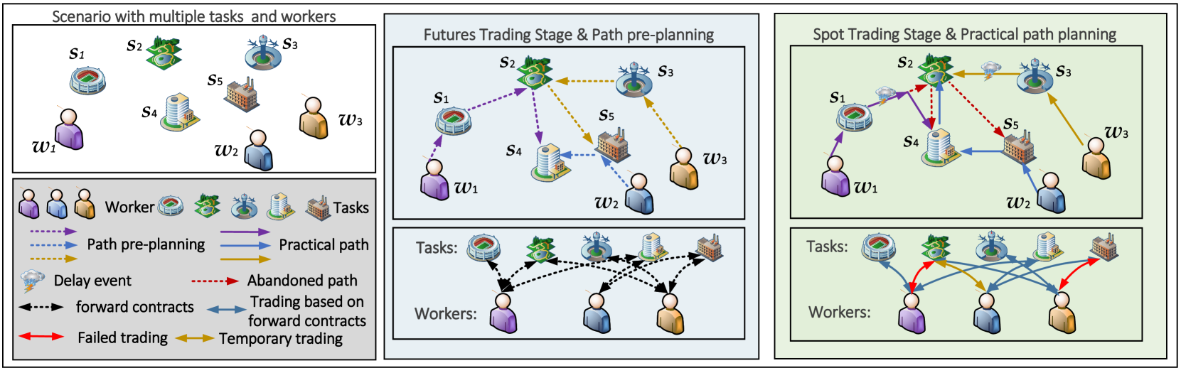
Figure 1: Framework and procedure in terms of a timeline associated with our proposed the stagewise trading framework in dynamic MCS networks.

We are interested in a dynamic MCS network involving two key parties: i) multiple sensing tasks collected in set $\bm{S}=\left\{s_{1},...,s_{i},...,s_{|\bm{S}|}\right\}$, and ii) multiple workers gathered via set $\bm{W}=\left\{w_{1},...,w_{j},...,w_{|\bm{W}|}\right\}$. To capture the time-varying features, a practical transaction is discretized into $T$ timeslots, with index $t$, i.e., $t\in\left\{0,1,2,...,T\right\}$. Also, to describe the dynamic and random nature of real-world MCS networks, we also involve the following uncertain factors:

$\bullet$ Uncertain delay event: Worker $w_{j}$ may encounter delay events (e.g., traffic jam, traffic accident) on the way to task $s_{i}$. We denote the delay event as a random variable $\alpha_{i,j}$, following a Bernoulli distribution $\alpha_{i,j}\sim{\bf B}\left\{(1,0),(a_{i,j},1-a_{i,j})\right\}$. Specifically, $\alpha_{i,j}=1$ indicates that the $w_{j}$ encounters a delay event on its way to $s_{i}$, while $\alpha_{i,j}=0$, otherwise.

$\bullet$ Uncertain duration of the delay event: When encountering a delay event, worker $w_{j}$ will definitely spend a certain amount of time on it, which, to simplify our analysis, can be quantized by the number of timeslots denoted by $\tau^{\text{delay}}$. This duration follows a discrete uniform distribution, denoted by $\tau^{\text{delay}}\sim\mathbf{U}(t^{\text{min}},t^{\text{max}})$, e.g., $\tau^{\text{delay}}\in\{t^{\text{min}},t^{\text{min}}+1,...,t^{\text{max}}-1,t^{\text{max}}\}$.

$\bullet$ Time-varying channel quality: The network condition between a worker and a task owner is denoted by $\gamma_{i,j}$, reflected by the channel quality of wireless link between $w_{j}$ and the nearby access point (AP) for accessing $s_{i}$. The $\gamma_{i,j}$ follows a uniform distribution $\gamma_{i,j}\sim{\bf U}(\mu_{1},\mu_{2})$, where fluctuations can due to factors such as mobility of workers, and obstacles.

In this paper, we explore a novel matching-based stagewise service trading paradigm over dynamic MCS networks with the above uncertain factors. Interestingly, “stagewise” allows us to divide the whole trading process across multiple timeslots as two complementary stages. The former stage relies on a futures trading mode, which encourages each task to recruit a set of workers with paid services, e.g., the corresponding payment (denoted by $p_{i,j}$). While each worker can serve a vector of tasks, where the matched tasks are sorted into a path (sequence) by following factors such as the tasks’ locations, time windows, payments, and costs. In addition, compensation from $w_{j}$ to $s_{i}$ (denoted by $q_{i,j}$) may also be incurred when $w_{j}$ fails to complete $s_{i}$, e.g., $w_{j}$ encounters a set of delay events on the way to $s_{i}$, resulting in insufficient time in performing tasks. The above process can be implemented by facilitating mutually beneficial long-term contracts between workers and tasks, which are pre-signed (e.g., contract terms including $p_{i,j}$ and $q_{i,j}$) in advance to future practical transactions according to historical statistics. With these contracts in place, contractual workers and tasks can engage in practical transactions directly. As a complement, the latter stage relies on a spot trading mode, in which workers and tasks with long-term contracts are expected to fulfill their obligations accordingly. Since workers may fail to complete contractual tasks due to dynamic nature of MCS networks, tasks can further employ temporary workers when experiencing unsatisfying service quality.

Fig. 1 depicts a schematic of the stagewise service trading market. For instance, workers and tasks first sign proper long-term contracts with pre-planned paths (the intermediate two boxes of Fig. 1). During a practical transaction (the right two boxes of Fig. 1), worker $s_{1}$ gives up $s_{2}$ to proceed to the next task. Similarly, worker $s_{3}$ decides to continue $s_{2}$, but fails to complete $s_{5}$. Also, due to uncertain factors, long-term workers may not be able to catch the deadline of assigned tasks. During this time, task owners with remaining budgets can recruit temporary workers (e.g., in Fig. 1, $s_{2}$ recruits $w_{2}$).

3.2 Basic Modeling

Modeling of Tasks: The attribute of each MCS task $s_{i}\in\bm{S}$ is represented by a 6-tuple $\langle t_{i}^{\text{b}},t_{i}^{\text{e}},B_{i},Q_{i}^{\text{D}},l_{i}^{\text{s}},d_{i}\rangle$, where $t_{i}^{\text{b}}$ and $t_{i}^{\text{e}}$ define the start and closing time of $s_{i}$ (in terms of timeslot, e.g., $s_{i}$ starts at the $t_{i}^{\text{b}}$-th timeslot), collectively form a time window. Additionally, $B_{i}$ denotes the budget of task $s_{i}$, constraining the number of employable workers; $Q_{i}^{\text{D}}$ represents the desired service quality of $s_{i}$ (e.g., its required AoI); the location of $s_{i}$ is given by $l_{i}^{\text{s}}=(lo_{i}^{\text{s}},la_{i}^{\text{s}})$, where $lo_{i}^{\text{s}}$ and $la_{i}^{\text{s}}$ represent the longitude and latitude of $s_{i}$, respectively. The data size that each worker provides to $s_{i}$ is denoted by $d_{i}$ (e.g., bits).

Modeling of Workers: The attribute of a worker $w_{j}\in\bm{W}$ is described by a 6-tuple $\langle e_{j}^{\text{c}},e_{j}^{\text{D}},e_{j}^{\text{t}},e_{j}^{\text{m}},f_{j},v_{j},l_{j}^{\text{w}}\langle t\rangle\rangle$, where $e_{j}^{\text{c}}$ (e.g., dollar/timeslot), $e_{j}^{\text{D}}$ (e.g., dollar/timeslot), $e_{j}^{\text{t}}$ (e.g., J/timeslot), and $e_{j}^{\text{m}}$ (e.g., dollar/timeslot) indicate the cost consumed in each timeslot for data collection, delay event, data transmission, and traveling to the target task, respectively. Note that for $e_{j}^{\text{c}}$, $e_{j}^{\text{D}}$, and $e_{j}^{\text{m}}$, we consider a monetary representation to better describe a resource trading market. Besides, $f_{j}$ (e.g., bits) represents the size of data collected by worker $w_{j}$ in each timeslot, and the moving speed of worker $w_{j}$ is denoted by $v_{j}$ (e.g., meter/timeslot). The position of $w_{j}$ at timeslot $t$ is represented by $l_{j}^{\text{w}}\langle t\rangle=(lo_{j}^{\text{w}}\langle t\rangle,la_{j}^{\text{w}}\langle t\rangle)$, where $lo_{j}^{\text{w}}\langle t\rangle$ and $la_{j}^{\text{w}}\langle t\rangle$ denote the longitude and latitude of worker $w_{j}$, respectively.

4 Proposed FT-SMP³

4.1 Key Modeling

We first define the matching between tasks and workers:

$\bullet$ $\varphi(s_{i})$: the set of workers recruited for processing task $s_{i}$, i.e., $\varphi(s_{i})\in\bm{W}$;

$\bullet$ $\varphi(w_{j})$: the vector of sensing tasks assigned to worker $w_{j}$, i.e., $\varphi(w_{j})\in\bm{S}$;

Notably, we replace notations $p_{i,j}$, $q_{i,j}$ during futures trading stage by $p^{F}_{i,j}$, $q^{F}_{i,j}$, to avoid possible confusion with spot trading stage.

4.1.1 Utility, expected utility, and risk of workers

As performing tasks can incur costs on workers, we consider four types of costs for worker $w_{j}$ to complete task $s_{i}$:

i) Moving cost. The Euclidean distance between task $s_{i}$ and worker $w_{j}$ at timeslot $t$ is calculated as $Ed_{i,j}\langle t\rangle=\left((lo_{j}^{\text{w}}\langle t\rangle-lo_{i}^{\text{s}})^{2}+(la_{j}^{\text{w}}\langle t\rangle-la_{i}^{\text{s}})^{2}\right)^{\frac{1}{2}}$. Besides, we can have the time for $w_{j}$ moving to $s_{i}$ as $\tau_{i,j}^{\text{move}}\langle t\rangle=\frac{Ed_{i,j}\langle t\rangle}{v_{j}}$. Accordingly, the moving cost at timeslot $t$ can be expressed by

$$c_{i,j}^{\text{move}}\langle t\rangle=e_{j}^{\text{m}}\tau_{i,j}^{\text{move}}\langle t\rangle=\frac{e_{j}^{\text{m}}Ed_{i,j}\langle t\rangle}{v_{j}}.$$ (1)

ii) Sensing cost. The time that worker $w_{j}$ spends on collecting data for task $s_{i}$ is defined as $\tau_{i,j}^{\text{sense}}=\frac{d_{i}}{f_{j}}$. Thus, we calculate the data collection cost as

$$c_{i,j}^{\text{sense}}=e_{j}^{\text{c}}\tau_{i,j}^{\text{sense}}=\frac{e_{j}^{\text{c}}d_{i}}{f_{j}}.$$ (2)

iii) Transmission cost. The time consumed by worker $w_{j}$ transmitting sensing data to $s_{i}$ as

$$\tau_{i,j}^{\text{tran}}=\frac{d_{i}}{W\text{log}_{2}\left(1+e_{j}^{\text{t}}\gamma_{i,j}\right)},$$ (3)

where $W$ is the bandwidth of wireless communication links, and $e_{j}^{\text{t}}\gamma_{i,j}$ indicates the received signal noise ratio (SNR) of $s_{i}$. The transmission cost is expressed by

$$c_{i,j}^{\text{tran}}=e_{j}^{\text{t}}\tau_{i,j}^{\text{tran}}=\frac{\mathbb{V}_{1}e_{j}^{\text{t}}d_{i}}{W\text{log}_{2}\left(1+e_{j}^{\text{t}}\gamma_{i,j}\right)},$$ (4)

where $\mathbb{V}_{1}$ is the unit monetary cost/Joule (e.g., dollar/J).

iv) Cost incurred by delay event. Since a worker $w_{j}$ may encounter delay events to task $s_{i}$, we define the delay time for worker $w_{j}$ traveling to $s_{i}$ as $\tau_{i,j}^{\text{D}}\langle t^{\text{ini}}\rangle=\sum_{n=1}^{\tau_{i,j}^{\text{move}}\langle t^{\text{ini}}\rangle}\alpha_{i,j}\tau^{\text{delay}}_{n}$, where $t_{i,j}^{\text{ini}}$ represents the initial timeslot for $w_{j}$ to set off for task $s_{i}\in\varphi(w_{j})$. The cost incurred by a delay event can thus be calculated as

$$c_{i,j}^{\text{D}}\langle t^{\text{ini}}\rangle=e_{j}^{\text{D}}\tau_{i,j}^{\text{D}}\langle t^{\text{ini}}\rangle.$$ (5)

Accordingly, the overall cost on $w_{j}$ performing $s_{i}$ is

$$c_{i,j}\langle t^{\text{ini}}\rangle=c_{i,j}^{\text{move}}\langle t^{\text{ini}}\rangle+c_{i,j}^{\text{D}}+c_{i,j}^{\text{sense}}+c_{i,j}^{\text{tran}},$$ (6)

and the corresponding task completion time is given by

$$\tau_{i,j}\langle t^{\text{ini}}\rangle=\tau_{i,j}^{\text{move}}\langle t^{\text{ini}}\rangle+\tau_{i,j}^{\text{D}}\langle t^{\text{ini}}\rangle+\tau_{i,j}^{\text{sense}}+\tau_{i,j}^{\text{tran}}.$$ (7)

Since worker $w_{j}$ may encounter delay events and accordingly fails to complete a task in time, we use $\beta_{i,j}$ to describe whether $w_{j}$ completes $s_{i}$ during practical transactions, as given by

$$\beta_{i,j}=\left\{\begin{aligned} &0,~~w_{j}\text{ breaks a contract with }s_{i}\\ &1,~~w_{j}\text{ fulfills a contract with }s_{i}.\end{aligned}\right.$$ (8)

The utility of worker $w_{j}$ involves three key components: i) the overall payment minus the cost on performing tasks, ii) the service cost which has been consumed on $w_{j}$, while confronting a failure in task completion, and iii) the penalty for failing to complete tasks. Accordingly, the utility of worker $w_{j}$ is given by

$$U^{W}(w_{j},\varphi(w_{j}))=\sum_{s_{i}\in\varphi(w_{j})}\beta_{i,j}\left(p^{F}_{i,j}-c_{i,j}\langle t_{i,j}^{\text{ini}}\rangle\right)$$ (9)

$$-\sum_{s_{i}\in\varphi(w_{j})}(1-\beta_{i,j})\left(c_{i,j}^{\text{part}}\langle t_{i,j}^{\text{ini}}\rangle+q^{F}_{i,j}\right),$$

where $c_{i,j}^{\text{part}}\langle t_{i,j}^{\text{ini}}\rangle$ indicates the costs incurred when worker $w_{j}$ has made efforts but task $s_{i}$ still fails. This cost structure is similar to that of $c_{i,j}\langle t_{i,j}^{\text{ini}}\rangle$, including movement costs, delay event costs, sensing costs, and transmission costs. The specific value of $c_{i,j}^{\text{part}}\langle t_{i,j}^{\text{ini}}\rangle$ is determined by the timeslot in which worker $w_{j}$ decides to abandon task $s_{i}$. Apparently, uncertain factors can impose challenges to obtain the practical value of (9) in our designed futures trading stage. Instead, we are interested in its expection, as shown below

$$\overline{U^{W}}(w_{j},\varphi(w_{j}))=\text{E}[{U^{W}}(w_{j},\varphi(w_{j}))]$$ (10)

$$= \sum_{s_{i}\in\varphi(w_{j})}\text{E}[\beta_{i,j}]\left(p^{F}_{i,j}-\text{E}[c_{i,j}\langle t_{i,j}^{\text{ini}}\rangle]\right)-$$

$$\sum_{s_{i}\in\varphi(w_{j})}\left(1-\text{E}[\beta_{i,j}]\right)\left(\text{E}[c_{i,j}^{\text{part}}\langle t_{i,j}^{\text{ini}}\rangle]+q^{F}_{i,j}\right),$$

where derivations of $\text{E}\left[\beta_{i,j}\right]$, $\text{E}\left[c_{i,j}\langle t_{i,j}^{\text{ini}}\rangle\right]$, and $\text{E}\left[c_{i,j}^{\text{part}}\langle t_{i,j}^{\text{ini}}\rangle\right]$ are detailed in Appx. B.1.

A futures trading can generally bring both benefits and risks, as uncertainties may lead to losses to participants. Thus, we evaluate two specific risks for each worker:

i) The risk of receiving an unsatisfying utility: Each worker $w_{j}\in\bm{W}$ serving task $s_{i}\in\varphi(w_{j})$ faces the risk of obtaining an unsatisfying utility (e.g., when the value of $U^{W}(w_{j},s_{i})$ turns negative) during a practical transaction. This risk is defined by the probability that the utility $U^{W}(w_{j},s_{i})$ falls below a tolerable value $u_{\text{min}}$, given by:

$$R^{W}_{1}(w_{j},s_{i})=\text{Pr}\left(U^{W}(w_{j},s_{i})<u_{\text{min}}\right),~\forall s_{i}\in\varphi(w_{j}),$$ (11)

where $u_{\text{min}}$ is a positive value approaching to 0.

ii) The risk on failing to complete the task: The time for a worker $w_{j}$ to complete task $s_{i}\in\varphi(w_{j})$ may be insufficient due to possible delay events, as defined by

$$R_{2}^{W}(w_{j},s_{i})=\text{Pr}\left(\beta_{i,j}=0\right),~~~\forall s_{i}\in\varphi(w_{j}).$$ (12)

The aforementioned risks should be managed within an acceptable range, otherwise, worker $w_{j}$ will not sign a long-term contract with task $s_{i}$ during the futures trading stage.

4.1.2 Utility, expected utility, and risk of tasks

Considering the importance of freshness of MCS data, we use age of information (AoI) as a crucial assessment service quality. In particular, the life cycle of data generally begins when data are collected/sensed, and ends when they are delivered to the task owner. During this process, the AoI raises with time goes by. Inspired by existing literature[7, 21], let $t_{i,j}^{\text{gen}}$ denote the timeslot when worker $w_{j}$ starts collecting data for task $s_{i}$ (each timeslot generates data of size $f_{j}$, e.g., bits/timeslot). Then, the AoI of sensing data that $w_{j}$ provides to $s_{i}$ can be defined as

$$age_{i,j}=f_{j}\sum_{t^{\prime}=t_{i,j}^{\text{gen}}+\tau_{i,j}^{\text{tran}}}^{t_{i,j}^{\text{gen}}+\tau_{i,j}^{\text{sense}}+\tau_{i,j}^{\text{tran}}}\left(t^{\prime}-t_{i,j}^{\text{gen}}\right).$$ (13)

Accordingly, the average AoI of overall sensing data that $w_{j}$ contributes to $s_{i}$ can be calculated as $AGE_{i,j}=\frac{age_{i,j}}{d_{i}}$. Thus, let $Q\left(s_{i},\varphi(s_{i})\right)$ describe the service quality that task $s_{i}$ receives from the worker set $\varphi(s_{i})$, as given by

$$Q\left(s_{i},\varphi(s_{i})\right)=\sum_{w_{j}\in\varphi(s_{i})}\frac{1}{AGE_{i,j}}~.$$ (14)

Accordingly, the utility of task $s_{i}$ consists of two key parts: i) the obtained service quality; ii) the remaining budget (a larger remaining budget further reflects a lower cost), as given by

$$U^{S}(s_{i},\varphi(s_{i}))=\mathbb{V}_{2}\sum_{w_{j}\in\varphi(s_{i})}\frac{1}{AGE_{i,j}}+$$ (15)

$$\mathbb{V}_{3}\left(\sum_{w_{j}\in\varphi(s_{i})}\left((1-\beta_{i,j})q^{F}_{i,j}-\beta_{i,j}p^{F}_{i,j}\right)\right),$$

where $\mathbb{V}_{2}$ and $\mathbb{V}_{3}$ are positive weighting coefficients. As uncertainties prevent us from getting the practical value of the task’s utility directly, we consider its corresponding expectation as

$$\overline{U^{S}}\left(s_{i},\varphi(s_{i})\right)=\text{E}[U^{S}\left(s_{i},\varphi(s_{i})\right)]$$ (16)

$$= \mathbb{V}_{2}\frac{1}{\text{E}[AGE_{i,j}]}+$$

$$\mathbb{V}_{3}\left(\sum_{w_{j}\in\varphi(s_{i})}\left((1-\text{E}[\beta_{i,j}])q^{F}_{i,j}-\text{E}[\beta_{i,j}]p^{F}_{i,j}\right)\right),$$

where derivations of $\text{E}[AGE_{i,j}]$ is detailed in Appx. B.2.

Similar to workers, task owners also face risks owing to market dynamics. This risk of $s_{i}$ is primarily associated with the inability to reach desired service quality, given by

$$R^{S}(s_{i},\varphi(s_{i}))=\text{Pr}\left(Q(s_{i},\varphi(s_{i}))<Q_{i}^{\text{D}}\right).$$ (17)

Apparently, a larger value of $R^{S}(s_{i},\varphi(s_{i}))$ implies a higher risk on an unsatisfying quality. Thus, the task owner will not sign long-term contracts with workers in the futures trading stage when confronting an unacceptable risk.

4.2 Key Definitions of Matching

We next introduce our designed matching in futures trading stage, representing an unique many-to-many (M2M) matching tailored to the characteristics of uncertainties, upon considering multiple timeslots. More importantly, this matching is also crafted to cope with potential risks in dynamic MCS networks, distinguishing it from conventional matching mechanisms.

Definition 1.

(M2M matching of FT-SMP³) A M2M matching $\varphi$ of our proposed FT-SMP³ constitutes a mapping between task set $\bm{S}$ and worker set $\bm{W}$, which satisfies the following properties:

$\bullet$ for each task $s_{i}\in\bm{S},\varphi\left(s_{i}\right)\subseteq\bm{W}$,

$\bullet$ for each worker $w_{j}\in\bm{W},\varphi\left(w_{j}\right)\subseteq\bm{S}$,

$\bullet$ for each task $s_{i}$ and worker $w_{j}$, $s_{i}\in\varphi(w_{j})$ if and only if $w_{j}\in\varphi\left(s_{i}\right)$.

We next define the blocking coalition, which is a crucial factor that can make the matching unstable.

Definition 2.

(Blocking coalition) Under a given matching $\varphi$, worker $w_{j}$ and task vector $\mathbb{S}\subseteq\bm{S}$ may form one of the following two types of blocking coalition, denoted by $\left(w_{j};\mathbb{S}\right)$.

Type 1 blocking coalition: Type 1 blocking coalition satisfies the following two conditions:

$\bullet$ Worker $w_{j}$ prefers a task vector $\mathbb{S}\subseteq\bm{S}$ rather than its currently matched task vector $\varphi(w_{j})$, i.e.,

$$\overline{U^{W}}(w_{j},\mathbb{S})>\overline{U^{W}}(w_{j},\varphi(w_{j})).$$ (18)

$\bullet$ Every task in $\mathbb{S}$ prefers to recruit workers rather than being matched to its currently matched/assigned worker set. That is, for any task $s_{i}\in\mathbb{S}$, there exists a worker set $\varphi^{\prime}(s_{i})$ that constitutes the workers that need to be evicted, satisfying

$$\overline{U^{S}}\left(s_{i},\left\{\varphi\left(s_{i}\right)\backslash\varphi^{\prime}\left(s_{i}\right)\right\}\cup\left\{w_{j}\right\}\right)>\overline{U^{S}}\left(s_{i},\varphi\left(s_{i}\right)\right).$$ (19)

Type 2 blocking coalition: Type 2 blocking coalition satisfies the following two conditions:

$\bullet$ Worker $w_{j}$ prefers executing task vector $\mathbb{S}\subseteq\bm{S}$ to its currently matched task vector $\varphi(w_{j})$, i.e.,

$$\overline{U^{W}}(w_{j},\mathbb{S})>\overline{U^{W}}(w_{j},\varphi(w_{j})).$$ (20)

$\bullet$ Every task in $\mathbb{S}$ prefers to further recruit worker $w_{j}$ in conjunction to its currently matched/assigned worker set. That is, for any task $s_{i}\in\mathbb{S}$, we have

$$\overline{U^{S}}(s_{i},\varphi(s_{i})\cup\left\{w_{j}\right\})>\overline{U^{S}}(s_{i},\varphi(s_{i})).$$ (21)

Recall the above definitions, the Type 1 blocking coalition can lead to the unstability of matching since a task is incentivized to recruit another set of workers that can bring it with a higher expected utility. Similarly, the Type 2 blocking coalition makes the matching unstable since the task has a left-over budget to recruit more workers, which can further helps with increasing its expected utility.

4.3 Problem Formulation

We conduct the service provisioning in futures trading stage as a M2M matching, occurring prior to practical transactions. Our goal is to achieve stable mappings between tasks and workers to facilitate long-term contracts. Accordingly, each task $s_{i}\in\bm{S}$ aims to maximize its overall expected utility, which is mathematically formulated as the following optimization problem:

$$\bm{\mathcal{F}^{S}}:~ \underset{{\varphi\left(s_{i}\right)}}{\max}~\overline{U^{S}}\left(s_{i},\varphi\left(s_{i}\right)\right)$$ (22)

s.t. $$\varphi\left(s_{i}\right)\subseteq\bm{W}$$ (22a)

$$\sum_{w_{j}\in\varphi(s_{i})}p^{F}_{i,j}\leq B_{i}$$ (22b)

$$R^{S}_{1}\left(s_{i},\varphi\left(s_{i}\right)\right)\leq\rho_{1},$$ (22c)

where $0<\rho_{1}\leq 1$ represents a risk threshold. In $\bm{\mathcal{F}^{S}}$, constraint (22a) forces the recruited workers $\varphi(s_{i})$ within set $\bm{W}$, constraint (22b) ensures that the expenses of task $s_{i}$ devoted to recruiting workers $\varphi(s_{i})$ does not exceed its budget $B_{i}$, and constraint (22c) dictates the tolerance of each task on receiving an undesired utility, with its derivation detailed in Appx. B.2. Furthermore, each worker $w_{j}\in\bm{W}$ aims to maximize its expected utility, as modeled by

$$\bm{\mathcal{F}^{W}}:~ \underset{{\varphi\left(w_{j}\right)}}{\max}~\overline{U^{W}}\left(w_{j},\varphi\left(w_{j}\right)\right)$$ (23)

s.t. $$\varphi\left(w_{j}\right)\subseteq\bm{S}$$ (23a)

$$c_{i,j}\leq p^{F}_{i,j},~\forall s_{i}\in\varphi\left(w_{j}\right)$$ (23b)

$$R^{W}_{1}\left(w_{j},s_{i}\right)\leq\rho_{2},~\forall s_{i}\in\varphi\left(w_{j}\right)$$ (23c)

$$R^{W}_{2}\left(w_{j},s_{i}\right)\leq\rho_{3},~\forall s_{i}\in\varphi\left(w_{j}\right),$$ (23d)

where $\rho_{2}$ and $\rho_{3}$ are risk thresholds falling in interval $(0,1]$. In $\bm{\mathcal{F}^{W}}$, constraint (23a) ensures that task set $\varphi(w_{j})$ belongs to set $\bm{S}$, and constraint (23b) shows that the payments asked by $w_{j}$ can cover the corresponding service costs; constraints (23c) and (23d) manages the possible risks that each worker may confront during practical transactions, with their derivation detailed in Appx. B.1.

Our proposed futures trading stage aims to solve a multi-objective optimization (MOO) problem that involves (22) and (23). Conventional M2M matching are typically based on determined market to achieve stable matching. However, when confronted with dynamic MCS networks and potential risks, conventional M2M matching approaches cannot directly address these challenges. After extensive investigations, we delve into a combination of an improved heuristic method and a futures-based M2M stable matching algorithms to tackle the MOO problem, detailed by the following section.

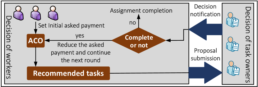
Figure 2: A flow chart, showing the distributed task-worker interaction model regarding our proposed FT-SMP³.

4.4 Solution Design

$$pr^{\mathbbm{k}}_{m,n}=\left\{\begin{aligned} &\frac{\tau^{\varepsilon_{1}}_{m,n}\eta^{\varepsilon_{2}}_{m,n}(1/width_{n})^{\varepsilon_{3}}(1/wait_{n})^{\varepsilon_{4}}}{\sum_{k\in J_{\mathbbm{k}}(m)}\tau^{\varepsilon_{1}}_{m,n}\eta^{\varepsilon_{2}}_{m,n}(1/width_{n})^{\varepsilon_{3}}(1/wait_{n})^{\varepsilon_{4}}},~~~\text{if }n\in J_{\mathbbm{k}}(m)\\ &0,~~~~~~~~~~~~~~~~~~~~~~~~~~~~~~~~~~~~~~~~~~~~~~~~~~~~~~~~~~~~~~~~~~~~~~~~~~\text{otherwise}\end{aligned}\right.$$ (24)

We next develop the futures trading-driven stable matching and pre-path-planning (FT-SMP³) to achieve efficient and stable matching between workers and time-dependent tasks, thereby obtaining i) a set of long-term contracts among them to guide future transactions, and ii) the path that each worker may follow. Specifically, FT-SMP³ consists of two key algorithms: i) enhanced ant colony optimization for path pre-planning and task recommendation (EACO-P³TR), taking into account diverse task demands, payments that workers can receive, and costs for performing tasks, which aims to recommend tasks to workers along with corresponding pre-planned paths; and ii) futures trading-driven many-to-many (FT-M2M) matching, enabling long-term contracts between workers and tasks to achieve stable services.

Fig. 2 shows the flow chart of our proposed FT-SMP³, where the interaction between task owners and workers can be realized through deploying multiple rounds. Key steps are detailed below:

$\bullet$ At the beginning of each round, each worker determines its interested tasks through our proposed EACO-P³TR algorithm, to obtain its maximum expected utility. The worker then announces its information to its interested tasks.

$\bullet$ After collecting workers’ reports, each task temporarily selects some workers who can offer the highest expected service quality as candidates, under its budget constraints (i.e., (22b)), and then informs all the workers.

$\bullet$ Following the decisions of tasks, if a worker is rejected by a task, it can reduce its asked payments to enhance its competitiveness in the next round; while if it is selected, its asked payment remains unchanged in the next round.

$\bullet$ Repeat the above steps until either of the following conditions are met: i) all workers are recruited by their interested tasks; ii) no worker can further reduce its asked payments (e.g., to avoid negative utility and controlling risks).

4.4.1 Proposed EACO-P³TR Algorithm

Inspired by the ant colony optimization (ACO)[22] algorithm upon considering diverse characteristics of tasks (e.g., varying time windows and locations) and workers (e.g., various costs), we develop the EACO-P³TR algorithm. This algorithm recommends proper tasks to each worker along with a pre-planned path (e.g., the sequence of tasks), to maximize workers’ expected utility. Regarding a worker $w_{j}$ and all the tasks as vertices and the edges between them, we construct a directed complete graph denoted by $\bm{G_{j}}(\bm{V_{j}},\bm{E_{j}})$. In this graph, $\bm{V_{j}}=\left\{v_{0},v_{1},\ldots,v_{|\bm{S}|}\right\}$ represents the set of vertices ($v_{0}$ denotes the worker $w_{j}$, $v_{1},...,v_{|\bm{S}|}$ represent tasks), indexed by $m$ and $n$ for convenience of analysis, and $\bm{E_{j}}=\left\{(v_{m},v_{n})|v_{m},v_{n}\in\bm{V_{j}},m\neq n\right\}$ comprises the edge set. Note that the location of $v_{0}$ is denoted by $l^{\text{w}}_{j}\langle 0\rangle$, and the locations of $v_{1},v_{2},\ldots,v_{|\bm{S}|}$ are $l^{\text{s}}_{1},l^{\text{s}}_{2},\ldots,l^{\text{s}}_{|\bm{S}|}$.

In EACO-P³TR, we use a set $\bm{\mathbb{K}}$ to denote the collection of ants. Each ant $\mathbbm{k}\in\mathbb{K}$ simulates the moving trajectory of worker $w_{j}$, namely, starting from $v_{0}$. It considers comprehensive information such as the current timeslot, the time window of tasks, the location of vertices, the expected timeslot required to travel to each task, and the expected utility upon reaching each task, while then selects a feasible vertice to visit next (i.e., the current timeslot adds the expected travel time from the current position to the target vertice is early the end of the target vertice’s time window). This process continues until no visitable applicable vertices left. The state transition rule of EACO-P³TR, i.e., the probability of ant $\mathbbm{k}$ moving from task $v_{m}$ to $v_{n}$ ($m\neq n\neq 0$), can be defined as (24), where $\varepsilon_{1}$, $\varepsilon_{2}$, $\varepsilon_{3}$, and $\varepsilon_{4}$ are positive weight coefficients. Besides, $\tau_{m,n}$ represents the pheromone deposited for the transition from $v_{m}$ to $v_{n}$, as given by (25), while $\eta_{m,n}$ denotes the distance between $v_{m}$ and $v_{n}$, and $width_{n}$ denotes the width of the time window for task $s_{i}$ in vertice $v_{n}$ (i.e., $width_{n}=t_{i}^{\text{e}}-t_{i}^{\text{b}}$). Moreover, $wait_{n}$ represents the waiting time if the ant arrives early (e.g., before the task starts), where $wait_{n}=\max\left\{t_{n}^{\text{b}}-(t_{m,n}^{\text{ini}}+\tau_{m,n}^{\text{move}}+\tau_{m,n}^{\text{D}}),0\right\}$. Moreover, $J_{\mathbbm{k}}(m)$ is the set of remaining feasible tasks that ant $\mathbbm{k}$ can complete at vertice $v_{m}$, and the tasks $s_{i}\in J_{\mathbbm{k}}(m)$ should satisfy constraints (23c) and (23d).

When a path has been found by the ant colony, pheromones along with the edges are updated as

$$\tau_{m,n}\leftarrow(1-\theta)\tau_{m,n}+\mathrm{\Delta}\tau_{m,n},$$ (25)

where $0<\theta<1$ is the pheromone evaporation coefficient, and $\mathrm{\Delta}\tau_{m,n}$ is the pheromone deposited by ants, which can be calculated as

$$\mathrm{\Delta}\tau_{m,n}=\left\{\begin{aligned} &\sum_{(v_{m},v_{n})\in\bm{M^{\text{max}}}}\triangle\overline{U^{W}_{m,n}},~\text{if edge }(v_{m},v_{n})\in\bm{M^{\text{max}}}\\ &0,~~~~~~~~~~~~~~~~~~~~~~~~~~~~~~~~~~\text{otherwise},\end{aligned}\right.$$ (26)

where $\triangle\overline{U^{W}_{m,n}}$ denotes the expected utility for worker $w_{j}$ from vertice $v_{m}$ to finish the task in vertice $v_{n}$. $\bm{M^{\text{max}}}$ is the path (e.g., a vector of the completed tasks of $w_{j}$) with the maximum utility obtained from all ants, i.e., $\bm{M^{\text{max}}}=\left\{\bm{M^{\mathbbm{k}}}|\max~\sum_{(m,n)\in\bm{M^{\mathbbm{k}}}}\triangle\overline{U^{W}_{m,n}},~\forall\mathbbm{k}\in\mathbb{K}\right\}$.

1 Input: worker $w_{j}$, task set $\bm{S}$ 

2Initialization: $\tau_{m,n}\leftarrow\tau_{0}$, $iter=1$, $v_{m}=v_{0}$, $iter_{\text{max}}$, $\mathbb{K}$

3while $iter\leq iter_{\text{max}}$ do

4    for $\forall k\in\mathbb{K}$ do

5       $\bm{M^{\mathbbm{k}}}=\varnothing$

6      while not end condition do

7         Calculate: $J_{\mathbbm{k}}(m)$, $pr^{\mathbbm{k}}_{m,n}$

8         if $\forall J_{\mathbbm{k}}(m)\neq\varnothing$ then

9            $n\leftarrow$ ant $\mathbbm{k}$ randomly selects the next task $n$ from $J_{\mathbbm{k}}(m)$ according to $pr^{\mathbbm{k}}_{m,n}$

10            $\bm{M^{\mathbbm{k}}}\leftarrow\left\{\text{edge}(m,n)\right\}\cup\bm{M^{\mathbbm{k}}}$

11            $m\leftarrow n$

12         else

13            break loop

14         

15      

16   

17   $\bm{M^{\text{max}}}\leftarrow\left\{\bm{M^{\mathbbm{k}}}|\max~\sum_{(m,n)\in\bm{M^{\mathbbm{k}}}}\triangle\overline{U^{W}_{m,n}},~\forall k\in\bm{K}\right\}$

18   update $\tau_{m,n}$

19   $iter=iter+1$

20$L^{\text{best}}_{j}\leftarrow$ selects the task vector from $\bm{M^{\text{max}}}$

Output: $L^{\text{best}}_{j}$

Algorithm 1 Proposed EACO-P³TR Algorithm

Alg. 1 details the pseudo-code of our designed EACO-P³TR algorithm, including several key steps:

Step 1. Initialization: According to the information associated with workers and tasks (e.g., their locations, time windows of tasks, payments of workers, and the expected time and energy consumed on performing tasks), Alg. 1 starts with constructing a directed complete graph $\bm{G_{j}}(\bm{V_{j}},\bm{E_{j}})$ for each worker $w_{j}$, denoted by $v_{0}$.

Step 2. Path exploration: In each iteration, ant $\mathbbm{k}$ at each vertice evaluates multiple factors involving: the present time, the expected time traveling to the next unvisited vertice, the expected time to perform the task, and the time window. This evaluation is conducted to ascertain whether the task can be completed within the specified time frame, thereby obtaining $J_{\mathbbm{k}}(m)$ and $pr^{\mathbbm{k}}_{m,n}$ (line 7, Alg. 1). Then, the next vertice (task) is chosen from set $J_{\mathbbm{k}}(m)$ according to (24). This iteration proceeds until no further executable vertices (line 8, Alg. 1).

Step 3. Pheromone update: Subsequently, the expected utilities $\sum_{(m,n)\in\bm{M^{\mathbbm{k}}}}\triangle\overline{U^{W}_{m,n}}$ associated with different vertice sequence $\bm{M^{\mathbbm{k}}}$ are compared, among which, the path with the maximum expected utility (i.e., $\bm{M^{\text{max}}}$) is selected for pheromone updating (lines 14-15, Alg. 1), following the procedures outlined in (25) and (26).

Step 4. Optimal path output: After finishing all the iterations, the route $\bm{M^{\text{max}}}$ with the highest expected utility can be determined as the pre-planned path for worker $w_{j}$. Accordingly, the tasks along this path are recommended.

4.4.2 Proposed FT-M2M matching algorithm

1 Initialization: $k\leftarrow 1$, $p_{i,j}\left\langle 1\right\rangle\leftarrow p^{\text{Desire}}_{i,j}$, for $\forall i,j$, ${flag}_{j}\leftarrow 1$, $\mathbb{Y}\left(w_{j}\right)\leftarrow\varnothing$, $\mathbb{Y}\left(s_{i}\right)\leftarrow\varnothing$ 

2while ${flag}_{j}$ do

3    ${flag}_{j}\leftarrow 0$

4   $L^{\text{best}}_{j}\leftarrow\text{Alg. 1}$, $\mathbb{Y}\left(w_{j}\right)\leftarrow L^{\text{best}}_{j}$

5   if $\forall\mathbb{Y}\left(w_{j}\right)\neq\varnothing$ then

6       for $\forall s_{i}\in\mathbb{Y}\left(w_{j}\right)$ do

7         $w_{j}$ sends a proposal about its information to $s_{i}$

8      

9      while  $\Sigma_{w_{j}\in\bm{W}}{flag}_{j}>0$ do

10          Collect proposals from the workers in $\bm{W}$, e.g., using ${\widetilde{\mathbb{Y}}}\left(s_{i}\right)$ to include the workers that send proposals to $s_{i}$

11         $\mathbb{Y}(s_{i})\leftarrow$ choose workers from ${\widetilde{\mathbb{Y}}}\left(s_{i}\right)$ that can achieve the maximization of the expected utility by using DP under budget $B_{i}$

12         $s_{i}$ temporally accepts the workers in $\mathbb{Y}(s_{i})$, and rejects the others

13      

14      for  $\forall s_{i}\in\mathbb{Y}\left(w_{j}\right)$  do

15          if $w_{j}$ is rejected by $s_{i}$, $p_{i,j}\left\langle k\right\rangle>c_{i,j}$, and risk constraint (23c) is met then

16             $p_{i,j}\left\langle{k+1}\right\rangle\leftarrow\max\left\{p_{i,j}\left\langle k\right\rangle-\mathrm{\Delta}p~,{c}_{i,j}\right\}$

17         else

18            $p_{i,j}\left\langle{k+1}\right\rangle\leftarrow p_{i,j}\left\langle k\right\rangle$

19         

20      

21      if there exists $p_{i,j}\left\langle{k+1}\right\rangle\neq p_{i,j}\left\langle k\right\rangle\$, $\forall s_{i}\in\mathbb{Y}\left(w_{j}\right)$ then

22          ${flag}_{j}\leftarrow 1$, $k\leftarrow k+1$ 

23      

24   

25

26if  $R^{S}\left(s_{i},\varphi\left(s_{i}\right)\right)\leq\rho_{1}$ then

27   $s_{i}$ gives up trading in the futures trading stage

28

29$\varphi(s_{i})\leftarrow\mathbb{Y}(s_{i})$, $\varphi(w_{j})\leftarrow\mathbb{Y}(w_{j})$

Return: $\varphi(s_{i})$, $\varphi(w_{j})$, $L_{j}^{\text{best}}$.

Algorithm 2 Proposed FT-M2M Matching Algorithm

Following the pre-planned paths, we then introduce FT-M2M matching (see Alg. 2), which facilitates stable, efficient, and risk-aware matching between tasks and workers, as well as their long-term contracts.

Step 1. Initialization: At the beginning of Alg. 2, each worker $w_{j}$’s asked payment is set by $p_{i,j}\left\langle 1\right\rangle=p^{\text{Desire}}_{i,j}$ (line 1, Alg. 2), $\mathbb{Y}(w_{j})$ contains the interested tasks of $w_{j}$ and $\mathbb{Y}(s_{i})$ involves the workers temporarily selected by $s_{i}$.

Step 2. Proposal of workers: At each round $k$, each worker $w_{j}$ first chooses tasks from $L^{\text{best}}_{j}$ (the optimal task vector for worker $w_{j}$ according to its expected utility, derived from Alg. 1), and records them in $\mathbb{Y}(w_{j})$. Then, $w_{j}$ sends a proposal to each task in $\mathbb{Y}(w_{j})$, including its asked payments $p_{i,j}\left\langle k\right\rangle$, probability of completing $s_{i}$ (i.e., $\beta_{i,j}$), and expected service quality of sensing data $\text{E}[Q_{i,j}]$ (line 7, Alg. 2).

Step 3. Worker selection on tasks’ side: After collecting the information from workers in set ${\widetilde{\mathbb{Y}}}\left(s_{i}\right)$, each task $s_{i}$ solves a 0-1 knapsack problem, which can generally be solved via dynamic programming (DP) [8, 23, 24] (line 10, Alg. 2), determine a collection of temporary workers (e.g., set $\mathbb{Y}(s_{i})$), where $\mathbb{Y}(s_{i})\subseteq{\widetilde{\mathbb{Y}}}\left(s_{i}\right)$ that can bring the maximum expected utility, under budget $B_{i}$. Then, each $s_{i}$ reports its decision on worker selection during the current round to workers.

Step 4. Decision-making on workers’ side: After obtaining the decisions from each task $s_{i}\in\mathbb{Y}(w_{j})$, worker $w_{j}$ inspects the following conditions:

$\bullet$ Condition 1. If $w_{j}$ is accepted by $s_{i}$ or its current asked payment $p_{i,j}\left\langle k\right\rangle$ equals to its cost ${\ c}_{i,j}$ or risk constraint (23c) isn’t met, its payment remains unchanged (line 16, Alg. 2);

$\bullet$ Condition 2. If $w_{j}$ is rejected by a task $s_{i}$, its asked payment $p_{i,j}\left\langle k\right\rangle$ can still cover its cost ${c}_{i,j}$ and risk constraint (23c) is met, it decreases its asked payment for $s_{i}$ in the next round, while avoiding a negative utility (line 14, Alg. 2):

$$p_{i,j}\left\langle{k+1}\right\rangle=\max\left\{p_{i,j}\left\langle k\right\rangle-\mathrm{\Delta}p_{j}~,{~c}_{i,j}\right\}.$$ (27)

Step 5. Repeat: If all the asked payments stay unchanged from $(k-1)^{\text{th}}$ round to $k^{\text{th}}$ round, the matching terminates at round $k$. We use $\Sigma_{w_{j}\in\bm{W}}{flag}_{j}=0$ to denote this situation (line 3, Alg. 2). Otherwise, the algorithm repeats the above steps (e.g., lines 2-18, Alg. 2) in the next round.

Step 6. Risk analysis: When the algorithm is terminated, each task $s_{i}$ will choose whether to sign long-term contracts with the matched workers according to its risk estimation (constraint (22c)).

4.5 Crucial Design Properties

As our FT-M2M matching algorithm is deployed before future practical transactions, our focus lies in distinctive objectives, e.g., the expectation of workers’ and tasks’ utilities, as well as control of potential risk, which greatly differs from conventional matching mechanisms. Hereafter, we will cover key properties on designing our unique matching in futures trading stage.

Definition 3.

(Individual rationality of FT-M2M matching) For both tasks and workers, a matching $\varphi$ is individually rational when the following conditions are satisfied:

$\bullet$ For tasks: i) the overall payment of a task $s_{i}$ paid to matched workers $\varphi\left(s_{i}\right)$ does not exceed $B_{i}$, i.e., constraint (22b) is met; ii) the risk of each task receiving an undesired service quality is controlled within a certain range, i.e., constraint (22c) is satisfied.

$\bullet$ For workers: i) the risk of each worker receiving an undesired expected utility is controlled within a certain range, i.e., constraint (23c) is satisfied; ii) the risk of each worker failing to complete matched tasks is controlled within a certain range, i.e., constraint (23d) is satisfied.

Definition 4.

(Fairness of FT-M2M matching): A matching $\varphi$ is fair if and only if it does not impose type 1 blocking coalition.

Definition 5.

(Non-wastefulness of FT-M2M matching): A matching $\varphi$ is non-wasteful if and only if it does not impose type 2 blocking coalition.

Definition 6.

(Strong stability of FT-M2M matching) The proposed matching is strongly stable if it is individual rational, fair, and non-wasteful.

Note that competitive equilibrium represents a conventional concept in economic behaviors, playing an important role in analyzing the performance of commodity markets upon having flexible prices and multiple players. When the considered market arrives at the competitive equilibrium, there exists a price at which the number of task owners that will pay is equal to the number of workers that will sell[25]. Correspondingly, the competitive equilibrium of FT-M2M matching is defined below.

Definition 7.

(Competitive equilibrium associated with trading between workers and task owners in futures trading stage) The trading between workers and task owners reaches a competitive equilibrium if the following conditions are satisfied:

$\bullet$ For each worker $w_{j}\in\bm{W}$, if $w_{j}$ is associated with a task owner $s_{i}\in\bm{S}$, then $\text{E}[c_{i,j}]\leq p^{F}_{i,j}$,

$\bullet$ For each task $s_{i}\in\bm{S}$, $s_{i}$ is willing to trade with the worker that can bring it with the maximum expected utility,

$\bullet$ For each task $s_{i}$ in set $\bm{S}$, when $s_{i}$ does not recruit more workers, it indicates that the remaining budget after deducting the payments made to matched workers is insufficient to recruit an additional worker.

For a multi-objective optimization problem (e.g., $\bm{\mathcal{F}^{W}}$ and $\bm{\mathcal{F}^{S}}$), a Pareto improvement occurs when the expected social welfare (referring to a summation of expected utilities of workers and task owners in our considered market) can be increased with another feasible matching result[25]. Thus, a matching is weak Pareto optimal when there is no Pareto improvement.

Definition 8.

(Weak Pareto optimality of trading between tasks and workers in futures trading stage) The proposed matching is weak Pareto optimal if there is no Pareto improvement.

We show that our proposed FT-M2M matching of FT-SMP³ can support the above-discussed properties, while the corresponding analysis and proofs are given by Appx. C, due to space limitation.

5 Proposed ST-DP²WR Mechanism

Workers and tasks with long-term contracts can fulfill the pre-determined contracts and paths directly during a practical transaction, thanks to our well-designed futures trading. Nevertheless, due to the dynamic and uncertain characteristics of MCS networks (e.g., possible delay events), workers may not always reliably complete tasks on the pre-planed path. To address this, we propose the spot trading-driven DQN path planning and onsite worker recruitment (ST-DP²WR) mechanism as a quick and reliable backup, to ensure the utilities for both workers and tasks, including i) for workers, we investigate a deep q-network with prioritized experience replay-enhanced dynamic route optimization (DQNP-DRO) algorithm. This algorithm assists workers to decide whether to follow the pre-planned path, to abandon a contractual task (e.g., a worker can not get to a task in time due to delay events), or to select a new task (which has not been listed in the pre-planned path). And ii) for tasks with unsatisfying service quality (some workers may be unable to serve them due to uncertain delay events), we introduce the spot trading-based temporal many-to-many (ST-M2M) matching algorithm, helping them recruit temporary workers during each practical transaction. To avoid confusion with futures trading, we rewrite $p_{i,j}$, $q_{i,j}$, and $\beta_{i,j}$ in the spot trading stage as $p^{S}_{i,j}$, $q^{S}_{i,j}$, and $\beta_{i,j}^{S}$, respectively.

To facilitate analysis, we define several key notations:

$\bullet$ $\bm{W^{\prime}}\langle t\rangle$: the set of workers that can serve temporary tasks at timeslot $t$, i.e., $\bm{W^{\prime}}\langle t\rangle\in\bm{W}$;

$\bullet$ $\bm{S^{\prime}}\langle t\rangle$: the set of sensing tasks that have surplus budget to recruit temporary workers at timeslot $t$;

$\bullet$ $\nu_{t}(s_{i})$: the set of workers temporary recruited for processing task $s_{i}$ at timeslot $t$, i.e., $\nu_{t}(s_{i})\in\bm{W^{\prime}}\langle t\rangle$;

$\bullet$ $\nu_{t}(w_{j})$: the set of sensing tasks temporary assigned to worker $w_{j}$ at timeslot $t$, i.e., $\nu_{t}(w_{j})\in\bm{S^{\prime}}\langle t\rangle$.

5.1 Utility of tasks and workers

Utility of task $s_{i}\in\bm{S^{\prime}}\langle t\rangle$ consists of two parts: i) obtained service quality, and ii) remaining budget, as given by

$$U^{S\prime}_{t}(s_{i},\nu_{t}(s_{i}))=\mathbb{V}_{2}\sum_{w_{j}\in\nu_{t}(s_{i})}\frac{1}{AGE_{i,j}}+$$ (28)

$$\mathbb{V}_{3}\left(-\sum_{w_{j}\in\nu_{t}(s_{i})}\left((1-\beta_{i,j}^{S})q_{i,j}^{S}-\beta_{i,j}^{S}p_{i,j}^{S}\right)\right).$$

We also define the utility of worker $w_{j}\in\bm{W^{\prime}}$ to encompass three key parts: i) the overall payment minus the cost of completing tasks, ii) the service cost for failing to complete tasks, and iii) the penalty incurred by worker $w_{j}$ for failing to complete tasks. This is given by:

$$U_{t}^{W\prime}(w_{j},\nu_{t}(w_{j}))=\sum_{s_{i}\in\nu_{t}(w_{j})}\beta_{i,j}^{S}\left(p_{i,j}^{S}-c_{i,j}\langle t_{i,j}^{\text{ini}}\rangle\right)$$ (29)

$$-\sum_{s_{i}\in\nu_{t}(w_{j})}(1-\beta_{i,j}^{S})\left(c_{i,j}^{\text{part}}\langle t_{i,j}^{\text{ini}}\rangle+q_{i,j}^{S}\right).$$

Due to the dynamic nature of the MCS networks, workers during this stage can still confront risks:

i) The risk of receiving an unsatisfying utility: Each worker $w_{j}\in\bm{W}$ serving task $s_{i}\in\nu_{t}(w_{j})$ faces the risk of obtaining an unsatisfying utility, given by:

$$R^{W\prime}_{1}(w_{j},s_{i})=\text{Pr}\left(U^{W\prime}_{t}(w_{j},s_{i})<u_{\text{min}}\right),~\forall s_{i}\in\nu_{t}(w_{j})$$ (30)

ii) The risk on failing to complete the task: Each worker $w_{j}$ may not have enough time to complete task $s_{i}\in\nu_{t}(w_{j})$ due to delay events, as defined by

$$R_{2}^{W\prime}(w_{j},s_{i})=\text{Pr}\left(\beta_{i,j}^{S}=0\right),~~~\forall s_{i}\in\nu_{t}(w_{j}).$$ (31)

Besides, the aforementioned risks should be managed within an acceptable range; otherwise, worker $w_{j}$ will not service task $s_{i}$.

5.2 Problem Formulation

In the spot trading stage, each task $s_{i}\in\bm{S^{\prime}}\langle t\rangle$ aims to maximize its overall utility, which can be mathematically formulated as the following optimization problem:

$$\bm{\mathcal{F}^{S\prime}}:~ \underset{{\nu_{t}\left(s_{i}\right)}}{\max}~U_{t}^{S\prime}\left(s_{i},\nu_{t}\left(s_{i}\right)\right)$$ (32)

s.t. $$\nu_{t}\left(s_{i}\right)\subseteq\bm{W^{\prime}}\langle t\rangle$$ (32a)

$$\sum_{w_{j}\in\nu_{t}(s_{i})}p^{s}_{i,j}\leq B_{i}^{t},$$ (32b)

where $B_{i}^{t}$ represents the available budget of task $s_{i}$ at timeslot $t$, also includes the compensation from workers for can not complete $s_{i}$ prior to timeslot $t$ (as stipulated in long-term contracts). In $\bm{\mathcal{F}^{S\prime}}$, constraint (32a) forces recruited workers $\nu_{t}(s_{i})$ to belong to set $\bm{W^{\prime}}\langle t\rangle$, constraint (32b) ensures that the expense of task $s_{i}$ devoted to recruiting workers $\nu_{t}(s_{i})$ does not exceed the its remaining budget $B_{i}^{t}$. Besides, each worker $w_{j}\in\bm{W^{\prime}}$ aims to maximize its utility, as follow

$$\bm{\mathcal{F}^{W\prime}}:~ \underset{{\nu_{t}\left(w_{j}\right)}}{\max}~{U_{t}^{W\prime}}\left(w_{j},\nu_{t}\left(w_{j}\right)\right)$$ (33)

s.t. $$\nu_{t}\left(w_{j}\right)\subseteq\bm{S^{\prime}}\langle t\rangle$$ (33a)

$$c_{i,j}\langle t^{\text{ini}}\rangle\leq p^{s}_{i,j},~\forall s_{i}\in\nu_{t}\left(w_{j}\right)$$ (33b)

$$R^{W^{\prime}}_{1}\left(w_{j},s_{i}\right)\leq\rho_{4},~\forall s_{i}\in\nu_{t}\left(w_{j}\right)$$ (33c)

$$R^{W^{\prime}}_{2}\left(w_{j},s_{i}\right)\leq\rho_{5},~\forall s_{i}\in\nu_{t}\left(w_{j}\right),$$ (33d)

where $\rho_{4}$ and $\rho_{5}$ are risk thresholds fall in interval $(0,1]$. In $\bm{\mathcal{F}^{W\prime}}$, constraint (33a) ensures that task set $\nu_{t}(w_{j})$ belongs to set $\bm{S^{\prime}}\langle t\rangle$, and constraint (33b) ensures the payments asked by $w_{j}$ can cover their service costs; constraints (33c) and (33d) control possible risks, and their derivations are detailed by Appx. D.

The ST-M2M matching algorithm focuses on a MOO problem. Our goal is to achieve stable and efficient matching between tasks that require temporary recruitment and workers during a specific timeslot in spot trading stage, thereby enhancing the service quality obtained by the tasks through temporary recruitment.

5.3 Solution Design

Facing dynamic networks and uncertainties factors (e.g., delay events), workers need to make decisions through our proposed DQNP-DRO algorithm (i.e., whether to abandon the current task or continue with it) to maximize their utility. For tasks that are abandoned, recruiting temporary workers through ST-M2M matching can be a good option to enhance task completion rates and improve their utility. Hereafter, we will introduce our proposed DQNP-DRO algorithm.

Our studied problem represents as a Markov Decision Process (MDP), for which Deep Q-Network (DQN)[27] offers an useful technique that integrates Q-learning with deep neural networks, as benefiting from its online learning and the function approximation capabilities. Accordingly, our proposed DQNP-DRO algorithm implements on a DQN model with prioritized experience replay (PER)[26].

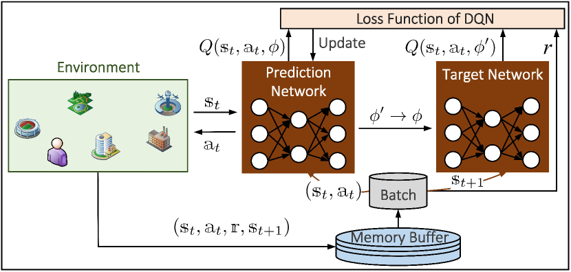
Figure 3: A detailed structure of the ST-DP²WR.

Fig. 3 depicts the schematic of our proposed DQNP-DRO algorithm, where our considered dynamic MCS network is conceptualized as an environment with multiple agents. Meanwhile, each worker is seen as a DQN agent, making decisions on the observed state of the environment whether to continue the current task or choose next task following vector $\varphi(w_{j})$. The goal of the agent is to discover an optimal policy $\pi$, maximizing long-term cumulative rewards by taking an action $\mathbbm{a}$ under a given state $\mathbbm{s}$. Optimal state-action values can be found through the Q-function based on state-action pairs, defined as

$$Q(\mathbbm{s}_{t},\mathbbm{a}_{t})={\bf E}_{\pi}\left[\sum_{i=1}^{\infty}\chi^{i-1}\mathbb{R}_{t+i}|\mathbb{S}_{t}=\mathbbm{s},\mathbb{A}_{t}=\mathbbm{a}\right],$$ (34)

where $\chi$ is a discount factor ($0\leq\chi\leq 1$), and $\mathbb{R}_{t}$ is a reward that the agent can obtain by taking action $\mathbbm{a}_{t}$ in state $\mathbbm{s}_{t}$. Q-learning uses a Q-table to store Q-values and the online updating rule of the Q-values with a learning rate $lr$ ($0\leq lr\leq 1$) is given by

$$Q(\mathbbm{s}_{t},\mathbbm{a}_{t})\leftarrow$$ (35)

$$Q(\mathbbm{s}_{t},\mathbbm{a}_{t})+lr\left[\mathbbm{r}_{t}+\chi\underset{{\mathbbm{a}}}{\max}Q(\mathbbm{s}_{t+1},\mathbbm{a}_{t})-Q(\mathbbm{s}_{t},\mathbbm{a}_{t})\right].$$

The state, action and reward function for the proposed DQNP-DRO algorithm are defined as follows:

$\bullet$ State: the state is composed of five elements: i) worker’s current location; ii) current timeslot; iii) target task; iv) information required for executing the task (e.g., the sequence of tasks, locations and time windows of tasks, and penalties for abandoning tasks); and v) the distance from the worker to the current target task.

$\bullet$ Action: the action considers two main factors: i) continue with the selected task, and ii) abandon the current task and choose the next task following the pre-path $L_{j}^{\text{best}}$.

$\bullet$ Reward: the reward function accounts for four conditions: i) if the worker is on its way to the task and chooses to continue, a negative reward is given for moving loss (e.g., $c_{i,j}^{\text{move}}$); ii) if the worker plans to change the current task, a negative reward can be caused for contract break (e.g., $q_{i,j}^{F}$ or $q_{i,j}^{S}$); iii) upon reaching the task, a negative reward is incurred for the cost of data collection and transmission (e.g., $c_{i,j}^{\text{sense}}+c_{i,j}^{\text{tran}}$); and iv) completing the task yields a positive reward (e.g., $p_{i,j}^{F}$ or $p_{i,j}^{S}$).

Unlike Q-learning, DQN uses a deep neural network to approximate the optimal state-action value Q-function, i.e., $Q(\mathbbm{s},\mathbbm{a},\theta^{\prime})\approx\underset{\pi}{\max}~Q(\mathbbm{s},\mathbbm{a})$, where $\theta^{\prime}$ denotes a set of parameters for a neural network. The training process of the DQN includes the following steps:

$\bullet$ Initialize the memory buffer size, structure and parameters of the DQN.

$\bullet$ Interact with the environment and generate a set of training data. Each interaction generates a tuple $(\mathbbm{s}_{t},\mathbbm{a}_{t},\mathbbm{r}_{t},\mathbbm{s}_{t+1})$.

$\bullet$ Store the experience-tuples into the memory buffer.

$\bullet$ By employing a strategy of PER[26], a batch of experience tuples of specified size is sampled from the memory buffer. These data are then input into the DQN, where the value of the loss function can be calculated by (36)

$$Loss=\left[\mathbbm{r}_{t}+\chi\underset{\mathbbm{a}}{\max}Q(\mathbbm{s}_{t+1},\mathbbm{a}_{t+1},\phi^{\prime})-Q(\mathbbm{s}_{t},\mathbbm{a}_{t},\phi^{\prime})\right]^{2},$$ (36)

where $\phi$ and $\phi^{\prime}$ are parameters of a prediction network and those of a target network in the DQN, respectively. $Q(\mathbbm{s}_{t},\mathbbm{a}_{t},\phi^{\prime})$ is the output of the prediction network, while $\underset{\mathbbm{a}}{\max}~Q(\mathbbm{s}_{t+1},\mathbbm{a}_{t+1},\phi^{\prime})$ represents the output of the target network.

$\bullet$ Use an RMSprop method[28] to update the parameters of DQN until the values of the loss function converge.

$\bullet$ Replace the parameters of the target network by that of the prediction network after a certain number of training steps.

1

2Initialization: $t=0$, $\bm{S^{\prime}}\langle t\rangle\leftarrow\varnothing$, $L_{j}$, DQN-PER network of worker $w_{j}$

3for episode = 1, 2, 3, …  do

4    for $t=1,2,...,\bm{T}$ do

5       if $\bm{S^{\prime}_{t}}\neq\varnothing$ then

6          $\nu_{t}(w_{j})\leftarrow$ ST2M matching algorithm

7      for $\forall w_{j}\in\bm{W}$ do

8         

9         $L_{j}\leftarrow L_{j}\cup\nu_{t}(w_{j})$

10         Observe state $\mathbbm{s}_{t}$

11         Select action $\mathbbm{a}_{t}$ using $\varepsilon$-greedy strategy

12         if $w_{j}$ choose to give up task $s_{i}\in\varphi\left(w_{j}\right)$ then

13            $\bm{S^{\prime}}\langle t\rangle\leftarrow\bm{S^{\prime}}\langle t\rangle\cup\left\{s_{i}\right\}$

14         

15         Get reward $\mathbbm{r}_{t}$ and the next state $\mathbbm{s}_{t+1})$

16         Store $(\mathbbm{s}_{t},\mathbbm{a}_{t},\mathbbm{r}_{t},\mathbbm{s}_{t+1})$ into the memory buffer

17         Update the DQN-PER network of worker $w_{j}$

18      if $\forall w_{j}\in\bm{W}$ complete all accepted tasks that can be completed then

19          Break

20      

21   Continue till all reward of workers convergence

22

Algorithm 3 Proposed DQNP-DRO Algorithm

We next detail our proposed DQNP-DRO algorithm (given by Alg. 3).

Step 1. Initialization: We first initialize the relevant parameters, where timeslot $t=0$, the set of tasks requiring temporary recruitment $\bm{S^{\prime}}\langle t\rangle$ is empty set, and initialize the DQN-PER network for each worker $w_{j}\in\bm{W}$.

Step 2. Temporary task-worker determination: When there are tasks with unsatisfying service quality (line 4, Alg. 3), we study a ST-M2M matching algorithm to match workers with tasks, while outputting the corresponding task set $\nu_{t}(w_{j})$. Subsequently, the worker adds these tasks in $\nu_{t}(w_{j})$ to $L_{j}$ (line 7, Alg. 3). Since ST-M2M matching works under a similar way to FT-M2M matching in some aspects, its details (e.g., algorithm design, key properties and corresponding proofs) are moved to Appx. E.

Step 3. DQN model training: Before taking an action, worker $w_{j}$ first observes the current state of the environment. Based on which, it takes action through the DQN, obtain the corresponding reward, and update the state to $\mathbbm{s}_{t+1}$ (lines 8 to 9, Alg. 3). Next, information related to timeslot $t+1$ is stored in the memory buffer, and the DQN is updated using the PER strategy. This process is repeated continuously until no more tasks can be completed (lines 3 to 16, Alg. 3).

Step 4. Repetition: Steps 1 to 3 are repeatedly performed until the reward converges (line 17, Alg. 3).

6 Evaluation

We conduct comprehensive evaluations to verify the effectiveness of our methodology, which are carried out via Python 3.9 with 13th Gen Intel Core i9-13900K*32 and NVIDIA GeForce RTX 4080. Recall the previous sections, our proposed FT-SMP³ and ST-DP²WR work together to facilitate a stagewise trading paradigm, which are collectively abbreviated as “StagewiseTM³atch” in this section, for analytical simplicity.

6.1 Simulation Settings

To better emulate a dynamic MCS network, we utilize the real-world dataset of Chicago taxi trips[29] that records taxi rides in Chicago from 2013 to 2016 with 77 community areas. Our simulations consider the 77-th community area as our sensing region [24], with 271259 data points.

To capture the inherent randomness of tasks, they are randomly distributed within the considered region. Moreover, to better quantify the service costs of workers, we focus on specific information from the dataset, including using the pick-up locations of taxis as the initial positions of workers (e.g., $l^{\text{w}}_{j}\langle 0\rangle$), the average speed of taxis (i.e., travel distance/travel time) to estimate the speed of workers moving towards a task (e.g., $v_{j}$), and the taxi fare to quantify the energy cost of workers during traveling (e.g., $e^{m}_{j}$). Accordingly, key parameters are set as [24, 13, 11, 30, 31]: $\bm{T}=100$, $\alpha_{i,j}\in[0.005,0.01]$, $\tau_{i,j}^{\text{D}}\in[1,5]$ timeslots, $\mu_{1}=150$, $\mu_{2}=400$ (i.e., the received SNR thus falls within $[17,23]$ dB roughly), $t_{i}^{\text{b}}\in[1,90]$, $t_{i}^{\text{e}}\in[10+t_{i}^{\text{b}},99+t_{i}^{\text{b}}]~(\text{note that }t_{i}^{\text{e}}\leq\bm{T})$, $B_{i}\in[30,45]$, $Q_{i}^{\text{D}}\in[20,35]$, $d_{i}\in[2,4]$ Gb, $e_{j}^{\text{c}}\in[0.002,0.006]$ $/timeslot, $e_{j}^{\text{t}}\in[450,550]$ mW, $e_{j}^{\text{m}}\in[0.02,0.05]$ $/timeslot, $f_{j}\in[256,512]$ Mb/timeslot, $v_{j}\in[100,200]$ m/timeslot, $W=6$ MHz, thresholds $\rho_{1},...,\rho_{5}=0.3$, $\bm{K}=20$.

Moreover, for definiteness and without loss of generality, we are inspired by the Monte Carlo method and conduct 100 simulations for each figure in this section.

6.2 Benchmark Methods and Evaluation Metrics

To conduct better evaluations, we involve comparable benchmark methods from diverse perspectives. Regarding the conventional spot trading mode, we consider spot trading-enabled M2M matching (ConSpotTM³atch), which borrows the idea from [17], mapping each worker to a vector of tasks by analyzing the current network conditions. To underscore the significance on meeting diverse demands of time-dependent tasks, we involve spot trading-enabled M2M matching without considering task demands on location and time window (ConSpotTM³atch\TD), as inspired by [8], which mirrors ConSpotTM³atch but disregards the location and timeliness of tasks. To emphasize the importance of risk control in dynamic networks, we introduce a benchmark called stagewise trading-enabled M2M matching without risk analysis (StagewiseTM³atch\Risk), which is analogous to our StagewiseTM³atch but excludes risk analysis (i.e., constraints (22c), (23c), (23d), (33c), and (33d)). To explore the trade-off between time efficiency and resource allocation performance, we introduce another two benchmarks under spot trading mode: service quality-preferred method (Quality_P) and random matching (Random_M), borrowing the ideas from [32], where tasks in Quality_P prefer workers with the highest service quality under budget constraints; while Random_M randomly selects workers under budget constraints.

To conduct quantitative evaluations, we also focus on crucial performance metrics detailed in the following:

$\bullet$ Service quality: As one of the most important factors in MCS networks, service quality is calculated by the overall received service quality of tasks.

$\bullet$ Utility of tasks and workers: The utilities received by tasks and workers.

$\bullet$ Social welfare: The summation of utilities of both tasks and workers.

$\bullet$ The proportion of tasks that meet their desired service quality (PoDSQ): PoDSQ represents the ratio of tasks that meet their desired service quality to the overall tasks.

$\bullet$ The proportion of tasks abandoned by workers (PoTAW): PoTAW represents the ratio of tasks abandoned by workers to the overall tasks accepted by workers.

$\bullet$ Running time (RT, ms): The running time is obtained by Python on verison 3.9, reflecting time efficiency.

$\bullet$ Number of interactions (NI): Total number of interactions between tasks (owners) and workers to obtain matching decisions, reflecting the overhead on decision-making.

6.3 Performance Evaluations

6.3.1 Service quality, utility, and social welfare

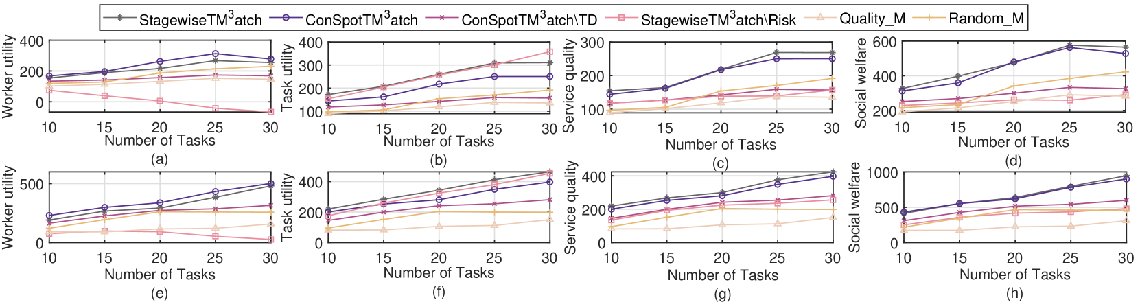
Figure 4: Performance comparisons in terms of utility of workers, utility of tasks, service quality and social welfare under different problem sizes, where (a)-(d) consider 15 workers, and (e)-(h) consider 30 workers in the network.

We study the performance of our proposed StagewiseTM³atch method in terms of utility of workers and tasks, service quality and social welfare, in Fig. 4. To capture various problem scales, Figs. 4(a)-4(d) consider 15 workers, while Figs. 4(e)-4(h) consider 30 workers.

Fig. 4(a) illustrates that our proposed StagewiseTM³atch method achieves the highest service quality, thanks to the stagewise mode that comprehensively considers task diversity and risks in dynamic networks. In contrast, ConSpotTM³atch performs slightly worse, because it only employs spot trading mode. Furthermore, our StagewiseTM³atch significantly outperforms the other four benchmark methods, due to the drawbacks in their fundamental matching logic. For instance, ConSpotTM³atch\TD neglects the diversity of task requirements, StagewiseTM³atch\Risk overlooks risk management, and Quality_P focuses solely on task utility, thus significantly increasing the probability of failures in performing tasks. Additionally, due to the inherent randomness of Random_M, it faces unsatisfactory service quality of tasks. Note that in Fig. 4(a), the curves of StagewiseTM³atch and ConSpotTM³atch slightly decline after 25 tasks, since the time window limits the number of tasks that workers can complete. The performance shown in Fig. 4(e) is similar to that of Fig. 4(a). However, after 25 tasks, Fig. 4(e) features more workers and can serve more tasks compared to Fig. 4(a). Therefore, as the number of tasks increases, the curves for StagewiseTM³atch and ConSpotTM³atch in Fig. 4(e) continue to rise.

We next show Fig. 4(b) and Fig. 4(f) to evaluate the performance on tasks’ utility, consisting of received service quality and the remaining financial budget (further reflects the costs for purchasing services). Methods such as ConSpotTM³atch, ConSpotTM³atch\TD, Quality_P, and Random_M do not incorporate compensations for tasks, thus enabling performance similar to that in Fig. 4(a) and Fig. 4(e). In contrast, StagewiseTM³atch compensates those tasks with default workers, thereby allowing more budget to recruit temporary workers. Notably, StagewiseTM³atch\Risk overlooks risk analysis for either workers or tasks, leading to a high incidence of trading failures. As for workers, Fig. 4(c) and Fig. 4(g) reveal that ConSpotTM³atch achieves the best performance on their utilities, which attributed to the consideration of task diversity and risk management, striving to complete more matched tasks successfully. Our StagewiseTM³atch achieves slightly lower workers’ utility than that of ConSpotTM³atch, since workers in our consideration may have to make compensations to tasks. Besides, StagewiseTM³atch\Risk method accepts a high number of tasks without analyzing risks. Thus, more service failures can be incurred with the rising number of tasks, e.g., workers have to pay to those tasks they can not complete, due to factors such as delay events. Other benchmark methods, either failing to adequately consider task diversity or employing simplistic matching strategies, result in a significant reduction in the number of tasks completed by workers, thus affecting the utility of the workers.

In Fig. 4(d) and Fig. 4(h), our StagewiseTM³atch depicts the best performance on social welfare, further demonstrating that we can handle diverse demands of tasks and thanks to risk management. Such performance can highlight our superiority in balancing the social welfare optimization across various market scales.

6.3.2 PoDSQ and PoTAW

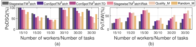
Figure 5: Performance comparisons in terms of PoDSQ and PoTAW.

As the uncertain factors can prevent workers from completing assigned tasks, further leading to trading failures and unsatisfying service quality, we involve PoDSQ and PoTAW as two crucial significant factors, upon having various problem scales (see Fig. 5).

As shown in Fig. 5(a), our method StagewiseTM³atch outperforms other methods on FoSDQ, as attributed to the well-designed stagewise mechanism, as well as the effective risk analysis, allowing our proposed method to surpass the service quality of the existing advanced ConSpotTM³atch. In contrast, since ConSpotTM³atch\TD and StagewiseTM³atch\Risk overlook diverse task demands and risk controls, the values of FoSDQ of them stay lower. Furthermore, the inherent factor on greediness and randomness of Quality_P and Random_M bring them with less satisfactory outcomes, further reflecting poor trading experience of task owners.

Since this paper considers real-world factors in MCS networks, e.g., an uncertain delay event and its duration, workers may be unable to catch the deadline of every task, thus forcing them to give up some assigned tasks. To evaluate the task abandon rate, which reflects the trading experience for both workers and task owners in the considered MCS networks, we conduct Fig. 5(b). In this figure, we can clearly see that our proposed StagewiseTM³atch consistently outperforms other methods on PoTAW across various problem scales, maintaining a rate below 30%. This impressive performance benefits by our consideration on risk management, to ensure that all matched tasks are controllable and achievable with an acceptable probability. ConSpotTM³atch performs a lower PoTAW than ours due its unilateral concern on a single-stage mechanism, lacking the backup for tasks to recruit more workers, when some workers are facing difficulties to catch the assigned tasks on its half-way, and thus decide to give up. Moreover, StagewiseTM³atch\Risk lacks designs on risk control, ConSpotTM³atch\TD overlooks personal demands of tasks while Quality_P and Random_M rely solely on greedy and random strategies for task assignment. These limitations can cause the situations where workers accept a large number of unachievable tasks, thereby leading to poor performance on PoTAW.

6.3.3 RT and NI

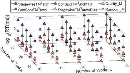
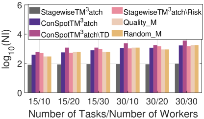
Figure 6: Performance comparisons in terms of RT and NI.

As a primary concern in dynamic networks, efficiency (e.g., time and energy efficiency) represents a significant indicators in evaluating the performance of a service trading market. To demonstrate this, we delve into RT (e.g., time consumed by decision-making) , and NI (e.g., the number of rounds on negotiating factors such as which task/worker to trade with, and trading prices), as illustrated by Fig. 6. For better clarity, logarithmic representation is utilized in this figure to visibly show the gap among different methods.

As observed in Fig. 6(a), ConSpotTM³atch always stays large because it matches tasks to workers during each transaction, based on the current network/market conditions, leading to excessive delay on decision-making. While the RT of our StagewiseTM³atch remains stably lower than ConSpotTM³atch, even having a rising number of tasks and workers. This is because each worker has pre-matched tasks and recommended paths thanks to the pre-signed long-term contracts in futures trading stage, whereas in the spot trading stage, facing the uncertainties of a dynamic networks, workers only need to make minor adjustments. Then, although ConSpotTM³atch\TD and StagewiseTM³atch\Risk outperform ConSpotTM³atch and StagewiseTM³atch in RT, they overlook crucial factors such as the demands of tasks (e.g., time window) and risks, thus leading to unsatisfying performance on utility of workers and tasks, service quality, and social welfare. Furthermore, due to simple ideas adopted by Quality_P and Random_M, these methods exhibit far lower RT as compared to others. However, they exhibit poor performance on service quality (see Figs. 4-5).

Then, Fig. 6(b) describes the performance on NI, which reflects the overhead on decision-making, e.g., energy consumed by workers and task owners for negotiating trading decisions. Apparently, a large value of NI indicates high overhead during the trading process. Fig. 6(b) displays the performance on NI upon having different numbers of tasks and workers, where our StagewiseTM³atch greatly outperforms other methods. Initially, due to that participants in ConSpotTM³atch and ConSpotTM³atch\TD methods have to negotiate a trading decision (e.g., task allocation and service prices) during every practical transaction, undoubtedly increasing time and energy overhead. Specifically, ConSpotTM³atch\TD suffers from the highest NI due to its failure to consider tasks (i.e., location and time window), intensifying competition among workers. Fortunately, StagewiseTM³atch encourages participants to engage in futures trading, thereby enhancing decision-making efficiency. Besides, our proposed StagewiseTM³atch, thanks to well-designed risk management, outperforms StagewiseTM³atch\Risk. Additionally, although Quality_P and Random_M do not focus on bargaining and risk management among participants and only engage in simple interactions (workers notify each task of their willingness, and tasks report their choice on workers), these activities also consume certain overheads, especially when the market scale increases. Our StagewiseTM³atch still outperforms these methods in terms of NI. Note that simulations regarding individual rationality of tasks and workers are moved to Appx. F.

7 Conclusion

We investigate a novel stagewise trading framework that integrates futures and spot trading to facilitate efficient and stable matching between diverse tasks and workers, in a dynamic and uncertain MCS network. In the former stage, we propose FT-SMP³ for long-term task-worker assignment and path pre-planning for workers based on historical statistics and risk analysis. The following stage investigates ST-DP²WR mechanism to enhance workers’ and tasks’ practical utilities by facilitating temporary worker recruitment. Theoretical exploration demonstrates that our proposed mechanisms can support essential properties including individual rationality, strong stability, competitive equilibrium, and weak Pareto optimality. Evaluations through real-world dataset demonstrate our superior performance in comparison to existing methods across various metrics. We are also interested in exploring smart contract design for service trading and potential collaborations among workers, as interesting future directions.

Houyi Qi received his B.S. degree in electronic information engineering from Zhengzhou University, China, in 2021. He is currently working toward the M.S. degree in School of Informatics, Xiamen University, China. His research interests include mobile crowdsensing networks, matching theory and cloud/edge/service computing.

Minghui Liwang (Member, IEEE) is currently an associate professor with the Department of Control Science and Engineering, and the Shanghai Research Institute for Intelligent Autonomous Systems, Tongji University, China. Her research interests include multi-agent systems, edge computing, distributed learning as well as economic models and applications.

Xianbin Wang (Fellow, IEEE) is a Professor and a Tier1 Canada Research Chair in 5G and Wireless IoT Communications with Western University, Canada. His current research interests include 5G/6G technologies, Internet of Things, machine learning, communications security, and intelligent communications. He has over 600 highly cited journals and conference papers, in addition to over 30 granted and pending patents and several standard contributions. Dr. Wang is a Fellow of the Canadian Academy of Engineering and a Fellow of the Engineering Institute of Canada. He has received many prestigious awards and recognitions, including the IEEE Canada R. A. Fessenden Award, Canada Research Chair, Engineering Research Excellence Award at Western University, Canadian Federal Government Public Service Award, Ontario Early Researcher Award, and nine Best Paper Awards. He was involved in many IEEE conferences, including GLOBECOM, ICC, VTC, PIMRC, WCNC, CCECE, and CWIT, in different roles, such as General Chair, TPC Chair, Symposium Chair, Tutorial Instructor, Track Chair, Session Chair, and Keynote Speaker. He serves/has served as the Editor-in-Chief, Associate Editor-in-Chief, and editor/associate editor for over ten journals. He was the Chair of the IEEE ComSoc Signal Processing and Computing for Communications (SPCC) Technical Committee and is currently serving as the Central Area Chair of IEEE Canada.

Liqun Fu (Senior Member, IEEE) is a Full Professor of the School of Informatics at Xiamen University, China. She received her Ph.D. Degree in Information Engineering from The Chinese University of Hong Kong in 2010. She was a post-doctoral research fellow with the Institute of Network Coding of The Chinese University of Hong Kong, and the ACCESS Linnaeus Centre of KTH Royal Institute of Technology during 2011-2013 and 2013-2015, respectively. She was with ShanghaiTech University as an Assistant Professor during 2015-2016. Her research interests are mainly in communication theory, optimization theory, game theory, and learning theory, with applications in wireless networks. She is on the editorial board of IEEE Communications Letters and the Journal of Communications and Information Networks (JCIN). She served as the Technical Program Co-Chair of IEEE/CIC ICCC 2021 and the GCCCN Workshop of the IEEE INFOCOM 2014, the Publicity Co-Chair of the GSNC Workshop of the IEEE INFOCOM 2016, and the Web Chair of the IEEE WiOpt 2018. She also serves as a TPC member for many leading conferences in communications and networking, such as the IEEE INFOCOM, ICC, and GLOBECOM.

Yiguang Hong (Fellow, IEEE) received his B.S. and M.S. degrees from Peking University, China, and the Ph.D. degree from the Chinese Academy of Sciences (CAS), China. He is currently a professor of Shanghai Institute of Intelligent Science and Technology, Tongji University from Oct 2020, and was a professor of Academy of Mathematics and Systems Science, CAS. His current research interests include nonlinear control, multi-agent systems, distributed optimization/game, machine learning, and social networks. Prof. Hong serves as Editor-in-Chief of Control Theory and Technology. He also serves or served as Associate Editors for many journals, including the IEEE Transactions on Automatic Control, IEEE Transactions on Control of Network Systems, and IEEE Control Systems Magazine. He is a recipient of the Guan Zhaozhi Award at the Chinese Control Conference, Young Author Prize of the IFAC World Congress, Young Scientist Award of CAS, the Youth Award for Science and Technology of China, and the National Natural Science Prize of China. He is also a Fellow of IEEE, a Fellow of Chinese Association for Artificial Intelligence, and a Fellow of Chinese Association of Automation (CAA). Additionally, he is the chair of Technical Committee of Control Theory of CAA and was a board of governor of IEEE Control Systems Society.

Li Li (Member, IEEE) is currently a full professor with the Department of Control Science and Engineering, and the Shanghai Research Institute for Intelligent Autonomous Systems, Tongji University, China. She has over 50 publications, including five books, over 30 journal articles, and two book chapters. Her current research interests include data-based modeling and optimization, computational intelligence, and machine learning.

Zhipeng Cheng (Member, IEEE) received his B.S. degree in communication engineering from Jiangnan University, Wuxi, China, in 2017. He received the Ph.D. degree in communication engineering with Xiamen University, Xiamen, China, in 2023. He is now a lecturer in the School of Future Science and Engineering, Soochow University, Suzhou, China. His research interests include UAV communication networks, cloud/edge/service computing, reinforcement learning and distributed machine learning applications.

Appendix A Key Notations

Key notations in this paper are summarized in Table 2.

TABLE II: Key notations

Notation	Explanation
$\bm{S}$, $\bm{W}$, $\bm{S^{\prime}}\langle t\rangle$, $\bm{W^{\prime}}\langle t\rangle$	The MCS sensing task set and worker set in FT-SMP3, ST-DP2WR
$s_{i}$, $w_{j}$	The $i^{\text{th}}$ sensing task in $\bm{S}$, $\bm{S^{\prime}}\langle t\rangle$, the $j^{\text{th}}$ worker in $\bm{W}$, $\bm{W^{\prime}}\langle t\rangle$
$p_{i,j}^{F}$, $p_{i,j}^{S}$	Payment of task $s_{i}$ offered to worker $w_{j}$ in FT-SMP3, ST-DP2WR
$q_{i,j}^{F}$, $q_{i,j}^{S}$	Compensation worker $w_{j}$ offered to task $s_{i}$ in FT-SMP3, ST-DP2WR
$t_{i}^{\text{b}}$, $t_{i}^{\text{e}}$	the start and closing time of $s_{i}$
$Q^{\text{D}}_{i}$	Desired utility for task $s_{i}$
$B_{i}$	Budget for task $s_{i}$
$l_{i}^{\text{s}}$, $l_{j}^{\text{w}}$	Location of task $s_{i}$ and worker $w_{j}$
$d_{i}$	Data size that each worker needs to provide task $s_{i}$
$e_{j}^{\text{c}}$, $e_{j}^{\text{D}}$, $e_{j}^{\text{t}}$, $e_{j}^{\text{m}}$	Cost consumed in each timeslot for data collection, delay event, data transmission, traveling to the target task
$f_{j}$	The size of data collected by worker $w_{j}$ in each timeslot
$v_{j}$	Movement speed of worker $w_{j}$
$\alpha_{i,j}$	Random variable describes encounter delay event of worker $w_{j}$ during moving to task $s_{i}$
$\tau^{\text{delay}}$	Random variable describes uncertain duration of the delay event:
$\gamma_{i,j}$	Random variable describes time-varying channel qualities between worker $w_{j}$ and task $s_{i}$
$c_{i,j}\langle t^{\text{ini}}\rangle$	Service cost of worker $w_{j}$ complete task $s_{i}$
$\tau_{i,j}\langle t^{\text{ini}}\rangle$	The number of timeslots required by worker $w_{j}$ to complete task $s_{i}$.
$\beta_{i,j}$, $\beta^{S}_{i,j}$	Indicator of whether $w_{j}$ will break the contract with $s_{i}$ in FT-SMP3, ST-DP2WR
$\varphi\left(s_{i}\right)$, $\varphi\left(w_{j}\right)$	The set of workers recruited for processing task $s_{i}$ and the set of tasks assigned to worker $w_{j}$ in FT-SMP3
$\nu_{t}\left(s_{i}\right)$, $\nu_{t}\left(w_{j}\right)$	The set of workers recruited for processing task $s_{i}$ and the set of tasks assigned to worker $w_{j}$ in ST-DP2WR
${U^{S}}$, $\overline{U^{S}}$	Utility and expected utility of a task
${U^{W}}$, $\overline{U^{W}}$	Utility and expected utility of a worker
${R^{W}_{1}}$, $R_{2}^{W}$, ${R^{S}}$	Risk associated with workers, tasks in FT-SMP3
${R^{W\prime}_{1}}$, $R_{2}^{W\prime}$	Risk associated with workers in ST-DP2WR

Appendix B Derivations Associated with FT-SMP³

B.1 Derivations related to workers

Mathematical expectation of $c_{i,j}\langle t^{\text{ini}}\rangle$. Random variable $\alpha_{i,j}$ follows a Bernoulli distribution $\alpha_{i,j}\sim{\bf B}\left\{(1,0),(a_{i,j},1-a_{i,j})\right\}$, with its expectation calculated by $\text{E}[\alpha_{i,j}]=1\times a_{i,j}+0\times(1-a_{i,j})=a_{i,j}$. Moreover, $\tau^{\text{delay}}$ obeys an uniform distribution, e.g., $\tau^{\text{delay}}\sim\mathbf{U}(t^{\text{min}},t^{\text{max}})$, while $\text{E}[\tau^{\text{delay}}]$ can accordingly be expressed as $\frac{t^{\text{min}}+t^{\text{max}}}{2}$. Similarly, the expected value of $\gamma_{i,j}$ can be expressed as $\frac{\mu_{1}+\mu_{2}}{2}$. Thus, we have the value of $c_{i,j}\langle t^{\text{ini}}\rangle$ as

$$\text{E}[c_{i,j}\langle t^{\text{ini}}\rangle]= c_{i,j}^{\text{move}}\langle t^{\text{ini}}\rangle+c_{i,j}^{\text{D}}+c_{i,j}^{\text{sense}}+c_{i,j}^{\text{tran}}$$ (37)

$$= c_{i,j}^{\text{move}}\langle t^{\text{ini}}\rangle+c_{i,j}^{\text{sense}}+\text{E}[c_{i,j}^{\text{D}}]+\text{E}[c_{i,j}^{\text{tran}}]$$

$$= c_{i,j}^{\text{move}}\langle t^{\text{ini}}\rangle+c_{i,j}^{\text{sense}}+\frac{\mathbb{V}_{1}e_{j}^{\text{t}}d_{i}}{W\text{log}_{2}\left(1+e_{j}^{\text{t}}\text{E}[\gamma_{i,j}]\right)}+$$

$$\sum_{n=1}^{\tau_{i,j}^{\text{move}}\langle t^{\text{ini}}\rangle}\text{E}[\alpha_{i,j}]\text{E}[\tau^{\text{delay}}_{n}]$$

$$= c_{i,j}^{\text{move}}\langle t^{\text{ini}}\rangle+c_{i,j}^{\text{sense}}+\frac{\mathbb{V}_{1}e_{j}^{\text{t}}d_{i}}{W\text{log}_{2}\left(1+e_{j}^{\text{t}}\frac{\mu_{1}+\mu_{2}}{2}\right)}+$$

$$\sum_{n=1}^{\tau_{i,j}^{\text{move}}\langle t^{\text{ini}}\rangle}a_{i}\frac{t^{\text{min}}+t^{\text{max}}}{2}$$

Mathematical expectation of $c^{\text{part}}_{i,j}\langle t^{\text{ini}}\rangle$. During the process when worker $w_{j}$ is performing task $s_{i}$, each timeslot can describe different scenarios due to delay events. Analyzing each scenario results in significant computational burdens, particularly when dealing with a large number of timeslots, rendering effective computation impractical. To facilitate our analysis and ensure the individual rationality of workers, we approximate $E[c^{\text{part}}_{i,j}]$ to $E[c_{i,j}]$ as $E[c^{\text{part}}_{i,j}]<E[c_{i,j}]$. This approximation ensures that workers can better manage the risk on obtaining undesirable utility when determining their asked payment.

Mathematical expectation of $\beta_{i,j}$. We use $\bm{\mathcal{C}}$ to represent the set of possible task completion scenario (TCS). Specifically, different TCSs involve different ways that a task $t_{i}$ can be completed. For example, a worker moves to $t_{i}$ from its current location need two hops, each taking one timeslot. Correspondingly, the data collection also requires one timeslot. The current timeslot in this example is assumed to be four timeslots away from the closing time of task $t_{i}$. Therefore, there are three possible TCS scenarios:

i) The worker encounters no delay event: The worker’s movement takes two timeslots and its data collection process takes one timeslot;

ii) The worker encounters a delay event during the first hop, which costs one extra timeslot. During the second hop, it encounters no delay event and its data collection process takes one timeslot.

iii) The worker encounters no delay event during the first hop. During the second hop, it encounters a delay event that costs one extra timeslot, and its data collection process takes one timeslot.

Thus, we define $\mathcal{M}_{n}=\left\{X,Y_{1},Y_{2},\ldots,Y_{X},X^{\prime},Z\right\}$ represent a TCS. Due to the randomness of uncertainties, each TCS can be described as the mobile worker encountering $X$ delay events, with each delay event consuming $Y_{1},Y_{2},\ldots,Y_{X}$ timeslots, and the number of times no delay events occur being $X^{\prime}$. The communication quality in this scenario is $Z$. Due to $\tau^{\text{delay}}\sim\mathbf{U}(t^{\text{min}},t^{\text{max}})$, the value of $\text{Pr}(\tau^{\text{delay}}=\tau^{\prime\prime})$ is $\frac{1}{t^{\text{max}}-t^{\text{min}}+1}$, where $t^{\text{min}}\leq\tau^{\prime\prime}\leq t^{\text{max}}$. Similarly, the value of $\text{Pr}(\gamma_{i,j}=\gamma_{i,j}^{\prime})$ can be expressed as $\frac{1}{\mu_{2}-\mu_{1}+1}$, where $\mu_{1}\leq\gamma_{i,j}^{\prime}\leq\mu_{2}$. Therefore, we can calculate the probability of $\beta_{i,j}$ as

$$\text{Pr}(\beta_{i,j}=1)=$$ (38)

$$\sum_{\mathcal{M}_{n}\in\bm{\mathcal{C}}}\text{Pr}(\gamma_{i,j}=Z)(\text{Pr}(\alpha_{i,j}=1))^{X}(\text{Pr}(\alpha_{i,j}=1))^{X^{\prime}}$$

$$\times\prod_{\tau^{\prime\prime}=Y_{1}}^{Y_{X}}\text{Pr}(\tau^{\text{delay}}=\tau^{\prime\prime})$$

$$=\sum_{\mathcal{M}_{n}\in\bm{\mathcal{C}}}\frac{(a_{i,j})^{X}(1-a_{i,j})^{X^{\prime}}}{(\mu_{2}-\mu_{1}+1)(t^{\text{max}}-t^{\text{min}}+1)^{X}}$$

Derivation related to (10). The $\text{E}\left[\beta_{i,j}\right]$, $\text{E}\left[c_{i,j}\langle t_{i,j}^{\text{ini}}\rangle\right]$, and $\text{E}\left[c_{i,j}^{\text{part}}\langle t_{i,j}^{\text{ini}}\rangle\right]$ of (10) are given by (37) and (38), respectively.

Derivation related to (23c). In optimization problem $\bm{\mathcal{F}^{W}}$ given by (23), constraint (23c) represents a probabilistic expression, making its close form nontrivial to be obtained. To resolve such an issue, we transform (23c) into a tractable one by exploiting a set of bounding techniques. First, (23c) can be rewritten as

$$R^{W}_{1}\left(w_{j},s_{i}\right)\leq\rho_{2}\Rightarrow\text{Pr}\left(U^{W}(w_{j},s_{i})\geq u_{\text{min}}\right)>1-\rho_{2}.$$ (39)

To obtain a tractable form for (39), we can have the upper-bound of its left-hand side by using Markov inequality, as the following (40).

$$\text{Pr}\left(U^{W}(w_{j},s_{i})\geq u_{\text{min}}\right)\geq\frac{\text{E}[U^{W}(w_{j},s_{i})]}{u_{\text{min}}}$$ (40)

where the value of $\text{E}[U^{W}(w_{j},s_{i})]$ is given by (10).

Derivation related to (23d). Constraint (23d) can be rewritten as

$$R^{W}_{2}\left(w_{j},s_{i}\right)=\text{Pr}\left(\beta_{i,j}=0\right)\leq\rho_{3}$$ (41)

$$\Rightarrow\text{Pr}\left(\beta_{i,j}=1\right)>1-\rho_{3},$$

where $\text{Pr}\left(\beta_{i,j}=1\right)$ is given by (38).

B.2 Derivations related to tasks

Mathematical expectation of $AGE_{i,j}$.

$$\text{E}[AGE_{i,j}] =\frac{\text{E}[age_{i,j}]}{d_{i}}$$ (42)

$$=\frac{f_{j}\sum_{t^{\prime}=t_{i,j}^{\text{gen}}+\text{E}[\tau_{i,j}^{\text{tran}}]}^{t_{i,j}^{\text{gen}}+\tau_{i,j}^{\text{sense}}+\text{E}[\tau_{i,j}^{\text{tran}}]}\left(t^{\prime}-t_{i,j}^{\text{gen}}\right)}{d_{i}},$$

where $\text{E}[\tau_{i,j}^{\text{tran}}]=\frac{d_{i}}{W\text{log}_{2}\left(1+e_{j}^{\text{t}}\text{E}[\gamma_{i,j}]\right)}=\frac{d_{i}}{W\text{log}_{2}\left(1+e_{j}^{\text{t}}\frac{\mu_{1}+\mu_{2}}{2}\right)}$.

Derivation related to (15). The $\text{E}[AGE_{i,j}]$ and $\text{E}[\beta_{i,j}]$ of (15) are given by (38) and (42), respectively.

Derivation related to (22c). In optimization problem $\bm{\mathcal{F}^{S}}$ given by (22), constraint (22c) represents a probabilistic expression, making its close form nontrivial to be obtained. To resolve such an issue, we transform (22c) into a tractable one by exploiting a set of bounding techniques. First, (22c) can be rewritten as

$$R^{S}_{1}\left(w_{j},s_{i}\right)\leq\rho_{1}\Rightarrow\text{Pr}\left(Q(s_{i},\varphi(s_{i}))\geq Q_{i}^{\text{D}}\right)>1-\rho_{1}.$$ (43)

To obtain a tractable form for (43), we can have the upper-bound of its left-hand side by using Markov inequality, as the following (44).

$$\text{Pr}\left(Q(s_{i},\varphi(s_{i}))\geq Q_{i}^{\text{D}}\right)\geq\frac{\text{E}[Q(s_{i},\varphi(s_{i}))}{Q_{i}^{\text{D}}},$$ (44)

where $\text{E}[Q(s_{i},\varphi(s_{i}))]=\sum_{w_{j}\in\varphi(s_{i})}\frac{1}{\text{E}[AGE_{i,j}]}$, and the value of $\text{E}[AGE_{i,j}]$ is given by (42).

Appendix C Property Analysis on FT-M2M Matching of FT-SMP³

We next examine the aforementioned property of FT-M2M matching, as outlined below

Lemma 1.

(Convergence of FT-M2M matching) Alg. 2 converges within finite rounds.

Proof.

We utilize DP algorithm to transform the problem into a two-dimensional 0-1 knapsack problem as shown in Alg. 2. After a finite number of rounds, each worker’s asked payment can either be accepted or the risk of obtaining expected utility will be unacceptable, supporting the property of convergence. ∎

Lemma 2.

(Individual rationality of FT-M2M matching) Our proposed M2M matching satisfies the individual rationality of all tasks and workers.

Proof.

The individual rationality of each task and worker is proved respectively, as the following:

Individual rationality of tasks. For each task $s_{i}\in\bm{S}$, since the designed 0-1 knapsack problem regards $B_{i}$ as the corresponding capacity, the overall payment of $s_{i}$ will thus not exceed $B_{i}$. Moreover, thanks to the factor of risk analysis and control of possible risk, e.g., constraint (22c), each task $s_{i}$ can decide whether to sign long-term contracts with the matched workers under an acceptable risk, which thus ensures that the desired service quality of each task, at a high probability.

Individual rationality of workers. Thanks to stringent risk control measures, each worker thoroughly evaluates the risks on failing to complete task and obtaining undesired expected utility before sending requests to tasks on their preference list. These risks are kept within reasonable range; otherwise, the worker will not sign long-term contracts with these tasks.

As a result, our proposed M2M matching in the futures market is individual rational. ∎

Lemma 3.

(Fairness of FT-M2M matching) Our proposed FT-M2M matching guarantees fairness in the futures market.

Proof.

According to Definition 4, fairness indicates the case without type 1 blocking coalition, we offer the proof of Lemma 3 by contradiction.

Under a given matching $\varphi$, worker $w_{j}$ and task set $\mathbb{S}$ can form a type 1 blocking coalition $(w_{j};\mathbb{S})$, as shown by (18) and (19). If task $s_{i}$ does not sign a long-term contract with worker $w_{j}$, the payment of worker $w_{j}$ during the last round can only be the cost, as given by (45) and (46).

$$p_{i,j}\left\langle k\right\rangle={c}_{i,j}\langle t^{\text{ini}}\rangle,$$ (45)

$$\overline{U^{S}}\left({s_{i},\left\{\varphi\left(s_{i}\right)\backslash\varphi^{\prime}\left(s_{i}\right)\right\}\cup\left\{w_{j}\right\}}\right)<\overline{U^{S}}\left(t_{i},\varphi\left(s_{i}\right)\right).$$ (46)

If task $s_{i}$ selects worker $w_{j}$, we have $p_{i,j}\left\langle k^{*}\right\rangle\geq p_{i,j}\left\langle k\right\rangle={c}_{i,j}$ and the following (47)

$$\overline{U^{S}}\left(s_{i},\left\{\varphi\left(s_{i}\right)\backslash\varphi^{\prime}\left(s_{i}\right)\right\}\cup\left\{w_{j}\right\}\right)\geq$$ (47)

$$\overline{U^{S}}\left(s_{i},\left\{\varphi\left(s_{i}\right)\backslash\varphi^{\prime\prime}\left(s_{i}\right)\right\}\cup\left\{w_{j}\right\}\right),$$

where $\varphi^{\prime\prime}\left(s_{i}\right)\subseteq\varphi^{\prime}\left(s_{i}\right)$. From (46) and (47), we can get

$$\overline{U^{S}}\left({s_{i},\varphi\left(s_{i}\right)}\right)>\overline{U^{S}}\left(s_{i},\left\{\varphi\left(s_{i}\right)\backslash\varphi^{\prime\prime}\left(s_{i}\right)\right\}\cup\left\{w_{j}\right\}\right),$$ (48)

which is contrary to (19). Thus, our proposed FT-M2M matching ensures the property of fairness. ∎

Lemma 4.

(Non-wastefulness of FT-M2M matching) Alg. 2 satisfies the property of non-wastefulness.

Proof.

We conduct the proof of Lemma 4 by contradiction. Under a given matching $\varphi$, worker $w_{j}$ and task set $\mathbb{S}$ form a type 2 blocking coalition $(w_{j};\mathbb{S})$, as shown by (20) and (21).

If task $s_{i}$ rejects $w_{j}$, the payment of $w_{j}$ during the last round can only be $p_{i,j}^{F}\left\langle k\right\rangle={c}_{i,j}\langle t^{\text{ini}}_{i,j}\rangle$, where the only reason of the rejection between $s_{i}$ and $w_{j}$ is the overall payment exceeds the limited budget $B_{i}$. However, the coexistence of (20) and (21) shows that task $s_{i}$ has an adequate budget to recruit workers, which contradicts the aforementioned assumption. Therefore, our proposed FT-M2M matching in the futures market is non-wasteful. ∎

Theorem 1.

(Strong stability of FT-M2M matching) FT-M2M matching is strongly stable.

Proof.

Since the matching result of Alg. 1 holds Lemma 2, Lemma 3, and Lemma 4, according to Definition 6, our proposed FT-M2M matching is strongly stable. ∎

Theorem 2.

(Competitive equilibrium associated with service trading between workers and tasks in FT-SMP³) The trading between workers and tasks can reach a competitive equilibrium.

Proof.

To prove this theorem, we discuss that the three conditions introduced by Definition 7 can be held in workers-tasks trading. First, we set $p_{i,j}^{F}\geq\text{E}\left[c_{i,j}\langle t^{\text{ini}}_{i,j}\rangle\right]$, indicating that the expected service cost will be covered by its asked payment in each round (e.g., constraint (23b)). We next demonstrate that when a task $s_{i}$ enters into a long-term contract with workers $w_{j}$, task $s_{i}$ achieves maximum expected utility. This is attributed to the fact that $s_{i}$ selects the workers based on DP algorithm (e.g., line 10, Alg. 2), ensuring the attainment of the maximum expected utility for $s_{i}$. Then, if $s_{i}$ is not matched to more workers $w_{j}\in\bm{W}$, its remaining budget will not recruit additional worker (e.g., proof of Lemma 4).

According to Definition 7, we can verify that the considered worker-task trading in futures market can reach a competitive equilibrium. ∎

Theorem 3.

(Weak Pareto optimality associated with service trading between workers and tasks in FT-SMP³) The proposed associated with service trading between workers and tasks in FT-SMP³ provides a weak Pareto optimality.

Proof.

Recall the design of FT-M2M matching, each worker makes decisions based on their preference list. In particular, this preference list is determined by our proposed EACO-P³TR algorithm, accounting for the diverse demands of tasks (e.g., time windows and locations), along with the asked payment and costs associated with each worker. This enables that the selected task vector can maximize the expected utility for the worker. For each task owner $s_{i}$, if a worker $w_{j}$ can offer a higher expected utility compared to its current matches, $s_{i}$ prefers establishing a new matching. However, this could potentially create a blocking pair. Theorem 1 confirms that our matching is stable and allows no blocking pairs. Thus, there exists no Pareto improvements, making the service trading weakly Pareto optimal. ∎

Appendix D Derivations Associated with ST-DP²WR Mechanism

Derivation related to (33c). In optimization problem $\bm{\mathcal{F}^{W\prime}}$ given by (33), constraint (33c) represents a probabilistic expression, making its close form nontrivial to be obtained. To resolve this issue, we transform (33c) into a tractable one by exploiting a set of bounding techniques. First, (33c) can be rewritten as

$$R^{W\prime}_{1}\left(w_{j},s_{i}\right)\leq\rho_{4}\Rightarrow\text{Pr}\left(U^{W\prime}(w_{j},s_{i})\geq u_{\text{min}}\right)>1-\rho_{4}.$$ (49)

To obtain a tractable form for (49), we can have the upper-bound of its left-hand side by using Markov inequality, as the following (50).

$$\text{Pr}\left(U^{W\prime}(w_{j},s_{i})\geq u_{\text{min}}\right)\geq\frac{\text{E}[U^{W\prime}(w_{j},s_{i})]}{u_{\text{min}}}$$ (50)

where the value of $\text{E}[U^{W\prime}(w_{j},s_{i})]$ is expressed as

$$\text{E}[U^{W\prime}(w_{j},s_{i})]=\sum_{s_{i}\in\nu_{t}(w_{j})}\text{E}[\beta_{i,j}^{S}]\left(p_{i,j}^{S}-\text{E}[c_{i,j}\langle t_{i,j}^{\text{ini}}\rangle]\right)$$ (51)

$$-\sum_{s_{i}\in\nu_{t}(w_{j})}(1-\text{E}[\beta_{i,j}^{S}])\left(\text{E}[c_{i,j}^{\text{part}}\langle t_{i,j}^{\text{ini}}\rangle]+q_{i,j}^{S}\right),$$

where $\text{E}[c_{i,j}\langle t_{i,j}^{\text{ini}}\rangle]$ and $\text{E}[c_{i,j}^{\text{part}}\langle t_{i,j}^{\text{ini}}\rangle]$ are given by (37) and (38), respectively. Besides, $\text{E}[\beta_{i,j}^{S}]$ can be calculated as $\text{E}[\beta_{i,j}^{S}]=\text{Pr}(\text{E}[\beta_{i,j}^{S}]=1)\times 1+\text{Pr}(\text{E}[\beta_{i,j}^{S}]=0)\times 0=\text{Pr}(\text{E}[\beta_{i,j}^{S}]=1)$. We use $\bm{\mathcal{C}}^{\prime}$ to denote the set of possible TCS, and $\mathcal{M}^{\prime}_{n}=\left\{X,Y_{1},Y_{2},\ldots,Y_{X},X^{\prime},Z\right\}$ to represent a TCS. Due to the randomness of uncertainties, each task completion scenario can be described as the mobile worker encountering $X$ delay events, with each delay event consuming $Y_{1},Y_{2},\ldots,Y_{X}$ timeslots, and the number of times no delay events occur being $X^{\prime}$. The communication quality in this scenario is $Z$. Due to $\tau^{\text{delay}}\sim\mathbf{U}(t^{\text{min}},t^{\text{max}})$, the value of $\text{Pr}(\tau^{\text{delay}}=\tau^{\prime\prime})$ is $\frac{1}{t^{\text{max}}-t^{\text{min}}+1}$, where $t^{\text{min}}\leq\tau^{\prime\prime}\leq t^{\text{max}}$. Similarly, the value of $\text{Pr}(\gamma_{i,j}=\gamma_{i,j}^{\prime})$ can be expressed as $\frac{1}{\mu_{2}-\mu_{1}}$, where $\mu_{1}\leq\gamma_{i,j}^{\prime}\leq\mu_{2}$. Therefore, we can calculate the probability of $\beta_{i,j}^{\prime}$ as

$$\text{Pr}(\beta^{\prime}_{i,j}=1)=$$ (52)

$$\sum_{\mathcal{M}^{\prime}_{n}\in\bm{\mathcal{C}^{\prime}}}\text{Pr}(\gamma_{i,j}=Z)(\text{Pr}(\alpha_{i,j}=1))^{X}(\text{Pr}(\alpha_{i,j}=1))^{X^{\prime}}$$

$$\times\prod_{\tau^{\prime\prime}=Y_{1}}^{Y_{X}}\text{Pr}(\tau^{\text{delay}}=\tau^{\prime\prime})$$

$$=\sum_{\mathcal{M}^{\prime}_{n}\in\bm{\mathcal{C}}^{\prime}}\frac{(a_{i,j})^{X}(1-a_{i,j})^{X^{\prime}}}{(\mu_{2}-\mu_{1}+1)(t^{\text{max}}-t^{\text{min}}+1)^{X}}$$

Derivation related to (33d). Constraint (33d) can be rewritten as

$$R^{W\prime}_{2}\left(w_{j},s_{i}\right)=\text{Pr}\left(\beta_{i,j}^{S}=0\right)\leq\rho_{5}$$ (53)

$$\Rightarrow\text{Pr}\left(\beta_{i,j}=1\right)>1-\rho_{5},$$

where $\text{Pr}\left(\beta_{i,j}^{S}=1\right)$ is given by (52).

Appendix E Detail of ST-M2M Matching

E.1 Key Definitions of Matching

We next describe the basic characteristics of this ST-M2M matching.

Definition 9.

(ST-M2M matching) A M2M matching $\nu_{t}$ of ST-DP²WR mechanism constitutes a mapping between task set $\bm{S^{\prime}}\langle t\rangle$ and worker set $\bm{W^{\prime}}\langle t\rangle$, which satisfies the following properties:

$\bullet$ for each task $s_{i}\in\bm{S^{\prime}}\langle t\rangle,\nu_{t}\left(s_{i}\right)\subseteq\bm{W^{\prime}}\langle t\rangle$,

$\bullet$ for each worker $w_{j}\in\bm{W^{\prime}}\langle t\rangle,\nu_{t}\left(w_{j}\right)\subseteq\bm{S^{\prime}}\langle t\rangle$,

$\bullet$ for each task $s_{i}$ and worker $w_{j}$, $s_{i}\in\nu_{t}(w_{j})$ if and only if $w_{j}\in\nu_{t}\left(s_{i}\right)$.

We next define a concept called blocking coalition, which is a significant factor that may make the matching unstable.

Definition 10.

(Blocking coalition) Under a given matching $\nu_{t}$, worker $w_{j}$ and task set $\mathbb{S}^{\prime}\langle t\rangle\subseteq\bm{S^{\prime}}\langle t\rangle$ may form one of the following two types of blocking coalition $\left(w_{j};\mathbb{S}^{\prime}\langle t\rangle\right)$.

Type 1 blocking coalition: Type 1 blocking coalition satisfies the following two conditions:

$\bullet$ Worker $w_{j}$ prefers execution of task set $\mathbb{S}^{\prime}\langle t\rangle\subseteq\bm{S^{\prime}}\langle t\rangle$ to its currently matched task set $\nu_{t}(w_{j})$, i.e.,

$${U^{W\prime}_{t}}(w_{j},\mathbb{S}^{\prime}\langle t\rangle)>{U^{W\prime}_{t}}(w_{j},\nu_{t}(w_{j})).$$ (54)

$\bullet$ Every task in $\mathbb{S}^{\prime}\langle t\rangle$ prefers to recruit workers rather than being matched to its currently matched/assigned worker set. That is, for any task $s_{i}\in\mathbb{S}^{\prime}\langle t\rangle$, there exists worker set $\nu_{t}^{\prime}(s_{i})$ that constitutes the workers that need to be evicted, satisfying

$${U^{S\prime}_{t}}\left(s_{i},\left\{\nu_{t}\left(s_{i}\right)\backslash\nu_{t}^{\prime}\left(s_{i}\right)\right\}\cup\left\{w_{j}\right\}\right)>{U^{S\prime}_{t}}\left(s_{i},\nu_{t}\left(s_{i}\right)\right).$$ (55)

Type 2 blocking coalition: Type 2 blocking coalition satisfies the following two conditions:

$\bullet$ Worker $w_{j}$ prefers executing task set $\mathbb{S}^{\prime}\langle t\rangle\subseteq\bm{S^{\prime}}\langle t\rangle$ to its currently matched task set $\nu_{t}(w_{j})$, i.e.,

$${U^{W\prime}_{t}}(w_{j},\mathbb{S}^{\prime}\langle t\rangle)>{U^{W\prime}_{t}}(w_{j},\nu_{t}(w_{j})).$$ (56)

$\bullet$ Every task in $\mathbb{S}^{\prime}\langle t\rangle$ prefers to further recruit worker $w_{j}$ in conjunction to its currently matched/assigned worker set. That is, for any task $s_{i}\in\mathbb{S}^{\prime}\langle t\rangle$, we have

$${U^{S\prime}_{t}}(s_{i},\nu_{t}(s_{i})\cup\left\{w_{j}\right\})>{U^{S\prime}_{t}}(s_{i},\nu_{t}(s_{i})).$$ (57)

E.2 Algorithm Analysis

1 Initialization: $k\leftarrow 1$, $p_{i,j}^{S}\left\langle 1\right\rangle\leftarrow p^{\text{Desire}}_{i,j}$, for $\forall i,j$, ${flag}_{j}\leftarrow 1$, $\mathbb{V}\left(w_{j}\right)\leftarrow\varnothing$, $\mathbb{V}\left(s_{i}\right)\leftarrow\varnothing$ 

2while ${flag}_{j}$ do

3    ${flag}_{j}\leftarrow 0$

4   $\mathbb{V}\left(w_{j}\right)\leftarrow$ selected $s_{i}$ from $\bm{S^{\prime}}\langle t\rangle$ accroding to (34c) and (34d)

5   if $\forall\mathbb{V}\left(w_{j}\right)\neq\varnothing$ then

6       for $\forall s_{i}\in\mathbb{V}\left(w_{j}\right)$ do

7         $w_{j}$ sends a proposal about its information to $s_{i}$

8      

9      while  $\Sigma_{w_{j}\in\bm{W^{\prime}}\langle t\rangle}{flag}_{j}>0$ do

10          Collect proposals from the workers in $\bm{W^{\prime}}\langle t\rangle$, e.g., using ${\widetilde{\mathbb{V}}}\left(s_{i}\right)$ to include the workers that send proposals to $s_{i}$

11         $\mathbb{V}(s_{i})\leftarrow$ choose workers from ${\widetilde{\mathbb{V}}}\left(s_{i}\right)$ that can achieve the maximization of the expected utility by using DP under budget $B_{i}^{t}$

12         $s_{i}$ temporally accepts the workers in $\mathbb{V}(s_{i})$, and rejects the others

13      

14      for  $\forall s_{i}\in\mathbb{V}\left(w_{j}\right)$  do

15          if $w_{j}$ is rejected by $s_{i}$ and $p_{i,j}^{S}\left\langle k\right\rangle>c_{i,j}\langle t^{\text{ini}}_{i,j}\rangle$ then

16             $p_{i,j}^{S}\left\langle{k+1}\right\rangle\leftarrow\max\left\{p_{i,j}^{S}\left\langle k\right\rangle-\mathrm{\Delta}p~,{c}_{i,j}\langle t^{\text{ini}}_{i,j}\rangle\right\}$

17         else

18            $p_{i,j}^{S}\left\langle{k+1}\right\rangle\leftarrow p_{i,j}^{S}\left\langle k\right\rangle$

19         

20      

21      if there exists $p_{i,j}^{S}\left\langle{k+1}\right\rangle\neq p_{i,j}^{S}\left\langle k\right\rangle\$, $\forall s_{i}\in\mathbb{V}\left(w_{j}\right)$ then

22          ${flag}_{j}\leftarrow 1$, $k\leftarrow k+1$ 

23      

24   

25

26$\nu_{t}(s_{i})\leftarrow\mathbb{V}(s_{i})$, $\nu_{t}(w_{j})\leftarrow\mathbb{V}(w_{j})$

Return: $\nu_{t}(s_{i})$, $\nu_{t}(w_{j})$

Algorithm 4 Proposed ST-M2M Matching Algorithm

We next describe the steps of ST-M2M matching, the pseudo-code of which is given in Alg. 4.

Step 1. Initialization: At the beginning of Alg. 4, each worker $w_{j}$’s asked payment is set to $p_{i,j}^{S}\left\langle 1\right\rangle=p^{\text{Desire}}_{i,j}$ (line 1, Alg. 4), $\mathbb{V}(w_{j})$ contains the interested tasks of $w_{j}$ and $\mathbb{V}(s_{i})$ involves the workers temporarily selected by $s_{i}$.

Step 2. Proposal of workers: At each round $k$, each worker $w_{j}$ first chooses tasks from $\bm{S^{\prime}}\langle t\rangle$ according to its risk management (33c) and (33d), and records them in $\mathbb{V}(w_{j})$. Then, $w_{j}$ sends a proposal to each task in $\mathbb{V}(w_{j})$, including its asked payments $p_{i,j}^{S}\left\langle k\right\rangle$, probability of completing $s_{i}$ (i.e., $\beta^{S}_{i,j}$), and expected service quality of sensing data $\text{E}[Q_{i,j}]$ (line 7, Alg. 4).

Step 3. Worker selection on tasks’ side: After collecting the information from workers in set ${\widetilde{\mathbb{V}}}\left(s_{i}\right)$, each task $s_{i}$ solves a 0-1 knapsack problem, which can generally be solved via DP (line 10, Alg. 4), determine a collection of temporary workers (e.g., set $\mathbb{V}(s_{i})$), where $\mathbb{V}(s_{i})\subseteq{\widetilde{\mathbb{V}}}\left(s_{i}\right)$ that can bring the maximum expected utility, under budget $B_{i}^{t}$. Then, each $s_{i}$ reports its decision on worker selection during the current round to all the workers.

Step 4. Decision-making on workers’ side: After obtaining the decisions from each task $s_{i}\in\mathbb{V}(w_{j})$, worker $w_{j}$ inspects the following conditions:

$\bullet$ Condition 1. If $w_{j}$ is accepted by $s_{i}$ or its current asked payment $p_{i,j}^{S}\left\langle k\right\rangle$ equals to its cost ${c}_{i,j}\langle t^{\text{ini}}_{i,j}\rangle$, its payment remains unchanged (line 16, Alg. 4);

$\bullet$ Condition 2. If $w_{j}$ is rejected by a task $s_{i}$ and its asked payment $p_{i,j}^{S}\left\langle k\right\rangle$ can still cover its cost ${c}_{i,j}\langle t^{\text{ini}}_{i,j}\rangle$, it decreases its asked payment for $s_{i}$ in the next round, while avoiding a negative utility, as follows (line 14, Alg. 4):

$$p_{i,j}^{S}\left\langle{k+1}\right\rangle=\max\left\{p_{i,j}^{S}\left\langle k\right\rangle-\mathrm{\Delta}p_{j}~,{c}_{i,j}\langle t^{\text{ini}}_{i,j}\rangle\right\}.$$ (58)

Step 5. Repeat: If all the asked payments stay unchanged from the $(k-1)^{\text{th}}$ round to the $k^{\text{th}}$ round, the matching will be terminated at round $k$. We use $\Sigma_{w_{j}\in\bm{W^{\prime}}\langle t\rangle}{flag}_{j}=0$ to denote this situation (line 3, Alg. 4). Otherwise, the algorithm repeats the above steps (e.g., lines 2-18, Alg. 4) in the next round.

E.3 Design Targets

Desired properties of ST-M2M matching are detailed below.

Definition 11.

(Individual rationality of ST-M2M matching) For both tasks and workers, a matching $\nu_{t}$ is individually rational when the following conditions are satisfied:

$\bullet$ For tasks: the overall payment of a task $s_{i}$ matched to workers $\nu_{t}\left(s_{i}\right)$ does not exceed $B_{i}^{t}$, i.e., constraint (33b) is met.

$\bullet$ For workers: i) the risk of each worker receiving an undesired utility is controlled within a certain range, i.e., constraint (34c) is satisfied; ii) the risk of each worker failing to complete matched tasks is controlled within a certain range, i.e., constraint (34d) is satisfied.

Definition 12.

(Fairness of ST-M2M matching): A matching $\nu_{t}$ is fair if and only if it imposes no type 1 blocking coalition.

Definition 13.

(Non-wastefulness of ST-M2M matching): A matching $\nu_{t}$ is non-wasteful if and only if it imposes no type 2 blocking coalition.

Definition 14.

(Strong stability of ST-M2M matching) The proposed ST-M2M matching is strongly stable if it is individual rationality, fair, and non-wasteful.

Definition 15.

(Competitive equilibrium associated with service trading between workers and task owners in ST-DP²WR) The trading between workers and task owners reaches a competitive equilibrium if the following conditions are satisfied:

$\bullet$ For each worker $w_{j}\in\bm{W^{\prime}}\langle t\rangle$, if $w_{j}$ is associated with a task owner $s_{i}\in\bm{S^{\prime}}\langle t\rangle$, then $c_{i,j}\langle t^{\text{ini}}_{i,j}\rangle\leq p^{S}_{i,j}$;

$\bullet$ For each task $s_{i}\in\bm{S^{\prime}}\langle t\rangle$, $s_{i}$ is willing to trade with the worker that can bring it with the maximum utility;

$\bullet$ For each task $s_{i}$ in set $\bm{S^{\prime}}\langle t\rangle$, if $s_{i}$ does not recruit more workers, then the remaining budget after deducting the payments made to workers $w_{j}$ is insufficient to recruit an additional worker.

For a MOO problem (e.g., optimization problems $\bm{\mathcal{F}^{W\prime}}$ and $\bm{\mathcal{F}^{S\prime}}$), a Pareto improvement occurs when the social welfare can be increased with another feasible matching result[25]. Specifically, the social welfare refers to a summation of utilities of workers and task owners in our designed matching. Thus, a matching is weak Pareto optimal when there is no Pareto improvement.

Definition 16.

(Weak Pareto optimality of trading between tasks and workers in ST-DP²WR) The proposed matching game is weak Pareto optimal if there is no Pareto improvement.

E.4 Proof of Matching Property

ST-M2M matching satisfies the properties of convergence, individual rationality, fairness, non-wastefulness, strong stability, competitive equilibrium, and weak Pareto optimality.

Lemma 5.

(Convergence of ST-M2M matching) Alg. 4 converges within finite rounds.

Proof.

We utilize DP algorithm to transform the problem into a two-dimensional 0-1 knapsack problem of Alg. 4. After a finite number of rounds, each worker’s asked payment can either be accepted or the risk of obtaining utility will be unacceptable, supporting the property of convergence. ∎

Lemma 6.

(Individual rationality of ST-M2M matching) Our proposed M2M matching satisfies the individual rationality of all tasks and workers.

Proof.

The individual rationality of each task and worker is proved respectively, as the following:

Individual rationality of tasks. For each task $s_{i}\in\bm{S^{\prime}}\langle t\rangle$, since the designed 0-1 knapsack problem regards $B_{i}^{t}$ as the corresponding capacity, the overall payment of $s_{i}$ will thus not exceed $B_{i}^{t}$.

Individual rationality of workers. Thanks to stringent risk control measures, each worker thoroughly evaluates the risks on failing to complete task and obtaining undesired utility before sending requests to tasks on their preferred list. These risks are kept within reasonable limits; otherwise, the worker will not choose to service with the task.

As a result, our proposed M2M matching in the spot trading stage is individual rational. ∎

Lemma 7.

(Fairness of ST-M2M matching) Our proposed ST-M2M matching guarantees fairness in the futures trading stage.

Proof.

According to Definition 12, fairness indicates the case without type 1 blocking coalition, we offer the proof of Lemma 7 by contradiction.

Under a given matching $\nu_{t}$, worker $w_{j}$ and task set $\mathbb{S}^{\prime}\langle t\rangle$ can form a type 1 blocking coalition $(w_{j};\mathbb{S}^{\prime}\langle t\rangle)$, as shown by (54) and (55). If task $s_{i}$ does not sign a long-term contract with worker $w_{j}$, the payment of worker $w_{j}$ during the last round can only be the cost, as given by (59) and (60).

$$p_{i,j}^{S}\left\langle k\right\rangle={c}_{i,j}\left\langle t^{\text{ini}}_{i,j}\right\rangle,$$ (59)

$${U^{S\prime}_{t}}\left({s_{i},\left\{\nu_{t}\left(s_{i}\right)\backslash\nu_{t}^{\prime}\left(s_{i}\right)\right\}\cup\left\{w_{j}\right\}}\right)<{U^{S\prime}_{t}}\left(t_{i},\nu_{t}\left(s_{i}\right)\right).$$ (60)

If task $s_{i}$ selects worker $w_{j}$, we have $p_{i,j}\left\langle k^{*}\right\rangle\geq p_{i,j}\left\langle k\right\rangle={c}_{i,j}$ and the following (61)

$${U^{S\prime}_{t}}\left(s_{i},\left\{\nu_{t}\left(s_{i}\right)\backslash\nu_{t}^{\prime}\left(s_{i}\right)\right\}\cup\left\{w_{j}\right\}\right)\geq$$ (61)

$${U^{S\prime}_{t}}\left(s_{i},\left\{\nu_{t}\left(s_{i}\right)\backslash\nu_{t}^{\prime\prime}\left(s_{i}\right)\right\}\cup\left\{w_{j}\right\}\right),$$

where $\nu_{t}^{\prime\prime}\left(s_{i}\right)\subseteq\nu_{t}^{\prime}\left(s_{i}\right)$. From (60) and (61), we can get

$${U^{S\prime}_{t}}\left({s_{i},\nu_{t}\left(s_{i}\right)}\right)>{U^{S\prime}_{t}}\left(s_{i},\left\{\nu_{t}\left(s_{i}\right)\backslash\nu_{t}^{\prime\prime}\left(s_{i}\right)\right\}\cup\left\{w_{j}\right\}\right),$$ (62)

which is contrary to (55). Thus, our proposed ST-M2M matching ensures the property of fairness. ∎

Lemma 8.

(Non-wastefulness of ST-M2M matching) Alg. 4 satisfies the property of non-wastefulness.

Proof.

We conduct the proof of Lemma 8 by contradiction. Under a given matching $\nu_{t}$, worker $w_{j}$ and task set $\mathbb{S}^{\prime}\langle t\rangle$ form a type 2 blocking coalition $(w_{j};\mathbb{S}^{\prime}\langle t\rangle)$, as shown by (56) and (57).

If task $s_{i}$ rejects $w_{j}$, the payment of $w_{j}$ during the last round can only be $p_{i,j}^{S}\left\langle k\right\rangle={c}_{i,j}$, where the only reason of the rejection between $s_{i}$ and $w_{j}$ is the overall payment exceeds the limited budget $B_{i}$. However, the coexistence of (56) and (57) shows that task $s_{i}$ has an adequate budget to recruit workers, which contradicts the aforementioned assumption. Therefore, our proposed M2M matching in the spot trading stage is non-wasteful. ∎

Theorem 4.

(Strong stability of ST-M2M matching) ST-M2M matching is strongly stable.

Proof.

Since the matching results of Alg. 4 holds Lemma 6, Lemma 7, and Lemma 8, according to Definition 14, our proposed ST-M2M matching is strongly stable. ∎

Theorem 5.

(Competitive equilibrium associated with resource trading between workers and tasks) The trading between workers and tasks can reach a competitive equilibrium.

Proof.

To prove this theorem, we discuss that the three conditions introduced by Definition 15 can be held. First, we set $c_{i,j}\langle t^{\text{ini}}_{i,j}\rangle\leq p^{S}_{i,j}$, indicating that the service cost will be covered by its asked payment in each round (e.g., constraint (23b)). We next demonstrate that when a task $s_{i}$ recruits workers, $s_{i}$ achieves maximum expected utility. This is attributed to the fact that $s_{i}$ selects the workrs based on DP algorithm (e.g., line 10, Alg. 4), ensuring the attainment of the maximum utility for $s_{i}$. Then, if $s_{i}$ is not matched to more workers $w_{j}\in\bm{W^{\prime}}\langle t\rangle$, its remaining budget will not recruit additional worker (e.g., proof of Lemma 8).

According to Definition 15, we can verify that the considered worker-task trading in futures market can reach a competitive equilibrium. ∎

Theorem 6.

(Weak Pareto optimality of ST-M2M matching) The proposed ST-M2M matching provides a weak Pareto optimality.

Proof.

Recall the design of ST-M2M matching, worker $w_{j}$ evaluates whether accepting a new task $s_{i}\in\bm{S^{\prime}_{t}}\langle t\rangle$ can affect the execution of subsequent tasks in $\nu_{t}(w_{j})$, while ensuring the risks associated with these new tasks are within reasonable bounds. Based on these assessments, a worker accepts new tasks only if doing so can bring higher utility. For each task owner $s_{i}$, if there exists a worker $w_{j}$ who can offer a higher utility than the currently matched workers, $s_{i}$ is more likely to form a new matching relationship, even though this may result in a blocking pair. According to Theorem 4, our proposed matching is stable and free of blocking pairs. As a result, when our proposed matching procedure concludes, no Pareto improvements are possible, making the matching weakly Pareto optimal. ∎

Appendix F Individual Rationality of Tasks and Workers

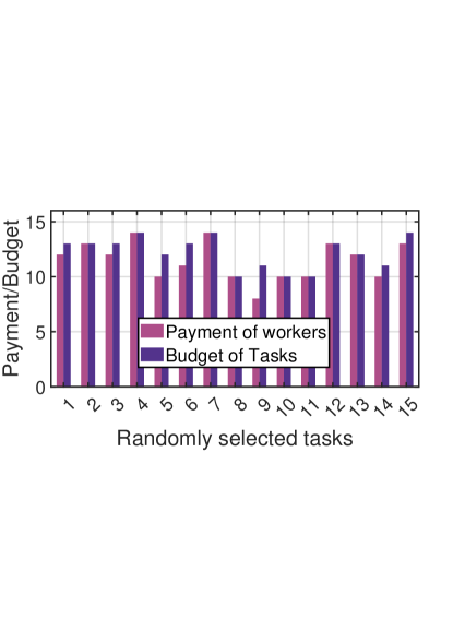
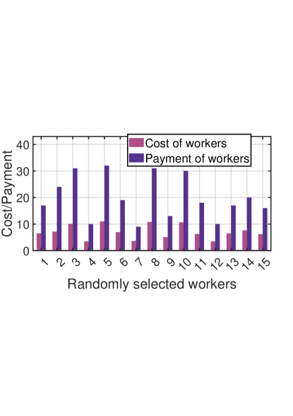
Figure 7: Performance comparisons in terms of individual rationality.

To demonstrate that our StagewiseTM³atch can support individual rationality, we randomly select 15 tasks (among 30 ones) and show their budgets along with the payments in Fig. 7(a). As we can see from Fig. 7(a), the total expenses of tasks that should be paid to workers consistently stay within their budgets, confirming that the set of matching mechanisms of StagewiseTM³atch method uphold the individual rationality of task owners. Also, Fig. 7(b) considers 15 randomly selected workers out of 30 ones, and shows the total service cost incurred on each worker never surpasses the total payments they receive, accordingly. Highlighting the individual rationality of workers.

References

- [1] J. Zhang, Y. Zhang, H. Wu, and W. Li, “An Ordered Submodularity-Based Budget-Feasible Mechanism for Opportunistic Mobile Crowdsensing Task Allocation and Pricing,” IEEE Trans. Mobile Comput., vol. 23, no. 2, pp. 1278-1294, 2024.
- [2] Y. Zhang, P. Li, T. Zhang, J. Liu, W. Huang, and L. Nie, “Dynamic User Recruitment in Edge-Aided Mobile Crowdsensing,” IEEE Trans. Veh. Technol., vol. 72, no. 7, pp. 9351-9365, 2023.
- [3] Y. Zhou, F. Tong, and S. He, “Bi-Objective Incentive Mechanism for Mobile Crowdsensing With Budget/Cost Constraint,” IEEE Trans. Mobile Comput., vol. 23, no. 1, pp. 223-237, 2024.
- [4] Y. Cheng, X. Wang, P. Zhou, X. Zhang and W. Wu, “Freshness-Aware Incentive Mechanism for Mobile Crowdsensing With Budget Constraint,” IEEE Trans. Serv. Comput., vol. 16, no. 6, pp. 4248-4260, 2023.
- [5] C. -L. Hu, K. -Y. Lin and C. K. Chang, “Incentive Mechanism for Mobile Crowdsensing With Two-Stage Stackelberg Game,” IEEE Trans. Serv. Comput., vol. 16, no. 3, pp. 1904-1918, 2023.
- [6] P. Sun, Z. Wang, L. Wu, Y. Feng, X. Pang, H. Qi, and Z. Wang, “Towards Personalized Privacy-Preserving Incentive for Truth Discovery in Mobile Crowdsensing Systems,” IEEE Trans. Mobile Comput., vol. 21, no. 1, pp. 352-365, 2022.
- [7] M. Xiao, Y. Xu, J. Zhou, J. Wu, S. Zhang, and J. Zheng, “AoI-aware Incentive Mechanism for Mobile Crowdsensing using Stackelberg Game,” IEEE Conf. Comput. Commun., 2023, pp. 1-10.
- [8] C. Dai, X. Wang, K. Liu, D. Qi, W. Lin, and P. Zhou, “Stable Task Assignment for Mobile Crowdsensing With Budget Constraint,” IEEE Trans. Mobile Comput., vol. 20, no. 12, pp. 3439-3452, 2021.
- [9] X. Tao, and A. S. Hafid, “DeepSensing: A Novel Mobile Crowdsensing Framework With Double Deep Q-Network and Prioritized Experience Replay,” IEEE Internet Things J., vol. 7, no. 12, pp. 11547-11558, 2020.
- [10] M. Liwang, X. Wang, and R. Chen, “Computing resource provisioning at the edge: An overbooking-enabled trading paradigm,” IEEE Wireless Commun., vol. 29, no. 5, pp. 68-76, 2022.
- [11] M. Liwang, Z. Gao, and X. Wang, “Let’s trade in the future! a futures-enabled fast resource trading mechanism in edge computing-assisted uav networks,” IEEE J. Select. Areas Commun., vol. 39, no. 11, pp. 3252-3270, 2021.
- [12] S. Sheng, R. Chen, P. Chen, X. Wang, and L. Wu, “Futures-based resource trading and fair pricing in real-time iot networks,” IEEE Wireless Commun. Lett., vol. 9, no. 1, pp. 125-128, 2020.
- [13] M. Liwang, and X. Wang, “Overbooking-empowered computing resource provisioning in cloud-aided mobile edge networks,” IEEE/ACM Trans. Netw., vol. 30, no. 5, pp. 2289-2303, 2022.
- [14] Q. Li, B. Niu, and L.-K. Chu, “Forward sourcing or spot trading? optimal commodity procurement policy with demand uncertainty risk and forecast update,” IEEE Syst. J., vol. 11, no. 3, pp. 1526-1536, 2017.
- [15] R. Chen, X. Wang, and X. Liu, “Smart futures based resource trading and coalition formation for real-time mobile data processing,” IEEE Trans. Serv. Comput., vol. 15, no. 5, pp. 3047-3060, 2022.
- [16] D. Li, C. Li, X. Deng, H. Liu, and J. Liu, “Familiar Paths Are the Best: Incentive Mechanism Based on Path-dependence Considering Space-time Coverage in Crowdsensing,” IEEE Trans. Mobile Comput., pp. 1-1, 2024.
- [17] H. Gao, H. Xu, C. Zhou, H. Zhai, C. Liu, M. Li, and Z. Han, “Dynamic Task Pricing in Mobile Crowdsensing: An Age-of-Information-Based Queueing Game Scheme,” IEEE Internet Things J., vol. 9, no. 21, pp. 21278-21291, 2022.
- [18] G. Ji, Z. Yao, B. Zhang, and C. Li, “Quality-Driven Online Task-Bundling-Based Incentive Mechanism for Mobile Crowdsensing,” IEEE Trans. Veh. Technol., vol. 71, no. 7, pp. 7876-7889, 2022.
- [19] Y. Ding, L. Zhang, and L. Guo, “Dynamic Delayed-Decision Task Assignment Under Spatial-Temporal Constraints in Mobile Crowdsensing,” IEEE Trans. Netw. Sci. Eng., vol. 9, no. 4, pp. 2418-2431, 2022.
- [20] X. Guo, C. Tu, Y. Hao, Z. Yu, F. Huang, and L. Wang, “Online User Recruitment With Adaptive Budget Segmentation in Sparse Mobile Crowdsensing,” IEEE Internet Things J., vol. 11, no. 5, pp. 8526-8538, 2024.
- [21] Y. Ye, H. Wang, C. H. Liu, Z. Dai, G. Li, G. Wang, and J. Tang, “QoI-Aware Mobile Crowdsensing for Metaverse by Multi-Agent Deep Reinforcement Learning,” IEEE J. Select. Areas Commun., vol. 42, no. 3, pp. 783-798, 2024.
- [22] J. Li, Y. Xiong, and J. She, “UAV Path Planning for Target Coverage Task in Dynamic Environment,” IEEE Internet Things J., vol. 10, no. 20, pp. 17734-17745, 2023.
- [23] S. T. Thant Sin, “The Parallel Processing Approach to the Dynamic Programming Algorithm of Knapsack Problem,” IEEE Conf. of Russian Young Researchers in Elect. Electron. Eng. (ElConRus), 2021, pp. 2252-2256.
- [24] H. Qi, M. Liwang, S. Hosseinalipour, X. Xia, Z. Cheng, X. Wang, and Z. Jiao, “Matching-Based Hybrid Service Trading for Task Assignment Over Dynamic Mobile Crowdsensing Networks,” IEEE Trans. Serv. Comput., pp. 1-1, 2023.
- [25] Y. Du, J. Li, L. Shi, T. Liu, F. Shu, and Z. Han, “Two-tier matching game in small cell networks for mobile edge computing,” IEEE Trans. Serv. Comput., vol. 15, no. 1, pp. 254-265, 2022.
- [26] T. Schaul, J. Quan, I. Antonoglou, and D. Silver, “Prioritized experience replay,” Proc. of the International Conference on Learning Representations (ICLR), 2016.
- [27] V. Mnih, K. Kavukcuoglu, D. Silver, A. A. Rusu, J. Veness, M. G. Bellemare, A. Graves, M. Riedmiller, A. K. Fidjeland, G. Ostrovski, S. Petersen, C. Beattie, A. Sadik, I. Antonoglou, H. King, D. Kumaran, D. Wierstra, S. Legg, and D. Hassabis, “Human-level control through deep reinforcement learning,” Nature, vol. 518, no. 7540, pp. 529-533, 2015.
- [28] F. Zou, L. Shen, Z. Jie, W. Zhang, W. Liu, “A Sufficient Condition for Convergences of Adam and RMSProp”, Proceedings of the IEEE/CVF Conference on Computer Vision and Pattern Recognition (CVPR), 2019, pp. 11127-11135.
- [29] “Taxi trips of chicago in 2013.” [Online]. Available: https://data.cityofchicago.org/Transportation/Taxi-Trips- 2013/6h2x-drp2
- [30] H. Qi, M. Liwang, X. Wang, L. Li, W. Gong, J. Jin, and Z. Jiao, “Bridge the Present and Future: A Cross-Layer Matching Game in Dynamic Cloud-Aided Mobile Edge Networks”, IEEE Trans. Mobile Comput., pp. 1-1, 2024.
- [31] J. Hu, Z. Wang, J. Wei, R. Lv, J. Zhao, Q. Wang, H. Chen, and D. Yang, “Towards Demand-Driven Dynamic Incentive for Mobile Crowdsensing Systems,” IEEE Trans. Wireless Commun., vol. 19, no. 7, pp. 4907-4918, 2020.
- [32] S. Luo, X. Chen, Q. Wu, Z. Zhou, and S. Yu, “Hfel: Joint edge association and resource allocation for cost-efficient hierarchical federated edge learning,” IEEE Trans. Wireless Commun., vol. 19, no. 10, pp. 6535-6548, 2020.