Cartan Quantum Metrology

Abstract

We address the characterization of two-qubit gates, focusing on bounds to precision in the joint estimation of the three parameters that define their Cartan decomposition. We derive the optimal probe states that jointly maximize precision, minimize sloppiness, and eliminate quantum incompatibility. Additionally, we analyze the properties of the set of optimal probes and evaluate their robustness against noise.

1 Introduction

The characterization of two-qubit gates is critical to any protocol in quantum information processing [1, 2, 3]. Two-qubit gates form the fundamental building blocks for universal quantum computation, enabling more complex operations through entanglement between qubits [4, 5, 6, 7]. Precise characterization of two-qubit gates enables the design of accurate gates, as even small errors can propagate and degrade the overall performance of quantum algorithms [8]. Furthermore, accurate gate characterization is essential for error correction protocols [9] and, in turn, for building fault-tolerant quantum computers [10] and scalable quantum systems.

The Cartan decomposition represents a powerful tool for analyzing generic two-qubit gates by breaking them down into simpler, more fundamental components [11, 12, 13, 14]. According to Cartan decomposition, any two-qubit gate can be expressed as a product of local single-qubit operations and a non-local part, known as the Cartan’s kernel. The kernel contains the essential entangling operations and is characterized by three independent parameters. Since local single-qubit operations can be efficiently controlled and do not contribute to entanglement, only the Cartan kernel is truly relevant for studying the gate’s features. In other words, the Cartan kernel captures the essential properties of the gate and simplifies the problem to the estimation of three parameters, which govern the non-local behavior of the gate.

In this paper, we address the joint estimation of the three Cartan parameters of a two-qubit gate [15, 16] by preparing an initial probe state, allowing it to interact with the gate, and then perform measurements on the resulting output state. Our goal is to optimize the encoding process so that all parameters are estimable, minimizing the sloppiness of the model while maximizing precision. Additionally, we aim to avoid any extra quantum noise that may arise from the non-commutativity of the measurements [17]. As we will demonstrate, it is possible to jointly achieve these three objectives, setting new benchmarks for the precise characterization of two-qubit quantum gates and providing insights into the precision-sloppiness tradeoff in qubit systems.

The paper is structured as follows. In Section 2 we introduce notation and the Cartan’s decomposition theorem applied to elements of $SU(4)$, whereas in Section 3 we briefly reviews the tools of multiparameter quantum metrology. In Section 4, we find the optimal states to achieve minimum sloppiness at fixed precision, whereas in Section 5 we assess the robustness of optimal probes in the presence of noise. Section 6 closes the paper with some concluding remarks.

2 Cartan decomposition

A generic state of a qubit system may be written in the Bloch representation as

$$\rho=\frac{1}{2}\left({\mathbb{I}_{2}}+\underline{r}\cdot\underline{\sigma}\right)\,,$$ (1)

where the Bloch vector $\underline{r}$ is given by

$$\underline{r}=\left(\text{Tr}[\sigma_{x}\rho],\text{Tr}[\sigma_{y}\rho],\text{Tr}[\sigma_{z}\rho]\right)^{T}\,,$$ (2)

and $\underline{\sigma}=(\sigma_{x},\sigma_{y},\sigma_{z})^{T}$ is the vector of Pauli matrices. The purity of the state $\rho$ is linked to the Bloch vector as

$$\mu[\rho]=\frac{1}{2}(1+|\underline{r}|^{2})\,.$$ (3)

Given $n$ qubits, the state of the whole system lives in the tensor product of the Hilbert spaces $\mathcal{H}^{n}=\bigotimes_{k=1}^{n}\mathcal{H}_{k}$. In the specific case of two qubits prepared in a pure state, we can use the concurrence as a measure of entanglement[18]. Given a generic state $\ket{\psi}=\sum_{x,y\in\{0,1\}}\alpha_{x,y}\ket{x}\ket{y}$ , the concurrence is defined as

$$\mathcal{C}(\ket{\psi})\equiv 2|\alpha_{00}\alpha_{11}-\alpha_{01}\alpha_{10}|.$$ (4)

This can be generalized for mixed states by $\mathcal{C}(\rho)\equiv\text{max}(0,\Lambda_{1}-\Lambda_{2}-\Lambda_{3}-\Lambda_{4})$, where $\Lambda_{1}\geq\Lambda_{2}\geq\Lambda_{3}\geq\Lambda_{4}$ are the eigenvalues of operator $R\equiv\sqrt{\sqrt{\rho}(\sigma_{y}\otimes\sigma_{y})\rho^{*}(\sigma_{y}\otimes\sigma_{y})\sqrt{\rho}}$.

Let us now consider a generic unitary gate acting on two qubits. Such an evolution corresponds to a linear operator in $SU(4)$. Élie Joseph Cartan proved the following theorem.

Theorem 2.1 (Cartan’s KAK decomposition).

Given a group $\underline{G}=\text{exp}(\underline{g})$, with a subgroup $\underline{K}=\text{exp}(\underline{k})$, and a Cartan subalgebra $\underline{a}$, where $\underline{g}=\underline{k}\oplus\underline{k}^{\perp}$ and $\underline{a}\subset\underline{k}^{\perp}$.
Then any $G\in\underline{G}$ can be written as $G=K_{1}AK_{2}$, with $K_{1},K_{2}\in\underline{K}$ and $A\in\text{exp}(\underline{a})$.

A special case of this theorem has been developed by Khaneja and Glaser for quantum computing. See [13] for a constructive proof using only linear algebra, of what is referred to as KAK1 theorem.

Theorem 2.2 (Khaneja and Glaser’s KAK1 theorem[11]).

Given any $S\in SU(4)$, there exists $A_{0},A_{1},B_{0},B_{1}\in SU(2)$, and $\underline{k}\in\mathbb{R}^{3}$, such that

$$S=(A_{1}\otimes A_{0})e^{i\underline{k}\cdot\underline{\Sigma}}(B_{1}\otimes B_{0})$$ (5)

where $\Sigma\equiv\left(\sigma_{x}\otimes\sigma_{x},\sigma_{y}\otimes\sigma_{y},\sigma_{z}\otimes\sigma_{z}\right)^{T}\equiv\left(\sigma_{XX},\sigma_{YY},\sigma_{ZZ}\right)^{T}$.

Starting from a generic operator over $\mathbb{C}^{4}$, which has 16 free components, unitarity reduces the degrees of freedom only by 1. One of the strengths of this theorem is the ability to separate the contribute of all these different parameters. In fact, what we see is that only 3 of the initial 15 parameters are involved in the interaction between the two qubits. The other 12 corresponds to single qubit evolutions. This decomposition is depicted in Fig. 1.

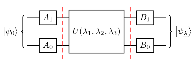
Figure 1: The decomposition of a generic gate into single qubit operations and a Cartan kernel.

The $U$ gate is referred to as the Cartan’s kernel, and will be the main object of our analysis. Using theorem 2.2 we may write the gate $U$ as

$$U=\exp\left\{-i\sum\limits_{j}\lambda_{j}\sigma_{j}\otimes\sigma_{j}\right\}\,,$$ (6)

which, in the standard basis, reads as follows (where $\lambda_{\pm}=\lambda_{1}\pm\lambda_{2}$)

$$U=\left(\begin{array}[]{cccc}e^{-i\lambda_{3}}\cos\lambda_{-}&0&0&-ie^{-i\lambda_{3}}\sin\lambda_{-}\\ 0&e^{i\lambda_{3}}\cos\lambda_{+}&-ie^{i\lambda_{3}}\sin\lambda_{+}&0\\ 0&-ie^{i\lambda_{3}}\sin\lambda_{+}&e^{i\lambda_{3}}\cos\lambda_{+}&0\\ -ie^{-i\lambda_{3}}\sin\lambda_{-}&0&0&e^{-i\lambda_{3}}\cos\lambda_{-}\\ \end{array}\right)\,.$$ (7)

Using instead the Bell basis ${\frac{1}{\sqrt{2}}\left\{\ket{00}+\ket{11},\ket{00}-\ket{11},\ket{01}+\ket{10},\ket{01}-\ket{10}\right\}}$, $U$ has the following diagonal form

$${U=\hbox{Diag}\left\{e^{-i(\lambda_{1}-\lambda_{2}+\lambda_{3})},e^{i(\lambda_{1}-\lambda_{2}-\lambda_{3})},e^{-i(\lambda_{1}+\lambda_{2}-\lambda_{3})},e^{i(\lambda_{1}+\lambda_{2}+\lambda_{3})}\right\}.}$$ (8)

The last thing to be discussed about the decomposition is the domain of the parameters. We initially have that $\lambda_{j}\in[0,2\pi)\in\mathbb{R}$. Then, we can define an equivalence relation, where two kernels $U,V\in SU(4)$ are said to be equivalent up to local operations, if there exists $R_{0},R_{1},L_{0},L_{1}\in U(2)$ such that $U=(R_{1}\otimes R_{0})V(L_{1}\otimes L_{0})$. It can be proven that this is a valid equivalence relation. Starting from this we can find three operations on $\underline{\lambda}$ that preserve the equivalence class. 1) Shift: $\underline{\lambda}$ can be shifted on any of the three components by an integer multiple of $\frac{\pi}{2}$. So given $n,m,l\in\mathbb{Z}$. $(\lambda_{1},\lambda_{2},\lambda_{3})\mapsto(\lambda_{1}+n\frac{\pi}{2},\lambda_{2}+m\frac{\pi}{2},\lambda_{3}+l\frac{\pi}{2});$ 2) Reverse: any two components can change sign. For example $(\lambda_{1},\lambda_{2},\lambda_{3})\mapsto(-\lambda_{1},-\lambda_{2},\lambda_{3})$; 3) Swap: any two components can be swapped. For example $(\lambda_{1},\lambda_{2},\lambda_{3})\mapsto(\lambda_{2},\lambda_{1},\lambda_{3})$. Using these operation it is possible to reduce the domain to what is called the canonical class vector set

$${{D_{C}}=\{\underline{\lambda}\in\mathbb{R}^{3}\ :\ \frac{\pi}{2}>\lambda_{1}\geq\lambda_{2}\geq\lambda_{3}\geq 0\wedge\lambda_{1}+\lambda_{2}\leq\frac{\pi}{2}\}}$$ (9)

For more details, see [13].

3 Multiparameter quantum estimation

The estimation of a single parameter or more than one have common features, but differ for fundamental reasons [19, 20]. The first one is that in quantum mechanics there may be observables which are incompatible, e.g., the observables employed to estimate two different parameters [16]. When this is the case, the joint estimation of the parameters is unavoidably affected by additional noise due to the non-commutativity of the measured observables. Additionally, there may be correlations between the parameters, or one of the parameter may be more relevant than the others, for the problem at hand. In all those cases, a weight matrix should be introduced to optimize precision under the given constraints.

In classical statistics, given a set of parameters to be estimated $\underline{\lambda}$, from the measurement of one or more observables $\underline{X}$, we have a conditional probability $p(\underline{x}|\underline{\lambda})$. The Fisher information matrix is defined by

$$F_{jk}=\sum\limits_{\underline{x}}\frac{\partial_{j}p(\underline{x}|\underline{\lambda})\ \partial_{k}p(\underline{x}|\underline{\lambda})}{p(\underline{x}|\underline{\lambda})},$$ (10)

where $\underline{x}$ denote the outcome(s) of the measurement of $\underline{X}$. We denote by $\underline{\hat{\lambda}}\equiv\underline{\hat{\lambda}}(\{x_{j}\})$, an estimator that maps the set of outcomes into the space of parameters. We also assume to work with unbiased estimators, meaning $\braket{\underline{\hat{\lambda}}}=\underline{\lambda}$. The covariance matrix of the estimator is given by $\text{Cov}[\underline{\hat{\lambda}}]_{jk}\equiv\braket{\hat{\lambda}_{j}\hat{\lambda}_{k}}-\braket{\hat{\lambda}_{j}}\braket{\hat{\lambda}_{k}}$ and the multiparameter classical Cramér-Rao bound [21] is the matrix inequality $\text{Cov}[\underline{\lambda}]\geq\frac{1}{M}F^{-1}$, where $M$ denotes the number of repeated measurements.

In order to build the analogue quantum Cramér-Rao bound, we first notice that for a quantum system, the conditional probability is given by the Born rule which, for pure states, reads $p(\underline{x}|\underline{\lambda})=|\braket{\underline{x}|\psi_{\underline{\lambda}}}|^{2}$. We then introduce the symmetric logarithmic derivative(SLD) of a parameter, which is implicitly defined by the relation [22]

$$\partial_{\lambda_{j}}\rho\equiv\partial_{j}\rho\equiv\frac{L_{\lambda_{j}}\rho+\rho L_{\lambda_{j}}}{2}\equiv\frac{L_{j}\rho+\rho L_{j}}{2},$$ (11)

where the subscript $j$ corresponds to the derivative with respect to the j-th parameter $\lambda_{j}$. In the case of pure states, the solution may be easily obtained by observing that $\rho^{2}=\rho$. We thus get

$$\partial_{j}\rho=\partial_{j}(\rho^{2})=(\partial_{j}\rho)\rho+\rho(\partial_{j}\rho)\,,$$ (12)

and comparing Eq. (11) to (12) we see that a solution is given by

$$L_{j}=2\partial_{j}\rho.$$ (13)

The quantum Fisher information matrix(QFIM) $[Q]_{jk}$ is then defined via the SLD by

$$Q_{jk}\equiv\text{Tr}\Big{[}\rho\frac{L_{j}L_{k}+L_{k}L_{j}}{2}\Big{]}=\frac{1}{2}\text{Tr}[\rho\{L_{j},L_{k}\}]\,$$ (14)

where $\rho$ is the state of the system. In general, it may be difficult to obtain the SLDs in operatorial form, and it is often convenient to express the QFIM in terms of the eigenvalues and eigenvectors of the statistical operator, as follows [15]

Theorem 3.1.

Given the spectral decomposition of a density matrix $\rho=\sum_{y_{j}\in S}y_{j}\ket{y_{j}}\bra{y_{j}}$, where $S=\{y_{j}\in\{y_{j}\}|y_{j}\neq 0\}$ is the support of non null eigenvalues. Then $Q_{jk}$ is given by

$$Q_{jk}= \sum\limits_{y_{l}\in S}\Big{(}\frac{(\partial_{j}y_{l})(\partial_{k}y_{l})}{y_{l}}+4y_{l}\hbox{\rm Re}[\braket{\partial_{j}y_{l}|\partial_{k}y_{l}}]\Big{)}$$

$$-\sum\limits_{y_{l},y_{m}\in S}\frac{8y_{l}y_{m}}{y_{l}+y_{m}}\text{\rm Re}[\braket{\partial_{j}y_{l}|y_{m}}\braket{y_{m}|\partial_{k}y_{l}}].$$ (15)

A useful expression for the QFIM may be obtained for pure states(i.e. $\rho_{\underline{\lambda}}=\ket{\psi}\bra{\psi}$), as follows

$$Q_{jk}=4\,\hbox{Re}[\braket{\partial_{j}\psi|\partial_{k}\psi}-\braket{\partial_{j}\psi|\psi}\braket{\psi|\partial_{k}\psi}].$$ (16)

The QFIM is an important object because it enters the quantum version of Cramèr-Rao bound, posing a lower bound on the covariance matrix of the estimators.

The Uhlmann curvature, also called incompatibility matrix is defined via the SLD, but instead of using the anticommutator as in Eq. (14), the commutator is used.

$$D_{jk}\equiv-i\text{Tr}\Big{[}\rho\frac{L_{j}L_{k}-L_{k}L_{j}}{2}\Big{]}=-\frac{i}{2}\text{Tr}[\rho[L_{j},L_{k}]]$$ (17)

From the definition we see that the main diagonal elements are always made of zeros. The meaning of the off diagonal terms is related to the quantum incompatibility. For $D=0$, all parameters are compatible, and the model is said to be asymptotically classical [16, 17]. In this case, the optimal estimation is asymptotically achievable via collective measurements. For pure states, we may write

$$D_{jk}=4\,\hbox{Im}[\braket{\partial_{j}\psi|\partial_{k}\psi}-\braket{\partial_{j}\psi|\psi}\braket{\psi|\partial_{k}\psi}].$$ (18)

As in the classical case, we denote by $\underline{\hat{\lambda}}\equiv\underline{\hat{\lambda}}(\{x_{j}\})$, an unbiased estimator that maps the set of outcomes into the space of parameters. The multiparameter Cramér-Rao bound states that

$$\text{Cov}[\underline{\lambda}]\geq\frac{Q^{-1}}{M}\,.$$ (19)

A scalar bound, limiting the overall precision of the multiparameter estimation strategy may be obtained by taking the trace of the above inequality, thus obtaining a bound on the sum of the variances of the estimators. By doing so we have

$$\text{Tr}\left[\text{Cov}[\underline{\lambda}]\right]{=}\sum_{j}\hbox{Var}\,\hat{\lambda}_{j}\geq\frac{\text{Tr}[Q^{-1}]}{M}\,.$$ (20)

The quantity $p=\text{Tr}[Q^{-1}]$ provides a lower bound to the optimal overall precision. As mentioned above, a weight matrix $W$ may be introduced in the definition of the precision $p=\text{Tr}[W\,Q^{-1}]$ to adjust the Cramér-Rao bound for specific applications. However, in our case, we set $W={\mathbb{I}}$ (the identity matrix) to emphasize that the three parameters of the Cartan kernel should be treated on the same foot since each one of them provide essential information on the nature of the two-qubit gate at hand.

In general, the bound in Eq. (20) is not achievable and a different scalar bound, termed Holevo bound [23] has been derived, which is achievable asymptotically. In our case, however, the two bounds coincide and therefore the quantity $p$ quantifies the overall precision of our scheme (see below for details).

Another feature of multi-parameter statistical models is that the encoding state may be not efficient, meaning that different parameters values are assigned locally to the same state and it is impossible to accurately recover them from the statistics of data. In these cases, the (classical or quantum) statistical model is termed sloppy [24, 25, 26, 27, 28, 29] and the (quantum) Fisher Information matrix is singular. This means that one or more parameters have zero (quantum) FI, and the statistical model is effectively only dependent on the other parameters. This may be seen explicitly by a reparametrization, not necessarily a linear one. The sloppiness of a statistical model may be quantified by the inverse of the determinant of the (quantum) Fisher Information matrix $s=1/\hbox{Det}\,Q$, and a relevant question in the analysis of a given model is whether there is a trade-off between precision and sloppiness or whether they can be jointly optimized, i.e., there exist conditions in which the trace of the inverse QFIM is minimum and the determinant of the QFIM is maximum.

To summarize, in our multiparameter model, $d=\hbox{Det}D$ quantifies the non commuting nature of the different SLDs and, in turn, the presence of additional noise of quantum origin. On the other hand, $p=\text{Tr}[Q^{-1}]$ quantifies the precision achievable in the joint estimation of the parameters, whereas $s=1/\hbox{Det}[Q]$ quantifies the sloppiness of the model, i.e. the degree of efficiency in the encoding of the parameter on the probe state. In the next Section, we will prove that in our case there are probe states leading to $d=0$, and thus no additional quantum noise is expected in the joint estimation of the Cartan parameter. Our goal will be therefore that of optimizing over the possible probe states in order to jointly minimize $p$ (i.e., maximize the precision) and $s$ (i.e., minimize sloppiness). Notice that the symmetric nature of the QFIM $Q$ already poses a bound on precision in terms of sloppiness. In fact, for a $n\times n$ real symmetric matrix $Q$, we have that $\hbox{Tr}[Q^{-1}]\geq n\,\hbox{Det}[Q]^{-1/n}$. In our $3\times 3$ case, this implies that

$$p\geq 3\,s^{1/3}\,.$$ (21)

We anticipate that the optimal probes found in the next Sections will allow us to saturate this bound.

4 Cartan metrology

In this Section, we address the estimation of the three parameters $\underline{\lambda}$ that characterize a Cartan gate of the form (6). In particular, we seek for the optimal achievable precision and for the probe states that allow one to achieve such precision. Additionally, we prove that incompatibility vanishes and analyze the tradeoff between precision and sloppiness of the statistical model. The quantum Fisher information is a convex function of the quantum state, which implies that the maximum QFI is achieved by pure states. Thus, restricting the analysis to pure states identifies the tightest possible Cramér-Rao bound. Due to the extended convexity of the Fisher information [30], the same is true for a two-qubit probe. Mixing two-qubit states cannot enhance the total QFI beyond the pure-state limit, and we thus assume that the two-qubit probe is prepared in a pure state.

4.1 Quantum Fisher information matrix and Uhlmann Curvature

To evaluate the QFIM we need the form of the state after the gate $\ket{\psi_{\underline{\lambda}}}\equiv U\ket{\psi_{0}}$ and, in turn, a parametrization of the initial state. In the canonical computational base, we have

$$\ket{\psi_{0}}\equiv\left(\alpha,\beta e^{i\phi_{\beta}},\gamma e^{i\phi_{\gamma}},\delta e^{i\phi_{\delta}}\right)^{T}\,,$$ (22)

with $\alpha,\beta,\gamma,\delta\in[0,1]$, and $\phi_{\beta},\phi_{\gamma},\phi_{\delta}\in[0,2\pi)$ such that $\alpha^{2}+\beta^{2}+\gamma^{2}+\delta^{2}=1$. From now on greek letters will correspond to the parametrization in the canonical base. Given the expression of the gate transformation $U$ in Eq. (7), we get

$$\ket{\psi_{\underline{\lambda}}}=\left(\begin{array}[]{c}e^{-i\lambda_{3}}\left[\alpha\cos(\lambda_{1}-\lambda_{2})-i\delta e^{i\phi_{\delta}}\sin(\lambda_{1}-\lambda_{2})\right]\\ e^{i\lambda_{3}}\left[\beta e^{i\phi_{\beta}}\cos(\lambda_{1}+\lambda_{2})-i\gamma e^{i\phi_{\gamma}}\sin(\lambda_{1}+\lambda_{2})\right]\\ e^{i\lambda_{3}}\left[\gamma e^{i\phi_{\gamma}}\cos(\lambda_{1}+\lambda_{2})-i\beta e^{i\phi_{\beta}}\sin(\lambda_{1}+\lambda_{2})\right]\\ e^{-i\lambda_{3}}\left[\delta e^{i\phi_{\delta}}\cos(\lambda_{1}-\lambda_{2})-i\alpha\sin(\lambda_{1}-\lambda_{2})\right]\\ \end{array}\right).$$ (23)

Using Eq. (16) we obtain the elements of the QFIM

$$\begin{split}&Q_{11}=4\Big{[}1-2\alpha\delta\cos\left(\phi_{\delta}\right)-2\beta\gamma\cos\left(\phi_{\beta}-\phi_{\gamma}\right)\Big{]}\Big{[}1+2\alpha\delta\cos\left(\phi_{\delta}\right)+2\beta\gamma\cos\left(\phi_{\beta}-\phi_{\gamma}\right)\Big{]}\\ &Q_{22}=4\Big{[}1-2\alpha\delta\cos\left(\phi_{\delta}\right)+2\beta\gamma\cos\left(\phi_{\beta}-\phi_{\gamma}\right)\Big{]}\Big{[}1+2\alpha\delta\cos\left(\phi_{\delta}\right)-2\beta\gamma\cos\left(\phi_{\beta}-\phi_{\gamma}\right)\Big{]}\\ &Q_{33}=16\left[\alpha^{2}+\delta^{2}\right]\left[\beta^{2}+\gamma^{2}\right]\\ &Q_{12}=Q_{21}=4\Big{[}-\alpha^{2}+\beta^{2}+\gamma^{2}-\delta^{2}+4\alpha^{2}\delta^{2}\cos^{2}\left(\phi_{\delta}\right)-4\beta^{2}\gamma^{2}\cos^{2}\left(\phi_{\beta}-\phi_{\gamma}\right)\Big{]}\\ &Q_{13}=Q_{31}=16\Big{[}\alpha\delta\left(\beta^{2}+\gamma^{2}\right)\cos\left(\phi_{\delta}\right)-\beta\gamma\left(\alpha^{2}+\delta^{2}\right)\cos\left(\phi_{\beta}-\phi_{\gamma}\right)\Big{]}\\ &Q_{23}=Q_{32}=-16\Big{[}\alpha\delta\left(\beta^{2}+\gamma^{2}\right)\cos\left(\phi_{\delta}\right)+\beta\gamma\left(\alpha^{2}+\delta^{2}\right)\cos\left(\phi_{\beta}-\phi_{\gamma}\right)\Big{]}\end{split}$$ (24)

Despite being seemingly complex, we get symmetrical and relatively simple expressions for its determinant, and the trace of its inverse

$$p =\frac{3}{16}\left(\frac{\alpha^{2}+\delta^{2}}{\alpha^{4}-2\alpha^{2}\delta^{2}\cos 2\phi_{\delta}+\delta^{4}}+\frac{\beta^{2}+\gamma^{2}}{\beta^{4}-2\beta^{2}\gamma^{2}\cos\left(2(\phi_{\beta}-\phi_{\gamma})\right)+\gamma^{4}}\right),$$ (25)

$$\frac{1}{s} =1024\left[\alpha^{4}+\delta^{4}-2\alpha^{2}\delta^{2}\cos 2\phi_{\delta}\right]\left[\beta^{4}+\gamma^{4}-2\beta^{2}\gamma^{2}\cos\left(2(\phi_{\beta}-\phi_{\gamma})\right)\right].$$ (26)

Notice that the trace of the inverse and the determinant of the QFIM are not functions of $\underline{\lambda}$, namely the statistical model is covariant. While this would have been a trivial result if the three generators were commuting operators, this is not the case in our problem. There are a few implications stemming from this fact. The first is that all the $\underline{\lambda}$’s can be estimated with the same precision. The same observation implies that this is true also for $\underline{\lambda}=\underline{0}$, i.e. for $U=\mathbb{I}$, showing that optimality is achievable independently of the fact that gate has or not an entangling power.

Using Eq. (17) we can calculate the Uhlmann curvature $D$, and by doing so we find that $D=0$. As mentioned above, this implies that our model is asymptotically classical, meaning that the CRB is asymptotically saturable. Additionally, this also tells us that the three parameters are compatible, and there is no additional noise due to quantum incompatibility.

4.2 State optimization

As a first step, we investigate how the trace of the inverse and the determinant of the QFIM are related by sampling numerically random states. The results are presented in Fig. 2, where points on the determinant-trace plane have been obtained sampling from a uniform distribution.

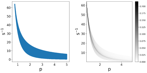
Figure 2: The trace-determinant region formed by uniformly sampling $2\cdot 10^{6}$ two-qubit states and using Eqs. (25) and (26). The left panel illustrates the physical region of the plane, while the right one shows the density of states. For graphical reasons the range of $p$ has been limited to values below 5 (the trace of the inverse QFIM is actually unbounded).

The first observation is that the sloppiness lies in the range $s\in[\frac{1}{64},\infty)$, while the range of precision is $p\in[\frac{3}{4},\infty)$. We also see that there are probe states leading to high values of the determinant (minimum sloppniness) and low values of the inverse of the trace (better precision), i.e., avoiding sloppiness is not necessarily decreasing precision. Indeed, the optimal point at $\left(\frac{3}{4},\frac{1}{64}\right)$ optimizes both quantities at the same time, also saturating the bound in Eq. (21).

To find the probe states that achieve that optimal condition, we can either minimize $p$ or $s$, since optimal states optimize both. To this aim, we rewrite Eq. (26) as follows

$$\begin{split}\text{Det}[Q]=1024&\Big{[}\left[\alpha^{2}+\delta^{2}\right]^{2}-2\alpha^{2}\delta^{2}\left[1+\cos\left(2\phi_{\delta}\right)\right]\Big{]}\times\\ &\Big{[}\left[\beta^{2}+\gamma^{2}\right]^{2}-2\beta^{2}\gamma^{2}\left[1+\cos\left(2(\phi_{\beta}-\phi_{\gamma})\right)\right]\Big{]}.\end{split}$$ (27)

The expression consists of two factors, each dependent on a different phase. In order to maximize the expression we can maximize the two factors using suitable phases. The last term in both factors is always negative, thus the maximum it can assume is $0$, when $\cos(x)=-1$. Alternatively, it may also be that either $\alpha$ or $\delta$, and either $\beta$ or $\gamma$ are $0$. These two options characterize two classes of solutions. Having cancelled the negative part, the terms $(\alpha^{2}+\delta^{2})$ and $(\beta^{2}+\gamma^{2})$ remains. Given this, a good change of variable that accounts for normalization is given by imposing $\alpha^{2}+\delta^{2}=\sin^{2}\theta$ and $\beta^{2}+\gamma^{2}=\cos^{2}\theta$. By doing so we get

$$\text{Det}[Q]=64\sin^{4}2\theta\,.$$ (28)

In this way, we confirm the numerical evidence and show that we have optimal states for $\sin 2\theta=1$. The optimal states are thus given by the two sets

$$\ket{\psi_{\text{sep}}} \in\Bigg{\{}\begin{pmatrix}\frac{1}{\sqrt{2}}\\ \frac{1}{\sqrt{2}}e^{i\phi}\\ 0\\ 0\end{pmatrix},\begin{pmatrix}\frac{1}{\sqrt{2}}\\ 0\\ \frac{1}{\sqrt{2}}e^{i\phi}\\ 0\end{pmatrix},\begin{pmatrix}0\\ \frac{1}{\sqrt{2}}e^{i\phi}\\ 0\\ \frac{1}{\sqrt{2}}\end{pmatrix},\begin{pmatrix}0\\ 0\\ \frac{1}{\sqrt{2}}e^{i\phi}\\ \frac{1}{\sqrt{2}}\end{pmatrix}\Bigg{\}}$$ (29)

$$\ket{\psi_{\text{ent}}} =\left(\alpha,\beta e^{i\phi},\pm i\sqrt{\frac{1}{2}-\beta^{2}}e^{i\phi},\pm i\sqrt{\frac{1}{2}-\alpha^{2}}\right)^{T}$$ (30)

with $\alpha,\beta\in[0,\frac{1}{\sqrt{2}}]$. The first class of solutions is made of factorized states, which are reducible to opportune combinations of the first qubit being in a superposition of 0 and 1 with equal probability, and the second one being either $\ket{1}$ or $\ket{0}$. The second class of solutions spans all possible concurrences from $0$ to $1$. We can see that the first class is actually contained in the second. Nevertheless, it is useful to keep them separate to study the effect of entanglement. Notice that the trace of the inverse QFIM may be written as $p=3/(4\sin^{2}2\theta)$, confirming that the optimal states in Eqs. (29) and (30), also minimize $p$.

4.3 Characterization of optimal states

We now proceed to ask if it is possible to more easily characterize optimal probe states. To this aim, it is useful to look again at $U$ in Eq. (7). We can see that if we block diagonalize $U$, we get 2 blocks of the form

$$M=e^{i\phi}\begin{pmatrix}\cos\theta&-i\sin\theta\\ -i\sin\theta&\cos\theta\end{pmatrix}\,,$$ (31)

i.e. represents a rotation $M=e^{i\phi}e^{-i\theta\sigma_{x}}$ along the $x$ axis on the Bloch sphere of an abstract qubit. Therefore our $U$ acts on those subspaces as a rotation, and the most sensible states are living on the $y-z$ plane of the corresponding Bloch sphere. With this observation in mind, we can now easily generate all optimal states, taking for example the state $\ket{0}$ and rotating it along the $x$ axis with $e^{i\theta\sigma_{x}}$

$$R_{x}(\theta)\ket{0}=e^{i\theta\sigma_{x}}\begin{pmatrix}1\\ 0\end{pmatrix}=\left(\begin{array}[]{c}\cos(\theta)\\ {-}i\sin(\theta)\\ \end{array}\right)=\left(\begin{array}[]{c}x\\ \pm i\sqrt{1-x^{2}}\\ \end{array}\right)$$ (32)

Taking this for the pairs $\alpha\sim\delta$ and $\beta\sim\gamma$, by combining them we get

$$\ket{\psi_{\text{ent}}}=\left(\alpha,\beta e^{i\phi},\pm i\sqrt{\frac{1}{2}-\beta^{2}}e^{i\phi},\pm i\sqrt{\frac{1}{2}-\alpha^{2}}\right)^{T}$$ (33)

which we recognize to describe exactly (all) the states in Eq. (30).

4.4 Entanglement is not a resource

Having found optimal solutions, we can now better assess whether entanglement plays any role in determining optimality of the probe states. To this aim, let us reconsider the data shown in Fig. 2, adding an equal number of factorizable states (orange).

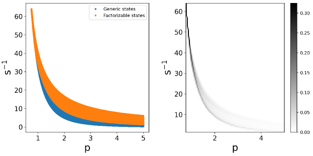
Figure 3: The left panel shows the distribution of states in the trace-determinant plane formed by uniformly sampling $2\cdot 10^{6}$ states (blue, no control on whether they are factorized or not), and $2\cdot 10^{6}$ factorizable states (orange). The right panel shows the density of factorizable states on the same plane. For graphical reasons the range of $p$ has been limited to values below 5 (actually the trace of the inverse QFIM is unbounded).

Results are shown in Fig. 3. What we see is that, despite not having anymore the lower part, we still get pretty much the same image and, once again, we have a higher density of states along the same curve. To complete the analysis we show in Fig. 4 how the trace of the inverse and the determinant of the QFIM are related to the concurrence of the probe. The plot shows that maximum precision is mostly achieved by probe states with small concurrence, while maximum sloppiness is mostly achieved by probes with large concurrence. Since every point in the image is reached by at least a state, it is clear that there is no relationship between optimality and entanglement.

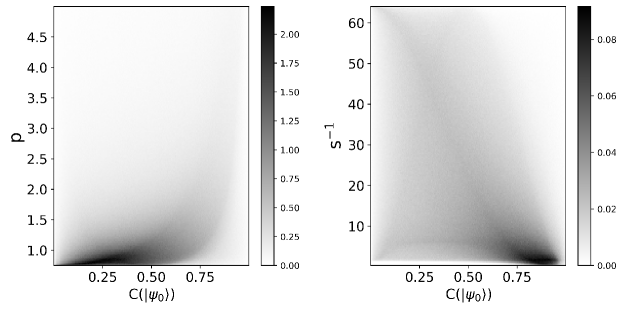
Figure 4: The left and right panels show the precision $p$ and the inverse of sloppiness $s^{-1}$ as a function of the concurrence of the probe state, respectively. The graphs are density maps built by sampling $2\cdot 10^{7}$ randomly generated states. This shows that precision and sloppiness are not related to the degree of entanglement of the probe state.

4.5 Probes that minimize sloppiness at fixed precision

Looking back at Fig. 2, we now want to characterize the states lying on the top curve, i.e., states minimizing sloppiness for a given level of precision (i.e., fixed $p$). We do this by rewriting the determinant as a function of $p$ and maximizing that function over the other parameters. The main problem in doing this in the standard basis is that we get complex equations. The derivation can be greatly simplified by switching to the Bell basis. We start by expressing the QFIM and the optimal states in the Bell basis. For convenience let’s rewrite $U$ in the Bell basis

$${U=\hbox{Diag}\left\{e^{-i(\lambda_{1}-\lambda_{2}+\lambda_{3})},e^{i(\lambda_{1}-\lambda_{2}-\lambda_{3})},e^{-i(\lambda_{1}+\lambda_{2}-\lambda_{3})},e^{i(\lambda_{1}+\lambda_{2}+\lambda_{3})}\right\}.}$$ (34)

We use latin letters to denote the amplitudes of a generic probe state in the Bell basis $\ket{\psi_{0}}=(a,be^{i\phi_{b}},ce^{i\phi_{c}},de^{i\phi_{d}})^{T}$, properly normalized. The evolved state after the application of $U$, is given by

$${\ket{\psi_{\underline{\lambda}}}=\left(\begin{array}[]{c}a\,e^{-i(\lambda_{1}-\lambda_{2}+\lambda_{3})}\\ b\,e^{i\left(\phi_{b}+\lambda_{1}-\lambda_{2}-\lambda_{3}\right)}\\ c\,e^{i\left(\phi_{c}-\lambda_{1}-\lambda_{2}+\lambda_{3}\right)}\\ d\,e^{i\left(\phi_{d}+\lambda_{1}+\lambda_{2}+\lambda_{3}\right)}\\ \end{array}\right)\,,}$$ (35)

and the elements of the QFIM by

$$\begin{split}&Q_{11}=16\left(1-b^{2}-d^{2}\right)\left(b^{2}+d^{2}\right)\\ &Q_{22}=16\left(1-b^{2}-c^{2}\right)\left(b^{2}+c^{2}\right)\\ &Q_{33}=16\left(1-c^{2}-d^{2}\right)\left(c^{2}+d^{2}\right)\\ &Q_{12}=Q_{21}=16\left(b^{4}+b^{2}\left(c^{2}+d^{2}-1\right)+c^{2}d^{2}\right)\\ &Q_{13}=Q_{31}=16\left(d^{2}-\left(b^{2}+d^{2}\right)\left(c^{2}+d^{2}\right)\right)\\ &Q_{23}=Q_{32}=16\left(c^{2}\left(b^{2}+d^{2}-1\right)+b^{2}d^{2}+c^{4}\right)\end{split}$$ (36)

which depend only on the real parameters $b,c,d$ and not on the phases. Solutions will then be defined up to relative phases applicable at the end. The precision $p$ and the determinant of the QFIM may be expressed as

$$p =\frac{3}{64}\left(\frac{1}{b^{2}}+\frac{1}{c^{2}}+\frac{1}{d^{2}}+\frac{1}{1-b^{2}-c^{2}-d^{2}}\right)$$ (37)

$$\frac{1}{s} =16384\left(1-b^{2}-c^{2}-d^{2}\right)^{2}b^{2}c^{2}d^{2}\,,$$ (38)

from which it is straightforward to obtain the optimal states

$${\ket{\psi_{\text{opt}}}=\frac{1}{2}\left(1,e^{i\phi_{b}},e^{i\phi_{c}},e^{i\phi_{d}}\right)^{T}\,.}$$ (39)

We now begin to look for optimal states at fixed precision. We express the amplitude $d\equiv d(b,c,p)$ in terms of precision arriving at

$$\frac{1}{s}=\frac{49152b^{4}c^{4}\left(1-b^{2}-c^{2}\right)}{b^{2}\left(64\,c^{2}p-3\right)-3c^{2}}.$$ (40)

The situation is illustrated in Fig. 5, where we show the determinant as a function of $b$ and $c$ at fixed $p$, taking into account the constraints on the domain.

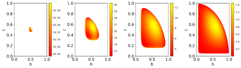
Figure 5: The four panels show the determinant of the QFIM as a function of $b$ and $c$ at different values of $p$. They are at respectively $p=0.76,1,2.5,20$.

The graphs show similar features for all values of $p$, and are characterized by 3 maxima. One is on the diagonal and the other two are on the edges of the domain (barely visible in the plots), sharing symmetrically one of the two components with the diagonal one. As a matter of fact, the function becomes more and more steep on the edges, making the yellow regions to nearly disappear, though the maxima are still there. Substituting a maximum in Eq. (40) we get

$$\frac{1}{s}=\frac{\left(8p-8\sqrt{\left(p-\frac{3}{4}\right)\left(p-\frac{3}{16}\right)}-3\right)\left(8p+8\sqrt{\left(p-\frac{3}{4}\right)\left(p-\frac{3}{16}\right)}+3\right)^{3}}{108p^{4}}$$ (41)

which expresses the minimum sloppiness achievable for a given precision $p$. To the leading around the minimum value of $p$, we have $1/s=64-512/3(p-3/4)+O(p-3/4)^{2}$. The corresponding (sub)optimal states, achieving those values of precision and sloppiness are given by

$$\ket{\psi_{\text{sub}}}=\left(\kappa_{2},\kappa_{1}e^{i\phi_{b}},\kappa_{1}e^{i\phi_{c}},\kappa_{1}e^{i\phi_{d}}\right)^{T}$$ (42)

with

$$\kappa_{1} =\frac{1}{4}\sqrt{\frac{8\sqrt{\left(p-\frac{3}{4}\right)\left(p-\frac{3}{16}\right)}+8p+3}{3p}}$$ (43)

$$\kappa_{2} =\frac{1}{4}\sqrt{\frac{-8\sqrt{\left(p-\frac{3}{4}\right)\left(p-\frac{3}{16}\right)}+8p-3}{p}}$$ (44)

where $\kappa_{2}$ can be switched in either of the four components.

5 Robustness against noise

Having found an entire class of optimal states, we now want to characterize their robustness against noise in the preparation stage. The circuits under consideration are shown in Fig. 6. We assume that after the preparation of the probe state one, or both channels may be subject to some form of noise before entering the gate. At this stage, we avoid classifying the states based on specific noise models, as these could be tied to particular implementations of the system [31]. Instead, our focus is on assessing the robustness and performance of the solutions obtained. To this aim, we apply some simple noise models and examine how optimal precision changes under these conditions. For simplicity, we have selected three distinct classes of probe states to illustrate how different optimal states respond to noise.

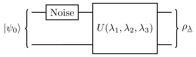
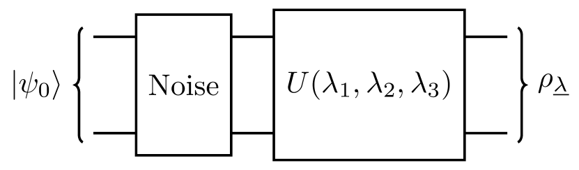
Figure 6: Quantum circuits representing how noisy channels alter the probe states before performing the $U$ evolution. We consider the action of the noisy channel on just one channel(left panel), and on both(right panel).

These classes are the following

$$\begin{split}\ket{\psi_{1}}&\equiv\begin{pmatrix}\frac{1}{\sqrt{2}}\\ \frac{1}{\sqrt{2}}e^{i\phi}\\ 0\\ 0\end{pmatrix}=\ket{0}\otimes\begin{pmatrix}\frac{1}{\sqrt{2}}\\ \frac{1}{\sqrt{2}}e^{i\phi}\end{pmatrix}\qquad\ket{\psi_{2}}\equiv\begin{pmatrix}\frac{1}{\sqrt{2}}\\ 0\\ \frac{1}{\sqrt{2}}e^{i\phi}\\ 0\end{pmatrix}=\begin{pmatrix}\frac{1}{\sqrt{2}}\\ \frac{1}{\sqrt{2}}e^{i\phi}\end{pmatrix}\otimes\ket{0}\\ \ket{\psi_{3}}&\equiv\begin{pmatrix}0.3\\ 0.2\ e^{i\phi}\\ i\sqrt{\frac{1}{2}-0.2^{2}}e^{i\phi}\\ i\sqrt{\frac{1}{2}-0.3^{2}}\end{pmatrix}.\end{split}$$ (45)

In particular, we consider the action of 1) bit flip noise, where the final state is given by

$$\rho_{\underline{\lambda}}=(1-\gamma)U\rho_{0}U^{\dagger}+\gamma U(\sigma_{x}\otimes\mathbb{I})\rho_{0}(\sigma_{x}\otimes\mathbb{I})^{\dagger}U^{\dagger}\qquad 0\leq\gamma\leq 1$$ (46)

if it acts only on one channel, and

$${\begin{split}\rho_{\underline{\lambda}}&=(1-2\gamma(1-\gamma)-\gamma^{2})U\rho_{0}U^{\dagger}++\gamma(1-\gamma)U(\sigma_{x}\otimes\mathbb{I})\rho_{0}(\sigma_{x}\otimes\mathbb{I})^{\dagger}U^{\dagger}\\ &+\gamma(1-\gamma)U(\mathbb{I}\otimes\sigma_{x})\rho_{0}(\mathbb{I}\otimes\sigma_{x})^{\dagger}U^{\dagger}+\gamma^{2}U(\sigma_{x}\otimes\sigma_{x})\rho_{0}(\sigma_{x}\otimes\sigma_{x})^{\dagger}U^{\dagger}\end{split}}$$ (47)

if it acts on both, and 2) the depolarizing noise, with the final state given by

$${\rho_{\underline{\lambda}}=(1-\gamma)U\rho_{0}U^{\dagger}+\frac{\gamma}{3}\sum\limits_{k\in\{x,y,z\}}U(\sigma_{k}\otimes\mathbb{I})\rho_{0}(\sigma_{k}\otimes\mathbb{I})^{\dagger}U^{\dagger}}$$ (48)

if it acts only on one channel, and

$$\rho_{\underline{\lambda}} =(1-\gamma)^{2}U\rho_{0}U^{\dagger}+(1-\gamma)\frac{\gamma}{3}\sum\limits_{k}U(\sigma_{k}\otimes\mathbb{I})\rho_{0}(\sigma_{k}\otimes\mathbb{I})^{\dagger}U^{\dagger}$$

$$+(1-\gamma)\frac{\gamma}{3}\sum\limits_{l}U(\mathbb{I}\otimes\sigma_{l})\rho_{0}(\mathbb{I}\otimes\sigma_{l})^{\dagger}U^{\dagger}+\frac{\gamma^{2}}{9}\sum\limits_{k,l}U(\sigma_{k}\otimes\sigma_{l})\rho_{0}(\sigma_{k}\otimes\sigma_{l})^{\dagger}U^{\dagger}$$ (49)

if it acts on both ($k,l\in\{x,y,z\}$). The precision is calculated using Eq. (15), and the overall goal is to see whether there exist probe states that maintain their sensitivity in the presence of noise. Results are summarized in Figs. 7 and 8, where we show precision as a function of the noise parameter $\gamma$ and the state parameter $\phi$ for the three classes of states defined in Eq. (45).

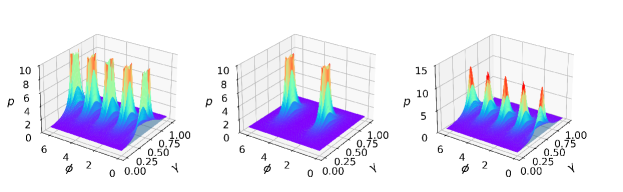
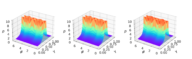
Figure 7: The precision $p$ as a function of the bit-flip noise parameter $\gamma$ and state parameter $\phi$. The upper panels illustrate results for the noise channel applied only on the second qubit, and the lower ones for the noise on both channels. The three columns are for the three classes of states in Eq. (45).

What we can see from Figs. 7 and 8 is that in all cases the function is convex for small $\gamma$ and thus robustness is ensured. Few additional remarks are in order: The first is that in the case of a single channel, for both errors there are phases for which the precision is comparable to the optimal one for every $\gamma$. This phases happens to be the same for $|\psi_{1}\rangle$ and $|\psi_{3}\rangle$ in the two cases shown, but in general they are error dependent. In fact, $|\psi_{2}\rangle$ shows some robust phases for the bit-flip noise, but none in the depolarizing case. Looking again at the single channel case, we can also see that the third state has bounded precision for any choice of $\phi$ and $\gamma$ for both kinds of errors. Lastly, we see how in the two channel case there are values of $\gamma$ for which the bound to precision diverges for all phases, for both error models. Notice also that in the limit $\gamma=1$ the noise channel corresponds to applying a unitary bit flip with unit probability, such that the pure input state gets mapped onto another optimal pure state. In this case, the bound to precision $p$ returns back to the minimum value $p=3/4$. This observation also explains the symmetry of the plot around the value $\gamma=1/2$.

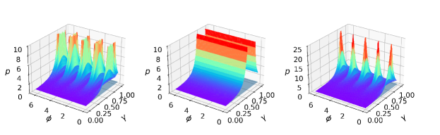
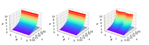
Figure 8: The precision $p$ as a function of the depolarizing noise parameter $\gamma$ and state parameter $\phi$. The upper panels illustrate results for the noise channel applied only on the second qubit, and the lower ones for the noise on both channels. The three columns are for the three classes of states in Eq. (45).

6 Discussion and conclusions

We have addressed the characterization of two-qubit gates, focusing on precision bounds in the joint estimation of the three parameters defining their Cartan decomposition. By considering a generic probe state at the input of the Cartan kernel, we identified classes of optimal probe states that maximize precision while minimizing sloppiness. For these probes, quantum incompatibility vanishes, allowing the three parameters to be estimated without any additional quantum noise. In addition, we have thoroughly analyzed the properties of these optimal probes and assessed their robustness against noise, revealing a subset of states that are more resilient to noise than others.

The optimal probes allow one to achieve a precision bound of $p=3/4$, meaning that the precision of any multidimensional set of estimators is constrained by $\sum_{j=1}^{3}\hbox{Var}\lambda_{j}\geq 3/4$. Furthermore, the same set of probes ensures the minimum sloppiness, $s=1/\text{Det}[Q]=1/64$. We have also determined the optimal precision-sloppiness tradeoff, providing the minimum value of $s$ for a fixed level of precision $p$. This tradeoff is given by:

$$s=\frac{108p^{4}}{\left(8p-8\sqrt{\left(p-\frac{3}{4}\right)\left(p-\frac{3}{16}\right)}-3\right)\left(8p+8\sqrt{\left(p-\frac{3}{4}\right)\left(p-\frac{3}{16}\right)}+3\right)^{3}}$$ (50)

with $p\in[3/4,+\infty)$

In conclusion, we have derived the optimal probe states to characterize the Cartan kernel of a generic two-qubit gate. These probes allow one to achieve maximum precision while eliminating quantum incompatibility. This enables noiseless, multidimensional, parameter estimation. These findings set a new benchmark for the precise characterization of two-qubit quantum gates, and shed light on the precision-sloppiness tradeoff in qubit systems.

References

- [1] B. Kraus, J. Cirac, Optimal quantum circuits for two-qubit gates, Physical Review A 63 (6) (2001) 062309. doi:10.1103/PhysRevA.63.062309.
- [2] G. Vidal, C. M. Dawson, Optimal quantum circuits for general two-qubit gates, Physical Review A 69 (1) (2004) 010301. doi:10.1103/PhysRevA.69.010301.
- [3] F. Vatan, C. Williams, Optimal realization of a generic two-qubit quantum gate, Physical Review A 69 (3) (2004) 032315. doi:10.1103/PhysRevA.69.032315.
- [4] A. Barenco, C. H. Bennett, R. Cleve, D. P. DiVincenzo, N. Margolus, P. Shor, T. Sleator, J. Smolin, H. Weinfurter, Elementary gates for quantum computation, Physical Review A 52 (5) (1995) 3457–3467. doi:10.1103/PhysRevA.52.3457.
- [5] Y. Makhlin, Nonlocal properties of two-qubit gates and mixed states, and the optimization of quantum computations, Quantum Information Processing 1 (2002) 243–252. doi:10.1023/A:1022144002391.
- [6] J. Zhang, J. Vala, S. Sastry, K. B. Whaley, Geometric theory of nonlocal two-qubit operations, Physical Review A 67 (4) (2003) 042313. doi:10.1103/PhysRevA.67.042313.
- [7] A. Rezakhani, Characterization of two-qubit perfect entanglers, Physical Review A—Atomic, Molecular, and Optical Physics 70 (5) (2004) 052313.
- [8] A. Gilchrist, N. K. Langford, M. A. Nielsen, Distance measures to compare real and ideal quantum processes, Physical Review A 71 (6) (2005) 062310. doi:10.1103/PhysRevA.71.062310.
- [9] C. H. Bennett, D. P. DiVincenzo, J. A. Smolin, W. K. Wootters, Mixed-state entanglement and quantum error correction, Physical Review A 54 (5) (1996) 3824–3851. doi:10.1103/PhysRevA.54.3824.
- [10] J. M. Chow, J. M. Gambetta, A. D. Córcoles, S. T. Merkel, J. A. Smolin, C. Rigetti, S. Poletto, G. A. Keefe, M. B. Rothwell, J. Rozen, M. B. Ketchen, M. Steffen, Universal quantum gate set approaching fault-tolerant thresholds with superconducting qubits, Physical Review Letters 109 (6) (2012) 060501. doi:10.1103/PhysRevLett.109.060501.
- [11] N. Khaneja, S. J. Glaser, Cartan decomposition of su(2) and control of spin systems, Chemical Physics 267 (1-3) (2001) 11–23. doi:10.1016/S0301-0104(01)00333-6.
- [12] V. V. Shende, I. L. Markov, S. S. Bullock, Minimal universal two-qubit controlled-not-based circuits, Physical Review A—Atomic, Molecular, and Optical Physics 69 (6) (2004) 062321.
- [13] R. R. Tucci, An introduction to cartan’s kak decomposition for qc programmers, arXiv preprint quant-ph/0507171 (2005).
- [14] C. Sparaciari, M. G. A. Paris, Canonical naimark extension for generalized measurements involving sets of pauli quantum observables chosen at random, Phys. Rev. A 87 (2013) 012106.
- [15] J. Liu, H. Yuan, X.-M. Lu, X. Wang, Quantum fisher information matrix and multiparameter estimation, Journal of Physics A: Mathematical and Theoretical 53 (2) (2019) 023001.
- [16] F. Albarelli, M. Barbieri, M. Genoni, I. Gianani, A perspective on multiparameter quantum metrology: From theoretical tools to applications in quantum imaging, Physics Letters A 384 (12) (2020) 126311.
- [17] S. Razavian, M. G. A. Paris, M. G. Genoni, On the quantumness of multiparameter estimation problems for qubit systems, Entropy 22 (11) (2020) 1197.
- [18] W. K. Wootters, Entanglement of formation and concurrence., Quantum Information and Computation 1 (1) (2001) 27–44.
- [19] G. Brida, I. P. Degiovanni, A. Florio, M. Genovese, P. Giorda, A. Meda, M. G. Paris, A. Shurupov, Experimental estimation of entanglement at the quantum limit, Physical review letters 104 (10) (2010) 100501.
- [20] M. G. A. Paris, Quantum estimation for quantum technology, International Journal of Quantum Information 7 (supp01) (2009) 125–137.
- [21] H. Cramér, Mathematical methods of statistics, Vol. 26, Princeton university press, 1999.
- [22] S.-i. Amari, H. Nagaoka, Methods of information geometry, Vol. 191, American Mathematical Soc., 2000.
- [23] A. Holevo, Commutation superoperator of a state and its applications to the noncommutative statistics, Reports on Mathematical Physics 12 (2) (1977) 251–271.
- [24] K. S. Brown, J. P. Sethna, Statistical mechanical approaches to models with many poorly known parameters, Physical review E 68 (2) (2003) 021904.
- [25] K. S. Brown, C. C. Hill, G. A. Calero, C. R. Myers, K. H. Lee, J. P. Sethna, R. A. Cerione, The statistical mechanics of complex signaling networks: nerve growth factor signaling, Physical biology 1 (3) (2004) 184.
-
[26]
J. J. Waterfall, F. P. Casey, R. N. Gutenkunst, K. S. Brown, C. R. Myers, P. W.
Brouwer, V. Elser, J. P. Sethna,
Sloppy-model
universality class and the vandermonde matrix, Phys. Rev. Lett. 97 (2006)
150601.
doi:10.1103/PhysRevLett.97.150601.
URL https://link.aps.org/doi/10.1103/PhysRevLett.97.150601 - [27] B. B. Machta, R. Chachra, M. K. Transtrum, J. P. Sethna, Parameter space compression underlies emergent theories and predictive models, Science 342 (6158) (2013) 604–607.
- [28] Y. Yang, F. Belliardo, V. Giovannetti, F. Li, Untwining multiple parameters at the exclusive zero-coincidence points with quantum control, New Journal of Physics 24 (12) (2023) 123041.
- [29] M. Frigerio, M. G. Paris, Overcoming sloppiness for enhanced metrology in continuous-variable quantum statistical models, arXiv preprint arXiv:2410.02989 (2024).
- [30] S. Alipour, A. T. Rezakhani, Extended convexity of quantum fisher information in quantum metrology, Physical Review A 91 (2015) 042104.
- [31] M. A. Rossi, C. Benedetti, M. G. Paris, Engineering decoherence for two-qubit systems interacting with a classical environment, International Journal of Quantum Information 12 (07n08) (2014) 1560003.