Demonstration of Fourier-domain Quantum Optical Coherence Tomography for a fast tomographic quantum imaging

Abstract

Using spectrally correlated photon pairs instead of classical laser light and coincidence detection instead of light intensity detection, Quantum Optical Coherence Tomography (Q-OCT) outperforms classical OCT in several experimental terms. It provides twice better axial resolution with the same spectral bandwidth and it is immune to even-order chromatic dispersion, including Group Velocity Dispersion responsible for the bulk of axial resolution degradation in the OCT images. Q-OCT has been performed in the time domain configuration, where one line of the two-dimensional image is acquired by axially translating the mirror in the interferometer’s reference arm and measuring the coincidence rate of photons arriving at two single-photon-sensitive detectors. Although successful at producing resolution-doubled and dispersion-cancelled images, it is still relatively slow and cannot compete with its classical counterpart. Here, we experimentally demonstrate Q-OCT in a novel Fourier-domain configuration, theoretically proposed in 2020, where the reference mirror is fixed and the joint spectra are acquired. We show that such a configuration allows for faster image acquisition than its time-domain configuration, providing a step forward towards a practical and competitive solution in the OCT arena. The limitations of the novel approach are discussed, contrasted with the limitations of both the time-domain approach and the traditional OCT.

Introduction

Quantum Optical Coherence Tomography (Q-OCT) was first proposed in 2002 Abouraddy et al. (2002) and then experimentally demonstrated in 2003 by the same group Nasr et al. (2003). It is a non-classical equivalent of conventional OCT, offering two times better axial resolution for the same spectral bandwidth and the elimination of the image-degrading even-order chromatic dispersion Abouraddy et al. (2002); Kolenderska et al. (2020a).

In the Q-OCT setup, conceptually presented in Fig. 1a, entangled photon pairs are generated in a nonlinear crystal and propagated in a Mach-Zehnder-type interferometer, called Hong-Ou-Mandel (HOM) interferometer Hong et al. (1987). While one of the photons is reflected from the object, the other photon propagates in the reference arm, both subsequently meeting at the beamsplitter. Each output port of the beam-splitter has a single-photon-sensitive detector enabling the measurement of coincidences (Fig. 1b), events in which the photons in the pair exit the beamsplitter using different ports and arrive at the detectors at the same time.

A dip in the coincidence signal occurs (Fig. 1c) when the reference arm length becomes equal to the object arm length. In such a situation, the photons arrive at the beam-splitter at the same time and - being indistinguishable (having the same optical parameters, e.g. the polarisation, central frequency) - they exit it using the same output port. This reduces the number of counted coincidences, providing a mechanism for detecting back-reflecting elements in the object inserted in the object arm. Such a depth structure of an object at a lateral position, called an A-scan, is mapped by varying the reference arm length and producing a dip whenever that length is matched to the length in the object arm set by an object layer.

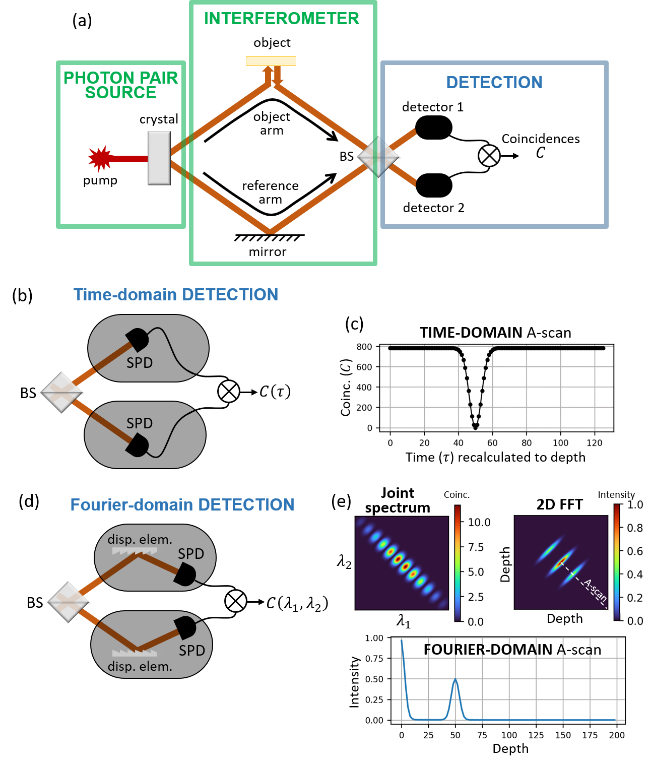
Figure 1: Quantum OCT comprises (a) a photon pair source, an interferometer where the produced photons propagate, and a detection part measuring coincidence $C$ of the photons’ arrival at two detectors. (b) The time-domain Q-OCT is based on single-photon-sensitive, single-pixel detectors, and outputs (c) a dip when the object arm length equals the reference arm length. (d) The Fourier-domain Q-OCT incorporates additional dispersive elements enabling wavelength discrimination, producing (e) a 2D joint spectrum which is Fourier transformed, with half the diagonal being the A-scan. BS - beamsplitter, $\lambda_{1}$, $\lambda_{2}$ - wavelength of the photons in the pair, SPD - single-photon-sensitive detector.

With a variable-length reference arm and single-pixel detection, Q-OCT has been realized in what is known in the OCT community as the time-domain configuration. Not only did this configuration show a twofold increase in axial resolution and chromatic dispersion cancellation for different photon pair sources and their spectral bandwidths (800 nm Hayama et al. (2022); Yepiz-Graciano et al. (2022); Sukharenko et al. (2021); Ibarra-Borja et al. (2019); Okano et al. (2015); Lopez-Mago and Novotny (2012); Nasr et al. (2009, 2004, 2003), 1550 nm Yepiz-Graciano et al. (2020); Graciano et al. (2019)), it proved to enable very useful modalities and extensions. Q-OCT was shown to perform polarisation-sensitive quantum imaging Sukharenko et al. (2021) and quantum optical coherence microscopy imaging Yepiz-Graciano et al. (2022).

Despite these advances, Q-OCT is still far from surpassing conventional OCT, mainly because of the method’s long measurement times. A good quality time-domain signal for a mirror requires about 1 second of integration time per data point, resulting in several minutes of acquisition time Yepiz-Graciano et al. (2022); Okano et al. (2015) per image line. The acquisition of a single image line is generally shorter for low-axial-resolution signals because the depth scan does not need to be very dense to properly sample the dips.

For a piece of glass, which is inherently much less reflective than a mirror, the integration time per data point increases to about 10 seconds and the image line acquisition time to hours, again depending on the axial resolution and additionally, on the thickness of the sample Yepiz-Graciano et al. (2022); Ibarra-Borja et al. (2019). Biological imaging with Q-OCT has only been successfully performed on objects coated with reflective particles, and the obtaining of a three-dimensional image took more than 24 hours Yepiz-Graciano et al. (2022); Nasr et al. (2009).

It has been noted that the acquisition time of Q-OCT could be reduced if advances in quantum technologies continue, allowing the use of brighter photon-pair sources or more sensitive and less noisy single-photon detectors Teich et al. (2012). Alternatively, time-optimised measurement schemes could be explored, with such a scheme already proposed in 2019 Ibarra-Borja et al. (2019). Inspired by conventional OCT, the full-field approach, in which all lines of the image are acquired simultaneously, allowed a two-dimensional en face image to be obtained in 3 minutes. Another notable advancement in this area came just one year later from the same research group Yepiz-Graciano et al. (2020). Taking a leaf out of the conventional OCT book again, U’Ren & Cruz-Ramirez et al. proposed in early 2020 a partial shift in the Q-OCT detection to the Fourier domain. By measuring a one-dimensional spectrum for a given reference arm length and using it to reconstruct the time-domain signal, the acquisition of a single image line for extended objects was reduced from hours to minutes.

We also explored the potential of Fourier-domain measurements as a more rapid detection alternative for Q-OCT. This was initially presented at the European Conference on Biomedical Optics in June 2019 Kolenderska et al. (2019) and subsequently elaborated upon in a theoretical journal article published the following year Kolenderska et al. (2020b). In our approach, we proposed a complete shift to the Fourier domain by measuring a whole two-dimensional joint spectrum, as opposed to its single diagonal as is the case in the work of U’Ren & Cruz-Ramirez et al. Yepiz-Graciano et al. (2020). A joint spectrum is obtained by counting the coincidence events in the output ports of the final beamsplitter, as is done in the time-domain modality. However, in this approach, photons in each port undergo wavelength measurement(Fig. 1d) enabling the detected coincidences to be plotted as a function of two wavelengths (Fig. 1e). The resulting joint spectrum is Fourier transformed and half its diagonal is taken to produce an A-scan Kolenderska and Szkulmowski (2021).

Here we present an experimental setup for Fourier-domain Q-OCT, where the joint spectral detection is realised with two 5-kilometre-long fibre coils and superconducting single photon detectors. Such a Fourier-domain Q-OCT allows for a much faster depth scan without any moving elements in the reference arm. With a spectrally broadband laser as the pump, the joint spectrum allows the artefacts, the parasitic elements in the signal that do not correspond to the structure, to be dealt with efficiently. We propose an interpolation-based algorithm for compensating the joint spectrum distortions caused by the fibre coil dispersion, inspired by OCT’s spectral calibration algorithms. Also, a coincidence post-selection algorithm is developed and applied for efficient, error-free extraction of an A-scan from experimental joint spectra. Based on a mirror and pieces of glass and plastic as objects, we compare the artefact removal capabilities as well as general imaging parameters (axial resolution, imaging range) of Fourier-domain Q-OCT imaging with that of the time-domain one. Comparison with traditional OCT shows the problems that need to be solved for Q-OCT to become a useful alternative.

Methods

The experimental setup

The Fourier-domain Quantum Optical Coherence Tomography (Fd-Q-OCT) setup consists of three parts: the photon pair source, the interferometer, and the joint spectral detection, marked by rectangles in the setup schematic in Fig. 2.

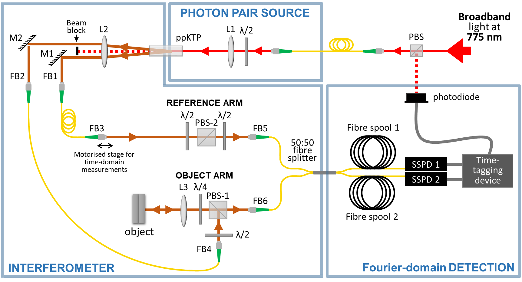
Figure 2: Fourier-domain Quantum OCT setup uses broadband laser light at 775 nm, Coherent Chameleon Ultra+, 80 MHz repetition rate, 10 nm bandwidth, to pump the ppKTP, 24.7 $\mu$m poling period, crystal and generate photon pairs at 1550 nm. One photon from the pair propagates in the object arm where it is reflected from the object. The other photon from the pair propagates in the reference arm, whose length and produced polarisation match those of the object arm. The photons overlap at the 50:50 fibre splitter where they quantum interfere. The wavelength-dependent coincidence rate is measured using two fibre spools, superconducting single-photon detectors SSPDs, Scontel, and a photodiode-triggered time-tagging device, Qutag by Qutools. A time-domain Quantum OCT signal is acquired by translating the motorised stage in the reference arm. Conventional OCT is performed by connecting a second fibre splitter to a Menlo T-light laser (central wavelength of 1550 nm and the total bandwidth of 160 nm) at one end and to FB1 and FB2 at the other one. The classical fringes are then acquired using an optical spectrum analyser, Yokogawa AQ6374E, connected to one of the output ports of the 50:50 fibre splitter. M1-2 – mirrors, L1-3 – lenses (f=125 mm, 75 mm, 50 mm), $\lambda$/2 – half-wave plate, $\lambda$/4 – quarter-wave plate, PBS - polarisation beamsplitter, fibre connectors: FB1 and FB2 – 8-mm focal length lenses in front of HP1550 single-mode fibres, FB3 and FB4 – collimation package, Thorlabs FC1550-f6.37 mm, FB5 and FB6 – lens with f=11 mm in front of the fibres.

In the photon pair source, a pulsed laser light with a central wavelength of 775 nm is used as the pump for the Spontaneous Parametric Down Conversion (SPDC) process in which entangled photon pairs are created. The pump light is focused by a lens L1 onto a ppKTP crystal, and two photons with wavelengths around 1550 nm and polarisations identical to that of the pump photon exit the crystal in different directions, consequently realising non-collinear, type 0 SPDC. The half-wave plate situated in front of L1 adjusts the polarisation of the pump beam for the optimum pair production rate.

The two photons exiting the crystal in different directions form two arms of the interferometer. After passing through the collimating lens L2, the photons are reflected by mirrors M1 and M2 and then coupled into separate fibres FB1 and FB2. While the photons entering FB1 propagate in the reference arm, the photons entering FB2 propagate in the object arm. In both arms, light is output to free space with matching light collimation packages FB3 and FB4 and injected back into fibres with matching injection setups FB5 and FB6.

In the object arm, the first half-wave plate rotates the polarisation of the light to maximise reflection at the polarising beam-splitter PBS-1, thereby directing most of the light towards the object. The L3 achromatic lens focuses the light onto the object and the quarter-wave plate ensures that most of the light reflected from the object is transmitted through PBS-1. The polarisation optics in the reference arm ensure that the polarisation states of the photons are the same at the input of the 50:50 fibre splitter. To this end, the first half-wave plate maximises transmission through the polarisation beam-splitter PBS-2, ensuring the same polarisation as the one at the output of the object arm’s PBS-1. The second half-wave plate in the reference arm is added to pre-compensate for any polarisation mismatch caused by the input fibre of the 50:50 fibre splitter. All the fibres were taped to the optic table to prevent them from moving and affecting the polarisation.

The 50:50 fibre splitter is the beam splitter where the photons overlap and quantum interfere when the object arm length is equal to the reference arm length. The two outputs of the fibre splitter are connected to 5-kilometre-long single-mode fibre spools where the photons are delayed in a wavelength-dependent manner due to chromatic dispersion. A time-tagging device provides information on the arrival time of the photons at the Superconducting Single-Photon Detectors, with the reference point provided by the photodiode illuminated by the pulsed pump light. The time window in which the detectors wait for photons is equal to the repetition time of the pump laser, and the clock in the time-tagging device is triggered with the rising slope of the signal from the photodiode.

The time-domain Q-OCT measurement is performed by sequentially translating the motorised stage at the FB3 position and recording the total number of coincidences within the acquisition time window at each position. The fibre spools are not disconnected when performing the time-domain measurements.

Conventional OCT uses a pulsed laser with a centre wavelength of 1550 nm. It is fed into an input port of a second 50:50 fibre splitter whose output ports are connected to FB1 and FB2. The classical fringes are detected using an optical spectrum analyser (OSA) connected to one of the output ports of the existing 50:50 fibre splitter.

Data processing

A joint spectrum - the signal acquired in Fourier-domain Q-OCT - possesses imperfections which are addressed with two algorithms. Whereas the interpolation-based linearisation algorithm targets nonlinear distribution of the fringes occurring due to the fibre spools’ chromatic dispersion, the coincidence post-selection algorithm optimises the extraction of an A-scan, ensuring no information loss due to noise or non-central signal location on the 2D joint spectral plane.

To visualise data processing steps, a mirror was placed as an object in the object arm and a joint spectrum was measured approximately 0.37 mm away from the zero optical path difference in the interferometer, with the acquisition time of 10 seconds. As shown in Fig. 3a, the acquired joint spectrum is oval-shaped and located diagonally, with a single-frequency modulation distributed in the diagonal direction as well. There is a cross-like component with a bright centre on the left, most probably related to the pump light leakage.

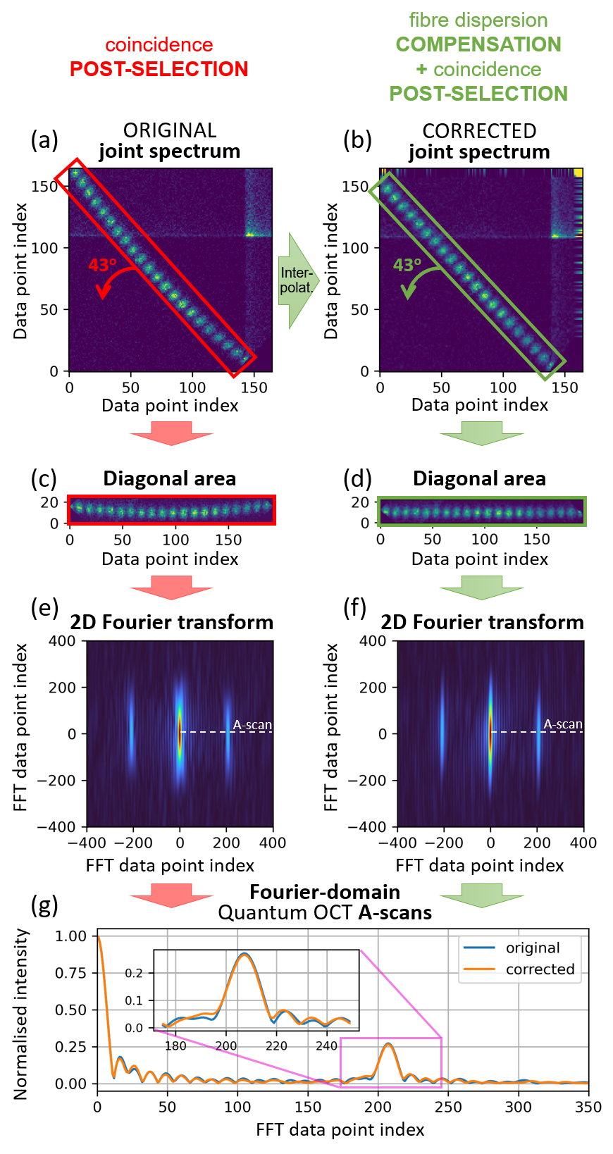
Figure 3: Measurement for a mirror as an object. (a) The acquired joint spectrum shows a diagonally-oriented single-frequency modulation which is bent due to the dispersion of the detection’s fibre spools. (b) After interpolation, the joint spectrum is straightened diagonally. Coincidence post-selection data processing is performed to extract (c) the diagonal area of the original joint spectrum, and (d) the diagonal area of the fibre-dispersion-corrected joint spectrum. (e), (f) 2D Fourier transforms of the extracted portions incorporate a central zero-frequency peak, a structural peak and its twin at the other side of the zero-frequency peak. (e) Comparison of the A-scans extracted from both Fourier transforms shows no significant difference.

Linearisation. Due to the chromatic dispersion of the 5-kilometre-long fibre spools used in the detection system, the joint spectrum is slightly bent. To correct this non-uniformity, the joint spectrum is interpolated in a manner very similar to how lambda-to-$k$ calibration is done in the OCT field Wang and Ding (2008); Szkulmowski et al. (2016). Such an approach was chosen because the effect compensated with the lambda-to-$k$ calibration in OCT and the effect observed here are similar. Whereas in conventional OCT (more specifically, its spectral domain version) the acquired one-dimensional spectrum is nonlinearly sampled in $k$ due to linear-in-lambda light dispersing at the diffraction grating, the joint spectrum in Fd-Q-OCT is nonlinearly sampled due to the non-zero dispersion of the fibre spools. In conventional OCT, lambda-to-$k$ calibration recovers the linear sampling and is performed by shifting the measured intensity values to fractional indices using interpolation.

Here, we apply this linearisation approach by first interpolating all rows of the joint spectrum, and then all columns of the joint spectrum. The vector with fractional indices is calculated using the function $A=A(i)$, where $i$ is the index of the X or Y axis. $A=A_{1}i^{2}+A_{2}i+C$, with $A_{1}=-0.001$, $A_{2}=1$ and $A_{2}=0$ chosen so that the maximum value in the sum of the diagonals is maximal. The interpolation vector is the same for both rows and columns because due to the symmetricity of the detection, the amount of dispersion to correct for is very similar for both detection channels. As observed in Fig. 3b, such interpolation-based fibre dispersion correction leads to a straightening of the joint spectrum.

A-scan extraction should involve Fourier transforming the joint spectrum and extracting the resulting Fourier transform’s diagonal, as suggested in Fig. 1e, but we decided to insert two additional steps: rotation and area selection. Called coincidence post-selection data processing, it guarantees precise information retrieval from the acquired joint spectra.

Step one, rotation, ensures that the main diagonal of the joint spectrum is extracted. One can notice that the acquired joint spectra are not distributed on the same number of points in the X and Y direction (see Fig. 3a, where the joint spectrum covers less than 150 points in the X direction, but more than 150 points in the Y direction), and consequently, taking the diagonal of such a data structure would not provide the diagonal of the joint spectrum. That is why, before Fourier transforming, the joint spectrum is first rotated so that the fringes distribution is flat. This is done in Python using the "rotate" method from SciPy library. The rotation angle is 43 degrees, which confirmed our concerns in this matter: if the joint spectrum is spread equally on both axes, the rotation angle that would ensure a flat distribution would be 45 degrees.

Step two, area selection, removes the influence of both dark and random coincidences, especially the ones induced by the pump (the cross-like structure observed in Fig. 3a or b). Only the area containing the fringes is taken (Fig. 3c in the case of the original joint spectrum, Fig. 3d in the case of the fibre-dispersion-corrected spectrum) and Fourier transformed. The resulting 2D Fourier transforms, presented in Fig. 3e and f, show a central, zero-frequency peak, and two symmetrically located peaks, one being the structural peak corresponding to the mirror and the other one being its twin and appearing due to Fourier transformation’s inherent inability to discern between positive and negative frequencies.

Uncompensated fibre dispersion leads to peak distortions in the 2D Fourier transform as observed in Fig. 3e, whereas the 2D Fourier transform calculated from the fibre-dispersion-corrected joint spectrum incorporates sharp, Gaussian-shaped elements (Fig. 3f). We note that all the peaks are narrow in the horizontal direction due to the large horizontal width of the rotated joint spectrum (being the diagonal width of the input joint spectrum), and broad in the vertical direction due to the small vertical width of the rotated joint spectrum (being the anti-diagonal width of the input joint spectrum).

A-scans are extracted from both original and corrected 2D Fourier transforms by taking half of their most central row (which correspond to the joint spectrum’s diagonal), and plotted together in Fig. 3g in blue and orange lines, respectively. One would intuitively expect that the fibre dispersion correction would lead to the improvement (i.e. decrease) of the peak’s width since, as experienced in conventional OCT, the nonlinearity caused by dispersion leads to peak broadening. No difference in the signal shape, let alone the peak width, is observed, because the uniformity of the fringes distribution is not affected by the fibre dispersion. The distribution of the fringes can only be modulated in the interferometer due to dispersion mismatch between the interferometer arms. Because even-order dispersion is cancelled, the only change to the fringes’ distribution can come from odd-order dispersion mismatch which is negligible in this case (no peak distortion is observed). Fibre dispersion compensation is further analysed in terms of its influence on the imaging performance in the next subsection, called "Axial resolution and imaging range".

Results

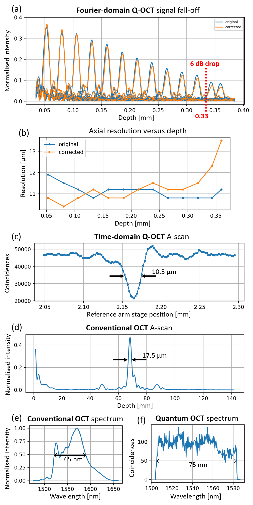
Figure 4: (a) A-scans retrieved from the joint spectra acquired for 13 different reference arm lengths let estimate the effective imaging depth to be around 0.33 mm for both the fibre-dispersion-corrected case (orange), and the uncorrected, original case (blue). (b) The axial resolution is uniform if the original data is used (blue), but is improved with a slight decrease after the 6 dB fall-off is reached when the same data is fibre-dispersion-corrected (orange). (c) The axial resolution is 10.5 $\mu$m when the signal is acquired in the time domain. (d) As expected, the axial resolution is worse in the conventional OCT, 17.5 $\mu$m, with (e) conventional OCT spectrum having a spectral bandwidth of 65 nm, similar to (f) the diagonal width of the joint spectrum, 75 nm.

Axial resolution and imaging range

To assess the axial resolution and imaging range of the Fd-Q-OCT setup, the joint spectrum was acquired for 13 different lengths of the reference arm with the mirror as an object in the object arm. The joint spectra were processed into A-scans which when plotted together in Fig. 4a show the signal fall-off, i.e. depth-dependent sensitivity decay due to detection’s finite spectral resolution. The blue peaks in Fig. 4a are obtained when the acquired joint spectra undergo coincidence post-selection data processing directly (the red path in Fig. 3), and the orange peaks are obtained when the same joint spectra are first fibre dispersion corrected before processed with the coincidence post-selection algorithm (the green path in Fig. 3).

One can see in Fig. 4a that the effective imaging range, defined as the depth at which a 6-dB drop in the peak height occurs, is around 0.33 mm in both cases. Interestingly, the height of the dispersion-uncorrected peaks looks slightly better than in the case of the fibre-dispersion-corrected ones.

The axial resolution is around 11 $\mu$m in both cases. As seen in Fig. 4b, while the axial resolution is quite uniform depth-wise for the dispersion-uncorrected case (blue line), it is a little better for the dispersion-corrected case, with a slight decrease observed for larger depths. The signal fall-off and the depth-dependent axial resolution further confirm no advantage to performing fibre dispersion compensation other than easier interpretation of the results, i.e. identification of the artefact elements in the 2D Fourier transforms. This is why, since the quality difference between the corrected and uncorrected A-scans is negligible, for the remainder of the article the fibre-dispersion-corrected results will be shown for the sole purpose of the ease of 2D Fourier transform interpretation. These surprising results - certainly necessitating a separate, in-depth investigation - are further commented on in the Summary and discussion section.

The axial resolution in Fourier-domain Q-OCT is compared to the axial resolutions obtained using the time-domain approach and conventional OCT with similar spectral bandwidth. The time-domain signal was acquired by changing the length of the reference arm with a step size equal to 1 $\mu$m, and acquiring the coincidences (Fig. 4c). The resulting dip’s full width at half maximum (FWHM) is 10.5 $\mu$m.

The conventional OCT spectrum was acquired, nonlinearity-corrected using the algorithms from Ref. Wang and Ding (2008) and Fourier transformed. The resulting A-scan, presented in Fig. 4d, shows a peak whose FWHM - representing the axial resolution - is approximately 17.5 $\mu$m. As already shown both theoretically and experimentally, the conventional OCT axial resolution is worse than that obtained with Q-OCT for the same spectral bandwidth. In our case, the increase of the axial resolution is not exactly two times, because of slight differences between the spectral bandwidth of the laser. It is approx. 65 nm, see the spectrum in Fig. 4e, and the diagonal width of the joint spectrum is approx. 75 nm, see Fig. 4f.

A single joint spectrum behind Fig. 4 was acquired in 10 seconds. Each point in the time-domain signal was acquired for 1 second, resulting in a total acquisition time of around 2 minutes. Please see Tab. 1 for the comparison. The conventional OCT spectrum was measured using the OSA in under a second which is considered rather long when compared to the acquisition times achieved by standard OCT machines.

Single-layer glass

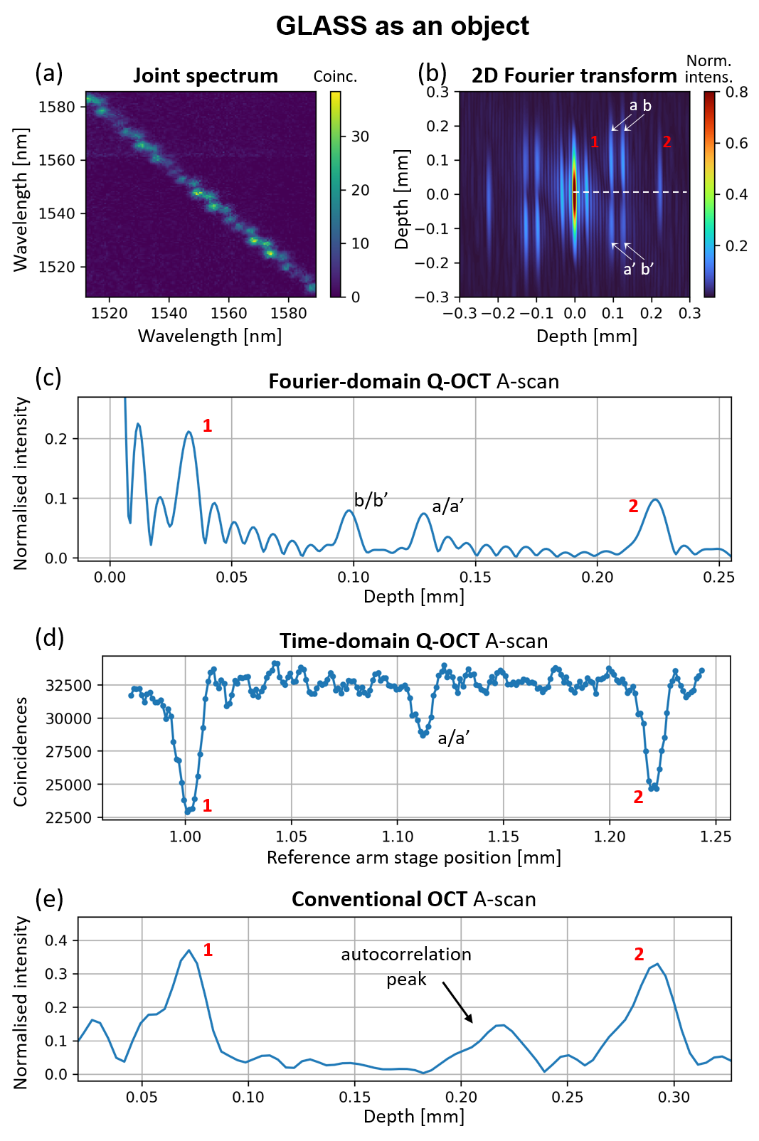
Figure 5: Measurement of a glass sample. (a) Fibre-dispersion-corrected joint spectrum produces (b) 2D Fourier transform with sharp, undistorted peaks: two corresponding to the structure of the imaged glass (1,2) and four being the artefacts (a, a’ and b,b’). (c) The extracted Fourier-domain A-scan shows both structural peaks and two artefact peaks b/b’ and a/a’. (d) The time-domain A-scan shows structural dips as well as an artefact, and (e) the conventional OCT A-scan shows the structure of the object with a lower resolution and with an autocorrelation peak.

Using glass as an object gives more insight into the appearance of the artefacts, i.e. the peaks that do not correspond to the structure of the imaged object. Fig. 5a and Fig. 5b show the fibre-dispersion-corrected joint spectrum for a 100-$\mu$m-thick glass, acquired in 3 minutes, and its 2D Fourier transform, respectively.

In the 2D Fourier transform, one can discern the zero-frequency peak in the centre and two structural peaks (marked with 1 and 2 in Fig. 5b) located in the central row which corresponds to the joint spectrum diagonal. There are four additional peaks situated symmetrically around the central row, a and its twin a’ at the midpoint between the structural peaks and b and its twin b’ at the distance from the zero-frequency peak equal to half the glass thickness. The same set of peaks appears in the other half of the 2D Fourier transform just as in the case of the mirror.

The artefact peaks associated with a/a’ and b/b’ are clearly visible in the Fourier-domain A-scan (Fig. 5c) extracted from the 2D Fourier transform. This is due to the fact that a and a’ (as well as b and b’) overlap the main diagonal of the 2D Fourier transform.

For reference, a time-domain signal (Fig. 5d) was acquired by counting coincidence events for a range of reference stage positions (2.5 $\mu$m step, 10 seconds integration per data point, resulting in over 30-minute total acquisition time). Such a time-domain A-scan incorporates dips corresponding to the glass structure (1 and 2 in Fig. 5d). As expected, there is an additional, artefact dip at the midpoint between the structural dips.

The conventional OCT A-scan, in Fig. 5e, shows both peaks as well as an autocorrelation peak, which is a peak appearing due to the interference of light reflected from the objects’ surfaces. Naturally, the structural peaks’ width is larger than that of the peaks and dips in Q-OCT signals. The conventional OCT spectrum was acquired using the OSA in less than a second. See Tab. 1 for the performance comparison.

Plastic and glass stack

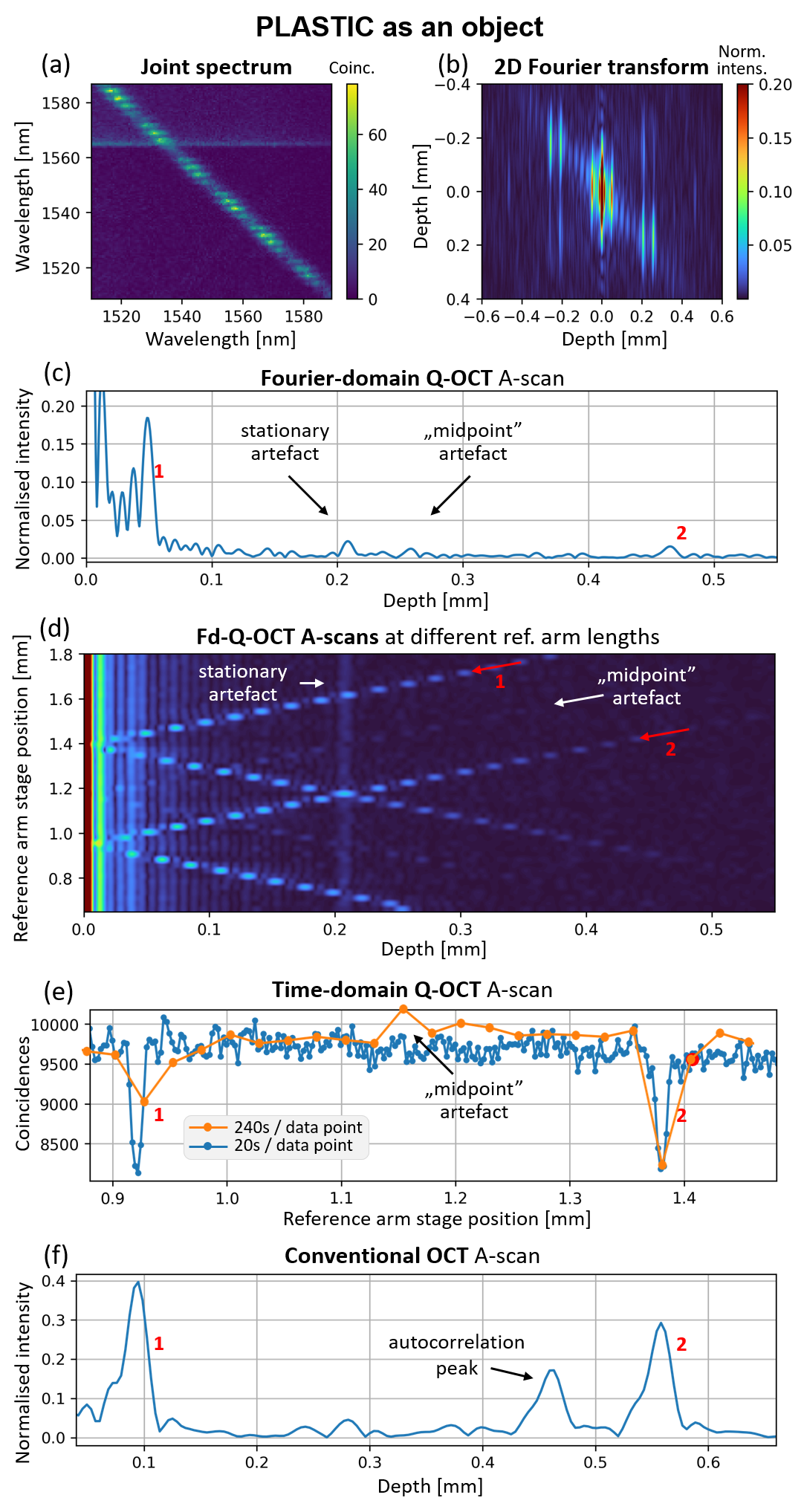
Figure 6: Measurement of the plastic sample. (a) Fibre-dispersion-corrected joint spectrum is (b) Fourier transformed and (c) the A-scan is extracted which shows two structural peaks, marked with 1 and 2. (d) A-scans for several consecutive reference arm stage positions further help distinguish the structural peaks (red) from artefacts (white). (e) An artefact is seen in the long-acquisition time-domain A-scan (orange), but is gone for short-acquisition time-domain A-scan (blue) due to noise. (f) Conventional OCT A-scan shows the structure of the object with a lower resolution and with an autocorrelation peak.

A piece of plastic, which is 260 $\mu$m thick, was used as an object and the joint spectrum was acquired for 4 minutes at the reference arm length being 45 $\mu$m bigger than the object arm length (the back-surface of the plastic serving in this case as the object arm’s end). The reference stage position at which the joint spectrum was measured is marked with a red dot in the time-domain signal in Fig. 6e). The A-scan is extracted (Fig. 6c) from the 2D Fourier transform (Fig. 6b) of the fibre-dispersion-corrected joint spectrum (Fig. 6a) and shows two peaks corresponding to the front and back surface of the plastic (marked with 1 and 2). Due to the small imaging range, the back-surface peak height is very small.

One can observe two artefacts, just as in the case of the glass. The presence of these artefacts is confirmed when the Fourier-domain A-scans extracted from joint spectra, acquired - 4 minutes each - for a range of reference arm stage positions are plotted together (Fig. 6d). Because the change of the reference arm stage results in the change in the position of the plastic structure in the A-scan, one observes two very bright elements approaching the 0 mm depth, marked with 1 and 2. There is an artefact halfway between the structural peaks ("midpoint" artefact, white arrow) travelling together with the structural peaks, and an artefact whose position is fixed (stationary artefact). Due to Fourier transformation ambiguity, the peaks do not cross over to the negative-frequency part of the transform, as one would expect, but continue on the same side but in the other direction.

The "midpoint" and stationary artefacts are much smaller with respect to the structural peaks than the artefacts for the glass (Fig. 5c), because the plastic is thicker than the glass. This confirms the theoretical findings in Ref. Kolenderska and Szkulmowski (2021) where it was noted that artefact suppression is the better, the bigger the anti-diagonal width of the joint spectrum and the thicker the object. Since the joint spectrum’s anti-diagonal width is the same for all the imaged objects, the difference in the reduction of the artefact height can come from the object thickness.

The coincidences in each joint spectrum behind the A-scan series in Fig. 6d were summed to create a time-domain A-scan, plotted in Fig. 6e in orange. Because the reference arm stage step was quite large, 50 $\mu$m, the resulting time-domain signal is undersampled, but one can still see the dips corresponding to the plastic structure and the unsuppressed "midpoint" artefact which in this case is a peak, not a dip.

Next, the reference stage position was varied with a smaller step, 5 $\mu$m, and much shorter integration time per step, 20 seconds, and the total coincidences were counted to form a denser time-domain A-scan, presented in Fig. 6e in blue. Two dips, each corresponding to a different plastic surface, are clearly visible, with no artefact observed as it is buried in the noise due to a small integration time. With a total of 258 points, the acquisition time was over 1.5 hours.

The conventional OCT A-scan, in Fig. 6f, shows both peaks as well as an autocorrelation peak with the widths larger than those of the peaks and dips in Q-OCT signals. Again, the conventional OCT spectrum was acquired in less than a second.

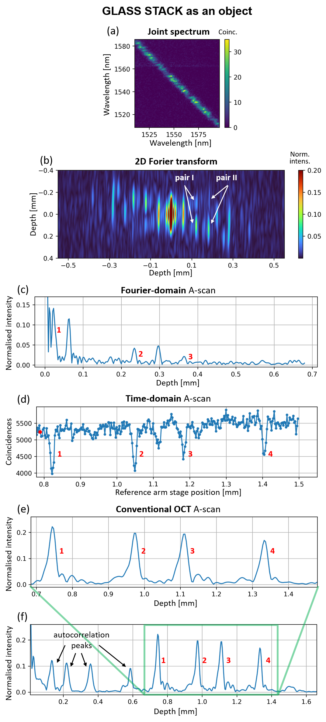
Figure 7: Measurement of a stack of thin glasses. (a) The joint spectrum was acquired. After fibre dispersion correction, (b) the joint spectrum was Fourier transformed and (c) the A-scan was extracted which shows three, out of the expected four, structural peaks - marked 1, 2 and 3, and two artefacts. (d) In the time-domain signal, all 4 structural elements are observed as dips, with one unsuppressed artefact dip. (e) Conventional OCT A-scan shows the structure of the object with a lower resolution and with autocorrelation peaks cluttering the front of (f) the A-scan.

Finally, a stack of two 100-$\mu$m-thick glasses was put as an object in the object arm and the joint spectrum was measured at the reference arm length being 35 $\mu$m shorter than the object arm length (the front surface of the stack marking the object arm end). Again, the reference stage position at which the joint spectrum was measured is marked with a red dot in the time-domain signal in Fig. 7d). The acquired joint spectrum is fibre dispersion corrected, Fig. 7a, and 2D Fourier transformed, Fig. 7b. Because the object comprises 4 interfaces - front and back surfaces of two pieces of glass - the 2D Fourier transform is cluttered with artefact elements. The A-scan extracted from it, Fig. 7c, is not free of artefacts, either. Also, due to the very limited imaging range, the fourth peak - corresponding to the back surface of the second piece of glass in the stack - is missing.

A careful analysis of the elements in the 2D Fourier transform leads to a conclusion that the artefact pairs become less symmetrical the deeper they are, compare pair I and II in Fig. 7b. This is also observed for the 2D Fourier transform representing the plastic (Fig. 6b) and is most probably due to the fibre dispersion whose influence increases with the depth.

In the time-domain A-scan, Fig. 7d, all four structural elements are clearly visible in the form of dips. Because the distance between interface 2 and interface 3 is small, the artefact corresponding to that pair is not suppressed. In the conventional OCT A-scan, Fig. 7e, one observes all four peaks as well. It should be noted that in this case, the reference stage position had to be chosen in a way such that the structural peaks do not overlap the autocorrelation peaks which clutter the front of the A-scan, see Fig. 7f.

The acquisition time of the single joint spectrum was again 4 minutes. The time-domain signal comprises 300 data points, each acquired in 30 seconds, resulting in a total acquisition time of over 2.5 hours. Again, the conventional OCT spectrum was acquired in less than a second.

Summary and discussion

We have provided an experimental demonstration of Fourier-domain Q-OCT, a modality theoretically proposed and analysed by us in 2020 Kolenderska et al. (2020b). The introduction of 5-kilometre-long fibre spools in the two detection Q-OCT channels allowed us to measure a two-dimensional joint spectrum of the interfering photon pairs for a variety of objects: a mirror, a thin piece of glass, a thick piece of plastic and a stack of two glasses. Interpolation algorithm was adopted from conventional OCT to correct for fibre dispersion distortions. Although this algorithm removed the chromatic dispersion effects induced by the fibre spools, this procedure did not affect the axial resolution, see Fig. 3, Fig. 5. It improved the quality of 2D Fourier transforms used to extract A-scans, facilitating identification of the artefacts. The coincidence post-selection data processing was introduced for precise and efficient A-scan extraction from the acquired joint spectra. As expected, the Fourier-domain Q-OCT A-scans showed the axial resolution much better than that obtained with the conventional OCT employing light of a similar bandwidth, see Fig. 4, and no even-order-dispersion-related degrading effects.

Our measurements validated the simulations from both Ref. Kolenderska et al. (2020b) and Ref. Kolenderska and Szkulmowski (2021): the 2D Fourier transforms of the joint spectra gave the expected insight into the limitations of the Q-OCT technique. The axial resolution depended on the diagonal width of the joint spectrum whereas its anti-diagonal width affected the artefact removal capabilities. As observed in the A-scans for the thin glass, Fig. 5e, and a thicker plastic,Fig. 6c, the anti-diagonal width allows a substantial reduction of the artefact peaks for the thicker plastic, but is not enough to affect the artefacts for the thinner glass. When corresponding 2D Fourier transforms are inspected, one sees that the artefact elements in there are very close to each other in the thin glass case, overlapping each other and consequently, producing non-zero values at the main diagonal. A remedy in this situation would be to reduce the anti-diagonal width of the artefact elements by employing a photon pair source whose antidiagonal joint-spectral width is larger.

It was also confirmed that Fourier-domain Q-OCT produces two artefact peaks per interface pair, one at the midpoint between the interfaces and one at the position equal to half the distance between the interfaces, as compared to one, "midpoint" artefact element in time-domain Q-OCT. A further comparison with the time-domain Q-OCT signal showed that the artefacts are equally suppressed for both modalities. This means that if one observes no artefacts in the time-domain signal, the Fourier-domain one will be artefact-free as well, and vice versa. The advantage of the Fourier-domain approach in this respect lies in the potential presented by the joint spectrum which gives unique access to the behaviour of the artefacts. As shown in Maliszewski and Kolenderska (2021); Maliszewski et al. (2022), when the joint spectrum is processed in a proper way and used as an input to a neural network, the artefacts could be easily identified and completely removed, a feature impossible with the time-domain signal. Also, Fourier-domain Q-OCT achieves better sensitivity than its time-domain counterpart. As shown on the example of the plastic, Fig. 6, Fourier-domain Q-OCT was able to capture a nearly-suppressed artefact after a 4-minute acquisition, whereas the time-domain signal - acquired for 1.5 hrs - could not as this artefact remained buried in the noise. Although in this particular case the artefact absence is a very welcomed outcome, one could imagine a scenario where the low-intensity peak which is not present is a structural element, rather than an artefact.

	Mirror	Thin glass	Thick plastic	Glass stack
Fourier-domain Q-OCT	10 s	3 min	4 min	4 min
Time-domain Q-OCT	2 min	30 min	1.5 hrs	2.5 hrs
Conventional OCT	< 1 s	< 1 s	< 1 s	< 1 s

Table 1: Total acquisition times for different OCT modalities presented in this article.

Fourier-domain Q-OCT is also very competitive with regards to the signal acquisition time. The summary of the total acquisition times for all objects imaged with the Fourier-domain Q-OCT is presented in Table 1, with the corresponding acquisition times for time-domain Q-OCT and conventional OCT included for reference. The Fourier-domain approach outperformed the time-domain approach: the more extended the imaged object is, the bigger the difference in the acquisition time. This is due to the fact that bulkier objects require a longer axial scan of the reference arm stage, resulting in the need to acquire more data points. In the case of a Fourier-domain signal, only a single joint spectrum is required. Although the acquisition times of Fd-Q-OCT are superior to the ones in time-domain Q-OCT, they are nowhere near the times achieved in conventional OCT, even when conventional OCT is performed with non-OCT-specific equipment, such as Optical Spectrum Analyser as is the case here.

As is generally the case in all Fourier-domain approaches, the imaging depth of Fourier-domain Q-OCT is restricted by the spectral resolution of the detection. The 5-kilometre-long fibre spools allow only 0.33 mm depth to be visualised, Fig. 4, resulting in barely visualising the back surface of the 260-$\mu$m-thick plastic (Fig. 6) and failure to visualise the bottom-most surface in the glass stack (Fig. 7). Longer fibre spools would increase the spectral resolution and extend the imaging depth, but at the same time, they would naturally attenuate the light more and consequently, require longer acquisition times.

There are also technical aspects to consider related to setting up and operating a Q-OCT system. Because the intensity of the quantum light is extremely low, one uses the classical laser light source to built and optimise the experimental system, ending up building a traditional OCT system either way. Similarly, due to long acquisition times, Q-OCT cannot be performed in real time. Because of that, the optimum position of the object in the object arm is found by switching to the classical light and maximising the intensity of light reflected from it. Consequently, conventional OCT remains to be an indispensible reference when performing the Q-OCT experiment.

There are several aspects of Fourier-domain Q-OCT which still need to be tackled. As shown here, the fibre dispersion correction did not make much impact on the imaging parameters, Fig. 4a,b, nor the quality of the A-scans, Fig. 5. This surprising result necessitates a thorough analysis based in both simulations and additional measurements, as an open question remains: is this lack of difference inherent or was the amount of fibre dispersion not sufficient to substantially deteriorate the signal? Such a study would certainly facilitate understanding of the behaviour of the 2D Fourier transform elements, including the depth-dependent asymetricity of the artefacts, compare Fig. 6b and Fig. 7b.

Another aspect worth exploring is further speeding up the measurement. What data acquisition parallelisation schemes could be employed to reduce the current record of 4 minutes for non-mirror objects (reported in this article)? Is there a scheme that will allow the world’s first fully non-invasive Q-OCT imaging of biological specimens? Or should we rather expect to achieve this when sufficient progress has been made in quantum light generation and detection?

Contributions

SMK and PK conceived the idea, SK and FCVdB carried out the measurements. All authors reviewed the manuscript.

Ethics declarations

Competing interests. The authors declare no competing interests.

References

- Abouraddy et al. (2002) A. F. Abouraddy, M. B. Nasr, B. E. Saleh, A. V. Sergienko, and M. C. Teich, Physical Review A 65, 053817 (2002).
- Nasr et al. (2003) M. B. Nasr, B. E. Saleh, A. V. Sergienko, and M. C. Teich, Physical review letters 91, 083601 (2003).
- Kolenderska et al. (2020a) S. M. Kolenderska, F. Vanholsbeeck, and P. Kolenderski, Optics Letters 45, 3443 (2020a).
- Hong et al. (1987) C.-K. Hong, Z.-Y. Ou, and L. Mandel, Physical review letters 59, 2044 (1987).
- Hayama et al. (2022) K. Hayama, B. Cao, R. Okamoto, S. Suezawa, M. Okano, and S. Takeuchi, Optics Letters 47, 4949 (2022).
- Yepiz-Graciano et al. (2022) P. Yepiz-Graciano, Z. Ibarra-Borja, R. Ramírez Alarcón, G. Gutiérrez-Torres, H. Cruz-Ramírez, D. Lopez-Mago, and A. B. U’Ren, Physical Review Applied 18, 034060 (2022).
- Sukharenko et al. (2021) V. Sukharenko, S. Bikorimana, and R. Dorsinville, Optics Letters 46, 2799 (2021).
- Ibarra-Borja et al. (2019) Z. Ibarra-Borja, C. Sevilla-Gutiérrez, R. Ramírez-Alarcón, H. Cruz-Ramírez, and A. B. U’Ren, Photonics Research 8, 51 (2019).
- Okano et al. (2015) M. Okano, H. H. Lim, R. Okamoto, N. Nishizawa, S. Kurimura, and S. Takeuchi, Scientific reports 5, 18042 (2015).
- Lopez-Mago and Novotny (2012) D. Lopez-Mago and L. Novotny, in Frontiers in Optics (Optica Publishing Group, 2012) pp. FTh4E–3.
- Nasr et al. (2009) M. B. Nasr, D. P. Goode, N. Nguyen, G. Rong, L. Yang, B. M. Reinhard, B. E. Saleh, and M. C. Teich, Optics Communications 282, 1154 (2009).
- Nasr et al. (2004) M. B. Nasr, B. E. Saleh, A. V. Sergienko, and M. C. Teich, Optics express 12, 1353 (2004).
- Yepiz-Graciano et al. (2020) P. Yepiz-Graciano, A. M. A. Martínez, D. Lopez-Mago, H. Cruz-Ramirez, and A. B. U’Ren, Photonics Research 8, 1023 (2020).
- Graciano et al. (2019) P. Y. Graciano, A. M. A. Martínez, D. Lopez-Mago, G. Castro-Olvera, M. Rosete-Aguilar, J. Garduño-Mejía, R. R. Alarcón, H. C. Ramírez, and A. B. U’Ren, Scientific Reports 9, 1 (2019).
- Teich et al. (2012) M. C. Teich, B. E. Saleh, F. N. Wong, and J. H. Shapiro, Quantum Information Processing 11, 903 (2012).
- Kolenderska et al. (2019) S. M. Kolenderska, F. Vanholsbeeck, and P. Kolenderski, in European Conference on Biomedical Optics (Optica Publishing Group, 2019) pp. 11078–30.
- Kolenderska et al. (2020b) S. M. Kolenderska, F. Vanholsbeeck, and P. Kolenderski, Optics Express 28, 29576 (2020b).
- Kolenderska and Szkulmowski (2021) S. M. Kolenderska and M. Szkulmowski, Scientific reports 11, 18585 (2021).
- Wang and Ding (2008) K. Wang and Z. Ding, Chinese Optics Letters 6, 902 (2008).
- Szkulmowski et al. (2016) M. Szkulmowski, S. Tamborski, and M. Wojtkowski, Biomedical optics express 7, 5042 (2016).
- Maliszewski and Kolenderska (2021) K. A. Maliszewski and S. M. Kolenderska, in Optical Coherence Tomography and Coherence Domain Optical Methods in Biomedicine XXV, Vol. 11630 (SPIE, 2021) pp. 19–27.
- Maliszewski et al. (2022) K. A. Maliszewski, S. M. Kolenderska, and V. Vetrova, in ICML 2022 2nd AI for Science Workshop (2022).
Acknowledgements
SMK acknowledges New Zealand Ministry of Business, Innovation and Employment (MBIE) Smart Ideas funding (E7943). The authors acknowledge the financial support from Horizon Europe, the European Union’s Framework Programme for Research and Innovation, SEQUOIA project, under Grant Agreement No. 101070062.