Equitable Auction Design: With and Without Distributions Equitable Auction Design: With and Without Distributions Wang, Koçyiğit, and Rujeerapaiboon Ruiqin Wang¹, Çağıl Koçyiğit², Napat Rujeerapaiboon^{1 1}Department of Industrial Systems Engineering and Management, National University of Singapore, Singapore
²Luxembourg Centre for Logistics and Supply Chain Management, University of Luxembourg, Luxembourg
ruiqin_wang@u.nus.edu, cagil.kocyigit@uni.lu, napat.rujeerapaiboon@nus.edu.sg

We study a mechanism design problem where a seller aims to allocate a good to multiple bidders, each with a private value. The seller supports or favors a specific group, referred to as the minority group. Specifically, the seller requires that allocations to the minority group are at least a predetermined fraction (equity level) of those made to the rest of the bidders. Such constraints arise in various settings, including government procurement and corporate supply chain policies that prioritize small businesses, environmentally responsible suppliers, or enterprises owned by historically disadvantaged individuals. We analyze two variants of this problem: stochastic mechanism design, which assumes bidders’ values follow a known distribution and seeks to maximize expected revenue, and regret-based mechanism design, which makes no distributional assumptions and aims to minimize the worst-case regret. We characterize a closed-form optimal stochastic mechanism and propose a closed-form regret-based mechanism, and establish that the ex-post regret under the latter is at most a constant multiple (dependent on the equity level) of the optimal worst-case regret. We further quantify that this approximation constant is at most 1.31 across different equity levels. Both mechanisms can be interpreted as set-asides, a common policy tool that reserves a fraction of goods for minority groups. Furthermore, numerical results demonstrate that the stochastic mechanism performs well when the bidders’ value distribution is accurately estimated, while the regret-based mechanism exhibits greater robustness under estimation errors.

1 Introduction

Auctions are widely used in practice to sell a diverse range of items, including housing, financial instruments, and commodities. Key reasons for employing auctions include the limited availability of the goods being offered and limited knowledge of demand, which necessitate a strategic allocation mechanism to achieve objectives such as revenue maximization, welfare maximization or regret minimization. In addition to these objectives, fairness and equity in allocations are important considerations in certain contexts, particularly when the goal is to support or favor a specific group, referred to here as the minority group. In fact, governments, in both procurement and allocation contexts, often have objectives to favor certain groups such as small businesses or enterprises owned by historically disadvantaged individuals. For instance, in the “Executive Order on Further Advancing Racial Equity and Support for Underserved Communities Through the Federal Government,” issued by the former president of the United States, Joseph R. Biden, the importance of equitable procurement is emphasized. Section 7 of this order sets a government-wide goal for federal procurement dollars, aiming for 15 percent to be awarded to small businesses owned by socially and economically disadvantaged individuals by Fiscal Year 2025 (Federal Register 2023). Another example is corporate procurement policies, where firms may set targets to source from environmentally responsible suppliers, small businesses, or suppliers owned by historically disadvantaged individuals to promote sustainability, innovation, and competition.

Motivated by the importance of incorporating fairness and equity into allocation mechanisms, in this paper, we study a mechanism design problem with equity constraints. In this problem, a seller aims to sell a good to multiple bidders, each with a privately known willingness-to-pay (value) for the good. The seller seeks to allocate a certain proportion of the good to the minority group, introducing equity constraints on allocation decisions. We formulate these equity constraints to ensure that they hold ex-post, i.e., after the bids have been revealed. We consider two variants of this mechanism design problem, each with a different objective: stochastic mechanism design, which assumes that the bidders’ values are random variables following a known distribution and aims to maximize the expected revenue, and regret-based mechanism design, which makes no assumptions about the distribution of the bidders’ values and aims to minimize the maximum regret in view of all possible bidders’ values, where regret is defined as the difference between the highest revenue achievable in hindsight and the revenue generated by a mechanism. While the first problem is relevant in scenarios involving large amounts of data or information, accurately estimating the distribution of bidders’ values can be challenging in many real-world settings. For instance, government auctions occur infrequently, resulting in limited available data. In such cases, the second problem becomes more practically relevant, as it does not rely on knowledge of the bidders’ value distributions.

The contributions of this paper are summarized as follows:

• For the stochastic mechanism design problem, we characterize the optimal mechanism in closed form for any equity level desired under a standard assumption on the bidders’ values—specifically, that they are mutually independent and their distributions are regular. The optimal mechanism can be interpreted as a set-aside, a method commonly used in practice where a certain fraction of the goods is reserved for allocation to the minority group; see, e.g., Athey et al. (2013). The fraction set aside for the minority group increases with and is uniquely determined by the equity level.

• Recognizing that in many practical situations, the seller is unlikely to know the underlying distribution of bidders’ values or estimate it accurately, we formulate the regret-based mechanism design problem with the objective of minimizing the worst-case regret. This approach neither relies on distributional assumptions nor requires knowledge of the bidders’ value distributions. We propose a mechanism and prove that its ex-post regret is at most a constant multiple of the optimal worst-case regret. This multiple depends on the level of equity targeted. We find (numerically) that this multiple is less than $1.31$ across all possible equity levels. We also show that the proposed mechanism is asymptotically optimal as the equity level decreases and increases. Similar to the optimal stochastic mechanism, there is also a set-aside implementation corresponding to this regret-based mechanism.

• We compare the two proposed mechanisms with additional benchmarks inspired by the literature, which can only be computed numerically, in a stress test experiment. Specifically, we derive the optimal stochastic mechanism based on the in-sample distribution and the regret-based mechanism, then assess the distributions of the revenues and regrets they generate under the out-of-sample distribution. Our results suggest that the optimal stochastic mechanism should be preferred when the two distributions are similar, while the regret-based mechanism performs better in other cases.

Consequently, we provide a closed-form, easy-to-implement mechanism with a provable performance guarantee, regardless of whether the distributional information of the bidders’ values is trustworthy.

Related Literature. Our work contributes to the mechanism design literature on fair allocations. The majority of this literature focuses on the fair division of resources without monetary transfers and studies various notions of fairness including envy-freeness, where agents prefer their own allocations over any allocation given to other agents (see, e.g., Barman et al. (2018)). Research on fair allocations in the context of auction design, particularly with consideration of group fairness (i.e., favoring a minority group), remains relatively limited. The closest works to ours in this line of research are Pai and Vohra (2012) and Fallah et al. (2024).

Pai and Vohra (2012) consider the mechanism design problem of a seller offering a single item to multiple buyers, subject to an equity constraint that requires buyers from a target group to win the item with an ex-ante probability of at least a given threshold, while maximizing efficiency. Fallah et al. (2024) study a similar problem in a dynamic setting where the seller interacts with two groups of buyers over multiple rounds. Their objective is to maximize discounted revenue while ensuring an equity constraint that requires the discounted average of items allocated to a target group up to any particular period, combined with the expected discounted allocation in future rounds, to exceed a given threshold. In both of these works, the underlying distribution of the buyers’ values is assumed to be known to the seller, and the equity constraints are enforced in expectation based on this distribution. In contrast, our paper formulates the equity constraints to hold ex-post, i.e., after the bids are revealed. Thus, while our notion of equity is similar in spirit to those studied in Pai and Vohra (2012) and Fallah et al. (2024), it does not rely on distributional assumptions or information and is guaranteed to hold irrespective of the underlying distribution. Additionally, we study the regret-based mechanism design problem, which does not require knowledge of the bidders’ value distributions, even in the objective. We therefore adopt a robust approach compared to these papers, both in terms of the objective (in the case of regret-based mechanism design) and the equity requirements (in both stochastic and regret-based mechanism design). Our robust approach not only reduces reliance on distributional knowledge but also simplifies the theoretical analysis, enabling us to characterize (approximately) optimal mechanisms in closed form.

Furthermore, our work contributes to the (distributionally) robust mechanism design literature (see, e.g., Anunrojwong et al. (2023), Chen et al. (2024), Wang (2024), Giannakopoulos et al. (2023), Rujeerapaiboon et al. (2023), Koçyiğit et al. (2024) and references therein), which assumes that only limited or no information about the bidders’ value distributions is available and evaluates mechanisms based on their performance under the most adverse distribution consistent with the available information. To the best of our knowledge, we are the first to study the robust auction design setting with equity constraints.

In addition, our work is related to other fair resource allocation problems, such as policy design for resource allocation based on contextual information (see, e.g., Jo et al. (2023), Tang et al. (2023), Freund et al. (2023), Bansak and Paulson (2024) and references therein). In particular, the equity notion we study in our paper resembles the concepts of minority prioritization and statistical parity (a.k.a., group fairness) in allocations, which should either be similar across different groups or favor minority groups, as studied in the respective literature.

Organization. The remainder of the paper is structured as follows. Section 2 introduces the problem formulations and preliminaries. Sections 3 and 4 study the stochastic and regret-based mechanism design problems, respectively. Section 5 presents the numerical experiments. Omitted proofs can be found in Appendix A, and additional experimental results are provided in Appendix B.

Notation. For any vector $\bm{v}\in\mathbb{R}^{I}$, we use $v_{i}$ to denote its $i^{\text{th}}$ component and $\bm{v}_{-i}$ to represent the subvector of $\bm{v}$ obtained by excluding $v_{i}$. Random vectors are indicated with a tilde (e.g., $\tilde{\bm{v}}$), while their realizations are denoted by the same symbols without the tilde (e.g., $\bm{v}$). The collection of all bounded Borel-measurable functions from a Borel set $\mathcal{A}$ to another Borel set $\mathcal{C}$ is denoted by $\mathcal{L}(\mathcal{A},\mathcal{C})$. Finally, $\log(\cdot)$ denotes the natural logarithm, and $\mathbb{I}_{\mathcal{E}}$ is the indicator function of the event $\mathcal{E}$.

2 Problem Formulation

We consider the auction design problem of a seller who wishes to sell a single good to $I\geq 2$ bidders. Let $\mathcal{I}=\{1,\dots,I\}$ represent the set of bidders. The bidders are categorized into two groups: minority and majority. Minority bidders, referring to a target group such as historically disadvantaged groups, may outnumber majority bidders. These classifications may be based on protected and observable features such as race, sex, age, etc. We use $\mathcal{I}^{\text{min}}=\{1,\dots,I^{\text{min}}\}$ and $\mathcal{I}^{\text{maj}}=\{I^{\text{min}}+1,\dots,I^{\text{min}}+I^{\text{maj}}\}$ to represent the sets of minority and majority bidders, respectively. The overall set $\mathcal{I}$ of bidders can be expressed as $\mathcal{I}=\mathcal{I}^{\text{min}}\cup\mathcal{I}^{\text{maj}}$. Each bidder $i\in\mathcal{I}$ assigns a value $v_{i}\in\mathcal{V}=[0,1]$ to the good, which is unknown to the seller and other bidders. We let $\bm{v}=(v_{1},\dots,v_{I})$ be the vector of all bidders’ values and denote by $\mathcal{V}^{I}=[0,1]^{I}$ the set of all bidders’ potential values.

By invoking the Revelation Principle, we focus on truthful direct mechanisms under which bidders choose to bid their true values (Myerson 1981). Formally, we define an auction as a mechanism $(\bm{q},\bm{m})$, comprising an allocation rule $\bm{q}\in\mathcal{L}(\mathcal{V}^{I},[0,1]^{I})$ and a payment rule $\bm{m}\in\mathcal{L}(\mathcal{V}^{I},\mathbb{R}^{I})$, that satisfies the following incentive compatibility (IC), individual rationality (IR) and allocation feasibility (AF) constraints.

$$q_{i}(v_{i},\bm{v}_{-i})v_{i}-m_{i}(v_{i},\bm{v}_{-i})\geq q_{i}(w_{i},\bm{v}_{-i})v_{i}-m_{i}(w_{i},\bm{v}_{-i})\;\;\;\forall i\in\mathcal{I},\forall\bm{v}\in\mathcal{V}^{I},\forall w_{i}\in\mathcal{V}$$ (IC)

$$q_{i}(v_{i},\bm{v}_{-i})v_{i}-m_{i}(v_{i},\bm{v}_{-i})\geq 0\;\;\;\forall i\in\mathcal{I},\forall\bm{v}\in\mathcal{V}^{I}$$ (IR)

$$\sum_{i\in\mathcal{I}}q_{i}(\bm{v})\leq 1\;\;\;\forall\bm{v}\in\mathcal{V}^{I}$$ (AF)

Given that the bidders report their values as $\bm{v}\in\mathcal{V}^{I}$, $q_{i}(\bm{v})$ represents the probability of allocating good to bidder $i\in\mathcal{I}$, and $m_{i}(\bm{v})$ represents the payment made by the same bidder. The incentive compatibility (IC) constraint ensures that every bidder has no incentive to misreport their value, the individual rationality (IR) constraint guarantees that every bidder’s utility cannot be negative when bidding truthfully, and the allocation feasibility (AF) constraint assures that the sum of allocation probabilities does not exceed $1$.

We will require that the allocation rule $\bm{q}$ satisfies the following equity (Eq) constraint, where $\gamma\geq 0$ quantifies the level of equity.

$$\sum_{i\in\mathcal{I}^{\text{min}}}q_{i}(\bm{v})\geq\gamma\sum_{i\in\mathcal{I}^{\text{maj}}}q_{i}(\bm{v})\;\;\;\forall\bm{v}\in\mathcal{V}^{I}$$ (Eq)

This constraint ensures that the probability of allocating the good to the minority group is at least as high as $\gamma$ times the one for the majority group, thereby ensuring equitable opportunities for the minority group. This principle is inspired by the approach of minority prioritization and statistical parity in allocations, which are employed, for example, in policy design for resource allocation based on contextual information (Tang et al. 2023, Jo et al. 2023).

Remark 2.1

In his “Executive Order on Further Advancing Racial Equity and Support for Undeserved Communities Through The Federal Government,” the former president of the United States, Joseph R. Biden, emphasizes the importance of equitable procurement. Section 7 of this order sets a government-wide goal for federal procurement dollars, aiming for 15 percent to be awarded to small businesses owned by socially and economically disadvantaged individuals in Fiscal Year 2025. Our formulation of equity (Eq) can articulate targets of this nature. In fact, consider the alternative equity constraint

$$\sum_{i\in\mathcal{I}^{\text{min}}}q_{i}(\bm{v})\geq\delta\sum_{i\in\mathcal{I}}q_{i}(\bm{v}),$$

where $\delta\in(0,1)$. This constraint requires that $\delta$ proportion of allocations be directed to bidders from the minority group. Note that this constraint can be written in the form of (Eq) as follows:

$$\sum_{i\in\mathcal{I}^{\text{min}}}q_{i}(\bm{v})\geq\delta\sum_{i\in\operatorname{\mathcal{I}^{\text{maj}}}}q_{i}(\bm{v})+\delta\sum_{i\in\operatorname{\mathcal{I}^{\text{min}}}}q_{i}(\bm{v})\iff\sum_{i\in\mathcal{I}^{\text{min}}}q_{i}(\bm{v})\geq\frac{\delta}{1-\delta}\sum_{i\in\operatorname{\mathcal{I}^{\text{maj}}}}q_{i}(\bm{v}).$$

$\Box$

In the following, we denote by $\mathcal{M}$ the set of mechanisms that satisfy (IC), (IR), (AF) and (Eq):

$$\mathcal{M}=\left\{(\bm{q},\bm{m})\in\mathcal{L}(\mathcal{V}^{I},[0,1]^{I})\times\mathcal{L}(\mathcal{V}^{I},\mathbb{R}^{I})\;\left|\;\eqref{eq:IC},\,\eqref{eq:IR},\,\eqref{eq:AF},\,\eqref{eq:Eq}\right.\right\}.$$

In this paper, we study two mechanism design problems: stochastic mechanism design, which assumes that the bidders’ values are random variables following a known distribution and aims to maximize the expected revenue, and regret-based mechanism design, which makes no assumptions about the distribution of the bidders’ values and aims to minimize the maximum regret, in view of all possible bidders’ values. We next formally introduce these two mechanism design problems.

Stochastic Mechanism Design

For the first problem setting, we model each bidder $i$’s value as a continuous random variable $\tilde{v}_{i}$ governed by a cumulative distribution function $\mathbb{F}_{i}$ with support $\mathcal{V}$. The joint cumulative distribution function of the bidders’ values is denoted by $\mathbb{F}$. We assume that $\mathbb{F}$ is known to the seller.

We formulate the stochastic mechanism design problem with the objective of maximizing the expected revenue as follows.

$$\max_{(\bm{q},\bm{m})\in\mathcal{M}} \mathbb{E}_{\mathbb{F}}\left[\sum_{i\in\mathcal{I}}m_{i}(\tilde{\bm{v}})\right]$$ (S-MDP)

We will characterize an optimal mechanism for problem (S-MDP) in Section 3. However, in certain practical scenarios, it may be unrealistic to assume that the seller knows the distribution $\mathbb{F}$. In such scenarios, it is not possible to characterize and implement the optimal mechanism that solves (S-MDP). This is the main motivation for employing a distribution-free approach and studying the regret-based mechanism design problem.

Regret-Based Mechanism Design

For the second problem setting, we do not make any distributional assumptions about the bidders’ values. The seller’s objective is to minimize the worst-case (maximum) regret across all possible realizations of the bidders’ values. The regret of a mechanism is defined as the difference between the revenue that could have been achieved with full knowledge of the bidders’ values and the actual revenue generated by the mechanism. If the seller knew the bidders’ true values $\bm{v}$, they could allocate the good to the highest bidder with probability $\frac{1}{1+\gamma}$ and to the highest bidder among the minority group with probability $\frac{\gamma}{1+\gamma}$. Each of these bidders would then be charged the product of their allocation probability and their true value. This allocation ensures that the equity constraint (Eq) is satisfied while also generating the highest possible revenue for the seller. The revenue generated by this allocation is given by

$$\frac{1}{1+\gamma}\max_{i\in\mathcal{I}}v_{i}+\frac{\gamma}{1+\gamma}\max_{i\in\mathcal{I}^{\text{min}}}v_{i},$$ (1)

which serves as a benchmark for what can be achieved with complete knowledge of the bidders’ values. Note that if the highest bidder among the minority group is also the highest bidder overall, the good is allocated to this bidder with probability one.

Noting that the worst-case regret is defined as the maximum regret over all possible bidders’ values in $\mathcal{V}^{I}$, we can now formulate the regret-based mechanism design problem with the objective of minimizing the worst-case regret as follows.

$$\min_{(\bm{q},\bm{m})\in\mathcal{M}}\;\max_{\bm{v}\in\mathcal{V}^{I}} \frac{1}{1+\gamma}\max_{i\in\mathcal{I}}v_{i}+\frac{\gamma}{1+\gamma}\max_{i\in\mathcal{I}^{\text{min}}}v_{i}-\sum_{i\in\mathcal{I}}m_{i}(\bm{v})$$ (R-MDP)

In Section 4, we will characterize a feasible mechanism that achieves a constant-factor approximation guarantee for problem (R-MDP).

Preliminaries

We close this section with some preliminaries that will be used in the following sections. The next lemma presents a well-known result available from the literature. Specifically, this lemma prescribes necessary and sufficient conditions for (IC) to hold.

Lemma 2.2 (See, e.g., Krishna (2009))

A mechanism $(\bm{q},\bm{m})$ satisfies (IC) if and only if, for all $i\in\mathcal{I}$,

• allocation rule $q_{i}$ is non-decreasing in bidder $i$’s value, i.e., $q_{i}(v_{i},\bm{v}_{-i})\geq q_{i}(w_{i},\bm{v}_{-i})$ for all $\bm{v}\in\mathcal{V}^{I}$ and $w_{i}\in\mathcal{V}:v_{i}\geq w_{i}$,

• payment rule $m_{i}$ satisfies $m_{i}(\bm{v})=q_{i}(\bm{v})v_{i}-\int_{0}^{{v}_{i}}q_{i}(x,\bm{v}_{-i})\text{d}x+m_{i}(0,\bm{v}_{-i})$ for all $\bm{v}\in\mathcal{V}^{I}$.

From (IR), it holds that $m_{i}(0,\bm{v}_{-i})\leq 0$ for all $i\in\mathcal{I}$, and at optimality of (S-MDP) and (R-MDP), it must hold that $m_{i}(0,\bm{v}_{-i})=0$ because the payments $m_{i}(\bm{v})$ are increasing in $m_{i}(0,\bm{v}_{-i})$.

3 Stochastic Mechanism Design

In this section, we characterize the optimal mechanism $(\bm{q}^{\star},\bm{m}^{\star})$ for problem (S-MDP). This characterization relies on the following assumption on the distribution of the bidders’ values, which we assume to hold throughout this section. [Independence & Regularity] Bidders’ values $\tilde{v}_{i}$ are mutually independent under $\mathbb{F}$. Furthermore, distribution $\mathbb{F}$ is regular, i.e., for all $i\in\mathcal{I}$, the marginal density $f_{i}$ of $\tilde{v}_{i}$ exists and is strictly positive on $\mathcal{V}$, and the virtual value function defined as

$$\psi_{i}(v_{i})=v_{i}-\frac{1-\mathbb{F}_{i}(v_{i})}{f_{i}(v_{i})}$$

is non-decreasing in $v_{i}$ on $\mathcal{V}$. Independence and regularity are standard assumptions and widely used in mechanism design literature. The class of regular distributions is very large and contains, for example, uniform, normal, logistic and exponential distributions and their truncations; see (Ewerhart 2013) for more details.

The next result reformulates problem (S-MDP) in terms of the virtual values.

Lemma 3.1 (See, e.g., Krishna (2009))

Problem (S-MDP) is equivalent to

$$\max \mathbb{E}_{\mathbb{F}}\left[\sum_{i\in\mathcal{I}}\psi_{i}(\tilde{v}_{i})q_{i}(\tilde{\bm{v}})\right]$$ (2)

  s.t. $$\bm{q}\in\mathcal{L}(\mathcal{V}^{I},[0,1]^{I}),\;\bm{m}\in\mathcal{L}(\mathcal{V}^{I},\mathbb{R}^{I})$$

$$q_{i}(v_{i},\bm{v}_{-i})\geq q_{i}(w_{i},\bm{v}_{-i})\;\;\;\forall i\in\mathcal{I},\forall\bm{v}\in\mathcal{V}^{I},\forall w_{i}\in\mathcal{V}:w_{i}\leq v_{i}$$

$$m_{i}(\bm{v})=q_{i}(\bm{v})v_{i}-\int_{0}^{{v}_{i}}q_{i}(x,\bm{v}_{-i})\text{d}x\;\;\;\forall i\in\mathcal{I},\forall\bm{v}\in\mathcal{V}^{I}$$

$$\eqref{eq:AF},\,\eqref{eq:Eq}.$$

We present the proof of Lemma 3.1 in Appendix A. The proof largely follows the arguments in (Krishna 2009, Chapter 5), with the addition of the equity constraint (Eq).

For all minority bidders $i\in\mathcal{I}^{\text{min}}$, we claim that the optimal allocation rule is defined as

$$q_{i}^{\star}(\bm{v})=\begin{cases}1&\text{if }i=\min\arg\max_{j\in\mathcal{I}}\psi_{j}(v_{j}),\,\psi_{i}(v_{i})\geq 0\\ \dfrac{\gamma}{1+\gamma}&\text{if }i=\min\arg\max_{j\in\mathcal{I}^{\text{min}}}\psi_{j}(v_{j}),\,\psi_{i}(v_{i})<\max_{j\in\mathcal{I}^{\text{maj}}}\psi_{j}(v_{j}),\\ &\quad\quad\quad\quad\quad\quad\quad\quad\quad\;\;\text{and }\max_{j\in\mathcal{I}^{\text{maj}}}\psi_{j}(v_{j})+\gamma\psi_{i}(v_{i})\geq 0,\\ 0&\text{otherwise,}\end{cases}$$

and for all majority bidders $i\in\mathcal{I}^{\text{maj}}$, it is defined as

$$q_{i}^{\star}(\bm{v})=\begin{cases}\dfrac{1}{1+\gamma}&\text{if }i=\min\arg\max_{j\in\mathcal{I}}\psi_{j}(v_{j}),\,\psi_{i}(v_{i})+\gamma\max_{j\in\mathcal{I}^{\text{min}}}\psi_{j}(v_{j})\geq 0\\ 0&\text{otherwise.}\end{cases}$$

In this paper, we use a lexicographic tie-breaker to break ties but this does not play a role in our analysis. By Lemma 2.2 (ii), for any $i\in\operatorname{\mathcal{I}}$, the optimal payment rule is given by

$$m_{i}^{\star}(\bm{v})=q^{\star}_{i}(\bm{v})v_{i}-\int_{0}^{{v}_{i}}q^{\star}_{i}(x,\bm{v}_{-i})\text{d}x.$$

We next establish the feasibility and the optimality of $(\bm{q}^{\star},\bm{m}^{\star})$.

Proposition 3.2

The mechanism $(\bm{q}^{\star},\bm{m}^{\star})$ belongs to $\mathcal{M}$ and is therefore feasible in (S-MDP).

Theorem 3.3

The mechanism $(\bm{q}^{\star},\bm{m}^{\star})$ is optimal in (S-MDP).

Proof 3.4

Proof of Theorem 3.3 Since (S-MDP) and (2) are equivalent by Lemma 3.1, it suffices to prove the optimality of $(\bm{q}^{\star},\bm{m}^{\star})$ in (2). To this end, first, we relax the monotonicity constraints of $q_{i}$ in $v_{i}$ in (2) and consider the relaxed problem

$$\max_{\bm{q}\in\mathcal{L}(\mathcal{V}^{I},[0,1]^{I})}\left\{\mathbb{E}_{\mathbb{F}}\left[\sum_{i\in\mathcal{I}}\psi_{i}(\tilde{v}_{i})q_{i}(\tilde{\bm{v}})\right]:\eqref{eq:AF},\,\eqref{eq:Eq}\right\}.$$ (3)

Note that the constraints related to the payment rule $\bm{m}$ in (2) can be omitted, allowing the problem to be solved only for the allocation rule $\bm{q}$ since $\bm{m}$ does not appear in any other constraints or the objective function. The optimal payment rule can be constructed after solving the problem by using the optimal allocation rule and setting $m_{i}(0,\bm{v}_{-i})=0$ for all $i\in\mathcal{I}$ and $\bm{v}_{-i}\in\mathcal{V}^{I-1}$ (see Lemma 2.2). Our strategy is to show that $\bm{q}^{\star}$ is optimal in (3). Given that $(\bm{q}^{\star},\bm{m}^{\star})$ is incentive compatible (see Proposition 3.2), it would then automatically hold that $\bm{q}^{\star}$ satisfies the omitted monotonicity constraints corresponding to (IC) (see Lemma 2.2), and hence $\bm{q}^{\star}$ would then be optimal not only in (3) but also in (2) and in (S-MDP).

To achieve this, we first observe that the objective and the constraints of (3) are decoupled over $\bm{v}\in\mathcal{V}^{I}$. Solving (3) is thus tantamount to solving the optimization problem

$$\max_{q(\bm{v})\in[0,1]^{I}}\left\{\sum_{i\in\mathcal{I}}\psi_{i}(v_{i})q_{i}(\bm{v}):\sum_{i\in\mathcal{I}}q_{i}(\bm{v})\leq 1,\sum_{i\in\mathcal{I}^{\text{min}}}q_{i}(\bm{v})\geq\gamma\sum_{i\in\mathcal{I}^{\text{maj}}}q_{i}(\bm{v})\right\},$$ (4)

which is parametrized in $\bm{v}\in\mathcal{V}^{I}$ and is a linear program consisting of $I$ decision variables. Introducing aggregate allocation variables for each group of bidders: $\tau^{\text{min}}(\bm{v})=\sum_{i\in\mathcal{I}^{\min}}q_{i}(\bm{v})$ and $\tau^{\text{maj}}(\bm{v})=\sum_{i\in\mathcal{I}^{\text{maj}}}q_{i}(\bm{v})$, we can relax (4) one step further as another parametrized linear program in $\bm{v}\in\mathcal{V}^{I}$:

$$\max_{\tau^{\text{min}}(\bm{v}),\tau^{\text{maj}}(\bm{v})\geq 0}\left\{\tau^{\text{min}}(\bm{v})\max_{i\in\mathcal{I}^{\text{min}}}\psi_{i}(v_{i})+\tau^{\text{maj}}(\bm{v})\max_{i\in\mathcal{I}^{\text{maj}}}\psi_{i}(v_{i}):\begin{array}[]{l}\tau^{\text{min}}(\bm{v})+\tau^{\text{maj}}(\bm{v})\leq 1\\ \tau^{\text{min}}(\bm{v})\geq\gamma\tau^{\text{maj}}(\bm{v})\end{array}\right\}$$ (5)

Problem (5) consists of only two variables and admits a vertex solution, that is, the optimal solution belongs to the set $\left\{(0,0),(1,0),(\gamma,1)/(1+\gamma)\right\}$ of vertices. When the highest minority virtual value $\max_{i\in\mathcal{I}^{\text{min}}}\psi_{i}(v_{i})$ surpasses the highest majority virtual value $\max_{i\in\mathcal{I}^{\text{min}}}\psi_{i}(v_{i})$ and is non-negative, $(1,0)$ is optimal. On the other hand, if the highest majority virtual value dominates and if $\max_{i\in\mathcal{I}^{\text{maj}}}\psi_{i}(v_{i})+\gamma\max_{i\in\mathcal{I}^{\text{min}}}\psi_{i}(v_{i})\geq 0$, then $(\gamma,1)/(1+\gamma)$ is optimal. Otherwise, the optimal solution of (5) is $(0,0)$. It turns out that (5) is in fact a tight relaxation because its optimal objective value can be attained by $\bm{q}^{\star}(\bm{v})$ in (4). As a result, for each $\bm{v}\in\mathcal{V}^{I}$, $\bm{q}^{\star}(\bm{v})$ is optimal in (4), and therefore $\bm{q}^{\star}$ itself is optimal in (3), (2), and (S-MDP). $\square$

Remark 3.5 (Set-aside Interpretation)

Set-asides are commonly used in the procurement and sales of resources to secure increased opportunities for target groups (Athey et al. 2013). These mechanisms set aside a fraction of the good(s) for the targeted (minority) group. The optimal mechanism $(\bm{q}^{\star},\bm{m}^{\star})$ incorporates a set-aside approach. Indeed, the optimal allocation rule $\bm{q}^{\star}$ can be equivalently expressed as:

$${q}^{\star}_{i}(\bm{v})=\frac{1}{1+\gamma}{q}_{i}^{\text{all}}(\bm{v})+\frac{\gamma}{1+\gamma}{q}_{i}^{\text{min}}(\bm{v})\;\;\;\forall i\in\mathcal{I},$$

where

$$q_{i}^{\text{all}}(\bm{v})=\begin{cases}1&\text{if }i=\min\arg\max_{j\in\mathcal{I}}\psi_{j}(v_{j}),\psi_{i}(v_{i})+\gamma\max_{j\in\operatorname{\mathcal{I}^{\text{min}}}}\psi_{j}(v_{j})\geq 0\\ 0&\text{otherwise,}\end{cases}$$

and

$$q_{i}^{\text{min}}(\bm{v})=\begin{cases}1&\text{if }i=\min\arg\max_{j\in\operatorname{\mathcal{I}^{\text{min}}}}\psi_{j}(v_{j}),\max_{j\in\operatorname{\mathcal{I}}}\psi_{j}(v_{j})+\gamma\psi_{i}(v_{i})\geq 0\\ 0&\text{otherwise.}\end{cases}$$

Note that $\bm{q}^{\text{min}}$ allocates exclusively to the minority group. Therefore, the optimal allocation $\bm{q}^{\star}$ reserves a fraction of goods, specifically $\frac{\gamma}{1+\gamma}$, for allocation to the minority group. The payment rule $\bm{m}^{\star}$ can similarly be expressed as $\frac{1}{1+\gamma}\bm{m}^{\text{all}}(\bm{v})+\frac{\gamma}{1+\gamma}\bm{m}^{\text{min}}(\bm{v})$, where $\bm{m}^{\text{all}}$ and $\bm{m}^{\text{min}}$ are defined according to Lemma 2.2(ii) as functions of $\bm{q}^{\text{all}}$ and $\bm{q}^{\text{min}}$, respectively. $\Box$

While the stochastically optimal mechanism adopts a set-aside interpretation—a method commonly used in practice—it could be challenging to compute and implement. The difficulty arises because the optimal mechanism heavily depends on the value distribution $\mathbb{F}$, which may not be known to the seller and is therefore subject to estimation errors. For this reason, in Section 4, we study regret-based mechanism design and propose a mechanism that provides a provable approximation guarantee for the optimal worst-case regret of problem (R-MDP). This mechanism and its performance guarantee do not rely on any distributional assumptions.

4 Regret-Based Mechanism Design

In this section, we propose a mechanism that is approximately optimal in (R-MDP). In particular, we demonstrate that this mechanism generates a regret that is at most a constant multiple of the optimal value of (R-MDP). We will establish this by deriving a lower bound on the optimal value of (R-MDP) and an upper bound on the ex-post regret of the proposed mechanism. For ease of exposition, from now on we denote by ${\text{REG}}_{(\bm{q},\bm{m})}(\bm{v})$ the regret of a mechanism $(\bm{q},\bm{m})$ that is incurred for a given value $\bm{v}\in\mathcal{V}^{I}$, which is defined as

$${\text{REG}}_{(\bm{q},\bm{m})}(\bm{v})= \frac{1}{1+\gamma}\max_{i\in\mathcal{I}}v_{i}+\frac{\gamma}{1+\gamma}\max_{i\in\mathcal{I}^{\text{min}}}v_{i}-\sum_{i\in\mathcal{I}}m_{i}(\bm{v}).$$

Thus, the objective of (R-MDP) can be expressed as $\max_{\bm{v}\in\mathcal{V}^{I}}{\text{REG}}_{(\bm{q},\bm{m})}(\bm{v})$.

First, we establish a lower bound on the optimal value of (R-MDP).

Theorem 4.1 (Lower Bound)

For any $(\bm{q},\bm{m})\in\mathcal{M}$, it holds that $\max_{\bm{v}\in\mathcal{V}^{I}}{\text{REG}}_{(\bm{q},\bm{m})}(\bm{v})\geq\frac{1}{e}$.

Proof 4.2

Proof of Theorem 4.1 We will prove the claim by showing that the optimal value of (R-MDP) for any number of bidders is bounded below by the optimal value of (R-MDP) with only a single minority bidder, and that the optimal value of the latter problem is $\frac{1}{e}$. To this end, consider bidder $1$ in the minority group and assume that the values of all other bidders are zero, i.e., $\bm{v}_{-1}=\bm{0}$. A lower bound on the optimal value of (R-MDP) arising from such $\bm{v}$ can be characterized as follows:

$$\min_{(\bm{q},\bm{m})\in\mathcal{M}}\max_{\bm{v}\in\mathcal{V}^{I}}{\text{REG}}_{(\bm{q},\bm{m})}(\bm{v})\geq \min_{(\bm{q},\bm{m})\in\mathcal{M}}\max_{v_{1}\in\mathcal{V}}{\text{REG}}_{(\bm{q},\bm{m})}(v_{1},\bm{0})\geq \min_{(\bm{q},\bm{m})\in\mathcal{M}}\max_{v_{1}\in\mathcal{V}}v_{1}-m_{1}({v}_{1},\bm{0}),$$

where the second inequality holds since $m_{i}(v_{i},\bm{0})\leq 0$ for all $i\in\mathcal{I}\setminus\{1\}$ because of (IR). The last minimax problem above is closely related to a version of (R-MDP) which involves a single (minority) bidder. Note that when there are no majority bidders, the equity requirement (Eq) is no longer enforced, and likewise (AF) becomes redundant. Let $\mathcal{M}^{\dagger}\subseteq\mathcal{L}(\mathcal{V},[0,1])\times\mathcal{L}(\mathcal{V},\mathbb{R})$ denote the feasible set of all mechanisms $(q^{\dagger},m^{\dagger})$ satisfying the following incentive compatibility and individual rationality constraints:

$$q^{\dagger}(v)v-m^{\dagger}(v)\geq q^{\dagger}(w)v-m^{\dagger}(w)\;\;\;\forall v,w\in\mathcal{V}\quad\text{and}\quad q^{\dagger}(v)v-m^{\dagger}(v)\geq 0\;\;\;\forall v\in\mathcal{V}.$$

It can be readily verified that, for any $(\bm{q},\bm{m})\in\mathcal{M}$, $(q_{1}(\cdot,\bm{0}),m_{1}(\cdot,\bm{0}))$ belongs to $\mathcal{M}^{\dagger}$. Hence,

$$\min_{(\bm{q},\bm{m})\in\mathcal{M}}\max_{v_{1}\in\mathcal{V}}v_{1}-m_{1}({v}_{1},\bm{0})\geq\min_{(q^{\dagger},m^{\dagger})\in\mathcal{M}^{\dagger}}\max_{v\in\mathcal{V}}v-m^{\dagger}(v)=\dfrac{1}{e},$$

where the equality holds thanks to known results for the optimal worst-case regret in the single-bidder case, as shown in Bergemann and Schlag (2008) and Koçyiğit et al. (2022). The claim thus follows. $\square$

Next, we propose a mechanism $(\bm{\hat{q}},\bm{\hat{m}})$, and then, in Theorem 4.4, we characterize an upper bound on its regret ${\text{REG}}_{(\bm{\hat{q}},\bm{\hat{m}})}(\bm{v})$ across all $\bm{v}\in\mathcal{V}^{I}$, which thereby also bounds the optimal value of (R-MDP). To define $(\bm{\hat{q}},\bm{\hat{m}})$, from now on, we denote by ${i^{\text{min}}(\bm{v})}$ (respectively, ${i^{\text{maj}}(\bm{v})}$) the bidder who has the largest value in the minority (respectively, majority) group. We again use the lexicographical rule to break ties when there are multiple such bidders, that is,

$${i^{\text{min}}(\bm{v})}=\min\arg\max_{i\in\mathcal{I}^{\text{min}}}v_{i}\quad\text{and}\quad{i^{\text{maj}}(\bm{v})}=\min\arg\max_{i\in\mathcal{I}^{\text{maj}}}v_{i}.$$

Then, we define the mechanism $(\bm{\hat{q}},\bm{\hat{m}})$ as follows. For all minority bidders $i\in\mathcal{I}^{\text{min}}$,

$${\hat{q}}_{i}(\bm{v})=\begin{cases}\dfrac{\gamma}{1+\gamma}\left(1+\log{\ell(\bm{v})}\right)^{+}&\text{ if }i={i^{\text{min}}(\bm{v})}\text{ and }v_{{i^{\text{maj}}(\bm{v})}}>v_{{i^{\text{min}}(\bm{v})}}\\ \left(1+\log v_{i}\right)^{+}&\text{ if }i={i^{\text{min}}(\bm{v})}\text{ and }v_{{i^{\text{maj}}(\bm{v})}}\leq v_{{i^{\text{min}}(\bm{v})}}\\ 0&\text{ otherwise,}\end{cases}$$

and, for all majority bidders $i\in\mathcal{I}^{\text{maj}}$,

$${\hat{q}}_{i}(\bm{v})=\begin{cases}\dfrac{1}{1+\gamma}\left(1+\log{\ell(\bm{v})}\right)^{+}&\text{ if }i={i^{\text{maj}}(\bm{v})}\text{ and }v_{{i^{\text{maj}}(\bm{v})}}>v_{{i^{\text{min}}(\bm{v})}}\\ 0&\text{ otherwise,}\end{cases}$$

where

$$\ell(\bm{v})=\frac{\gamma}{1+\gamma}v_{{i^{\text{min}}(\bm{v})}}+\frac{1}{1+\gamma}v_{{i^{\text{maj}}(\bm{v})}}.$$ (6)

Note that $\ell(\bm{v})$ matches the highest possible revenue (1) for the seller in hindsight whenever $v_{{i^{\text{maj}}(\bm{v})}}$ exceeds $v_{{i^{\text{min}}(\bm{v})}}$. Finally, we let

$${\hat{m}}_{i}(\bm{v})=v_{i}{\hat{q}}_{i}(\bm{v})-\int_{0}^{v_{i}}{\hat{q}}_{i}(x,\bm{v}_{-i}){\rm{d}}x\quad\forall i\in\mathcal{I}.$$

Under this mechanism, only the highest bidder from the minority group and the highest bidder from the majority group have a non-zero chance of being allocated the item. Specifically, if the highest minority bid exceeds the highest majority bid, the item cannot be allocated to any majority bidder. Conversely, if the highest bid comes from the majority group, the probability of allocating the item to the highest majority bidder is limited to $1/\gamma$ times the probability of allocating it to the highest minority bidder, ensuring fairness.

This mechanism is feasible in (R-MDP) as we formalize in the following proposition.

Proposition 4.3

The mechanism $(\bm{\hat{q}},\bm{\hat{m}})$ belongs to $\mathcal{M}$ and is therefore feasible in (R-MDP).

Next, we establish an upper bound on the ex-post regret of the feasible mechanism $(\bm{\hat{q}},\bm{\hat{m}})$.

Theorem 4.4 (Upper Bound)

The ex-post regret of the mechanism $(\hat{\bm{q}},\hat{\bm{m}})$ satisfies

$${\text{REG}}_{(\bm{\hat{q}},\bm{\hat{m}})}(\bm{v})\leq\left(\frac{1+\gamma u^{\star}}{1+\gamma}\right)\log\left(\frac{1+\gamma u^{\star}}{1+\gamma}\right)-u^{\star}\log u^{\star}-\beta^{\star}\log\beta^{\star}\quad\forall\bm{v}\in\mathcal{V}^{I},$$

where $\beta^{\star}=\max\left\{\frac{1}{1+\gamma},\frac{1}{e}\right\}$ and $u^{\star}\in\left[\frac{1}{e},1\right]$ is a unique root of

$$\frac{\gamma}{1+\gamma}\log\left(\frac{1+\gamma u}{1+\gamma}\right)-\log u-\frac{1}{1+\gamma}=0.$$

Proof 4.5

Proof of Theorem 4.4 For ease of exposition, we denote the upper bound on ${\text{REG}}_{(\bm{\hat{q}},\bm{\hat{m}})}(\bm{v})$ given in Theorem 4.4 by $\theta$. Note that $\theta$ depends on $\gamma,\beta^{\star}$ and $u^{\star}$, but it doesn’t depend on $\bm{v}$. Fixing an arbitrary $\bm{v}\in\mathcal{V}^{I}$, we will first prove that ${\text{REG}}_{(\bm{\hat{q}},\bm{\hat{m}})}(\bm{v})\leq\max\{\theta,\frac{1}{e}\}$ separately for two cases: Case 1 ($v_{{i^{\text{maj}}(\bm{v})}}>v_{{i^{\text{min}}(\bm{v})}}$) and Case 2 ($v_{{i^{\text{maj}}(\bm{v})}}\leq v_{{i^{\text{min}}(\bm{v})}}$). After proving the inequality for these two cases, we will demonstrate that $\theta\geq\frac{1}{e}$, which will conclude the proof.

Case 1 ($v_{{i^{\text{maj}}(\bm{v})}}>v_{{i^{\text{min}}(\bm{v})}}$): Recalling the definition of $\ell(\bm{v})$ in (6), we can write $\text{REG}_{(\bm{\hat{q}},\bm{\hat{m}})}(\bm{v})$ as

$$\text{REG}_{(\bm{\hat{q}},\bm{\hat{m}})}(\bm{v})=\ell(\bm{v})-\sum_{i\in\mathcal{I}^{\text{min}}}\hat{m}_{i}(\bm{v})-\sum_{i\in\mathcal{I}^{\text{maj}}}\hat{m}_{i}(\bm{v})=\ell(\bm{v})-\hat{m}_{i^{\text{min}}(\bm{v})}(\bm{v})-\hat{m}_{i^{\text{maj}}(\bm{v})}(\bm{v}),$$

where the second equality follows from the definition of $(\bm{\hat{q}},\bm{\hat{m}})$. That is, only the highest bidders from each group have a non-zero chance of being allocated the item and may be charged non-zero payments. By the definition of $\bm{\hat{m}}$, the regret above can be equivalently expressed as

$$\text{REG}_{(\bm{\hat{q}},\bm{\hat{m}})}(\bm{v})=\ell(\bm{v}) -v_{{i^{\text{min}}(\bm{v})}}{\hat{q}}_{{i^{\text{min}}(\bm{v})}}(\bm{v})+\int_{0}^{v_{{i^{\text{min}}(\bm{v})}}}{\hat{q}}_{{i^{\text{min}}(\bm{v})}}(x,\bm{v}_{-{{i^{\text{min}}(\bm{v})}}}){\rm{d}}x$$ (7)

$$-v_{{i^{\text{maj}}(\bm{v})}}{\hat{q}}_{{i^{\text{maj}}(\bm{v})}}(\bm{v})+\int_{0}^{v_{{i^{\text{maj}}(\bm{v})}}}{\hat{q}}_{{i^{\text{maj}}(\bm{v})}}(x,\bm{v}_{-{{i^{\text{maj}}(\bm{v})}}}){\rm{d}}x.$$

To bound $\text{REG}_{(\bm{\hat{q}},\bm{\hat{m}})}(\bm{v})$, we first study the two integrals on the right-hand side of (7) individually. For the first integral, we have

$$\int_{0}^{v_{{i^{\text{min}}(\bm{v})}}}{\hat{q}}_{{i^{\text{min}}(\bm{v})}}(x,\bm{v}_{-{{i^{\text{min}}(\bm{v})}}}){\rm{d}}x$$ (8)

$$= \int_{0}^{v_{{i^{\text{min}}(\bm{v})}}}\dfrac{\gamma}{1+\gamma}\left(1+\log(\dfrac{\gamma}{1+\gamma}x+\dfrac{1}{1+\gamma}v_{{i^{\text{maj}}(\bm{v})}})\right)^{+}\mathds{I}_{\{x\geq\max_{j\in\mathcal{I}^{\text{min}}\setminus\{i^{\text{min}}(\bm{v})\}}v_{j}\}}{\rm{d}}x$$

$$\leq \int_{0}^{v_{{i^{\text{min}}(\bm{v})}}}\dfrac{\gamma}{1+\gamma}\left(1+\log(\dfrac{\gamma}{1+\gamma}x+\dfrac{1}{1+\gamma}v_{{i^{\text{maj}}(\bm{v})}})\right)^{+}{\rm{d}}x$$

$$= \int_{0}^{\frac{\gamma}{1+\gamma}v_{{i^{\text{min}}(\bm{v})}}}\left(1+\log(y+\dfrac{1}{1+\gamma}v_{{i^{\text{maj}}(\bm{v})}})\right)^{+}{\rm{d}}y$$

$$= \int_{\frac{1}{1+\gamma}v_{{i^{\text{maj}}(\bm{v})}}}^{\frac{\gamma}{1+\gamma}v_{{i^{\text{min}}(\bm{v})}}+\frac{1}{1+\gamma}v_{{i^{\text{maj}}(\bm{v})}}}\left(1+\log z\right)^{+}{\rm{d}}z=\int_{\frac{1}{1+\gamma}v_{{i^{\text{maj}}(\bm{v})}}}^{\ell(\bm{v})}\left(1+\log z\right)^{+}{\rm{d}}z,$$

where the first equality follows from the definition of $\hat{q}_{i^{\text{min}}(\bm{v})}$, and the next two equalities follow from affine transformations $y=\frac{\gamma}{1+\gamma}x$ and $z=y+\frac{1}{1+\gamma}v_{{i^{\text{maj}(\bm{v})}}}$, respectively. Finally, the last equality follows from the definition of $\ell(\bm{v})$.

For the second integral on the right-hand side of (7), we have

$$\int_{0}^{v_{{i^{\text{maj}}(\bm{v})}}}{\hat{q}}_{{i^{\text{maj}}(\bm{v})}}(x,\bm{v}_{-{{i^{\text{maj}}(\bm{v})}}}){\rm{d}}x$$ (9)

$$= \int_{v_{{i^{\text{min}}(\bm{v})}}}^{v_{{i^{\text{maj}}(\bm{v})}}}\dfrac{1}{1+\gamma}\left(1+\log(\dfrac{\gamma}{1+\gamma}v_{{i^{\text{min}}(\bm{v})}}+\dfrac{1}{1+\gamma}x)\right)^{+}\mathds{I}_{\{x\geq\max_{j\in\mathcal{I}^{\text{maj}}\setminus\{i^{\text{maj}}(\bm{v})\}}v_{j}\}}{\rm{d}}x$$

$$\leq \int_{v_{{i^{\text{min}}(\bm{v})}}}^{v_{{i^{\text{maj}}(\bm{v})}}}\dfrac{1}{1+\gamma}\left(1+\log(\dfrac{\gamma}{1+\gamma}v_{{i^{\text{min}}(\bm{v})}}+\dfrac{1}{1+\gamma}x)\right)^{+}{\rm{d}}x$$

$$= \int_{\frac{1}{1+\gamma}v_{{i^{\text{min}}(\bm{v})}}}^{\frac{1}{1+\gamma}v_{{i^{\text{maj}}(\bm{v})}}}\left(1+\log(\dfrac{\gamma}{1+\gamma}v_{{i^{\text{min}}(\bm{v})}}+y)\right)^{+}{\rm{d}}y$$

$$= \int_{v_{{i^{\text{min}}(\bm{v})}}}^{\frac{1}{1+\gamma}v_{{i^{\text{maj}}(\bm{v})}}+\frac{\gamma}{1+\gamma}v_{{i^{\text{min}}(\bm{v})}}}\left(1+\log z\right)^{+}{\rm{d}}z=\int_{v_{{i^{\text{min}}(\bm{v})}}}^{\ell(\bm{v})}\left(1+\log z\right)^{+}{\rm{d}}z,$$

where, similarly to before, the first equality follows from the definition of $\hat{q}_{i^{\text{maj}}(\bm{v})}$ and the next two equalities follow from affine transformations $y=\frac{1}{1+\gamma}x$ and $z=\frac{\gamma}{1+\gamma}v_{{i^{\text{min}}(\bm{v})}}+y$, respectively. We thus bound the two integrals from above.

Next, we consider the term $v_{{i^{\text{min}}(\bm{v})}}{\hat{q}}_{{i^{\text{min}}(\bm{v})}}(\bm{v})+v_{{i^{\text{maj}}(\bm{v})}}{\hat{q}}_{{i^{\text{maj}}(\bm{v})}}(\bm{v})$, which also appears on the right-hand side of (7). This term can be expressed equivalently as

$$v_{{i^{\text{min}}(\bm{v})}}{\hat{q}}_{{i^{\text{min}}(\bm{v})}}(\bm{v})+v_{{i^{\text{maj}}(\bm{v})}}{\hat{q}}_{{i^{\text{maj}}(\bm{v})}}(\bm{v})$$ (10)

$$= \dfrac{\gamma}{1+\gamma}v_{{i^{\text{min}}(\bm{v})}}\left(1+\log{\ell(\bm{v})}\right)^{+}+\dfrac{1}{1+\gamma}v_{{i^{\text{maj}}(\bm{v})}}\left(1+\log{\ell(\bm{v})}\right)^{+}=\ell(\bm{v})\left(1+\log{\ell(\bm{v})}\right)^{+},$$

where the first equality follows from the definitions of ${\hat{q}}_{{i^{\text{min}}(\bm{v})}}$ and ${\hat{q}}_{{i^{\text{maj}}(\bm{v})}}$, and the second equality follows from the definition of $\ell(\bm{v})$.

Leveraging the algebraic insights from (8), (9) and (10), we can now bound the regret in (7) from above by $\overline{\text{REG}}_{(\bm{\hat{q}},\bm{\hat{m}})}(\bm{v})$ that is defined as

$$\overline{\text{REG}}_{(\bm{\hat{q}},\bm{\hat{m}})}(\bm{v})=\ell(\bm{v})-\ell(\bm{v})\left(1+\log{\ell(\bm{v})}\right)^{+}+\int_{\frac{1}{1+\gamma}v_{{i^{\text{maj}}(\bm{v})}}}^{\ell(\bm{v})}\left(1+\log z\right)^{+}{\rm{d}}z+\int_{v_{{i^{\text{min}}(\bm{v})}}}^{\ell(\bm{v})}\left(1+\log z\right)^{+}{\rm{d}}z.$$

If $\ell(\bm{v})<\frac{1}{e}$, then we have $\overline{\text{REG}}_{(\bm{\hat{q}},\bm{\hat{m}})}(\bm{v})\leq\ell(\bm{v})<\frac{1}{e}$.

For the case $\ell(\bm{v})\geq\frac{1}{e}$, we will first show that $\overline{\text{REG}}_{(\bm{\hat{q}},\bm{\hat{m}})}(\bm{v})$ increases as $v_{i^{\text{maj}}(\bm{v})}$ increases. We will then use this observation to argue that $\overline{\text{REG}}_{(\bm{\hat{q}},\bm{\hat{m}})}(\bm{v})$ is bounded above by $\overline{\text{REG}}_{(\bm{\hat{q}},\bm{\hat{m}})}(\bm{v}^{\prime})$, where $\bm{v}^{\prime}$ is the value profile obtained by increasing $v_{i^{\text{maj}}(\bm{v})}$ to $1$ (its maximum possible value) while keeping the values of the other bidders unchanged. Supposing $\ell(\bm{v})\geq\frac{1}{e}$, we have

$$\overline{\text{REG}}_{(\bm{\hat{q}},\bm{\hat{m}})}(\bm{v}) =-\ell(\bm{v})\log{\ell(\bm{v})}+\int_{\frac{1}{1+\gamma}v_{{i^{\text{maj}}(\bm{v})}}}^{\ell(\bm{v})}\left(1+\log z\right)^{+}{\rm{d}}z+\int_{v_{{i^{\text{min}}(\bm{v})}}}^{\ell(\bm{v})}\left(1+\log z\right)^{+}{\rm{d}}z$$

$$=-\ell(\bm{v})\log{\ell(\bm{v})}+\int_{\max\left\{\frac{1}{1+\gamma}v_{{i^{\text{maj}}(\bm{v})}},\frac{1}{e}\right\}}^{\ell(\bm{v})}\left(1+\log z\right){\rm{d}}z+\int_{\max\left\{v_{{i^{\text{min}}(\bm{v})}},\frac{1}{e}\right\}}^{\ell(\bm{v})}\left(1+\log z\right){\rm{d}}z$$

$$=\ell(\bm{v})\log\ell(\bm{v})-\alpha(\bm{v})\log\alpha(\bm{v})-\beta(\bm{v})\log\beta(\bm{v}),$$

where mappings $\alpha$ and $\beta$ are defined as

$$\alpha(\bm{v})=\max\left\{v_{{i^{\text{min}}(\bm{v})}},\frac{1}{e}\right\}\quad\text{and}\quad\beta(\bm{v})=\max\left\{\frac{1}{1+\gamma}v_{{i^{\text{maj}}(\bm{v})}},\frac{1}{e}\right\}.$$

If $\beta(\bm{v})=\frac{1}{e}$ while $\ell(\bm{v})\geq\frac{1}{e}$, $\ell(\bm{v})\log\ell(\bm{v})$ is increasing in $\ell(\bm{v})$ and particularly in $v_{i^{\text{maj}}(\bm{v})}$. As $\alpha(\bm{v})$ does not depend on $v_{i^{\text{maj}}(\bm{v})}$, $\overline{\text{REG}}_{(\bm{\hat{q}},\bm{\hat{m}})}(\bm{v})$ is also increasing in $v_{i^{\text{maj}}(\bm{v})}$. If $\beta(\bm{v})=\frac{1}{1+\gamma}v_{{i^{\text{maj}}(\bm{v})}}>\frac{1}{e}$, we have

$$\ell(\bm{v})\log\ell(\bm{v})-\beta(\bm{v})\log\beta(\bm{v})=\left(\beta(\bm{v})+\frac{\gamma}{1+\gamma}v_{i^{\text{min}}(\bm{v})}\right)\log\left(\beta(\bm{v})+\frac{\gamma}{1+\gamma}v_{i^{\text{min}}(\bm{v})}\right)-\beta(\bm{v})\log\beta(\bm{v}),$$

where the equality follows from the definition of $\ell(\bm{v})$. The above term increases as $\beta(\bm{v})$ increases (and consequently as $v_{i^{\text{maj}}(\bm{v})}$ increases) because

$$\derivative{\eta}\left((\eta+\delta)\log(\eta+\delta)-\eta\log\eta\right)=\log\left(1+\frac{\delta}{\eta}\right)>0\quad\forall\eta>0,\delta\geq 0.$$

Hence, regardless of the value of $\beta(\bm{v})$, we find that $\overline{\text{REG}}_{(\bm{\hat{q}},\bm{\hat{m}})}(\bm{v})$ always increases with $v_{i^{\text{maj}}(\bm{v})}$. We can thus conclude that

$$\overline{\text{REG}}_{(\bm{\hat{q}},\bm{\hat{m}})}(\bm{v}) \leq\overline{\text{REG}}_{(\bm{\hat{q}},\bm{\hat{m}})}(\bm{v}^{\prime})$$ (11)

$$=\left(\frac{1+\gamma v_{i^{\text{min}}(\bm{v})}}{1+\gamma}\right)\log\left(\frac{1+\gamma v_{i^{\text{min}}(\bm{v})}}{1+\gamma}\right)-\alpha(\bm{v})\log\alpha(\bm{v})-\beta^{\star}\log\beta^{\star}$$

$$\leq\max_{\begin{subarray}{c}u\in[0,1]\\ \frac{1+\gamma u}{1+\gamma}\geq\frac{1}{e}\end{subarray}}\left\{\left(\frac{1+\gamma u}{1+\gamma}\right)\log\left(\frac{1+\gamma u}{1+\gamma}\right)-\max\left\{u,\frac{1}{e}\right\}\log\max\left\{u,\frac{1}{e}\right\}\right\}-\beta^{\star}\log\beta^{\star}$$

where $\beta^{\star}$ is a constant defined as $\max\left\{\frac{1}{1+\gamma},\frac{1}{e}\right\}$. The first inequality in (11) is obtained by replacing $\bm{v}$ by $\bm{v}^{\prime}$, and the equality holds because, by construction, ${i^{\text{min}}(\bm{v})}={i^{\text{min}}(\bm{v}^{\prime})}$, $\alpha(\bm{v})=\alpha(\bm{v}^{\prime})$ and $\beta^{\star}=\beta(\bm{v}^{\prime})$. The last inequality in (11) holds by treating $u=v_{i^{\text{min}}(\bm{v})}\in\mathcal{V}=[0,1]$ as a free variable to be chosen independently. Note that we subject $u$ to another constraint $\frac{1+\gamma u}{1+\gamma}\geq\frac{1}{e}$, which follows from the initial assumption that $\ell(\bm{v})\geq\frac{1}{e}$ because $\frac{1+\gamma u}{1+\gamma}=\ell(\bm{v}^{\prime})\geq\ell(\bm{v})\geq\frac{1}{e}$.

Note that the last line in (11), which provides an upper bound on the regret, is a univariate optimization problem in the variable $u$. While this problem can be readily solved numerically, we simplify it further to gain additional insights. Considering this optimization problem, note that the expression $\left(\frac{1+\gamma u}{1+\gamma}\right)\log\left(\frac{1+\gamma u}{1+\gamma}\right)$ is increasing in $u$ over its feasible set. Hence, the optimal value of $u$ cannot be smaller than $\frac{1}{e}$ as $\max\left\{u,\frac{1}{e}\right\}\log\max\left\{u,\frac{1}{e}\right\}$ is a constant when $u\leq\frac{1}{e}$. This optimization problem can thus be reformulated by enforcing $u\geq\frac{1}{e}$ without loss of generality, resulting in

$$\max_{\begin{subarray}{c}u\in[\frac{1}{e},1]\end{subarray}}\left\{\left(\frac{1+\gamma u}{1+\gamma}\right)\log\left(\frac{1+\gamma u}{1+\gamma}\right)-u\log u\right\},$$ (12)

where the constraint $\frac{1+\gamma u}{1+\gamma}\geq\frac{1}{e}$ becomes redundant and can be removed. Problem (12) turns out to be a concave maximization problem. Indeed, the first derivative of (12)’s objective with respect to the decision variable $u$ is

$$\frac{\gamma}{1+\gamma}\left(1+\log\left(\frac{1+\gamma u}{1+\gamma}\right)\right)-1-\log u=\frac{\gamma}{1+\gamma}\log\left(\frac{1+\gamma u}{1+\gamma}\right)-\log u-\frac{1}{1+\gamma},$$

and the second derivative is

$$\frac{\gamma^{2}}{(1+\gamma)(1+\gamma u)}-\frac{1}{u},$$

which is negative for any feasible $u$. The first derivative computed above evaluates to

$$\frac{\gamma}{1+\gamma}\log\left(\frac{1+\gamma/e}{1+\gamma}\right)+1-\frac{1}{1+\gamma}>-\frac{\gamma}{1+\gamma}+1-\frac{1}{1+\gamma}=0$$

when $u=\frac{1}{e}$ and to $-\frac{1}{1+\gamma}<0$ when $u=1$. Therefore, the objective of  (12) is not only concave, but it is also unimodal. Problem (12) thus has a unique stationary point $u=u^{\star}$ that is optimal.

In conclusion, our analysis of Case 1 reveals that

$${\text{REG}}_{(\bm{\hat{q}},\bm{\hat{m}})}(\bm{v}) \leq\overline{\text{REG}}_{(\bm{\hat{q}},\bm{\hat{m}})}(\bm{v})$$

$$\leq\max\left\{\frac{1}{e},\left(\frac{1+\gamma u^{\star}}{1+\gamma}\right)\log\left(\frac{1+\gamma u^{\star}}{1+\gamma}\right)-u^{\star}\log u^{\star}-\beta^{\star}\log\beta^{\star}\right\}=\max\left\{\frac{1}{e},\theta\right\}$$

for any $\bm{v}\in\mathcal{V}^{I}$ such that $v_{{i^{\text{maj}}(\bm{v})}}>v_{{i^{\text{min}}(\bm{v})}}$.

Case 2 ($v_{{i^{\text{maj}}(\bm{v})}}\leq v_{{i^{\text{min}}(\bm{v})}}$): In this case, the benchmark (i.e., the maximum revenue in hindsight) simplifies to

$$\frac{1}{1+\gamma}\max_{i\in\mathcal{I}}v_{i}+\frac{\gamma}{1+\gamma}\max_{i\in\mathcal{I}^{\text{min}}}v_{i}=v_{{i^{\text{min}}(\bm{v})}},$$

and the ex-post regret becomes

$$\text{REG}_{(\bm{\hat{q}},\bm{\hat{m}})}(\bm{v})=v_{{i^{\text{min}}(\bm{v})}}-\sum_{i\in\mathcal{I}^{\text{min}}}\hat{m}_{i}(\bm{v})-\sum_{i\in\mathcal{I}^{\text{maj}}}\hat{m}_{i}(\bm{v})=v_{{i^{\text{min}}(\bm{v})}}-\hat{m}_{i^{\text{min}}(\bm{v})}(\bm{v}),$$

where the second equality follows from the definition of $\bm{\hat{m}}$ under which only the highest bidder ${i^{\text{min}}(\bm{v})}$ can be charged a non-zero payment when $v_{{i^{\text{maj}}(\bm{v})}}\leq v_{{i^{\text{min}}(\bm{v})}}$. As $\hat{m}_{i^{\text{min}}(\bm{v})}(\bm{v})$ is non-negative, if $v_{{i^{\text{min}}(\bm{v})}}\leq\frac{1}{e}$, it immediately holds that $\text{REG}_{(\bm{\hat{q}},\bm{\hat{m}})}(\bm{v})\leq\frac{1}{e}$. Assume now that $v_{{i^{\text{min}}(\bm{v})}}>\frac{1}{e}$. By the definition of $\bm{\hat{m}}$, the regret above can be equivalently expressed as

$$\text{REG}_{(\bm{\hat{q}},\bm{\hat{m}})}(\bm{v}) =v_{{i^{\text{min}}(\bm{v})}}-v_{{i^{\text{min}}(\bm{v})}}{\hat{q}}_{{i^{\text{min}}(\bm{v})}}(\bm{v})+\int_{0}^{v_{{i^{\text{min}}(\bm{v})}}}{\hat{q}}_{{i^{\text{min}}(\bm{v})}}(x,\bm{v}_{-{i^{\text{min}}(\bm{v})}}){\rm{d}}x$$

$$=-v_{{i^{\text{min}}(\bm{v})}}\log v_{{i^{\text{min}}(\bm{v})}}+\int_{0}^{v_{{i^{\text{min}}(\bm{v})}}}{\hat{q}}_{{i^{\text{min}}(\bm{v})}}(x,\bm{v}_{-{i^{\text{min}}(\bm{v})}}){\rm{d}}x,$$

where the second equality follows from the definition of ${\hat{q}}_{{i^{\text{min}}(\bm{v})}}$. For the integral above, we have

$$\int_{0}^{v_{{i^{\text{min}}(\bm{v})}}}{\hat{q}}_{{i^{\text{min}}(\bm{v})}}(x,\bm{v}_{-{i^{\text{min}}(\bm{v})}}){\rm{d}}x$$

$$= \int_{0}^{v_{{i^{\text{maj}}(\bm{v})}}}\dfrac{\gamma}{1+\gamma}\left(1+\log(\dfrac{\gamma}{1+\gamma}x+\dfrac{1}{1+\gamma}v_{{i^{\text{maj}}(\bm{v})}})\right)^{+}\mathds{I}_{\{x\geq\max_{j\in\mathcal{I}^{\text{min}}\setminus\{i^{\text{min}}(\bm{v})\}}v_{j}\}}{\rm{d}}x$$

$$+\int_{v_{{i^{\text{maj}}(\bm{v})}}}^{v_{{i^{\text{min}}(\bm{v})}}}\left(1+\log x\right)^{+}\mathds{I}_{\{x\geq\max_{j\in\mathcal{I}^{\text{min}}\setminus\{i^{\text{min}}(\bm{v})\}}v_{j}\}}{\rm{d}}x$$

$$\leq \int_{0}^{v_{{i^{\text{maj}}(\bm{v})}}}\dfrac{\gamma}{1+\gamma}\left(1+\log(\dfrac{\gamma}{1+\gamma}x+\dfrac{1}{1+\gamma}v_{{i^{\text{maj}}(\bm{v})}})\right)^{+}{\rm{d}}x+\int_{v_{{i^{\text{maj}}(\bm{v})}}}^{v_{{i^{\text{min}}(\bm{v})}}}\left(1+\log x\right)^{+}{\rm{d}}x$$

$$= \int_{0}^{\frac{\gamma}{1+\gamma}v_{{i^{\text{maj}}(\bm{v})}}}\left(1+\log(y+\dfrac{1}{1+\gamma}v_{{i^{\text{maj}}(\bm{v})}})\right)^{+}{\rm{d}}y+\int_{v_{{i^{\text{maj}}(\bm{v})}}}^{v_{{i^{\text{min}}(\bm{v})}}}\left(1+\log x\right)^{+}{\rm{d}}x$$

$$= \int_{\frac{1}{1+\gamma}v_{{i^{\text{maj}}(\bm{v})}}}^{v_{{i^{\text{maj}}(\bm{v})}}}\left(1+\log z\right)^{+}{\rm{d}}z+\int_{v_{{i^{\text{maj}}(\bm{v})}}}^{v_{{i^{\text{min}}(\bm{v})}}}\left(1+\log x\right)^{+}{\rm{d}}x$$

$$= \int_{\frac{1}{1+\gamma}v_{{i^{\text{maj}}(\bm{v})}}}^{v_{{i^{\text{min}}(\bm{v})}}}\left(1+\log x\right)^{+}{\rm{d}}x\leq\int_{0}^{v_{{i^{\text{min}}(\bm{v})}}}\left(1+\log x\right)^{+}{\rm{d}}x$$

$$= \int_{\frac{1}{e}}^{v_{{i^{\text{min}}(\bm{v})}}}\left(1+\log x\right){\rm{d}}x=v_{{i^{\text{min}}(\bm{v})}}\log v_{{i^{\text{min}}(\bm{v})}}+\frac{1}{e},$$

where the first equality follows from the definition of $\hat{q}_{i^{\text{min}}(\bm{v})}$, and the next two equalities follow from affine transformations $y=\frac{\gamma}{1+\gamma}x$ and $z=y+\frac{1}{1+\gamma}v_{{i^{\text{maj}}(\bm{v})}}$, respectively. It therefore holds that $\text{REG}_{(\bm{\hat{q}},\bm{\hat{m}})}(\bm{v})\leq\frac{1}{e}$. In conclusion, our analysis of Case 2 reveals that ${\text{REG}}_{(\bm{\hat{q}},\bm{\hat{m}})}(\bm{v})\leq\frac{1}{e}\leq\max\{\frac{1}{e},\theta\}$ for any $\bm{v}\in\mathcal{V}^{I}$ such that $v_{{i^{\text{maj}}(\bm{v})}}\leq v_{{i^{\text{min}}(\bm{v})}}$.

Finally, we prove that $\theta\geq\frac{1}{e}$, which means that $\max\{\frac{1}{e},\theta\}=\theta$. If $\gamma\geq e-1$ (equivalently $\frac{1}{1+\gamma}\leq\frac{1}{e}$), we have

$$\theta= \left(\frac{1+\gamma u^{\star}}{1+\gamma}\right)\log\left(\frac{1+\gamma u^{\star}}{1+\gamma}\right)-u^{\star}\log u^{\star}-\beta^{\star}\log\beta^{\star}$$

$$= \left(\frac{1+\gamma u^{\star}}{1+\gamma}\right)\log\left(\frac{1+\gamma u^{\star}}{1+\gamma}\right)-u^{\star}\log u^{\star}+\frac{1}{e}\geq\left(\frac{1+\gamma}{1+\gamma}\right)\log\left(\frac{1+\gamma}{1+\gamma}\right)-1\log 1+\frac{1}{e}=\frac{1}{e},$$

where the first equality follows from the definition of $\theta$, the second follows from the definition of $\beta^{\star}$ and $\frac{1}{1+\gamma}\leq\frac{1}{e}$, and the inequality holds because the objective of (12) is concave and unimodal over its feasible set, and $u^{\star}$ is its maximizer. Otherwise, if $\gamma<e-1$ (equivalently $\frac{1}{1+\gamma}>\frac{1}{e}$, and recall also that $\gamma\geq 0$), we have

$$\theta= \left(\frac{1+\gamma u^{\star}}{1+\gamma}\right)\log\left(\frac{1+\gamma u^{\star}}{1+\gamma}\right)-u^{\star}\log u^{\star}-\beta^{\star}\log\beta^{\star}$$

$$= \left(\frac{1+\gamma u^{\star}}{1+\gamma}\right)\log\left(\frac{1+\gamma u^{\star}}{1+\gamma}\right)-u^{\star}\log u^{\star}-\frac{1}{1+\gamma}\log\frac{1}{1+\gamma}$$

$$\geq \left(\frac{1+\gamma/e}{1+\gamma}\right)\log\left(\frac{1+\gamma/e}{1+\gamma}\right)-\frac{1}{e}\log\frac{1}{e}-\frac{1}{1+\gamma}\log\frac{1}{1+\gamma}$$

$$= \left(\frac{1+\gamma/e}{1+\gamma}\right)\log\left(\frac{1+\gamma/e}{1+\gamma}\right)-\frac{1}{1+\gamma}\log\frac{1}{1+\gamma}+\frac{1}{e}\geq\frac{1}{e},$$

where the first inequality holds again because the objective of (12) is concave and unimodal over its feasible set, and $u^{\star}$ is its maximizer. The second inequality holds because $x\log x$ is an increasing function for $x\geq\frac{1}{e}$ so the first two terms in the last line, when combined, are non-negative. We thus proved that $\theta\geq\frac{1}{e}$, and the claim follows. $\square$

By Theorems 4.1 and 4.4, the mechanism $(\bm{\hat{q}},\bm{\hat{m}})$ achieves a performance guarantee in terms of regret, as stated in the following corollary.

Corollary 4.6 (Approximation Factor)

The ex-post regret of the mechanism $(\hat{\bm{q}},\hat{\bm{m}})$ is at most $e\theta$ times the optimal regret of (R-MDP), where

$$\theta= \left(\frac{1+\gamma u^{\star}}{1+\gamma}\right)\log\left(\frac{1+\gamma u^{\star}}{1+\gamma}\right)-u^{\star}\log u^{\star}-\beta^{\star}\log\beta^{\star},$$

and $u^{\star}$ and $\beta^{\star}$ are defined as in Theorem 4.4.

Corollary 4.6 immediately follows from Theorems 4.1 and 4.4.

Remark 4.7

So far, we have considered $\gamma\geq 0$ to be a constant. The approximation guarantee in Corollary 4.6 clearly depends on the value of $\gamma$. For the sake of argument in this remark, we slightly abuse the notation and express this dependence explicitly by writing $\theta(\gamma)$ instead of $\theta$. The worst-case approximation factor in Corollary 4.6 across all $\gamma\geq 0$ is given by $\sup_{\gamma\in[0,\infty)}e\theta(\gamma)$. Numerically, we find that $\sup_{\gamma\in[0,\infty)}e\theta(\gamma)\approx 1.31$. Figure 1 illustrates the approximation factor $e\theta(\gamma)$ corresponding to different values of $\gamma$. When $\gamma\approx 0.91$, the approximation factor reaches its maximum value, approximately 1.31. When $\gamma=0$, we have $\beta^{\star}=1,u^{\star}=\frac{1}{e}$ and therefore $\theta(\gamma)=\frac{1}{e}$, and the approximation factor is 1, implying that the mechanism $(\bm{\hat{q}},\bm{\hat{m}})$ is optimal for (R-MDP). In fact, when $\gamma=0$, the equity constraint (Eq) becomes redundant, and (R-MDP) reduces to the classical mechanism design problem with the objective of minimizing the worst-case regret, which was studied by Koçyiğit et al. (2024). The mechanism $(\bm{\hat{q}},\bm{\hat{m}})$ in this case matches the optimal mechanism from Koçyiğit et al. (2024). Additionally, as $\gamma\to\infty$, we have that $\beta^{\star}=\frac{1}{e}$ and $\theta(\gamma)\to\frac{1}{e}$. This observation indicates that the mechanism $(\bm{\hat{q}},\bm{\hat{m}})$ is asymptotically optimal as $\gamma\to\infty$. This phenomenon can be explained as follows: as $\gamma\to\infty$, only minority bidders have a non-zero probability of being allocated the item due to the equity constraint (Eq), which pushes the allocations to majority bidders to zero. Thus, problem (R-MDP) reduces again to the classical mechanism design problem involving only minority bidders with a worst-case regret objective. As $\gamma\to\infty$, the mechanism $(\bm{\hat{q}},\bm{\hat{m}})$ converges to the optimal mechanism for this problem. $\Box$

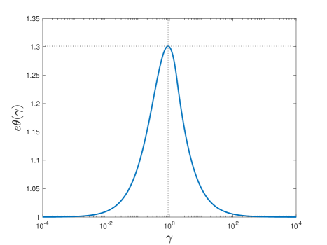
Figure 1: The approximation factor of the mechanism $(\bm{\hat{q}},\bm{\hat{m}})$ as a function of the equity level $\gamma$.

Remark 4.8 (Set-aside Interpretation)

The mechanism $(\hat{\bm{q}},\hat{\bm{m}})$ employs a set-aside implementation. The allocation rule $\hat{\bm{q}}$ can be equivalently expressed as:

$$\hat{q}_{i}(\bm{v})=\frac{1}{1+\gamma}\hat{q}_{i}^{\text{all}}(\bm{v})+\frac{\gamma}{1+\gamma}\hat{q}_{i}^{\text{min}}(\bm{v})\;\;\;\forall i\in\mathcal{I},$$

where

$$\hat{q}_{i}^{\text{all}}(\bm{v})=\begin{cases}\left(1+\log{\overline{\ell}(\bm{v})}\right)^{+}&\text{if }i=\min\arg\max_{j\in\mathcal{I}}v_{j}\\ 0&\text{otherwise,}\end{cases}$$

and

$$\hat{q}_{i}^{\text{min}}(\bm{v})=\begin{cases}\left(1+\log{\overline{\ell}(\bm{v})}\right)^{+}&\text{if }i=\min\arg\max_{j\in\operatorname{\mathcal{I}^{\text{min}}}}v_{j}\\ 0&\text{otherwise,}\end{cases}$$

and $\overline{\ell}(\bm{v})$ represents the maximum revenue achievable in hindsight, that is, it is equal to (1). We note that $\overline{\ell}(\bm{v})={\ell}(\bm{v})$ if $v_{{i^{\text{maj}}(\bm{v})}}>v_{{i^{\text{min}}(\bm{v})}}$ and $\overline{\ell}(\bm{v})=v_{{i^{\text{min}}(\bm{v})}}$ if $v_{{i^{\text{maj}}(\bm{v})}}\leq v_{{i^{\text{min}}(\bm{v})}}$. Note that $\hat{\bm{q}}^{\text{min}}$ allocates exclusively to the minority group. Therefore, the allocation $\hat{\bm{q}}$ reserves a fraction of goods, specifically $\frac{\gamma}{1+\gamma}$, for allocation to the minority group. The payment rule $\hat{\bm{m}}$ can similarly be expressed as $\frac{1}{1+\gamma}\hat{\bm{m}}^{\text{all}}(\bm{v})+\frac{\gamma}{1+\gamma}\hat{\bm{m}}^{\text{min}}(\bm{v})$, where $\hat{\bm{m}}^{\text{all}}$ and $\hat{\bm{m}}^{\text{min}}$ are defined according to Lemma 2.2(ii) as functions of $\hat{\bm{q}}^{\text{all}}$ and $\hat{\bm{q}}^{\text{min}}$, respectively. $\Box$

5 Numerical Illustration

We now numerically assess the performance of the stochastically optimal mechanism $(\bm{q}^{\star},\bm{m}^{\star})$ from Section 3 and the regret-based robust mechanism $(\hat{\bm{q}},\hat{\bm{m}})$ from Section 4. Throughout this numerical illustration, we assume there are $I=2$ bidders: one minority bidder (bidder $1$) and one majority bidder (bidder $2$). We set the equity level $\gamma=\frac{1}{4}$. The mechanism $(\bm{q}^{\star},\bm{m}^{\star})$ is derived from a crisp (but possibly misspecified) value distribution $\mathbb{F}$. We assume that bidders’ values are mutually independent under $\mathbb{F}$ and that its marginals are beta distributions, each with shape parameters equal to $2$, i.e., $\mathbb{F}_{1}=\operatorname{Beta}(2,2)$ and $\mathbb{F}_{2}=\operatorname{Beta}(2,2)$, respectively. The density of $\operatorname{Beta}(2,2)$ is bell-shaped and symmetric and thus resembles the normal distribution. In addition, it has a bounded support $\mathcal{V}=[0,1]$. The robust mechanism $(\hat{\bm{q}},\hat{\bm{m}})$ can be obtained without knowing $\mathbb{F}$.

In practice, the estimated (in-sample) distribution is likely to be subject to estimation errors. In other words, the true (out-of-sample) distribution of the bidders’ values $\tilde{\bm{v}}$ may deviate from the estimated distribution $\mathbb{F}$. To capture this, we assume that the true distribution is representable as $\mathbb{F}^{\epsilon,\rho}=(1-\epsilon)\mathbb{F}+\epsilon\mathbb{B}^{\rho}$, where $\epsilon\in[0,1]$ represents the contamination level, and $\mathbb{B}^{\rho}$, $\rho\in[-1,+1]$, denotes an extremal distribution to be defined below. The distribution $\mathbb{F}^{\epsilon,\rho}$ is a contaminated version of $\mathbb{F}$, where smaller values of $\epsilon$ indicate greater confidence in the estimated distribution $\mathbb{F}$, while larger values indicate lower confidence.

We define the extremal distribution $\mathbb{B}^{\rho}$ as the distribution of two (potentially non-independent) Bernoulli random variables, under which

$$(\tilde{v}_{1},\tilde{v}_{2})=\begin{cases}(0,0)&\text{ with probability }\frac{1+\rho}{4}\\ (0,1)&\text{ with probability }\frac{1-\rho}{4}\\ (1,0)&\text{ with probability }\frac{1-\rho}{4}\\ (1,1)&\text{ with probability }\frac{1+\rho}{4}.\end{cases}$$

Note that $\tilde{v}_{1}$ and $\tilde{v}_{2}$ may not be independent under $\mathbb{B}^{\rho}$, depending on the value of $\rho$, which can be interpreted as a correlation parameter. Additionally, the distribution $\mathbb{B}^{\rho}$ is discrete. Thus, unlike $\mathbb{F}$, $\mathbb{B}^{\rho}$ is not regular. As a result, the distribution $\mathbb{F}^{\epsilon,\rho}$ is also irregular, except when $\epsilon=0$.

We evaluate the performance of the mechanisms $(\bm{q}^{\star},\bm{m}^{\star})$ and $(\hat{\bm{q}},\hat{\bm{m}})$ primarily in terms of the revenue they generate and the regret they incur. This evaluation follows a stress-test approach, conducted on the distribution $\mathbb{F}^{\epsilon,\rho}$, which may differ from $\mathbb{F}$. For comprehensiveness, we introduce two other benchmark mechanisms:

• Inspired by Pai and Vohra (2012) and Fallah et al. (2024), we consider a variant of (S-MDP) that enforces equity only in expectation, i.e., the original (Eq) is replaced by

  $$\mathbb{E}_{\mathbb{F}}\left[\sum_{i\in\mathcal{I}^{\text{min}}}q_{i}(\tilde{\bm{v}})\right]\geq\gamma\mathbb{E}_{\mathbb{F}}\left[\sum_{i\in\mathcal{I}^{\text{maj}}}q_{i}(\tilde{\bm{v}})\right].$$

  The resulting mechanism design problem is a relaxation of (S-MDP), and we denote the optimal mechanism of this relaxed problem as $(\overline{\bm{q}},\overline{\bm{m}})$.

• We also consider the optimal mechanism $({\bm{q}}^{\epsilon,\rho},{\bm{m}}^{\epsilon,\rho})$ in (S-MDP), which is tailored to the true distribution $\mathbb{F}^{\epsilon,\rho}$. We emphasize that this mechanism cannot be realistically computed because, in practice, the distribution of bidders’ values is not known and estimation errors are inevitable.

We remark that the mechanism $(\overline{\bm{q}},\overline{\bm{m}})$ may lie outside $\mathcal{M}$ and fail to be fair ex-post. Additionally, to the best of our knowledge, no closed-form expression exists for $(\overline{\bm{q}},\overline{\bm{m}})$. Likewise, our analytical characterization of $({\bm{q}}^{\star},{\bm{m}}^{\star})$ does not straightforwardly extend to $({\bm{q}}^{\epsilon,\rho},{\bm{m}}^{\epsilon,\rho})$ due to the irregularity of $\mathbb{F}^{\epsilon,\rho}$. Hence, unlike $(\bm{q}^{\star},\bm{m}^{\star})$ and $(\hat{\bm{q}},\hat{\bm{m}})$, we must resort to a numerical approach to find $(\overline{\bm{q}},\overline{\bm{m}})$ and $({\bm{q}}^{\epsilon,\rho},{\bm{m}}^{\epsilon,\rho})$. Since the respective mechanism design problems are infinite-dimensional linear programs, we solve a discrete approximation. Specifically, we approximate $\mathcal{V}^{I}$ by the grid $\hat{\mathcal{V}}^{I}=\mathcal{V}^{I}\cap\delta\mathbb{Z}^{I}$, where $\delta=0.01$, and assign each grid point the probability mass of its lower-left grid area under $\mathbb{F}$. The discrete approximation of distribution $\mathbb{F}^{\epsilon,\rho}$ is obtained by replacing $\mathbb{F}$ with its discrete approximation in the construction of $\mathbb{F}^{\epsilon,\rho}$. The resulting finite-dimensional linear programs are then solved in MATLAB R2024a via the YALMIP interface (Löfberg 2004) and the MOSEK solver (MOSEK ApS 2024). We remark that this discretization scheme for computing $(\overline{\bm{q}},\overline{\bm{m}})$ and $({\bm{q}}^{\epsilon,\rho},{\bm{m}}^{\epsilon,\rho})$ is only reasonably accurate and computationally efficient when the number of bidders $I$ is small. In contrast, our proposed mechanisms $(\bm{q}^{\star},\bm{m}^{\star})$ and $(\hat{\bm{q}},\hat{\bm{m}})$ are available in closed form for any $I$.

In our experiment, we first set $\rho=0$ and consider $\epsilon\in\{0,0.1,\dots,1\}$. We compute the expected revenues of the four mechanisms under the discrete approximation of the distribution $\mathbb{F}^{\epsilon,0}$. Note that the mechanism $({\bm{q}}^{\epsilon,\rho},{\bm{m}}^{\epsilon,\rho})$ must be recomputed every time $\epsilon$ (or $\rho$) changes. We use the expected revenue of $({\bm{q}}^{\epsilon,\rho},{\bm{m}}^{\epsilon,\rho})$ to normalize the expected revenues of the remaining three mechanisms. By construction, the revenues of $(\bm{q}^{\star},\bm{m}^{\star})$ and $(\hat{\bm{q}},\hat{\bm{m}})$ cannot exceed that of $({\bm{q}}^{\epsilon,\rho},{\bm{m}}^{\epsilon,\rho})$, because the discrete approximation relaxes the original constraints of $\mathcal{M}$, and our approximation of the distribution favors $({\bm{q}}^{\epsilon,\rho},{\bm{m}}^{\epsilon,\rho})$ in terms of expected revenues. Therefore, the normalized revenues of $(\bm{q}^{\star},\bm{m}^{\star})$ and $(\hat{\bm{q}},\hat{\bm{m}})$ cannot exceed one. In fact, the revenues of $(\bm{q}^{\star},\bm{m}^{\star})$ and $({\bm{q}}^{\epsilon,\rho},{\bm{m}}^{\epsilon,\rho})$ do not necessarily match even when $\epsilon=0$ due to discretization, which favors the latter. The comparison between $({\bm{q}}^{\epsilon,\rho},{\bm{m}}^{\epsilon,\rho})$ and $(\overline{\bm{q}},\overline{\bm{m}})$ is less straightforward because $(\overline{\bm{q}},\overline{\bm{m}})$ is only required to satisfy the equity constraint in expectation. For this reason, the normalized revenue of $(\overline{\bm{q}},\overline{\bm{m}})$ can exceed $1$. However, this potential excess revenue comes at the cost of violating the equity constraint (Eq). In fact, the probability that $\sum_{i\in\mathcal{I}^{\text{min}}}\overline{q}_{i}(\tilde{\bm{v}})<\gamma\sum_{i\in\mathcal{I}^{\text{maj}}}\overline{q}_{i}(\tilde{\bm{v}})$ is estimated to be $0.46$ under $\mathbb{F}$, implying a significant chance that the equity constraint fails to hold ex-post.

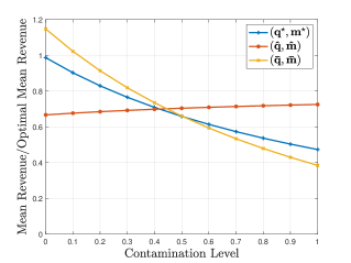
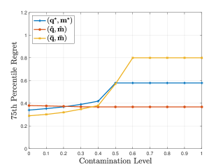
Figure 2: Normalized expected revenues (left) and the upper quartile regrets (right) of the three mechanisms when $\rho=0$: the stochastically optimal mechanism $(\bm{q}^{\star},\bm{m}^{\star})$ (blue), its variant $(\overline{\bm{q}},\overline{\bm{m}})$ that enforces equity only in expectation (yellow), and the regret-based mechanism $(\hat{\bm{q}},\hat{\bm{m}})$ (red).

Figure 2 (left) illustrates the normalized expected revenues, and Figure 2 (right) displays the 75th percentile regrets for different mechanisms and contamination levels. From both the revenue and regret plots, we find (unsurprisingly) that the stochastically optimal mechanism $(\bm{q}^{\star},\bm{m}^{\star})$ outperforms the regret-based mechanism $(\hat{\bm{q}},\hat{\bm{m}})$ when the contamination level $\epsilon$ is small. However, we observe that both the expected revenue and the 75th percentile regret of $(\hat{\bm{q}},\hat{\bm{m}})$ remain relatively stable across different contamination levels, highlighting the robustness of the mechanism, and actually outperform those of $(\bm{q}^{\star},\bm{m}^{\star})$ and $(\overline{\bm{q}},\overline{\bm{m}})$ as $\epsilon$ increases. Interestingly, the performance of the mechanism $(\overline{\bm{q}},\overline{\bm{m}})$ deteriorates significantly (more so in comparison to $(\bm{q}^{\star},\bm{m}^{\star})$) as $\epsilon$ increases. We attribute this to the mechanism’s high reliance on the (incorrect) distribution $\mathbb{F}$ in both the objective and the feasible set. Compared to the other mechanisms, it is more prone to overfitting.

We then repeat the experiment for other $\rho$ values from $\{0.5,-0.5\}$, and the obtained results are presented in Appendix B. Similar observations can be made for these cases. We observe that, as the contamination level $\epsilon$ grows, the decline in the performance of $(\bm{q}^{\star},\bm{m}^{\star})$ and $(\overline{\bm{q}},\overline{\bm{m}})$ is faster when $\rho$ is negative and slower when $\rho$ is positive. The performance of the regret-based mechanism $(\hat{\bm{q}},\hat{\bm{m}})$ remains relatively stable.

Acknowledgment:

This research was supported by the Ministry of Education, Singapore, under its Academic Research Fund Tier 2 grant MOE-T2EP20222-0003 and Academic Research Fund Tier 3 grant MOE-2019-T3-1-010.

Appendix

A Proofs

Proof A.1

Proof of Lemma 3.1 By utilizing Lemma 2.2 and noting that $m_{i}(0,\bm{v}_{-i})=0$ holds for all $i\in\mathcal{I}$ and $\bm{v}_{-i}\in\mathcal{V}^{I-1}$ at optimality, we can reformulate problem (S-MDP) equivalently as follows.

$$\max \mathbb{E}_{\mathbb{F}}\left[\sum_{i\in\mathcal{I}}\left(q_{i}(\tilde{\bm{v}})\tilde{v}_{i}-\int_{0}^{\tilde{v}_{i}}q_{i}(x,\tilde{\bm{v}}_{-i})\text{d}x\right)\right]$$ (13)

  s.t. $$\bm{q}\in\mathcal{L}(\mathcal{V}^{I},[0,1]^{I}),\;\bm{m}\in\mathcal{L}(\mathcal{V}^{I},\mathbb{R}^{I})$$

$$q_{i}(v_{i},\bm{v}_{-i})\geq q_{i}(w_{i},\bm{v}_{-i})\;\;\;\forall i\in\mathcal{I},\forall\bm{v}\in\mathcal{V}^{I},\forall w_{i}\in\mathcal{V}:w_{i}\leq v_{i}$$

$$m_{i}(\bm{v})=q_{i}(\bm{v})v_{i}-\int_{0}^{{v}_{i}}q_{i}(x,\bm{v}_{-i})\text{d}x\;\;\;\forall i\in\mathcal{I},\forall\bm{v}\in\mathcal{V}^{I}$$

$$\eqref{eq:AF},\,\eqref{eq:Eq}$$

Let $f$ denote the joint density function of $\tilde{\bm{v}}$. The objective function of (13) can then be expressed in terms of $f$ and simplified as follows:

$$\mathbb{E}_{\mathbb{F}}\left[\sum_{i\in\mathcal{I}}\left(q_{i}(\tilde{\bm{v}})\tilde{v}_{i}-\int_{0}^{\tilde{v}_{i}}q_{i}(x,\tilde{\bm{v}}_{-i})\text{d}x\right)\right]$$ (14)

$$= \sum_{i\in\mathcal{I}}\left(\int_{\mathcal{V}^{I-1}}\int_{\mathcal{V}}q_{i}({\bm{v}}){v}_{i}f(\bm{v})\text{d}v_{i}\text{d}\bm{v}_{-i}-\int_{\mathcal{V}^{I-1}}\int_{\mathcal{V}}\int_{0}^{{v}_{i}}q_{i}(x,{\bm{v}}_{-i})\text{d}xf(\bm{v})\text{d}v_{i}\text{d}\bm{v}_{-i}\right)$$

$$= \sum_{i\in\mathcal{I}}\left(\int_{\mathcal{V}^{I-1}}\int_{\mathcal{V}}q_{i}({\bm{v}}){v}_{i}f(\bm{v})\text{d}v_{i}\text{d}\bm{v}_{-i}-\int_{\mathcal{V}^{I-1}}\int_{\mathcal{V}}\int_{0}^{x}q_{i}(v_{i},{\bm{v}}_{-i})\text{d}v_{i}f(x,\bm{v}_{-i})\text{d}x\text{d}\bm{v}_{-i}\right)$$

$$= \sum_{i\in\mathcal{I}}\left(\int_{\mathcal{V}^{I-1}}\int_{\mathcal{V}}q_{i}({\bm{v}}){v}_{i}f(\bm{v})\text{d}v_{i}\text{d}\bm{v}_{-i}-\int_{\mathcal{V}^{I-1}}\int_{\mathcal{V}}q_{i}(v_{i},{\bm{v}}_{-i})\left(\int_{v_{i}}^{1}f(x,\bm{v}_{-i})\text{d}x\right)\text{d}v_{i}\text{d}\bm{v}_{-i}\right)$$

$$= \sum_{i\in\mathcal{I}}\int_{\mathcal{V}^{I-1}}\int_{\mathcal{V}}\left(v_{i}-\frac{\int_{v_{i}}^{1}f(x,\bm{v}_{-i})\text{d}x}{f(\bm{v})}\right)q_{i}({\bm{v}})f(\bm{v})\text{d}v_{i}\text{d}\bm{v}_{-i},$$

where the second equality follows from relabeling the variable $x$ as $v_{i}$ and vice versa, and the third equality results from swapping the order of integration over $x$ and $v_{i}$, which is justified by Fubini’s theorem.

Next, we recall the definition of the virtual values

$$\psi_{i}(v_{i})=v_{i}-\frac{1-\int_{0}^{{v}_{i}}f_{i}(x)\text{d}x}{f_{i}(v_{i})}=v_{i}-\frac{\int_{v_{i}}^{1}f_{i}(x)\text{d}x}{f_{i}(v_{i})}=v_{i}-\frac{\int_{v_{i}}^{1}f(x,\bm{v}_{-i})\text{d}x}{f(\bm{v})}\;\;\;\forall\bm{v}\in\mathcal{V}^{I},$$

where the transition from marginal density function $f_{i}$ to the joint density function $f$ in the rightmost equation is valid when the bidder’s values are independent. Using this observation and the equation (14), we can finally re-express the objective of (13) as

$$\sum_{i\in\mathcal{I}}\int_{\mathcal{V}^{I-1}}\int_{\mathcal{V}}\psi_{i}(v_{i})q_{i}({\bm{v}})f(\bm{v})\text{d}v_{i}\text{d}\bm{v}_{-i}=\mathbb{E}_{\mathbb{F}}\left[\sum_{i\in\mathcal{I}}\psi_{i}(\tilde{v}_{i})q_{i}(\tilde{\bm{v}})\right],$$

which completes the proof. $\square$

Proof A.2

Proof of Proposition 3.2 We will first prove that the constraint (IC) holds under the mechanism $(\bm{q}^{\star},\bm{m}^{\star})$ for both minority bidders (Case 1) and majority bidders (Case 2). Then, we will prove constraints  (IR), (AF) and  (Eq) and conclude the proof.

To prove that $(\bm{q}^{\star},\bm{m}^{\star})$ satisfies the (IC) constraint, it is sufficient to show that conditions (i) and (ii) in Lemma 2.2 hold. By definition of $\bm{m}^{\star}$, condition (ii) in Lemma 2.2 immediately holds. We now consider (i) and show that the allocation rule $\bm{q}^{\star}$ is non-decreasing, that is, for each $i\in\mathcal{I}$, it holds that $q^{\star}_{i}(v_{i},\bm{v}_{-i})\geq q^{\star}_{i}(w_{i},\bm{v}_{-i})$ for all $\bm{v}\in\mathcal{V}^{I}$ and $w_{i}\in\mathcal{V}:v_{i}\geq w_{i}$. Suppose for the sake of finding a contradiction that $q^{\star}_{i}(v_{i},\bm{v}_{-i})<q^{\star}_{i}(w_{i},\bm{v}_{-i})$ for some $\bm{v}\in\mathcal{V}^{I}$, $w_{i}\in\mathcal{V}$ such that $v_{i}\geq w_{i}$, and consider two cases.

Case 1 ($i\in\operatorname{\mathcal{I}^{\text{min}}}$): If $0\leq q^{\star}_{i}(v_{i},\bm{v}_{-i})<q^{\star}_{i}(w_{i},\bm{v}_{-i})$, by definition of $\bm{q}^{\star}$, we must have $q_{i}(w_{i},\bm{v}_{-i})=1$ or $q_{i}(w_{i},\bm{v}_{-i})=\frac{\gamma}{1+\gamma}$. Suppose first that $q^{\star}_{i}(w_{i},\bm{v}_{-i})=1$. By definition of $\bm{q}^{\star}$, in this case, $i$ must be the smallest index of the bidders with the highest and non-negative virtual value. As $v_{i}>w_{i}$ and as $\psi_{i}$ is non-decreasing by Assumption 3, $\psi_{i}(v_{i})\geq 0$ and $\psi_{i}(v_{i})=\max_{j\in\mathcal{I}}\psi_{j}(v_{j})$. Hence, $q^{\star}_{i}(v_{i},\bm{v}_{-i})=1$ which coincides with $q^{\star}_{i}(w_{i},\bm{v}_{-i})$, leading to a contradiction. Suppose next that $q^{\star}_{i}(w_{i},\bm{v}_{-i})=\frac{\gamma}{1+\gamma}$. In this case, $i$ must represent the bidder with the highest virtual value from the minority group, and it must hold that

$$\max_{j\in\operatorname{\mathcal{I}^{\text{maj}}}}\psi_{j}(v_{j})>\psi_{i}(w_{i})\quad\text{and}\quad\max_{j\in\operatorname{\mathcal{I}^{\text{maj}}}}\psi_{j}(v_{j})+\gamma\psi_{i}(w_{i})\geq 0.$$

The second inequality continues to hold when $\psi_{i}(w_{i})$ is replaced by $\psi_{i}(v_{i})$. If the first inequality also remains satisfied after a similar substitution $\psi_{i}(v_{i})$ for $\psi_{i}(w_{i})$, then $q^{\star}_{i}(v_{i},\bm{v}_{-i})=\frac{\gamma}{1+\gamma}=q^{\star}_{i}(w_{i},\bm{v}_{-i})$ resulting in a contradiction. On the other hand, if $\psi_{i}(v_{i})\geq\max_{j\in\operatorname{\mathcal{I}^{\text{maj}}}}\psi_{j}(v_{j})$, then $i$ must be the bidder with the highest virtual value among all bidders and

$$(1+\gamma)\psi_{i}(v_{i})\geq\max_{j\in\operatorname{\mathcal{I}^{\text{maj}}}}\psi_{j}(v_{j})+\gamma\psi_{i}(v_{i})\geq\max_{j\in\operatorname{\mathcal{I}^{\text{maj}}}}\psi_{j}(v_{j})+\gamma\psi_{i}(w_{i})\geq 0.$$

As a result, $q^{\star}_{i}(v_{i},\bm{v}_{-i})=1\geq q^{\star}_{i}(w_{i},\bm{v}_{-i})$ resulting in another contradiction.

Case 2 ($i\in\operatorname{\mathcal{I}^{\text{maj}}}$): If $0\leq q^{\star}_{i}(v_{i},\bm{v}_{-i})<q^{\star}_{i}(w_{i},\bm{v}_{-i})$, by definition of $\bm{q}^{\star}$, we must have $q_{i}(w_{i},\bm{v}_{-i})=\frac{1}{1+\gamma}$. It hence follows that

$$\psi_{i}(w_{i})\geq\max_{j\in\mathcal{I}}\psi_{j}(v_{j})\quad\text{and}\quad\psi_{i}(w_{i})+\gamma\max_{j\in\operatorname{\mathcal{I}^{\text{min}}}}\psi_{j}(v_{j})\geq 0.$$

Since $v_{i}>w_{i}$ and $\psi_{i}$ is non-decreasing by Assumption 3, $i$ remains the highest majority bidder in scenario $(v_{i},\bm{v}_{-i})$, and the above two inequalities continue to hold even if $\psi_{i}(w_{i})$ is replaced by $\psi_{i}(v_{i})$. Hence, it must also hold that $q^{\star}_{i}(v_{i},\bm{v}_{-i})=\frac{1}{1+\gamma}$ and a similar contradiction is found.

Constraint (IR) holds immediately because $q_{i}(\bm{v})v_{i}-m_{i}(\bm{v})=\int_{0}^{{v}_{i}}q_{i}(x,\bm{v}_{-i})\text{d}x\geq 0$ for all $i\in\mathcal{I}$ and $\bm{v}\in\mathcal{V}^{I}$.

Constraint (AF) is also trivially satisfied. Indeed, if a bidder with the highest virtual value is from the minority group, then the good can be allocated to neither the majority group nor any minority bidder with dominated virtual values. On the other hand, if this bidder comes from the majority group, then $\sum_{i\in\mathcal{I}}q_{i}^{\star}(\bm{v})$ cannot exceed $\frac{\gamma}{1+\gamma}+\frac{1}{1+\gamma}=1$.

Finally, we prove (Eq). Suppose for the sake of contradiction that (Eq) does not hold for some $\bm{v}\in\mathcal{V}$. Then, it must hold that $\sum_{i\in\mathcal{I}^{\text{maj}}}q^{\star}_{i}(\bm{v})=\frac{1}{1+\gamma}$ and $\sum_{i\in\mathcal{I}^{\min}}q^{\star}_{i}(\bm{v})<\frac{\gamma}{1+\gamma}$, and hence, $q^{\star}_{i}(\bm{v})=0,\ \forall i\in\mathcal{I}^{\min}$. Since the total allocation to the majority group $\sum_{i\in\mathcal{I}^{\text{maj}}}q^{\star}_{i}(\bm{v})=\frac{1}{1+\gamma}$, $\min\arg\max_{j\in\mathcal{I}}\psi_{j}(v_{j})\in\mathcal{I}^{\text{maj}}$ and $\psi_{i}(v_{i})+\gamma\max_{j\in\mathcal{I}^{\text{min}}}\psi_{j}(v_{j})\geq 0$. Thus, the allocation to the bidder with the largest virtual value in the minority group is $\frac{\gamma}{1+\gamma}$, leading to a contradiction. The claim thus follows. $\square$

Proof A.3

Proof of Proposition 4.3 We will first prove that the constraint (IC) holds under the mechanism $(\bm{\hat{q}},\bm{\hat{m}})$ for both minority bidders (Case 1) and majority bidders (Case 2). Then, we will prove constraints  (IR), (Eq) and  (AF) and conclude the proof.

To prove that $(\bm{\hat{q}},\bm{\hat{m}})$ satisfies the (IC) constraint, it is sufficient to show that conditions (i) and (ii) in Lemma 2.2 hold. By definition of $\bm{\hat{m}}$, condition (ii) in Lemma 2.2 immediately holds. Hence, it remains to establish condition (i), that is, to show that the allocation rule ${\hat{q}}_{i}$ is non-decreasing in $v_{i}$ for all $i\in\mathcal{I}$.

Case 1 ($i\in\operatorname{\mathcal{I}^{\text{min}}}$): Assume that $i\in\mathcal{I}^{\text{min}}$. By construction, we can re-express the allocation $\hat{q}_{i}$ as

$$\hat{q}_{i}(\bm{v}) =\begin{cases}\dfrac{\gamma}{1+\gamma}\left(1+\log{\ell(\bm{v})}\right)^{+}\mathbb{I}_{\{i={i^{\text{min}}(\bm{v})}\}}&\text{ if }v_{i}<v_{{i^{\text{maj}}(\bm{v})}}\\ (1+\log v_{i})^{+}\mathbb{I}_{\{i={i^{\text{min}}(\bm{v})}\}}&\text{ otherwise. }\end{cases}$$

Note that for a given $\bm{v}_{-i}$, both $\ell(\bm{v})$ and the indicator function $\mathbb{I}_{\{i={i^{\text{min}}(\bm{v})}\}}$ are non-decreasing in $v_{i}$. Since $\log{x}$ is also a non-decreasing function, our $\hat{q}_{i}(\bm{v})$ is non-decreasing in intervals $[0,v_{{i^{\text{maj}}(\bm{v})}})$ and $(v_{{i^{\text{maj}}(\bm{v})}},1]$. It is now evident that $\hat{q}_{i}$ is non-decreasing in $v_{i}\in\mathcal{V}$ as

$$\sup_{v_{i}<v_{{i^{\text{maj}}(\bm{v})}}}\dfrac{\gamma}{1+\gamma}\left(1+\log{\ell(\bm{v})}\right)^{+}\mathbb{I}_{\{i={i^{\text{min}}(\bm{v})}\}}=\dfrac{\gamma}{1+\gamma}\left(1+\log v_{{i^{\text{maj}}(\bm{v})}}\right)^{+}\mathbb{I}_{\{i={i^{\text{min}}(\bm{v})}\}}$$

$$\leq\left(1+\log v_{{i^{\text{maj}}(\bm{v})}}\right)^{+}\mathbb{I}_{\{i={i^{\text{min}}(\bm{v})}\}}=\inf_{v_{i}\geq v_{{i^{\text{maj}}(\bm{v})}}}\left(1+\log v_{i}\right)^{+}\mathbb{I}_{\{i={i^{\text{min}}(\bm{v})}\}}.$$

Case 2 ($i\in\operatorname{\mathcal{I}^{\text{maj}}}$): Assume next that $i\in\mathcal{I}^{\text{maj}}$. We can similarly express the allocation $\hat{q}_{i}$ as

$$\hat{q}_{i}(\bm{v}) =\begin{cases}\dfrac{1}{1+\gamma}\left(1+\log{\ell(\bm{v})}\right)^{+}\mathbb{I}_{\{i={i^{\text{maj}}(\bm{v})}\}}&\text{ if }v_{i}>v_{{i^{\text{min}}(\bm{v})}}\\ 0&\text{ otherwise. }\end{cases}$$

Similarly, as $\ell(\bm{v})$ and the indicator function $\mathbb{I}_{\{i={i^{\text{maj}}(\bm{v})}\}}$ are non-decreasing in $v_{i}$, it can be seen that $\hat{q}_{i}$ is non-decreasing in $v_{i}$.

Constraints  (IR), (Eq) and  (AF) trivially hold due to the construction of the mechanism $(\bm{\hat{q}},\bm{\hat{m}})$. Indeed, this mechanism is individually rational because

$$v_{i}{\hat{q}}_{i}(\bm{v})-{\hat{m}}_{i}(\bm{v})=\int_{0}^{v_{i}}{\hat{q}}_{i}(x,\bm{v}_{-i}){\rm{d}}x\geq 0\quad\forall i\in\mathcal{I},$$

and it is equitable as

$$\sum_{i\in\mathcal{I}^{\text{min}}}{\hat{q}}_{i}(\bm{v})=\begin{cases}\dfrac{\gamma}{1+\gamma}\left(1+\log{\ell(\bm{v})}\right)^{+}&\text{ if }v_{{i^{\text{maj}}(\bm{v})}}>v_{{i^{\text{min}}(\bm{v})}}\\ \left(1+\log v_{{i^{\text{min}}(\bm{v})}}\right)^{+}&\text{ otherwise,}\end{cases}$$

and

$$\sum_{i\in\mathcal{I}^{\text{maj}}}{\hat{q}}_{i}(\bm{v})=\begin{cases}\dfrac{1}{1+\gamma}\left(1+\log{\ell(\bm{v})}\right)^{+}&\text{ if }v_{{i^{\text{maj}}(\bm{v})}}>v_{{i^{\text{min}}(\bm{v})}}\\ 0&\text{ otherwise.}\end{cases}$$

From $\sum_{i\in\mathcal{I}^{\text{min}}}{\hat{q}}_{i}(\bm{v})$ and $\sum_{i\in\mathcal{I}^{\text{maj}}}{\hat{q}}_{i}(\bm{v})$ computed above, we also obtain

$$\sum_{i\in\mathcal{I}}{\hat{q}}_{i}(\bm{v})=\sum_{i\in\mathcal{I}^{\text{min}}}{\hat{q}}_{i}(\bm{v})+\sum_{i\in\mathcal{I}^{\text{maj}}}{\hat{q}}_{i}(\bm{v})=\begin{cases}\left(1+\log{\ell(\bm{v})}\right)^{+}&\text{ if }v_{{i^{\text{maj}}(\bm{v})}}>v_{{i^{\text{min}}(\bm{v})}}\\ \left(1+\log v_{{i^{\text{min}}(\bm{v})}}\right)^{+}&\text{ otherwise,}\end{cases}$$

and hence the total allocation probability does not exceed one as both $\ell(\bm{v})$ and $v_{i^{\text{min}}(\bm{v})}$ belong to $\mathcal{V}$.

As the mechanism $(\bm{\hat{q}},\bm{\hat{m}})$ satisfies all constraints in $\mathcal{M}$, the claim follows. $\square$

B Supplementary Numerical Results

In this section, we repeat the experiment from Section 5 for $\rho$ values from $\{0.5,-0.5\}$ and show the results in Figures 3 and 4, respectively. We observe that the results are similar to the case where $\rho=0$ (see Figure 2), where the regret-based mechanism exhibits the most stable performance across different contamination levels.

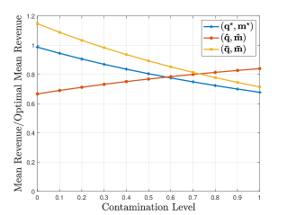
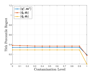
Figure 3: Normalized expected revenues (left) and the upper quartile regrets (right) of the three mechanisms when $\rho=0.5$: the stochastically optimal mechanism $(\bm{q}^{\star},\bm{m}^{\star})$ (blue), its variant $(\overline{\bm{q}},\overline{\bm{m}})$ that enforces equity only in expectation (yellow), and the regret-based mechanism $(\hat{\bm{q}},\hat{\bm{m}})$ (red).

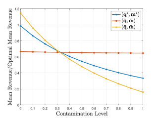
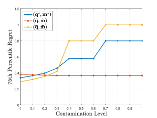
Figure 4: Normalized expected revenues (left) and the upper quartile regrets (right) of the three mechanisms when $\rho=-0.5$: the stochastically optimal mechanism $(\bm{q}^{\star},\bm{m}^{\star})$ (blue), its variant $(\overline{\bm{q}},\overline{\bm{m}})$ that enforces equity only in expectation (yellow), and the regret-based mechanism $(\hat{\bm{q}},\hat{\bm{m}})$ (red).

References

- (1)
- Anunrojwong et al. (2023) Jerry Anunrojwong, Santiago R Balseiro, and Omar Besbes. 2023. Robust auction design with support information. (2023). Preprint, submitted May 15, https://arxiv.org/abs/2305.09065.
- Athey et al. (2013) Susan Athey, Dominic Coey, and Jonathan Levin. 2013. Set-asides and subsidies in auctions. American Economic Journal: Microeconomics 5, 1 (2013), 1–27.
- Bansak and Paulson (2024) Kirk Bansak and Elisabeth Paulson. 2024. Outcome-driven dynamic refugee assignment with allocation balancing. Operations Research 72, 6 (2024), 2375–2390.
- Barman et al. (2018) Siddharth Barman, Sanath Kumar Krishnamurthy, and Rohit Vaish. 2018. Finding fair and efficient allocations. In Proceedings of the 2018 ACM Conference on Economics and Computation. 557–574.
- Bergemann and Schlag (2008) Dirk Bergemann and Karl H Schlag. 2008. Pricing without priors. Journal of the European Economic Association 6, 2-3 (2008), 560–569.
- Chen et al. (2024) Zhi Chen, Zhenyu Hu, and Ruiqin Wang. 2024. Screening with limited information: A dual perspective. Operations Research 72, 4 (2024), 1487–1504.
- Ewerhart (2013) Christian Ewerhart. 2013. Regular type distributions in mechanism design and -concavity. Economic Theory 53, 3 (2013), 591–603.
- Fallah et al. (2024) Alireza Fallah, Michael I Jordan, and Annie Ulichney. 2024. Fair allocation in dynamic mechanism design. (2024). Preprint, submitted May 31, https://arxiv.org/abs/2406.00147.
- Federal Register (2023) Federal Register. 2023. Further Advancing Racial Equity and Support for Underserved Communities Through the Federal Government. https://www.federalregister.gov Accessed: 2025-01-24.
- Freund et al. (2023) Daniel Freund, Thodoris Lykouris, Elisabeth Paulson, Bradley Sturt, and Wentao Weng. 2023. Group fairness in dynamic refugee assignment. In Proceedings of the 24th ACM Conference on Economics and Computation. 701–701.
- Giannakopoulos et al. (2023) Yiannis Giannakopoulos, Diogo Poças, and Alexandros Tsigonias-Dimitriadis. 2023. Robust revenue maximization under minimal statistical information. ACM Transactions on Economics and Computation 10, 3 (2023), 1–34.
- Jo et al. (2023) Nathanael Jo, Bill Tang, Kathryn Dullerud, Sina Aghaei, Eric Rice, and Phebe Vayanos. 2023. Fairness in contextual resource allocation systems: Metrics and incompatibility results. In Proceedings of the AAAI Conference on Artificial Intelligence, Vol. 37. 11837–11846.
- Koçyiğit et al. (2024) Çağıl Koçyiğit, Daniel Kuhn, and Napat Rujeerapaiboon. 2024. Regret Minimization and Separation in Multi-Bidder, Multi-Item Auctions. INFORMS Journal on Computing 36, 6 (2024), 1359–1756.
- Koçyiğit et al. (2022) Çağıl Koçyiğit, Napat Rujeerapaiboon, and Daniel Kuhn. 2022. Robust multidimensional pricing: Separation without regret. Mathematical Programming (2022), 1–34.
- Krishna (2009) Vijay Krishna. 2009. Auction theory. Academic press.
- Löfberg (2004) J. Löfberg. 2004. YALMIP : A Toolbox for Modeling and Optimization in MATLAB. In In Proceedings of the CACSD Conference. Taipei, Taiwan.
- MOSEK ApS (2024) MOSEK ApS. 2024. The MOSEK optimization toolbox for MATLAB manual. Version 10.1. http://docs.mosek.com/latest/toolbox/index.html
- Myerson (1981) Roger B Myerson. 1981. Optimal auction design. Mathematics of Operations Research 6, 1 (1981), 58–73.
- Pai and Vohra (2012) Mallesh M Pai and Rakesh Vohra. 2012. Auction design with fairness concerns: Subsidies vs. set-asides. Technical Report.
- Rujeerapaiboon et al. (2023) Napat Rujeerapaiboon, Yize Wei, and Yilin Xue. 2023. Target-oriented regret minimization for satisficing monopolists. In International Conference on Web and Internet Economics. Springer, 563–581.
- Tang et al. (2023) Bill Tang, Çağıl Koçyiğit, Eric Rice, and Phebe Vayanos. 2023. Learning optimal and fair policies for online allocation of scarce societal resources from data collected in deployment. (2023). Preprint, submitted November 23, https://arxiv.org/abs/2311.13765.
- Wang (2024) Shixin Wang. 2024. The power of simple menus in robust selling mechanisms. Management Science (in press) (2024).