Probing the many-body localized spin-glass phase through quench dynamics
Abstract
Eigenstates of quantum many-body systems are often used to define phases of matter in and out of equilibrium; however, experimentally accessing highly excited eigenstates is a challenging task, calling for alternative strategies to dynamically probe nonequilibrium phases. In this work, we characterize the dynamical properties of a disordered spin chain, focusing on the spin-glass regime. Using tensor-network simulations, we observe oscillatory behavior of local expectation values and bipartite entanglement entropy. We explain these oscillations deep in the many-body localized spin glass regime via a simple theoretical model. From perturbation theory, we predict the timescales up to which our analytical description is valid and confirm it with numerical simulations. Finally, we study the correlation length dynamics, which, after a long-time plateau, resumes growing in line with renormalization group (RG) expectations. Our work suggests that RG predictions can be quantitatively tested against numerical simulations and experiments, potentially enabling microscopic descriptions of dynamical phases in large systems.
Introduction.—The fate of interacting quantum systems evolving under unitary dynamics is an outstanding question in modern quantum many-body physics that has received considerable attention in recent years, both theoretically [1, 2, 3, 4, 5, 6] and experimentally [7, 8, 9, 10, 11, 12, 13]. Generic systems are believed to follow the eigenstate thermalization hypothesis (ETH) [14, 15], resulting in thermal expectation values for local observables at late times. On the other hand, integrable [16] and disordered models show a breakdown of ergodicity and absence of thermalization. While integrability is extremely fragile to perturbations, many-body localized systems [17, 18, 19, 20, 21] provide a robust way of escaping thermalization on experimentally relevant sizes and timescales [22, 23, 24, 25, 26].
More recently, increasing attention has been devoted to the interplay of disorder and topological order [27, 28, 29, 30, 31, 32, 33, 34, 35], as shown e.g. in the interacting Majorana chain. In these systems, the disorder of the local potential and of the bond coupling compete, and two distinct MBL phases emerge [36, 27, 28, 29, 30]. When the on-site disorder dominates, the system is in a paramagnetic MBL phase [30, 28, 29], where the original topological order is completely destroyed and the system behaves according to standard MBL: area-law entanglement of eigenstates [37, 38], Poissonian level statistics [39], and slow entanglement growth [40]. However, in the opposite scenario of dominating bond disorder the system enters a novel MBL phase, characterized by long-range correlations, degeneracies in the spectrum and a cat-like structure of the eigenstates [27, 30, 28, 29] leading to higher entanglement as compared to the paramagnet MBL. In spite of the growing interest, the dynamical characterization of this MBL spin-glass (MBL-SG) phase is still limited to small systems [32].
In this work, we study the dynamics of random product states in the extended Ising model introduced in Refs. [28, 29, 30]. In particular, we focus on the dynamics deep in the MBL-SG phase. We show that this regime is characterized by oscillatory dynamics both in local observables and entanglement entropy. Through an approximate description of the time evolution, we analytically provide accurate predictions for the behavior of magnetization and entanglement. We show that the local magnetization oscillates with frequencies depending on the bond disorder and on the interaction strength. We further explain the bounds on entanglement growth and its oscillations through the matrix-product-operator (MPO) representation of the approximate time propagator [41]. Finally, we extract the correlation length from the exponential decay of the correlation function. Our study shows that the correlation length initially saturates to a finite value, but resumes growing on a timescale scaling exponentially with the disorder strength. The unbounded growth of the correlation length is in line with the long-range order detected in highly excited eigenstates within the MBL-SG phase.
Model.—We study an extended Ising model with random couplings and random transverse fields
| (1) |
where spin-1/2 operators are expressed via Pauli matrices, . In this model the interaction strength sets the scale for the next-nearest-neighbor Ising interaction and for the coupling along the direction. Throughout this paper, we fix the interaction strength to , and we define a disorder parameter , where the bar indicates average over disorder realizations and lattice sites. To avoid introducing large energy scales, we fix .
The model has symmetry, given by . Additionally, the Hamiltonian (1) is self-dual under the transformation , and [32]. The Hamiltonian (1) can further be mapped to an interacting Majorana chain through a Jordan-Wigner transformation to spinless fermions and an additional introduction of Majorana fermions [30].
Previous exact diagonalization (ED) studies of model (1) have shown the emergence of three distinct phases [36, 27, 30, 28, 29]. At large negative , where disorder in the local magnetic field is dominant, there exists a localized paramagnetic phase presenting the characteristic features of standard MBL phases. At intermediate around , the model enters an ergodic phase, characterized by volume-law entanglement entropy of the eigenstates [28, 29, 30]. Finally, at large positive there is a transition to the MBL spin-glass phase. This latter phase has interesting remnant topological features, such as spectral pairing and long-range order in the magnetization [36, 27, 28, 29, 30].
In the remainder of this work we will investigate the dynamics deep in the spin-glass phase, where we can provide an analytical theory explaining our numerical observations. We will focus on the dynamics from random product states in the computational basis that can be easily prepared and probed experimentally in a variety of quantum simulation platforms [13, 42].
Magnetization dynamics.—First, we analyze the local magnetization dynamics . While in the MBL paramagnetic phase the strong local fields favor freezing of the local magnetization close to its initial value, at strong positive bond disorder is dominant and magnetization is expected to vanish [43, 44]. However, we find that the decay of magnetization is not entirely featureless and carries information about the local disorder in the long-lived oscillations that characterize its dynamics.
Deep in the spin-glass phase, , one can neglect the terms containing the operators in the Hamiltonian, resulting in the approximate time propagator
| (2) |
Using this approximation, we analytically obtain for each individual disorder realization [45] as
| (3) |
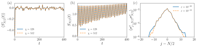
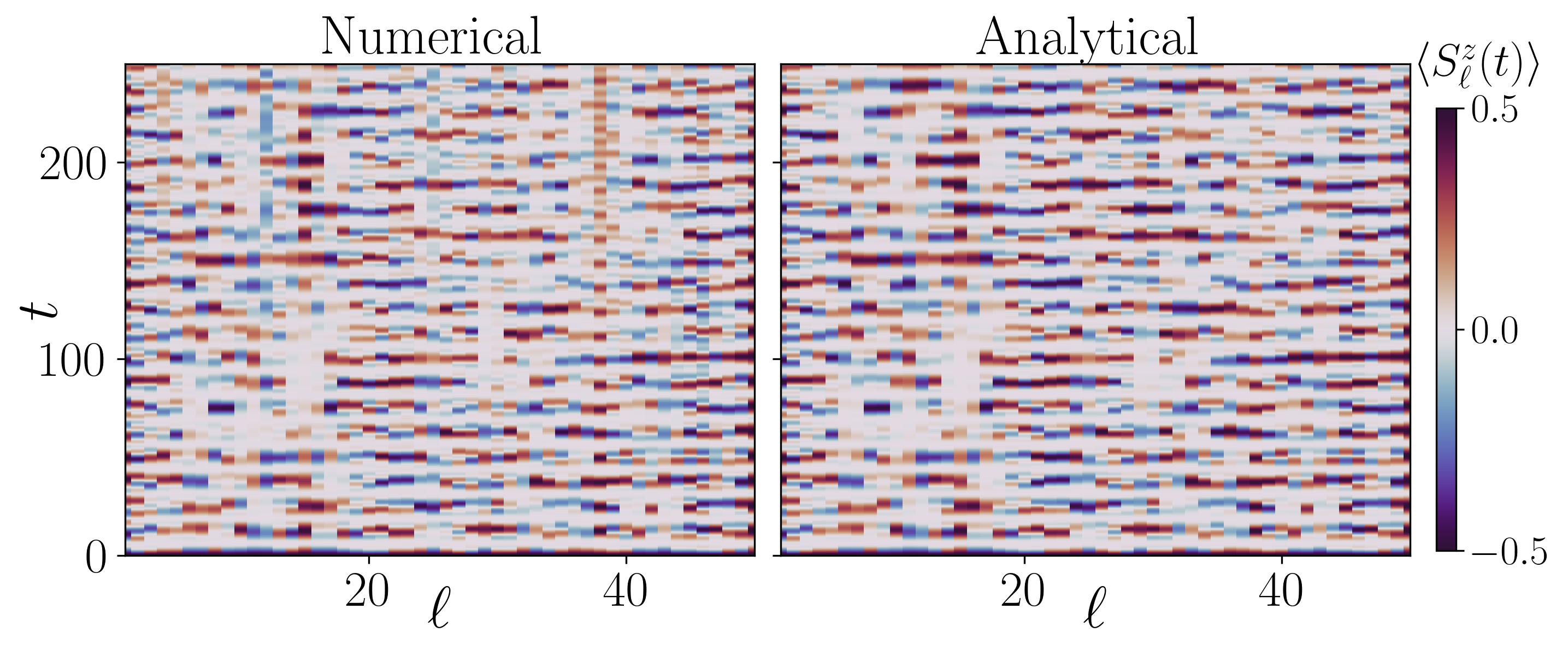
where is the initial value of the magnetization on site . Knowing all disordered couplings we obtain the dynamics of the local magnetization in the system and compare it with our numerical results obtained via time-evolving-block-decimation (TEBD) [46] with bond dimension [45]. As we show in Fig. 1 and in the inset of Fig. 2(b), our analytical prediction captures the quantitative behavior up to times , and continues to describe the dynamics qualitatively at even longer timescales.
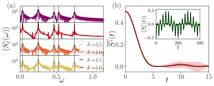
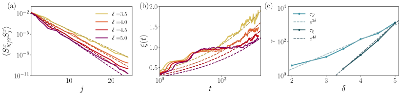
This theoretical result provides a reliable scheme to understand dynamical behaviors in the MBL-SG phase. In particular, Eq. (3) predicts the emergence of oscillations in the magnetization dynamics, with resonant frequencies . The frequencies can be obtained from the Fourier transform of the expression in Eq. (3) , yielding , . In Figure 2(a) we report the Fourier transform of the local magnetization at a given site for a single disorder realization and for different values of within the spin-glass phase. The Fourier signal shows six evident peaks at the frequencies predicted by our analytical results (black dashed lines), with no dependence on the disorder strength .
The analytical expression for obtained above further allows to calculate exact disorder averages. Indeed, each disorder instance produces an independent set of random frequencies determined by and , and the disorder average can be obtained by integrating over the distribution function , where is Heaviside’s theta function. The average local magnetization then reads
| (4) |
Defining the average magnetization for the sites where as and analogously , we obtain the global average magnetization as , analogous to the imbalance introduced in Néel initial states [22, 24]. The exact disorder average shows a fast power law decay of the global magnetization, as expected due to the dominant bond disorder in the MBL spin-glass regime. This can be contrasted to the RG study of the random coupling spin-1/2 XXZ chain [43], where the Neél order parameter decays parametrically slower.
In Figure 2(b) we compare the prediction of Eq. (4) with numerical simulations. The short time decay of agrees well with our analytic expression, confirming the fast decay . At longer times, numerical results still show small oscillations, but within uncertainty their value agrees with the exact disorder average decaying monotonically. In summary our theoretical description accurately captures both the single realization oscillations and the average decay of the local magnetization, thus indicating measurable dynamical features of the MBL-SG phase.
Entanglement dynamics.—Next, we study the behavior of the half-chain entanglement entropy, defined as the von Neumann entropy of the reduced density matrix , where and are the two halves of the chain, . Entanglement entropy is commonly used to dynamically distinguish ergodic phases of matter, where it grows algebraically in time [47, 48], from many-body localized ones where this growth is only logarithmic [49, 40]. Here, we find that the MBL spin-glass phase presents a different behavior, which markedly distinguishes it from the standard MBL paramagnetic phase at negative .
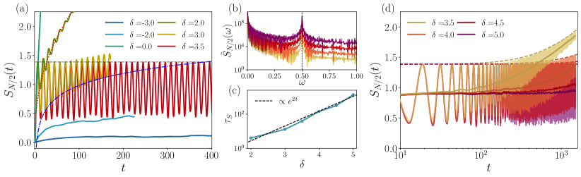
The entanglement dynamics, presented in Figure 3(a), show three clearly distinct behaviors in the different phases of the model. In the MBL paramagnetic phase () the entanglement entropy grows logarithmically in time, as expected for strongly disordered interacting systems [49, 40]. As approaches zero, the system enters the ergodic regime, where entanglement grows as a power law, limiting our numerical simulations. Increasing further, the MBL spin-glass regime sets in, where entanglement shows clear oscillatory behavior. These oscillations eventually flatten out, as one can observe for , and make way to a more standard entanglement growth.
Similarly to the local magnetization case, we use the approximate time-evolution operator, Eq. (2), to explain the main features observed in this regime. Following Ref. [41], we write as a bond dimension matrix-product-operator (MPO), whose entries oscillate at a frequency [45]. While depends on the disorder realization and averages out, the main frequency is common to all realizations and governs the oscillations observed in Fig. 3(a). We further confirm this in Figure 3(b) by comparing the Fourier transform of the entanglement entropy with the analytical expression . The numerical results clearly show a well defined peak at the predicted value, marked by a black dashed line. As in the MBL spin-glass phase we fix , the position of the peak does not depend on .
The small bond dimension of the MPO representation of the time-propagator limits the growth of entanglement entropy to . This is clearly visible in the numerical results shown in Figure 3(a), where the curves at remain below this value (dashed gray line) up to a time increasing with . The growth of above is due to an increase in the bond dimension of the MPO representation of , and therefore to the breakdown of the approximation neglecting the perturbative part of the Hamiltonian . Inspired by Fermi’s golden rule, we use the square of the perturbation strength to estimate the timescale at which its effects become relevant, . Figure 3(c) compares this result to obtained numerically, revealing an accurate agreement.
Beyond this timescale, entanglement starts increasing. While for low values of this growth corresponds to a power law in time (e.g. the red dotted curve for ), at higher disorders the behavior is in line with predictions for bond disordered MBL. In particular, we notice that the lower envelope of the oscillation grows logarithmically in time (blue dotted curve), while the upper one is well captured by , as shown by the dashed lines in panel (d). This suggests that the time-averaged entanglement entropy [solid lines in panel (d)] grows as . Although the timescales we are able to reach are too short to determine the power accurately and we cannot exclude a more standard logarithmic growth (), this behavior agrees with the RG studies of the dynamics in the spin-1/2 XXZ model with bond disorder [43].
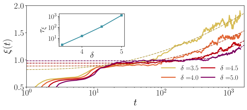
Correlation length.— To additionally characterize the fate of the MBL spin-glass regime, we investigate the behavior of the spin-spin correlation function averaged over disorder realizations, . We observe that the averaged correlation function decays exponentially with distance, , defining a time-dependent correlation length . By fitting the correlation function of the central spin, , to an exponential decay with distance , we extract the time-dependent correlation length and examine its evolution for different values of (see [45] for fit examples).
We distinguish two different behaviors of the correlation length, happening on distinct timescales. At short times, the correlation length rapidly grows and reaches a plateau at . However, on longer timescales the correlation length resumes its growth. Inspired by the entanglement dynamics, we fit this growth to
| (5) |
corresponding to the dashed curves in Fig. 4, and find good agreement with the numerical data (the behavior of could be also consistent with a power-law increase in time, see [45]).
From the fit, we extract , and observe it grows exponentially with , indicating an exponentially long plateau at . It is instructive to compare this timescale to the time that governs the onset of entanglement growth beyond oscillations. As we show in the supplementary [45], the entanglement timescale features a parametrically slower increase with , suggesting that at large disorders entanglement starts growing on top of the oscillations and only at a much later time the correlation length increases.
Discussion – We studied the dynamics from random product states in the MBL-SG phase, revealing characteristic short-time oscillations explained analytically. Over longer timescales, TEBD simulations reveal the emergence of longer-range correlations witnessed by entanglement and spin-spin correlation functions. Understanding the timescales of their growth, and describing them quantitatively, remains an interesting theoretical problem.
More broadly, the slow growth of entanglement we observe is qualitatively consistent with the dynamical RG treatment constructed for a different spin-1/2 model and a specific Neél initial state [43]. Although our analytical results can serve as a starting point for extending the dynamical RG of Ref. [43] to our model, this remains an open question for future work. Our work shows that phenomenological signatures of an infinite randomness fixed point can be detected in quench dynamics. Extending these to the direct observation of clusters of decimated spins as inert degrees of freedom entangled among themselves but decoupled from the rest of the system, and of their hierarchical structure is a fascinating direction for further work. Finally, our results show that the MBL-SG phase can also be dynamically probed in quantum simulation platforms, since non-trivial dynamics arise at sufficiently early times.
Acknowledgements.
Acknowledgments – We thank D. A. Abanin for insightful discussions in the early stages of this work. P. B. acknowledges support by the Austrian Science Fund (FWF) (Grant Agreement No. 10.55776/ESP9057324). The authors acknowledge support by the European Research Council (ERC) under the European Union’s Horizon 2020 research and innovation program (Grant Agreement No. 850899). M. L. acknowledges support by the Deutsche Forschungsgemeinschaft (DFG, German Research Foundation) under Germany’s Excellence Strategy – EXC-2111 – 390814868. The Authors acknowledge PRACE for awarding access to Joliot-Curie at GENCI@CEA, France, where the TEBD simulations were performed. The TEBD simulations were performed using the ITensor library [50].References
- Rigol et al. [2007] M. Rigol, V. Dunjko, V. Yurovsky, and M. Olshanii, Relaxation in a completely integrable many-body quantum system: An ab initio study of the dynamics of the highly excited states of 1d lattice hard-core bosons, Phys. Rev. Lett. 98, 050405 (2007).
- Rigol et al. [2008] M. Rigol, V. Dunjko, and M. Olshanii, Thermalization and its mechanism for generic isolated quantum systems, Nature 452, 854 (2008).
- Rigol [2009] M. Rigol, Breakdown of thermalization in finite one-dimensional systems, Phys. Rev. Lett. 103, 100403 (2009).
- Fagotti et al. [2014] M. Fagotti, M. Collura, F. H. L. Essler, and P. Calabrese, Relaxation after quantum quenches in the spin- Heisenberg XXZ chain, Phys. Rev. B 89, 125101 (2014).
- Essler and Fagotti [2016] F. H. L. Essler and M. Fagotti, Quench dynamics and relaxation in isolated integrable quantum spin chains, J. Stat. Mech.: Theory Exp. 2016 (6), 064002.
- D’Alessio et al. [2016] L. D’Alessio, Y. Kafri, A. Polkovnikov, and M. Rigol, From quantum chaos and eigenstate thermalization to statistical mechanics and thermodynamics, Adv. Phys. 65, 239 (2016).
- Kinoshita et al. [2006] T. Kinoshita, T. Wenger, and D. S. Wiess, A quantum Newton’s cradle, Nature 440, 900 (2006).
- Bloch et al. [2008] I. Bloch, J. Dalibard, and W. Zwerger, Many-body physics with ultracold gases, Rev. Mod. Phys. 80, 885 (2008).
- Trotzky et al. [2012] S. Trotzky, Y.-A. Chen, A. Flesch, I. P. McCulloch, U. Schollwöck, J. Eisert, and I. Bloch, Probing the relaxation towards equilibrium in an isolated strongly correlated one-dimensional Bose gas, Nat. Phys. 8, 325 (2012).
- Gring et al. [2012] M. Gring, M. Kuhnert, T. Langen, T. Kitagawa, B. Rauer, M. Schreitl, I. Mazets, D. A. Smith, E. Demler, and J. Schmiedmayer, Relaxation and prethermalization in an isolated quantum system, Science 337, 1318 (2012).
- Schneider et al. [2012] U. Schneider, L. Hackermüller, J. P. Ronzheimer, S. Will, S. Braun, T. Best, I. Bloch, E. Demler, S. Mandt, D. Rasch, and A. Rosch, Fermionic transport and out-of-equilibrium dynamics in a homogeneous Hubbard model with ultracold atoms, Nat. Phys. 8, 213 (2012).
- Meinert et al. [2013] F. Meinert, M. J. Mark, E. Kirilov, K. Lauber, P. Weinmann, A. J. Daley, and H.-C. Nägerl, Quantum quench in an atomic one-dimensional Ising chain, Phys. Rev. Lett. 111, 053003 (2013).
- Bernien et al. [2017] H. Bernien, S. Schwartz, A. Keesling, H. Levine, A. Omran, H. Pichler, S. Choi, A. S. Zibrov, M. Endres, M. Greiner, V. Vuletić, and M. D. Lukin, Probing many-body dynamics on a 51-atom quantum simulator, Nature 551, 579 (2017).
- Deutsch [1991] J. M. Deutsch, Quantum statistical mechanics in a closed system, Phys. Rev. A 43, 2046 (1991).
- Srednicki [1994] M. Srednicki, Chaos and quantum thermalization, Phys. Rev. E 50, 888 (1994).
- Sutherland [2004] B. Sutherland, Beautiful models: 70 years of exactly solved quantum many-body problems (World Scientific, 2004).
- Basko et al. [2006] D. M. Basko, I. L. Aleiner, and B. L. Altshuler, Metal-insulator transition in a weakly interacting many-electron system with localized single-particle states, Annals of Physics 321, 1126 (2006).
- Gornyi et al. [2005] I. V. Gornyi, A. D. Mirlin, and D. G. Polyakov, Interacting electrons in disordered wires: Anderson localization and low- transport, Phys. Rev. Lett. 95, 206603 (2005).
- Nandkishore and Huse [2015] R. Nandkishore and D. A. Huse, Many-body localization and thermalization in quantum statistical mechanics, Annu. Rev. Condens. Matter Phys. 6, 15 (2015).
- Abanin et al. [2019] D. A. Abanin, E. Altman, I. Bloch, and M. Serbyn, Colloquium: Many-body localization, thermalization, and entanglement, Rev. Mod. Phys. 91, 021001 (2019).
- Sierant et al. [2024] P. Sierant, M. Lewenstein, A. Scardicchio, L. Vidmar, and J. Zakrzewski, Many-body localization in the age of classical computing, Rep. Prog. Phys. 88, 026502 (2024).
- Schreiber et al. [2015] M. Schreiber, S. S. Hodgman, P. Bordia, H. P. Lüschen, M. H. Fischer, R. Vosk, E. Altman, U. Schneider, and I. Bloch, Observation of many-body localization of interacting fermions in a quasirandom optical lattice, Science 349, 842 (2015).
- yoon Choi et al. [2016] J. yoon Choi, S. Hild, J. Zeiher, P. Schauß, A. Rubio-Abadal, T. Yefsah, V. Khemani, D. A. Huse, I. Bloch, and C. Gross, Exploring the many-body localization transition in two dimensions, Science 352, 1547 (2016).
- Lüschen et al. [2017] H. P. Lüschen, P. Bordia, S. Scherg, F. Alet, E. Altman, U. Schneider, and I. Bloch, Observation of slow dynamics near the many-body localization transition in one-dimensional quasiperiodic systems, Phys. Rev. Lett. 119, 260401 (2017).
- Lukin et al. [2019] A. Lukin, M. Rispoli, R. Schittko, M. E. Tai, A. M. Kaufman, S. Choi, V. Khemani, J. Léonard, and M. Greiner, Probing entanglement in a many-body–localized system, Science 364, 256 (2019).
- Guo et al. [2021] Q. Guo, C. Cheng, Z.-H. Sun, Z. Song, H. Li, Z. Wang, W. Ren, H. Dong, D. Zheng, Y.-R. Zhang, R. Mondaini, H. Fan, and H. Wang, Observation of energy-resolved many-body localization, Nat. Phys. 17, 234 (2021).
- Kjäll et al. [2014] J. A. Kjäll, J. H. Bardarson, and F. Pollmann, Many-body localization in a disordered quantum Ising chain, Phys. Rev. Lett. 113, 107204 (2014).
- Moudgalya et al. [2020] S. Moudgalya, D. A. Huse, and V. Khemani, Perturbative instability towards delocalization at phase transitions between MBL phases, arXiv e-prints (2020), arXiv:2008.09113 [cond-mat.dis-nn] .
- Sahay et al. [2021] R. Sahay, F. Machado, B. Ye, C. R. Laumann, and N. Y. Yao, Emergent ergodicity at the transition between many-body localized phases, Phys. Rev. Lett. 126, 100604 (2021).
- Laflorencie et al. [2022] N. Laflorencie, G. Lemarié, and N. Macé, Topological order in random interacting Ising-Majorana chains stabilized by many-body localization, Phys. Rev. Research 4, L032016 (2022).
- Wahl et al. [2022] T. B. Wahl, F. Venn, and B. Béri, Local integrals of motion detection of localization-protected topological order, Phys. Rev. B 105, 144205 (2022).
- Orito et al. [2022] T. Orito, Y. Kuno, and I. Ichinose, Quantum information spreading in random spin chains with topological order, Phys. Rev. B 106, 104204 (2022).
- Chepiga and Laflorencie [2023] N. Chepiga and N. Laflorencie, Topological and quantum critical properties of the interacting Majorana chain model, SciPost Phys. 14, 152 (2023).
- Venn et al. [2024] F. Venn, T. B. Wahl, and B. Béri, Many-body-localization protection of eigenstate topological order in two dimensions, Phys. Rev. B 110, 165150 (2024).
- Chepiga and Laflorencie [2024] N. Chepiga and N. Laflorencie, Resilient infinite randomness criticality for a disordered chain of interacting Majorana fermions, Phys. Rev. Lett. 132, 056502 (2024).
- Huse et al. [2013] D. A. Huse, R. Nandkishore, V. Oganesyan, A. Pal, and S. L. Sondhi, Localization-protected quantum order, Phys. Rev. B 88, 014206 (2013).
- Serbyn et al. [2013] M. Serbyn, Z. Papić, and D. A. Abanin, Local conservation laws and the structure of the many-body localized states, Phys. Rev. Lett. 111, 127201 (2013).
- Bauer and Nayak [2013] B. Bauer and C. Nayak, Area laws in a many-body localized state and its implications for topological order, J. Stat. Mech.: Theory Exp. 2013 (09), P09005.
- Oganesyan and Huse [2007] V. Oganesyan and D. A. Huse, Localization of interacting fermions at high temperature, Phys. Rev. B 75, 155111 (2007).
- Bardarson et al. [2012] J. H. Bardarson, F. Pollmann, and J. E. Moore, Unbounded growth of entanglement in models of many-body localization, Phys. Rev. Lett. 109, 017202 (2012).
- De Nicola et al. [2021] S. De Nicola, A. A. Michailidis, and M. Serbyn, Entanglement view of dynamical quantum phase transitions, Phys. Rev. Lett. 126, 040602 (2021).
- Gross and Bloch [2017] C. Gross and I. Bloch, Quantum simulations with ultracold atoms in optical lattices, Science 357, 995 (2017).
- Vosk and Altman [2013] R. Vosk and E. Altman, Many-body localization in one dimension as a dynamical renormalization group fixed point, Phys. Rev. Lett. 110, 067204 (2013).
- Aramthottil et al. [2024] A. S. Aramthottil, P. Sierant, M. Lewenstein, and J. Zakrzewski, Phenomenology of many-body localization in bond-disordered spin chains, Phys. Rev. Lett. 133, 196302 (2024).
- [45] See suplemental material for derivation of the local magnetization dynamics, for details on the MPO describing the time propagation, for a discussion of the timescales and , and for an analysis of the convergence of the numerical simulations.
- Vidal [2003] G. Vidal, Efficient classical simulation of slightly entangled quantum computations, Phys. Rev. Lett. 91, 147902 (2003).
- Calabrese and Cardy [2005] P. Calabrese and J. Cardy, Evolution of entanglement entropy in one-dimensional systems, J. Stat. Mech.: Theory Exp. 2005 (04), P04010.
- Kim and Huse [2013] H. Kim and D. A. Huse, Ballistic spreading of entanglement in a diffusive nonintegrable system, Phys. Rev. Lett. 111, 127205 (2013).
- Žnidarič et al. [2008] M. Žnidarič, T. Prosen, and P. Prelovšek, Many-body localization in the Heisenberg magnet in a random field, Phys. Rev. B 77, 064426 (2008).
- Fishman et al. [2022] M. Fishman, S. R. White, and E. M. Stoudenmire, The ITensor Software Library for Tensor Network Calculations, SciPost Phys. Codebases , 4 (2022).
- Crosswhite and Bacon [2008] G. M. Crosswhite and D. Bacon, Finite automata for caching in matrix product algorithms, Phys. Rev. A 78, 012356 (2008).
Supplementary Material for “Probing the many-body localized spin-glass phase through quench dynamics”
Pietro Brighi1, Marko Ljubotina2,3,4 and Maksym Serbyn2
Faculty of Physics, University of Vienna, Boltzmanngasse 5, 1090 Vienna, Austria
Institute of Science and Technology Austria, am Campus 1, 3400 Klosterneuburg, Austria
Technical University of Munich, TUM School of Natural Sciences, Physics Department, 85748 Garching, Germany
Munich Center for Quantum Science and Technology (MCQST), Schellingstr. 4, München 80799, Germany
Appendix A Local magnetization dynamics
Here, we evaluate the time-evolution of local magnetization deep in the spin-glass phase . For this purpose, we approximate the Hamiltonian neglecting the terms along the direction. This is well motivated up to timescales , when the effects of the terms along become relevant to the dynamics. The evolution of the local magnetization is given by
| (S1) |
Now, as , one can rewrite the exponentials in the equation above as a sum of sines and cosines
| (S2) |
Since is a product state in the basis, all terms involving Pauli matrices acting on different sites on the left and on the right of identically vanish. Therefore, one remains with
| (S3) |
which is Eq. (3) in the main text.
The analytical expression above further allows for exact disorder averaging of the magnetization dynamics. As each disorder realization introduces an independent set of frequencies, determined by the random couplings , the exact disorder average can be obtained by integrating Eq. (S3) over the distribution function generating the random variables. In the case of a box distribution with unit weight studied here, that corresponds to the characteristic function of the interval , with in the spin-glass phase. The average magnetization can be then obtained as
| (S4) |
corresponding to Eq. (4) in the main text.
Appendix B MPO expression for the time propagator
Deep in the spin-glass phase , the time propagator has a particularly simple structure, which allows us to write it as a low bond dimension matrix product operator (MPO), as mentioned in the main text. Here, we show how the MPO is obtained.
The Hamiltonian Eq. (1) can be written separating terms diagonal in the and bases
| (S5) |
In the spin-glass phase , and we can approximate . Since all terms in the Hamiltonian commute with one another we can write the time propagator as a product of local operators acting on three sites: , with . Each local term in the product is diagonal in the basis, with its coefficients determined by the state of the two spins to its left.
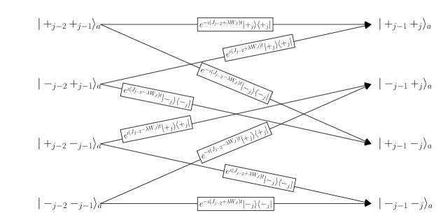
One can conveniently write the time propagator as a bond dimension MPO with
| (S6) |
As mentioned above, at each site the sign of the coefficients in the exponential is determined by the state of the two spins to the left of . Therefore, the auxiliary dimension of the MPO has to encode the information on the two sites to the left, thus leading to corresponding of the possible states of and in the basis, in which the operators are diagonal. A schematic automaton picture [51] of the MPO is represented in Figure S1.
The explicit construction of the MPO defining the time evolution is useful in obtaining relevant features of the entanglement entropy. First, as has a finite bond dimension the entanglement entropy cannot exceed , as shown in the main text. Furthermore, from the analysis of the exponent we notice that there are two terms contributing to the dynamics: a random frequency which is different on each site and in all disorder realizations, and a fixed frequency independent of site, disorder realization and disorder strength since as . In the average entanglement dynamics, then, the random contributions will typically average out, leaving a single dominant frequency for the oscillations at . Both these predictions are confirmed by comparison with numerical simulations shown in the main text.
Appendix C Examples of correlation function exponential fit and power law fit for
In the main text we defined the corelation length as the length scale for the exponential decay of the disorder averaged correlation function . We notice that for our particular choice of initial state and therefore the connected part of the correlation function coincides with . In an infinite system, the disorder averaged correlation length is expected to be the same on all sites, as each local disorder is independently drawn. However, as we deal with finite systems, we chose to study the decay of the correlation function from the central spin to reduce the finite size effects. This defines the correlation length shown in the main text, which upon sufficient disorder averaging coincides with the generic correlation length .
In this Section, we show numerical data confirming the exponential decay of the disorder averaged correlation function, as shown in Figure S2 (a). Our numerical simulations show a clear exponential behavior (modulo small oscillations due to finite disorder average) in good agreement with the fit (dashed lines). The data are shown for a single arbitrary time , but do not change qualitatively for different choices of .
The correlation length was fitted in the main part to the square logarithmic behavior predicted for the entanglement entropy by renormalization group analysis [43]. However, the range of growth of the correlation is too limited to uniquely determine its functional behavior. Here, we report an alternative power law fit, whose precision is comparable to the one used in the main text (although it is not supported by any theoretical argument). In Figure S2 (b) we show the correlation length dynamics for all the values of within the MBL-SG phase together with a power law fit (dashed lines). The algebraic growth is similar for all values of , with a coefficient decaying with . Both the power law and the logarithmic behavior shown in the main text define a timescale for the growth of the correlation length beyond growing exponentially with . In Figure S2 (c) we compare this timescale as obtained from Eq. (5) with the analogue obtained for entanglement growth. Remarkably, the two have different scaling with , with increasing more slowly than . While asymptotically then entanglement would start growing earlier than correlations, within this range of parameters , thus implying a faster growth of the correlation length as compared with entanglement entropy.
Appendix D Bond dimension analysis
In this Section we present the bond dimension analysis of our tensor network simulations. In particular, we focus on the spin-glass region of the parameter space, , which is the central topic of the main part of the text.
In matrix product states (MPS), as the wavefunction gets decomposed in order- tensors, one defines a truncation value such that all singular values are neglected, and a maximum bond dimension corresponding to the maximum number of singular values that can be stored per bond. Therefore, to ensure the accuracy of numerical results, one needs to check the convergence in either of these parameters.
In Figure S3, we compare the observables studied in the main text. In panels (a) and (b), we show local magnetization and entanglement entropy in the center of the chain at and for two values of bond dimension . The curves corresponding to the two different bond dimensions perfectly overlap, thus ensuring convergence of our numerical simulations. In panel (c), instead, we show the behavior of the correlation function for two different values of the truncation threshold at fixed and at time . As this bond dimension never gets saturated at these values of (i.e. the number of singular values is smaller than ), it is worth comparing two different truncation thresholds, especially for a quantity like the correlation function, where we care about its exponential decay. As the figure shows, the curves overlap perfectly up to values , thus again ensuring the reliability of our data.