Latest Advancements Towards Catastrophic Forgetting under Data Scarcity: A Comprehensive Survey on Few-Shot Class Incremental Learning

Abstract

Data scarcity significantly complicates the continual learning problem, i.e., how a deep neural network learns in dynamic environments with very few samples. However, the latest progress of few-shot class incremental learning (FSCIL) methods and related studies show insightful knowledge on how to tackle the problem. This paper presents a comprehensive survey on FSCIL that highlights several important aspects i.e. comprehensive and formal objectives of FSCIL approaches, the importance of prototype rectifications, the new learning paradigms based on pre-trained model and language-guided mechanism, the deeper analysis of FSCIL performance metrics and evaluation, and the practical contexts of FSCIL in various areas. Our extensive discussion presents the open challenges, potential solutions, and future directions of FSCIL.

1 Introduction

The few-shot class incremental learning (FSCIL) problem simulates a real-world problem where a machine learning model is deployed to learn dynamic environments with very few samples Tao et al. (2020). FSCIL problem is broadly applied in various area e.g. medicalSun et al. (2024b), remote sensingZhao et al. (2022), audio processingWang et al. (2021), and data mining Tan et al. (2022). The presence of the data scarcity constraint in FSCIL hardens the catastrophic forgetting problem to be solved. As a clear proof, rehearsal-based class incremental learning (CIL) methods Boschini et al. (2022), and event joint-training mechanism fail to overcome the FSCIL problem. Thus, it calls for advanced solutions beyond CIL methods. On the other sides, popular rehearsal-based methods in the CIL problem cannot be applied in the FSCIL problem because it might result in all samples to be stored in the memory.

In the earlier stages, various FSCIL methods have been developed, offering different approaches i.e. backbone tuning Shi et al. (2021), meta-learning Chi et al. (2022), prototype-tuning Chen and Lee (2021), and dynamic network approach Zhang et al. (2021). Most of the methods fully train the backbone parameters in the base task, then train a small subset of the backbone or part of the model e.g. projection and weighting in the few-shot tasks. This implies that the model relies too much on the base task performance. In addition, the model barely achieves plasticity in the new tasks, while suffering from a high risk of forgetting on the base task.

Meanwhile, the use of the foundation model and the parameter-efficient fine-tuning (PEFT) approach offer a breakthrough solution to the catastrophic forgetting problem Wang et al. (2022c). The pre-trained model that has strong background knowledge handles the dependency on the base task. In addition, the approach offers far smaller learnable parameters than the previous approaches and reduces the model training time by a large margin. The second advancement is the language-guided learning approach pioneered by Khan et al. (2023) that contributes to the advancement of the FSCIL method. Language-guided learning offers discriminative representations through encoded text embedding of respective classes by a pre-trained vision-language model (VLM) such as CLIPRadford et al. (2021). That is, the use of language modality alleviates the data scarcity problem because it offers complementary information of those input images.

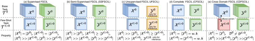
Figure 1: Types of FSCIL settings and their properties (a) Fully-Supervised, (b) Semi-Supervised (c) Unsupervised (d) Complete (e) Cross-Domain FSCIL

The recent survey Tian et al. (2024) systematically discussed the four approaches of FSCIL methods from the theoretical perspective and application. However, the survey doesn’t cover the latest advancement of the PEFT approach and language-guided learning of FSCIL. Second, the survey also doesn’t yet cover the important advancements of FSCIL settings i.e. semi-supervised (SSFCIL)Cui et al. (2021), unsupervised (UFSCIL)Ma’Sum et al. (2024b), complete (CFSCIL)Lin et al. (2024) and cross-domain (CDFSCIL)Yang et al. (2023a) that have been applied in various research areas. Third, prototype bias and rectificationLiu et al. (2020) that are the important aspects of data scarcity haven’t been discussed yet in the survey. Last but not least, the subtle details such as backbone and parameters, details of base classes, and novel classes performance i.e., stability-plasticity performance haven’t been discussed as well. These intriguing factors motivate us to write a comprehensive survey on FSCIL. We offer a comprehensive FSCIL (sub-)settings, detailed topology, and formal objectives of each FSCIL approach, broad yet detailed aspects in FSCIL methods comparison, accommodating the latest advancement of FSCIL. Then, we present the open problem, potential solution and future direction of FSCIL. Specifically, our contributions are summed up:

• We propose a comprehensive FSCIL topology highlighting the latest advancement of FSCIL methods, especially the new PEFT approach, the formal objective of each approach, and sub-settings of FSCIL i.e. SSFSCIL, UFSCIL, CFSCIL, and CDFSCIL.

• We analyze broader aspects of FSCIL methods i.e. backbone type, learnable parameters, classifiers, the use of the pre-trained model (PTM), augmentation, general performance and stability-plasticity performance detailed in base classes, and novel classes performance.

• We highlight the importance of prototype rectification to handle prototype bias due to data scarcity issues in the few-shot tasks. We classify the rectification mechanisms into a topology for a better understanding.

• We present a rigorous analysis of the current open problem, potential solution, and future direction of FSCIL related to applicable real-world constraints i.e. data privacy, data streams, and open-world problem.

2 Preliminaries

2.1 Problem Formulation

Few-Shot Class-Incremental Learning (FSCIL) is defined as: Given a sequence of tasks $[0,1,2,...,T]$ where each task $t$ carries a labeled training set $\mathcal{T}^{t}=\{(x_{i}^{t},y_{i}^{t})\}_{i=1}^{|\mathcal{T}^{t}|}$, where $x_{i}^{t}\in\mathcal{X}^{t}$ denotes an input image and $y_{i}^{t}\in\mathcal{Y}^{t}$ denotes its label, and $|.|$ denotes the cardinality. Each task $t$ is disjoint with another task $t^{\prime}$. i.e. $\forall_{t,t^{\prime}}\mathcal{T}^{t}\cap\mathcal{T}^{t^{\prime}}=\emptyset$. The first task $(t=0)$ carries abundant training samples while the remaining tasks $(t>0)$ carries only far smaller samples than the first task i.e $|\mathcal{T}^{0}|>>|\mathcal{T}^{t>0}|$. For a convenient way, task-$0$ is called the base task while the rest is called the few-shot task (FS task). Let a deep neural network $g_{\phi}(f_{\theta}(.))$ be parameterized by $\theta$ and $\phi$ where $f(.)$ and $g(.)$ are the feature extractor and classifier respectively. The objective of FSCIL is to achieve the optimum parameters ${\theta*}$ and ${\phi*}$ so that $g_{\phi*}(f_{\theta*}(.))$ recognizes all the learned classes from the first task until the current task $t$ i.e. $\{\mathcal{T}^{0},...,\mathcal{T}^{t}\}$. Formally, FSCIL objective is defined as in equation 1.

$$\small\theta*,\phi*=\operatorname*{arg\,min}_{\theta,\phi}\mathbf{E}_{(x,y)\in\mathcal{T}^{0}\cup\mathcal{T}^{1}...\mathcal{T}^{t}}\mathbf{I}(y=g_{\phi}(f_{\theta}(x)))$$ (1)

where $\mathbf{E}$ denotes the expectation, $\mathbf{I}$ denotes the binary function that outputs 1 if the condition is met and 0 otherwise.

2.2 Types of FSCIL Setings

There are 3 types of FSCIL setting based on the training mechanism with respect to the number of images and labels, i.e. $|\mathcal{X}|$ and $|\mathcal{Y}|$ as follows:

a). Supervised FSCIL or just FSCIL Tao et al. (2020) utilizes the fully supervised training mechanism that is conducted in the case where the number of images and labels are the same for every task, i.e. $|\mathcal{X}^{t}|=|\mathcal{Y}^{t}|$ for all $t\in[1,2..T]$. In the few-shot task ($t>0$), the number of images and labels are the same and equal to the $k$-shot value.

b). Semi-Supervised FSCIL (SSFSCIL)Cui et al. (2021) deploys supervised and unsupervised training mechanisms in the case where the number of images is greater than the number of labels, i.e. $|\mathcal{X}^{t}|>|\mathcal{Y}^{t}|$ for any $t\in[1,2..T]$. The semi-supervised training is not necessarily conducted in all tasks, it can be conducted only in the base task where abundant samples are available but only fewer labels are provided.

c). Unsupervised FSCIL (UFSCIL)Ma’Sum et al. (2024b) deploys only unsupervised training mechanisms to deal with the unavailability of training label i.e. $|\mathcal{Y}^{t}|=0$ for all $t\in[1,2..T]$. A small fraction of labels are available i.e. $|\mathcal{Y}^{t}|<<|\mathcal{X}^{t}|$ only for inference purpose since the model needs to give predicted label for any input $x$.

d). Complete FSCIL (CFSCIL)Hersche et al. (2022) remove the assumption that the base task has abundant labeled samples. Thus, all task only hold a few labeled samples and organized in n-way k-shot setting i.e. $|\mathcal{X}^{t}|=|\mathcal{Y}^{t}|=w.k$ for all $t\in[1,2..T]$, where $w$ is the number of classes in each task, and $k$ is the number of samples (shot) for each class.

e). Cross Domain FSCIL (CDFSCIL)Hersche et al. (2022) is similar to supervised FSCIL, but assumes that few-shot task and base task have different domains i.e. $\mathcal{D}^{0}\neq\mathcal{D}^{t>0}$. The illustration and property of all settings is visualized in fig.1.

3 FSCIL Approaches

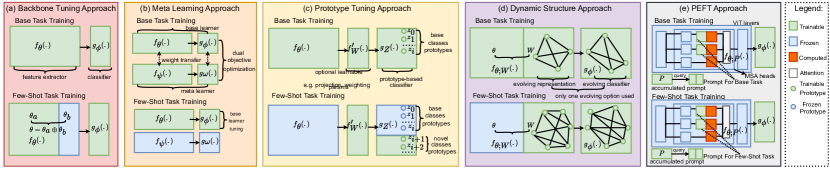
Figure 2: Visualization of FSCIL Approaches i.e. (a) backbone tuning approach, (b) meta learning approach, (c) prototype tuning approach, (d) dynamic structure approach, and (e) parameter efficient fine tuning (PEFT) approach.

3.1 Backbone Tuning Approach

The backbone tuning approach trains the whole backbone and classifier parameters in the base task, then trains the classifier and some of backbone parameters in the few-shot tasks as illustrated in fig. 2 (a). Suppose that $\theta=\theta_{a}\oplus\theta_{b}$, where $\theta_{a}$ and $\theta_{b}$ are front part (earlier layers) and back part (latest layers) of the feature extractor parameters, and $\oplus$ denotes concatenation. In the base task, the method optimizes $\theta$ and $\phi$, while in the few-shot tasks, the method freezes $\theta_{a}$ and optimizes $\theta_{b}$ and $\phi$. In general, the objective of backbone tuning approach is defined as in equation 2.

$$\small\begin{split}\theta*,\phi*=\operatorname*{arg\,min}_{\theta,\phi}\mathbf{E}_{(x,y)\in\mathcal{T}^{0}}\mathbf{I}(y=g_{\phi}(f_{\theta}(x)))\text{ if }(t=0)\\ \theta_{b}*,\phi*=\operatorname*{arg\,min}_{\theta_{b},\phi}\mathbf{E}_{(x,y)\in\mathcal{T}^{0}\cup...\mathcal{T}^{t}}\mathbf{I}(y=g_{\phi}(f_{\theta}(x)))\text{ else }\end{split}$$ (2)

Several strategies are enforced in this aproaches i.e. GPTree Achituve et al. (2021) utilizes Gaussian Process to approximate the distribution of classes with few-shot labeled samples. Similarly, LDCLiu et al. (2023) enforces a learnable models to approximate the distribution. F2MShi et al. (2021) and FLOWERMa’sum et al. (2024a) create a flat loss region by perturbating latest part of the backbone parameters i.e. $\mathcal{L}((x,y);\theta_{a}\oplus(\theta_{b}+\epsilon);\phi))$ is minimal for any $-b\leq\epsilon\leq b$, where $\epsilon$ and $b$ is perturbation noise and bound respectively. ERDRLiu et al. (2022) and Akyürek et al. (2022) utilize customized regularization strategy i.e. entropy and subspace regularization respectively. FeSSSAhmad et al. (2022) utilizes self-supervised method and feature fusion to obtain more discrimivative features. Mixed-up features are also utilized by M2SDLin et al. (2024) and combined with mixed-up distillations. SoftNetKang et al. (2022) adds binary mask $m$ and gating function to sub-network of $\theta$. It enables different weight of $\theta$ for different samples. On the other hand, WaRPKim et al. (2023) transforms sub-net of $\theta$ with multiple axis rotation to gain distinctive representations.

3.2 Meta-Learning Approach

Inspired from MAMLFinn et al. (2017) meta learning approach (fig. 2 (b)) trains both meta learner and base learner with the different sets of data i.e. training and validation set. Validation set can be obtained from auxiliary (open) dataset or by transforming the training set with sequence of operations. Suppose that $f_{\psi}(.)$ is the meta learner parametrized by $\psi$, and $\mathcal{T}_{v}^{t}=\text{ Transform}(\mathcal{T}^{t})$ is validation set transformed from $\mathcal{T}^{t}$. then the dual objective of meta learning-based FSCIL is formulated in eq. 3.

$$\small\begin{split}\psi*=\operatorname*{arg\,min}_{\psi}\mathbf{E}_{(x,y)\in\mathcal{T}_{v}^{0}\cup...\mathcal{T}_{v}^{t}}\mathcal{L}(f_{\psi}(x))\\ \text{s.t. }\theta*,\phi*=\operatorname*{arg\,min}_{\theta,\phi}\mathbf{E}_{(x,y)\in\mathcal{T}^{0}\cup...\mathcal{T}^{t}}\mathbf{I}(y=g_{\phi}(f_{\theta}(x)))\end{split}$$ (3)

MetaFSCILChi et al. (2022) utilizes bidirectional guided modulation (BGM) that allows meta and base learners to map their weights one to another. C-FSCILHersche et al. (2022) utilize meta learning to perform 3 modes of prototypes training i.e. averaged prototypes, retraining on bipolarized-prototypes, and retraining on nudged-prototypes. Both MetaFSCIL and C-FSCIL train meta learner only in the base task, it is frozen afterwards. XTarNetYoon et al. (2020) deploys CNN as meta learner, utilizes a pretrained backbone, and adds two additional modules i.e. MergeNet and TConNet that performs weights merger and conditioning classifier respectively. Similar mechanism is performed by LIMITZhou et al. (2022b) that utilize meta learning for prototype tuning. LIMIT generates multiple prototypes from an input instance, then the prototypes are calibrated by meta learner then aggregated with inner product into a final prototype.

3.3 Prototype-Tuning Approach

Prototype tuning approach is the most common method in FSCIL due to its simplicity and scalability. Suppose that $z_{c}$ is the prototype of class $c$, $Z^{t}={z^{t}_{c}}$ is the prototype set of task $t$ contains prototypes of any class $c$ exists in $\mathcal{T}^{t}$ , and $Z=Z^{0}\cup Z^{1},...\cup Z^{t}$ is the prototype set of all learned classes from task $0$ to task $t$. The approach utilizes prototype-based classifier $g_{Z}(.)$ instead of standard MLP classifier $g_{\phi}(.)$. Thus it optimizes $Z$ in every task, while feature extractor parameter $\theta$ is optimized only in the base task. A prototype-based method may utilize an additional network $f^{\prime}_{W}(.)$ parameterized by $W$ between backbone $f_{\theta}(.)$ and prototype-based classifier $g_{Z}(.)$ for projection, weighting, or refinement. The objective of the prototype tuning approach is defined in eq. 2.

$$\scriptsize\begin{split}\theta*,W*,Z*=\operatorname*{arg\,min}_{\theta,W,Z}\mathbf{E}_{(x,y)\in\mathcal{T}^{0}}\mathbf{I}(y=g_{Z}(f^{\prime}_{W}(f_{\theta}(x))))\text{ if}(t=0)\\ W*,Z*=\operatorname*{arg\,min}_{Z}\mathbf{E}_{(x,y)\in\mathcal{T}^{0}\cup...\mathcal{T}^{t}}\mathbf{I}(y=g_{Z}(f^{\prime}_{W}(f_{\theta}(x))))\text{ else}\end{split}$$ (4)

IDLVQChen and Lee (2021) optimizes vector $Z$ to directly classify backbone feature $f_{\theta}(x)$. There are several variations to implement $f^{\prime}_{W}(.)$ i.e. dynamic relation projection as in SPRRZhu et al. (2021), subspace projection as in SFMSCheraghian et al. (2021b), orthogonal projection as in ORCOAhmed et al. (2024), merged multiple embeddings by attention as in SAKDCheraghian et al. (2021a), kernel analytics module as in GKEALZhuang et al. (2023), positive-negative weighting matrices as in CLOMZou et al. (2022), compositional weighting as in Comp-FSCILZou et al. (2024), prototype rectification as in TEEN Wang et al. (2024a) and YOURSELFTang et al. (2024) or any customized refinement. Along with prototype tuning, this approach also applies conceptual learning methods e.g. contrastive learning as in SAVCSong et al. (2023), virtual(augmented) prototypes as in FACTZhou et al. (2022a) and ALICEPeng et al. (2022), neural collapse as in NC-FSCILYang et al. (2023b), and Slow-and-Fast learning as in MgSvfZhao et al. (2021).

3.4 Dynamic Architecture Approach

Dynamic architecture approach tackles FSCIL challenges by incrementally evolving its architecture to adapt to the new tasks. Fig. 2 (d) shows that this approach can be implemented into two types of growing component, i.e. growing representation $W$ or growing classifier $\phi$. TOPICTao et al. (2020) grows neural gas $W$, a graph-like structure to obtain a more discriminative class representation. BiDistZhao et al. (2023a) adds learnable weight for each task $W^{t}$ then uses bilateral distillation of current and previous tasks representation. CECZhang et al. (2021) transforms incrementally added linear classifier into graph structure. S3C grows stochastic classifiers by continually adding 4-angles (0,90,180,270) representations. LEC-NetYang et al. (2021) expands learnable compression network $W$ to mitigate overfitting due to data scarcity. Similarly, DSNYang et al. (2022) expands self-activation and compression network. The objective of the dynamic architecture approach is defined in eq. 5.

$$\scriptsize\begin{split}\theta*,W*,\phi*=\operatorname*{arg\,min}_{\theta,W,\phi}\mathbf{E}_{(x,y)\in\mathcal{T}^{0}}\mathbf{I}(y=g_{\phi}(f_{\theta;W}(x)))\text{ if }(t=0)\\ W*,\phi*=\operatorname*{arg\,min}_{W,\phi}\mathbf{E}_{(x,y)\in\mathcal{T}^{0}\cup...\mathcal{T}^{t}}\mathbf{I}(y=g_{\phi}(f_{\theta;W}(x)))\text{ else }\end{split}$$ (5)

3.5 Parameter Efficient Fine Tuning (PEFT) Approach

The PEFT approach proposes a unique new solution for FSCIL by training small-sized parameters (prompts) on top of frozen pre-trained backbone e.g. visual transformer (ViT). Different to CNN, ViT has sequence of layers, where a layer contains Multiples Self Attention (MSA) heads combined with other components, each performing self-attention function as in eq. 6:

$$\small A(Q,K,V)=Softmax((Q.K^{T})/\sqrt{D/h})V$$ (6)

where $Q,K$, and $V$ are query, key, and value vectors obtained by processing an input patch into respective weights i.e. $x.W^{Q},x.W^{K}$, and $x.W^{V}$, $D$ and $h$ denote patch dimension and number of heads respectively. Prompt-based method attaches a small learnable prompts into a frozen pre-trained ViT model (fixed $\psi$) Wang et al. (2022c). The attachment techniques are mainly divided into 2 types i.e. prompt tuning and prefix tuning Li and Liang (2021). Prompt tuning as in L2P Wang et al. (2022c) inserts a prompt vector $P$ into query, key, and value of MSA, then the attention mechanism is computed as $A([P\oplus Q],[P\oplus K],[P\oplus V])$, where $\oplus$ denotes concatenation operation. Prefix tuning as in DualP Wang et al. (2022b) divides $P$ into pair of $P^{K}$ and $P^{V}$ for key and value respectively, then the attention mechanism becomes $A(Q,[P^{K}\oplus K],[P^{V}\oplus V])$. The structure of $P$ can be defined by several options, i.e. pool-based structure as in L2P, task-wise structure as in DualP, growing component structure as in CODA-PSmith et al. (2023), or any customized structure.

ASPLiu et al. (2024) deploys task-aware task-invariant prompts to improve prompt selection during the testing phase. Besides, it utilizes a prompt encoder that produces an additional (second) prompt. Privilege Park et al. (2024) leverages vision and language modalities and prepends concatenation of vision and language prompts. Similarly, FineFMPLSun et al. (2024a) performs language-guided prompting i.e. tuning vision prototype by language prototypes. In addition, it utilizes two types of vision prototypes i.e. global level and object level prototypes. ApproxFSCILWang et al. (2025) concatenates ViT layers with norm layers and tanh function instead of prompt, then bounds training process with transfer risk and consistency risk. Formally, the objectives of PEFT approach is presented in eq.7.

$$\small P*,\phi*=\operatorname*{arg\,min}_{P,\phi}\mathbf{E}_{(x,y)\in\mathcal{T}^{0}\cup...\mathcal{T}^{t}}\mathbf{I}(y=g_{\phi}(f_{\theta;P}(x)))$$ (7)

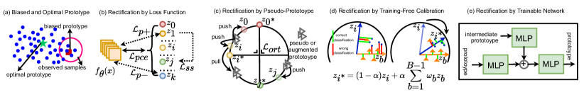
Figure 3: Biased Prototype, Optimal Prototypes, and Types of Prototype Rectification Mechanism (a) Biased and Optimal Prototype (b) Rectification by Loss function only (c) by pseudo-prototypes (d) by training-free calibration (e) by trainable networks

4 Trends and Finding

4.1 Backbone, Parameters, and Pre-trained Model (PTM)

As shown in tab. 1, ResNet18 is the preferred backbone for backbone tuning, meta-learning, prototype-tuning, and dynamic structure approach following the pioneer of FSCIL settingTao et al. (2020). However, the recent advancement of PEFT approach utilized ViT instead of ResNet. This is one of the clear impacts of the advancement of the foundation model. Despite utilizing a bigger backbone i.e. ViT-B/16 with 86M parameters, PEFT approach has the smaller trainable parameter i.e. 0.2-11.9M as all the pre-trained backbone weights are frozen, except YourSelf. YourSelf fine-tunes its backbone in the base classes resulting a bigger trainable parameters, albeit utilizing fewer layers of ViT.

The other 4 approaches have bigger trainable parameters i.e. 11.7-41.7M albeit utilizing the smaller backbone i.e. 11.7M as these approaches tune the whole backbone in the base task. Note that a method usually has more parameters than the backbone and classifiers e.g. projection, weighting, self-attention, or rectifier. Thus, these approaches train more parameters. PEFT utilizes a PTM for all scenarios, while the rest utilizes PTM in the CUB dataset. This fact gives us 2 insights, first, training the backbone from scratch isn’t enough for a dataset with small (30 or fewer) samples per class, and second we can compare all the methods head to head in CUB dataset as all the methods utilize PTM.

4.2 Prototype-based over Network-based Classifiers

The table shows that the prototype-based classifier is highly preferable than the network-based classifier such as MLP or reconstructed linear network Zhang et al. (2021). A prototype-based classifier uses classes’ prototypes where a prototype is optimized only in a particular task. Thus, it won’t be adjusted in the upcoming tasks. Thus, it reduces the risk of forgetting. On the contrary, a network-based classifier is adjusted in each task, thus it has a higher chance of forgetting.

Several methods utilize combined or customized classifiers. GKEAL and Comp-FSCIL utilize a combination of linear and prototype-based classifiers. The methods have a selection mechanism to choose which classifiers will be utilized in the inference phase. PriViLege and FineMPL utilize both vision and language prototypes since the methods adopt language-guided learning. S3C generates multiple prototypes with angular rotation, and then performs a stochastic classification based on the similarity to the prototypes.

4.3 Image vs Feature Augmentation

Several FSCIL methods utilize augmentation to handle data scarcity in FSCIL, aside from standard augmentation such as random crop and random flip, commonly used in a data loader setting. Image augmentation offers a low-level and simple procedure but consumes higher system memory. On the contrary, augmentation in the feature space requires a lower memory size, but it needs more complex operation and validation. For example, image-space augmentation can be validated via a visual plot, while feature-space augmentation should be evaluated by valid metrics such as Euclidean distance, or loss. GP-tree augments its likelihood estimator rather than image or prototype augmentations since it performs a Gaussian process in its training phase. Tab.1 shows that the latest methods don’t perform any augmentations.

4.4 The Importance of Prototype Rectification

As shown in tab.1 all the methods that utilize prototype-based classifiers perform prototype rectification to maximize class discrepancies. As emphasized in Liu et al. (2020), and visualized in fig.3(a) a few observed samples have a high chance of producing a biased prototype i.e. a prototype that only represents the few observed samples but not the whole distribution. Thus a rectification is necessary to adjust the biased prototype into the optimal prototype.

The existing FSCIL methods perform various types of rectification as illustrated in fig.3(b)-(d). The simplest mechanism is rectification by loss where classes’ prototypes are adjusted based on similarity to the input features or between classes prototypes. There are many types of loss that can be utilized to perform this rectification e.g. prototypical-cross-entropy $\mathcal{L}_{pce}$, self-supervised loss $\mathcal{L}_{ss}$, or contrastive loss based on positive and negative prototypes i.e. $\mathcal{L}_{p+}$ and $\mathcal{L}_{p-}$. The second type is rectification by pseudo prototypes. Pseudo-prototypes can be obtained by generating several prototypes from different layers, model perturbations, or augmentation. Some methods like OrCoAhmed et al. (2024) utilize orthogonal loss $\mathcal{L}_{ort}$ to minimize dot product between classes’ prototypes. Rectification by training-free calibration Wang et al. (2024a) adjusts a prototype of novel classes based on weighted similarities to the base classes’ prototypes. While rectification by trainable networks utilizes an extra trainable model to calibrate the prototype Tang et al. (2024). Training-free calibration is less complex than rectification by pseudo-prototypes or trainable networks since it doesn’t need extra operations for generating pseudo-prototypes.

4.5 The Use of Language-Guided Learning

The advancement of the vision-language model (VLM) such as CLIPRadford et al. (2021) drives the utilization of language-guided learning in FSCIL. PriViLegePark et al. (2024) deploys language prototypes along with vision prototypes as loss anchors and classifiers, while FineMPLSun et al. (2024a) merges both prototypes into one long prototype and then uses it for the same purpose. Despite only 2 methods that utilize language-guided learning, the studies show a promising future for the approach.

4.6 Performance

Tab.1 shows the overall performance on 3 main FSCIL benchmark datasets, in terms of average accuracy(AA) from the first until the last task, performance drop (PD) between the first and the last task and average harmonic accuracy (AHM) that represent stability-plasticity balance from the second until the last task. In general, AA in three datasets that is still below 90% shows that FSCIL offers a big opportunity for improvement. The high accuracy ($>$ 90%) in MiniImageNet by Privilege, FineMPL and ApproxFSCIL are common-sense results as the methods utilize pre-trained ViT on ImageNet (the superset of MiniImageNet). The results on the CUB dataset, where the PEFT method achieves relatively higher AA show the impact of the bigger backbone i.e. ViT (86.7M) over ResNet18(11.7M) since all methods utilize PTM. The high magnitude of PD i.e. up to 42% shows that catastrophic forgetting with data scarcity remains a difficult problem.

PEFT methods e.g. ASP and Privilege confirm the superiority of the PEFT approach to the other 4 approaches with a significant gap i.e. up to 20%. The improvement from L2P, DualP, and CodaP to L2P+, DualP+, and CodaP+ confirms the significant impact of the prototype-based classifier for FSCIL methods. The other 4 approaches have competitive performance in those 3 datasets, with similar trends i.e. the latest methods outperform the earlier methods. Both from AA and PD measurement, the best performers of those 4 approaches are below the best performer of the PEFT approach.

			BackBone								Perf. On MiniImageNet			Perf. On CIFAR100			Perf. On CUB
Method	Year	Venue	Type	Size	Learn. Param.	Utilize PTM on	Classifier	Aug	Proto. Rect.	Lang. Guided	AA	PD	AHM	AA	PD	AHM	AA	PD	AHM
GP-Tree	2021	ICML	ResNet18	11.67M	-	CUB	Network	Likelihood	✗	✗	46.68	14.10	-	-	-	-	54.26	30.12	-
FSLL	2021	AAAI	ResNet18	11.67M	-	CUB	Prototype	✗	Loss	✗	52.58	13.90	-	47.59	16.51	-	60.93	18.56	-
F2M	2021	NIPS	ResNet18	11.67M	11.67M	CUB	Prototype	✗	Loss	✗	54.89	12.39	-	53.65	11.06	-	69.49	20.81	-
ERDR	2022	ECCV	ResNet18	11.67M	-	CUB	Network	✗	✗	✗	58.02	13.82	-	60.78	13.62	-	61.52	23.51	-
SubspaceReg.	2022	ICLR	ResNet18	11.67M	26.30M*	-	Network	✗	✗	✗	63.71	16.66	-	-	-	-	-	-	-
FeSSSS	2022	CVPR	ResNet18	11.67M	-	CUB	Prototype	✗	Loss	✗	68.24	13.26	-	-	-	-	62.86	26.62	-
LDC	2023	TPAMI	ResNet18	11.67M	-	CUB	Prototype	Feature	Tr. Net.	✗	63.99	11.83	-	64.35	11.61	-	68.32	16.31	-
SoftNet	2023	ICLR	ResNet18	11.67M	22.38M*	CUB	Prototype	✗	Loss	✗	64.32	13.78	-	65.86	14.14	-	64.74	22.00	-
WaRP	2023	ICLR	ResNet18	11.67M	-	CUB	Network	✗	✗	✗	74.12	9.18	-	74.55	11.65	-	55.86	18.38	-
FLOWER	2024	TNNLS	ResNet18	11.67M	12.25M	CUB	Prototype	Feature	Loss	✗	59.55	15.05	-	59.42	13.98	-	65.67	21.53	-
M2SD	2024	AAAI	ResNet18	11.67M	-	CUB	Network	Image	✗	✗	68.63	13.48	-	68.25	13.55	-	68.24	19.66	-
XtarNet	2021	ICML	Resnet18	11.67M	-	-	Prototype	✗	Loss	✗	66.86	-	-	-	-	-	-	-	-
C-FSCIL	2022	CVPR	ResNet18	11.67M	12.79M*	-	Prototype	✗	Loss	✗	61.61	14.79	29.55	61.64	15.83	25.66	-	-	-
Meta-FSCIL	2022	CVPR	ResNet18	11.67M	-	CUB	Network	✗	✗	✗	58.85	13.19	-	60.79	13.71	-	61.93	23.26	-
LIMIT	2022	TPAMI	ResNet18	11.67M	12.33M	CUB	Prototype	Feature	Loss	✗	59.06	13.26	33.36	61.84	11.97	33.89	66.67	17.87	53.57
SPPR	2021	CVPR	ResNet18	11.67M	12.36M	CUB	Prototype	✗	Loss	✗	52.76	8.69	-	54.52	9.58	-	49.32	31.35	-
IDLVQ	2021	ICLR	ResNet18	11.67M	-	CUB	Prototype	✗	Loss	✗	51.16	13.61	-	54.89	12.39	-	65.23	19.56	-
SAKD	2021	CVPR	ResNet18	11.67M	-	CUB	Prototype	✗	Pse. Proto.	✗	50.86	11.14	-	50.63	10.77	-	46.13	35.27	-
SFMS	2021	ICCV	ResNet18	11.67M	-	CUB	Prototype	Feature	Pse. Proto.	✗	50.77	10.60	-	50.86	11.17	-	51.84	25.55	-
FACT	2022	CVPR	ResNet18	11.67M	11.34M	CUB	Prototype	Feature	Pse. Proto.	✗	60.79	15.51	24.16	63.10	15.40	34.91	64.42	18.96	51.58
ALICE	2022	ECCV	ResNet18	11.67M	41.71M	CUB	Prototype	Image	Loss	✗	63.99	16.61	-	63.21	15.79	-	65.75	17.30	-
MgSvF	2022	TPAMI	ResNet18	11.67M	-	CUB	Prototype	✗	Loss	✗	52.65	10.24	-	61.32	12.74	-	62.37	17.96	-
CLOM	2022	CVPR	ResNet18	11.67M	18.89M	CUB	Network	✗	Loss	✗	57.22	14.88	-	60.34	13.86	-	65.48	22.60	-
NC-FSCIL	2023	ICLR	ResNet18	11.67M	15.91M	CUB	Network	✗	Loss	✗	67.82	16.20	52.62	67.50	15.02	47.90	67.28	21.01	55.03
GKEAL	2023	CVPR	ResNet18	11.67M	-	CUB	Compositional	Feature	Loss	✗	60.48	13.11	-	61.35	12.66	-	66.35	20.21	-
TEEN	2023	NIPS	ResNet18	11.67M	-	CUB	Prototype	✗	TF Calib.	✗	61.44	12.09	31.67	63.10	11.82	39.81	66.63	17.95	53.67^
SAVC	2023	CVPR	ResNet18	11.67M	24.29M	CUB	Prototype	Feature	Pse. Proto.	✗	66.66	14.34	-	62.76	15.64	-	69.05	18.90	-
ORCO	2024	CVPR	ResNet18	11.67M	-	CUB	Prototype	Feature	Pse. Proto.	✗	67.13	16.17	58.11	62.10	17.98	57.11	62.41	17.66	56.63
Comp-FSCIL	2024	ICML	ResNet18	11.67M	-	CUB	Compositional	✗	Loss	✗	68.84	13.94	-	67.08	13.85	-	68.47	19.77	-
CLOSER	2024	ECCV	ResNet18	11.67M	-	CUB	Prototype	✗	Loss	✗	62.78	13.24	-	63.10	12.62	-	69.07	15.82	-
TOPIC	2020	CVPR	ResNet18	11.67M	-	CUB	Network	✗	✗	✗	39.64	21.67	-	42.62	21.48	-	43.92	42.40	-
CEC	2021	CVPR	ResNet18	11.67M	12.34M	CUB	Network	✗	✗	✗	57.75	14.25	29.35	59.53	13.54	35.13	61.33	23.57	46.01
LEC-net	2022	Arxiv	ResNet18	11.67M	-	CUB	Network	✗	✗	✗	37.93	23.38	-	43.14	20.96	-	45.09	38.90	-
DSN	2022	TPAMI	ResNet18	11.67M	-	CUB	Network	Feature	✗	✗	-	-	-	60.14	12.86	-	63.32	21.90	-
S3C	2022	ECCV	ResNet18	11.67M	13.06M	CUB	Stoc. Prototype	Image	Loss	✗	62.74	14.26	-	64.51	13.49	-	66.42	21.90	-
BiDist	2023	CVPR	ResNet18	11.67M	11.50M*	CUB	Prototype	✗	Loss	✗	61.30	13.30	40.48	66.17	13.33	37.65	67.35	18.20	50.87
L2P	2022	CVPR	ViT-B/16	86.57M	0.21M	All	Network	✗	✗	✗	72.97	21.62	-	70.74	20.78	0.00	61.37	44.46	3.28^
DualP	2022	ECCV	ViT-B/16	86.57M	0.33M	All	Network	✗	✗	✗	73.31	21.74	-	70.37	21.74	0.10	62.09	44.12	5.81^
CodaP	2023	CVPR	ViT-B/16	86.57M	0.61M	All	Network	✗	✗	✗	-	-	-	71.98	21.42	0.00	62.97	43.78	6.42^
L2P+	2024	ECCV	ViT-B/16	86.57M	0.21M	All	Prototype	✗	Loss	✗	-	-	-	77.73	6.97	68.00	75.42	8.63	73.40^
DualP+	2024	ECCV	ViT-B/16	86.57M	0.33M	All	Prototype	✗	Loss	✗	-	-	-	81.16	4.84	75.30	77.56	6.64	76.57^
CodaP+	2024	ECCV	ViT-B/16	86.57M	0.61M	All	Prototype	✗	Loss	✗	-	-	-	79.86	6.14	72.20	73.95	6.96	72.80^
ASP	2024	ECCV	ViT-B/16	86.57M	-	All	Prototype	✗	Loss	✗	-	-	-	89.02	3.18	85.30	83.20	3.98	83.56^
PriViLege	2024	CVPR	ViT-B/16	86.57M	-	All	VL-Prototype	✗	Loss	✓	95.27	1.41	-	88.08	2.80	-	77.50	7.13	-
FineFMPL	2024	IJCAI	ViT-B/16	86.57M	-	All	VL-Prototype	✗	Loss	✓	93.46	2.54	-	84.24	5.66	-	79.75	10.30	-
YourSelf	2024	ECCV	ViT-B/16	10.0M	11.90M	All	Prototype	✗	Tr. Net.	✗	68.79	15.21	-	67.02	15.88	-	69.77	19.80	-
ApproxFSCIL	2024	ECCV	ViT-B/16	86.57M	-	All	Prototype	✗	Loss	✗	91.15	2.00	-	84.07	5.74	-	82.67	5.39	-

Table 1: Property and Performance of FSCIL methods. Color red, orange, yellow, purple and gray represent backbone tuning approach, meta-learning approach, prototype tuning approach, dynamic structure approach, and PEFT approach respectively, + indicates the substitution of prototype-based classifiers to original classifiers in the respective methods, ˆ indicates the measurement is computed in the last task.

	CIFAR100		CUB
Method	Base	Novel	Base	Novel
CEC	67.75	21.08	70.46	34.16
FACT	71.73	21.95	72.84	39.93
C-FSCIL	72.87	14.00	-	-
LIMIT	71.32	20.13	73.46	42.15
BiDist	64.50	20.35	70.36	39.83
NC-FSCIL	73.98	29.30	76.19	43.07
TEEN	83.68	23.47	78.67	40.81
OrCo	58.22	43.15	66.62	49.25
L2P	92.07	0.00	88.00	1.67
DualP	91.38	0.00	89.67	3.00
CodaP	93.79	0.00	90.67	3.33
L2P+	82.07	57.93	80.67	67.33
DualP+	82.41	68.28	81.33	72.33
CodaP+	83.45	63.45	78.33	68.00
ASP	91.03	80.34	86.67	80.67

Table 2: Base vs novel classes accuracy in the last task

4.7 Stability-Plasticity Balance

The stability-plasticity balance of FSCIL methods is shown in average harmonic mean accuracy (AHM) in tab.1. The table shows that stability-plasticity is still an open problem in FSCIL, as almost all the methods achieve less than 80% AHM, and less than 60% AHM for non-PEFT methods. In addition, the huge different i.e. up to 35% between AA and AHM of those methods indicates the failure in maintaining stability-plasticity, and the average accuracy relies too much on base classes’ accuracy. It indicates that the methods barely achieve plasticity with few available samples. Tab. 2 shows the accuracy of base and novel classes accuracy in the last task. The table clearly shows the huge (up to 60%) difference between base and novel classes’ accuracy, indicating that the methods rely too much on base class accuracy. PEFT methods with prototype-based classifiers i.e. L2P+ to ASP achieve a far better balance, shower still suffer from a significant AA-to-AHM gap i.e. up to 25%.

4.8 Application

Table 3 summarizes the latest advancement of FSCIL studies in various areas i.e. medical(red), remote sensing (green), NLP (yellow), and graph (blue). Medical and remote sensing typically utilize image data type, while NLP and graph FSCIL typically utilize audio and graph data types respectively. The other data types are time-series, hyperspectral, and text that are utilized in medical, remote sensing, and NLP FSCIL respectively. The majority of the studies were conducted in supervised FSCIL, only few studies were conducted in different settings i.e. UFSCILMa’Sum et al. (2024b), CFSCILTai et al. (2023),Si et al. (2024), and CDFSCILYang et al. (2023a). At the moment, backbone tuning, prototype tuning, and dynamic networks are preferable in these areas among the 5 FSCIL approaches, with ResNet as the preferable backbone for all the research areas, except graph FSCIL that utilizes graph neural networks (GNN). The other backbone types are CRF, CNN, and 1DCNN utilized for text, audio, and times series data respectively.

Prototype-based method is preferred over network-based classifiers due to its resilience against data scarcity and its compatibility to constrastive learning and self-supervised learning. About half of the methods utilize augmentation, but almost none of the methods deploy prototype rectification. It emphasizes the importance of rectification as discussed in the previous analysis. Only of the study utilizes PTM as none of the methods uses PEFT approach where PTM is an important element. None of the studies utilize language-guided learning that shows an opportunity for the approach to be deployed.

Method	Data	Setting	Approach	Backbone	Ptm	Cls.	Aug.	Rect.
FS3DCIOTXiao et al. (2023)	image	FSCIL	Prototype Tun.	ResNet	✗	Ptp.	✗	Loss
CDFSCILYang et al. (2023a)	image	CDFSCIL	Prototype Tun.	ResNet	✗	Ptp.	img.	Loss
MAPICSun et al. (2024b)	t.series	FSCIL	Prototype Tun.	1DCNN	✗	Ptp.	feat.	TF. Cal.
FSCIRDRZhang et al. (2024)	image	FSCIL	Prototype Tun.	ResNet	✓	Ptp.	img.	Loss
CUCZhao et al. (2022)	hyper.	FSCIL	Dynamic Net.	ResNet	✗	Net.	✗	✗
MDPTai et al. (2023)	image	CFSCIL	Prototype Tun.	ResNet	✗	Ptp.	✗	Tr. Net.
UNISAMa’Sum et al. (2024b)	image	UFSCIL	Backbone Tun.	ResNet	✗	Ptp.	feat.	Loss
G-MFCNWang et al. (2024b)	image	FSCIL	Prototype Tun.	ResNet	✗	Ptp.	feat.	Pse. Ptp.
SARGRSZhao et al. (2023b)	image	FSCIL	Prototype Tun.	ResNet	✗	Ptp.	feat.	Pse. Ptp.
DFSLWang et al. (2021)	audio	FSCIL	Backbone Tun.	CNN	✗	Net.	✗	✗
NERFSCILWang et al. (2022a)	text	FSCIL	Backbone Tun.	CRF	✗	Net.	text	✗
SAMPLi et al. (2023)	audio	FSCIL	Dynamic Net.	ResNet	✗	Ptp.	✗	Tr. Net.
EDESi et al. (2024)	audio	CFSCIL	Dynamic Net.	ResNet	✗	Ptp.	✗	Tr. Net.
AMFOLi et al. (2024b)	audio	FSCIL	Dynamic Net.	ResNet	✗	Ptp.	✗	Tr. Net.
GFSCILTan et al. (2022)	graph	FSCIL	Prototype Tun.	GNN	✗	Ptp.	✗	Tr. Net.
GeometerLu et al. (2022)	graph	FSCIL	Prototype Tun.	GNN	✗	Ptp.	✗	Tr. Net.
MecoinLi et al. (2024a)	graph	FSCIL	Prototype Tun.	GNN	✗	Ptp.	✗	Tr. Net.
InductiveLi et al. (2025)	graph	FSCIL	Prototype Tun.	GNN	✗	Ptp.	tplg	Pse. Ptp.

Table 3: Application of FSCIL in various areas. Color red, green yellow, and blue represent medical, remote sensing, NLP and graph research areas respectively.

5 Open Challenges and Potential Solutions

a). Stability-Plasticity Dilemma remains the most important open challenge in FSCIL. The PEFT approach may achieve far better stability-plasticity balance than the other 4 approaches, but the gap between base and novel classes’ performance is still high. One of the potential solutions is improving prototype rectification for the PEFT approach since most of its methods utilize rectification by loss only.

b). Prototype Bias has a bigger part in the stability-plasticity dilemma as in point a, as the existing models struggle to achieve plasticity. It shows the needs for more effective prototype rectification for FSCIL methods.

c). Imbalance learning is one of the overlooked aspects in FSCIl since the current FSCIL settings assume that the base classes are equipped with balanced samples and/or labels. Thus the existing methods haven’t been proven yet against class imbalance. Note that class imbalance is a common occurrence in real-world practice e.g. in medical applications, where the normal class has far more samples than particular disease classes. One of the solutions is the use of augmentation thus all base classes have the same training samples or features. The other options are leveraging generalization ability of pre-trained models and adopting CFSCIL method that treats the base task in n-way k-shot manner.

d). Interpretable Performance Metrics is one of FSCIL open challenges since almost all the accuracy of FSCIL methods relies on base classes’ accuracy. Harmonic mean accuracy gives a more insightful measurement but still can’t interpret the gap between base and novel classes’ performance. It also doesn’t interpret the cause of the measured performance. Backward Transfer (BWT) and Forward Transfer (FWT) Díaz-Rodríguez et al. (2018) offer more interpretable metrics that explain the contribution of each task to overall performance. Alternatively, BWT and FWT can be measured both in base classes only and novel classes only to obtain more detailed explanation on the impact of each task to those performance categories. The other alternatives are Generalied Accuracy (GAcc) and Area Under Curve (AUC) which are already utilized in Tang et al. (2024).

e). Data Openness and Rehearsal Free Constraint are important challenges in FSCIL. Many existing methods save novel class exemplars and/or prototypes and then replay them in the upcoming tasks. This could be a breach of data openness policy where data is only accessible (open) in a particular time frame. This issue could be handled by a clear constraint in the problem formulation and experimental setting.

f). Setting Fairness is a subtle issue that is rarely discussed in existing FSCIL studies. FSCIL simulations compare several methods with different backbones, trainable parameters size, modality, and other resources that impact the methods’ performance raising questions about the fairness aspects of the simulation. Thus it is important to evaluate the competitive methods in comparable resources aside from the official (released) configurations of the methods.

6 Future Direction

a). Toward Data Privacy: Data privacy now attracts a concern on FSCIL following real-world scenarios where the learning process is conducted by collaborative distributed clients instead of one standalone agent. The agents hold only a partial of the data and class labels. The agents are allowed to exchange their locally trained models but not the data due to data privacy constraint. In a such scenario, FSCIL training is executed in a federated way, and lead to new problem named federated FSCIL (FFSCIL)Ma’sum et al. (2025a).

b). Toward Data Streams: As in CILXinrui et al. (2024), learning in data streams is bound to be a concern in FSCIL. The learning agent can’t be assumed to always have storage to save the samples and labels, and the learning process will be executed in an online way. This highly possible setting lead to new problem named online FSCIL (OFSCIL) that will be even more challenging than online CIL.

c). Toward Open World Setting: Nowadays, open-world setting have been a new focus on CIL studiesKim et al. (2025) and eventually will be applied in FSCIL in the future. The out-of-distribution (OOD) detection capability is an important feature for a continually learning agent. The agent should be able to differentiate between learned knowledge and not yet learned knowledge. This leads to new sub-study of FSCIL named open-world FSCIL (OWFSCIL).

d). Towards Foundation Models and PEFT: The advancement of foundation models impacts the FSCIL study significantly as explained in the previous analysis. There is still a room for improvement in its exploration e.g. which pre-trained model is suitable for which dataset, how the pre-trained model contributes in the cross-domain setting, and the development of foundation model for particular domains such as medical images, audio, and graph. Meanwhile, there are many opportunities to develop new PEFT methods such as new promoting structure and learning, or PEFT based on Low-Rank Adaptation (LORA) as in Liang and Li (2024).

e). Toward Language-Guided Learning: The recent studyMa’sum et al. (2025b) highlights new advancements of language-guided learning in CIL that are likely useful for FSCIL, i.e. the synergy of class-wise and task-wise language prototypes, mixed-up language-and-vision prototype, generative language prototype by LLM decoder, or language as prompt generator offering future opportunity in FSCIL study.

7 Conclusion

In this study, we propose a comprehensive survey on the latest advancement of the FSCIL topic. We define formal attributes of the setting, a richer yet clear FSCIL topology, and formal objectives of FSCIL approaches. We emphasize the importance of prototype rectification and present its topology. We analyze the broader aspects of FSCIL methods, from their attributes to the detailed performance. We highlight remarkable FSCIL open challenges and potential solutions, and the future direction of FSCIL towards various aspects that open wide opportunities for future study.

References

- Achituve et al. [2021] I. Achituve, A. Navon, Y. Yemini, G. Chechik, and E. Fetaya. Gp-tree: A gaussian process classifier for few-shot incremental learning. In ICML, pages 54–65. PMLR, 2021.
- Ahmad et al. [2022] T. Ahmad, A. R. Dhamija, S. Cruz, R. Rabinowitz, C. Li, M. Jafarzadeh, and T. E. Boult. Few-shot class incremental learning leveraging self-supervised features. In CVPR, pages 3900–3910, 2022.
- Ahmed et al. [2024] N. Ahmed, A. Kukleva, and B. Schiele. Orco: Towards better generalization via orthogonality and contrast for few-shot class-incremental learning. In CVPR, pages 28762–28771, 2024.
- Akyürek et al. [2022] A. F. Akyürek, E. Akyürek, D. Wijaya, and J. Andreas. Subspace regularizers for few-shot class incremental learning. In ICLR, 2022.
- Boschini et al. [2022] M. Boschini, L. Bonicelli, P. Buzzega, A. Porrello, and S. Calderara. Class-incremental continual learning into the extended der-verse. TPAMI, 45(5):5497–5512, 2022.
- Chen and Lee [2021] K. Chen and C.-G. Lee. Incremental few-shot learning via vector quantization in deep embedded space. In ICLR, 2021.
- Cheraghian et al. [2021a] A. Cheraghian, S. Rahman, P. Fang, S. K. Roy, L. Petersson, and M. Harandi. Semantic-aware knowledge distillation for few-shot class-incremental learning. In CVPR, pages 2534–2543, 2021.
- Cheraghian et al. [2021b] A. Cheraghian, S. Rahman, S. Ramasinghe, P. Fang, C. Simon, L. Petersson, and M. Harandi. Synthesized feature based few-shot class-incremental learning on a mixture of subspaces. In CVPR, pages 8661–8670, 2021.
- Chi et al. [2022] Z. Chi, L. Gu, H. Liu, Y. Wang, Y. Yu, and J. Tang. Metafscil: A meta-learning approach for few-shot class incremental learning. In CVPR, pages 14166–14175, 2022.
- Cui et al. [2021] Y. Cui, W. Xiong, M. Tavakolian, and L. Liu. Semi-supervised few-shot class-incremental learning. In ICIP, pages 1239–1243. IEEE, 2021.
- Díaz-Rodríguez et al. [2018] N. Díaz-Rodríguez, V. Lomonaco, D. Filliat, and D. Maltoni. Don’t forget, there is more than forgetting: new metrics for continual learning. arXiv preprint arXiv:1810.13166, 2018.
- Finn et al. [2017] C. Finn, P. Abbeel, and S. Levine. Model-agnostic meta-learning for fast adaptation of deep networks. In ICML, pages 1126–1135. PMLR, 2017.
- Hersche et al. [2022] M. Hersche, G. Karunaratne, G. Cherubini, L. Benini, A. Sebastian, and A. Rahimi. Constrained few-shot class-incremental learning. In CVPR, pages 9057–9067, 2022.
- Kang et al. [2022] H. Kang, J. Yoon, S. R. H. Madjid, S. J. Hwang, and C. D. Yoo. On the soft-subnetwork for few-shot class incremental learning. ICLR, 2022.
- Khan et al. [2023] M. G. Z. A. Khan, M. F. Naeem, L. Van Gool, D. Stricker, F. Tombari, and M. Z. Afzal. Introducing language guidance in prompt-based continual learning. In ICCV, pages 11463–11473, 2023.
- Kim et al. [2023] D.-Y. Kim, D.-J. Han, J. Seo, and J. Moon. Warping the space: Weight space rotation for class-incremental few-shot learning. In ICLR, 2023.
- Kim et al. [2025] G. Kim, C. Xiao, T. Konishi, Z. Ke, and B. Liu. Open-world continual learning: Unifying novelty detection and continual learning. AI, 338:104237, 2025.
- Li and Liang [2021] X. L. Li and P. Liang. Prefix-tuning: Optimizing continuous prompts for generation. arXiv preprint arXiv:2101.00190, 2021.
- Li et al. [2023] Y. Li, W. Cao, W. Xie, J. Li, and E. Benetos. Few-shot class-incremental audio classification using dynamically expanded classifier with self-attention modified prototypes. TMM, 26:1346–1360, 2023.
- Li et al. [2024a] D. Li, A. Zhang, J. Gao, and B. Qi. An efficient memory module for graph few-shot class-incremental learning. In NIPS, 2024.
- Li et al. [2024b] Y. Li, J. Li, Y. Si, J. Tan, and Q. He. Few-shot class-incremental audio classification with adaptive mitigation of forgetting and overfitting. TASLP, 2024.
- Li et al. [2025] Y. Li, P. Moghadam, C. Peng, N. Ye, and P. Koniusz. Inductive graph few-shot class incremental learning. WSDM, 2025.
- Liang and Li [2024] Y.-S. Liang and W.-J. Li. Inflora: Interference-free low-rank adaptation for continual learning. In CVPR, pages 23638–23647, 2024.
- Lin et al. [2024] J. Lin, Z. Wu, W. Lin, J. Huang, and R. Luo. M2sd: Multiple mixing self-distillation for few-shot class-incremental learning. In AAAI, volume 38, pages 3422–3431, 2024.
- Liu et al. [2020] J. Liu, L. Song, and Y. Qin. Prototype rectification for few-shot learning. In ECCV, pages 741–756. Springer, 2020.
- Liu et al. [2022] H. Liu, L. Gu, Z. Chi, Y. Wang, Y. Yu, J. Chen, and J. Tang. Few-shot class-incremental learning via entropy-regularized data-free replay. In ECCV, pages 146–162, 2022.
- Liu et al. [2023] B. Liu, B. Yang, L. Xie, R. Wang, Q. Tian, and Q. Ye. Learnable distribution calibration for few-shot class-incremental learning. TPAMI, 45(10):12699–12706, 2023.
- Liu et al. [2024] C. Liu, Z. Wang, T. Xiong, R. Chen, Y. Wu, J. Guo, and H. Huang. Few-shot class incremental learning with attention-aware self-adaptive prompt. ECCV, 2024.
- Lu et al. [2022] B. Lu, X. Gan, L. Yang, W. Zhang, L. Fu, and X. Wang. Geometer: Graph few-shot class-incremental learning via prototype representation. In KDD, pages 1152–1161, 2022.
- Ma’sum et al. [2025a] M. A. Ma’sum, M. Pratama, L. Liu, H. Habibullah, and R. Kowalczyk. Federated few-shot class-incremental learning. In ICLR, 2025.
- Ma’sum et al. [2025b] M. A. Ma’sum, M. Pratama, S. Ramasamy, L. Liu, H. Habibullah, and R. Kowalczyk. Vision and language synergy for rehearsal free continual learning. In ICLR, 2025.
- Ma’sum et al. [2024a] M. A. Ma’sum, M. Pratama, E. Lughofer, L. Liu, Habibullah, and R. Kowalczyk. Few-shot continual learning via flat-to-wide approaches. TNNLS, pages 1–13, 2024.
- Ma’Sum et al. [2024b] M. A. Ma’Sum, M. Pratama, R. Savitha, L. Liu, Habibullah, and R. Kowalczyk. Unsupervised few-shot continual learning for remote sensing image scene classification. TGRS, 62:1–14, 2024.
- Park et al. [2024] K.-H. Park, K. Song, and G.-M. Park. Pre-trained vision and language transformers are few-shot incremental learners. In CVPR, pages 23881–23890, 2024.
- Peng et al. [2022] C. Peng, K. Zhao, T. Wang, M. Li, and B. C. Lovell. Few-shot class-incremental learning from an open-set perspective. In ECCV, pages 382–397. Springer, 2022.
- Radford et al. [2021] A. Radford, J. W. Kim, C. Hallacy, A. Ramesh, G. Goh, S. Agarwal, G. Sastry, A. Askell, P. Mishkin, J. Clark, et al. Learning transferable visual models from natural language supervision. In ICML, pages 8748–8763. PMLR, 2021.
- Shi et al. [2021] G. Shi, J. Chen, W. Zhang, L.-M. Zhan, and X.-M. Wu. Overcoming catastrophic forgetting in incremental few-shot learning by finding flat minima. NIPS, 34:6747–6761, 2021.
- Si et al. [2024] Y. Si, Y. Li, J. Li, J. Tan, and Q. He. Fully few-shot class-incremental audio classification using expandable dual-embedding extractor. Interspeech, 2024.
- Smith et al. [2023] J. S. Smith, L. Karlinsky, V. Gutta, P. Cascante-Bonilla, D. Kim, A. Arbelle, R. Panda, R. Feris, and Z. Kira. Coda-prompt: Continual decomposed attention-based prompting for rehearsal-free continual learning. In CVPR, pages 11909–11919, 2023.
- Song et al. [2023] Z. Song, Y. Zhao, Y. Shi, P. Peng, L. Yuan, and Y. Tian. Learning with fantasy: Semantic-aware virtual contrastive constraint for few-shot class-incremental learning. In CVPR, pages 24183–24192, 2023.
- Sun et al. [2024a] H. Sun, J. Zhou, X. He, J. Xu, and Y. Peng. Finefmpl: Fine-grained feature mining prompt learning for few-shot class incremental learning. IJCAI, 2024.
- Sun et al. [2024b] L. Sun, M. Zhang, B. Wang, and P. Tiwari. Few-shot class-incremental learning for medical time series classification. JBHI, 28(4):1872–1882, 2024.
- Tai et al. [2023] Y. Tai, Y. Tan, S. Xiong, and J. Tian. Mine-distill-prototypes for complete few-shot class-incremental learning in image classification. TGRS, 61:1–13, 2023.
- Tan et al. [2022] Z. Tan, K. Ding, R. Guo, and H. Liu. Graph few-shot class-incremental learning. In WSDM, pages 987–996, 2022.
- Tang et al. [2024] Y.-M. Tang, Y.-X. Peng, J. Meng, and W.-S. Zheng. Rethinking few-shot class-incremental learning: Learning from yourself. ECCV, 2024.
- Tao et al. [2020] X. Tao, X. Hong, X. Chang, S. Dong, X. Wei, and Y. Gong. Few-shot class-incremental learning. In CVPR, pages 12183–12192, 2020.
- Tian et al. [2024] S. Tian, L. Li, W. Li, H. Ran, X. Ning, and P. Tiwari. A survey on few-shot class-incremental learning. NN, 169:307–324, 2024.
- Wang et al. [2021] Y. Wang, N. J. Bryan, M. Cartwright, J. P. Bello, and J. Salamon. Few-shot continual learning for audio classification. In ICASSP, pages 321–325. IEEE, 2021.
- Wang et al. [2022a] R. Wang, T. Yu, H. Zhao, S. Kim, S. Mitra, R. Zhang, and R. Henao. Few-shot class-incremental learning for named entity recognition. In ACL, pages 571–582, 2022.
- Wang et al. [2022b] Z. Wang, Z. Zhang, S. Ebrahimi, R. Sun, H. Zhang, C.-Y. Lee, X. Ren, G. Su, V. Perot, J. Dy, et al. Dualprompt: Complementary prompting for rehearsal-free continual learning. In ECCV, pages 631–648. Springer, 2022.
- Wang et al. [2022c] Z. Wang, Z. Zhang, C.-Y. Lee, H. Zhang, R. Sun, X. Ren, G. Su, V. Perot, J. Dy, and T. Pfister. Learning to prompt for continual learning. In CVPR, pages 139–149, 2022.
- Wang et al. [2024a] Q.-W. Wang, D.-W. Zhou, Y.-K. Zhang, D.-C. Zhan, and H.-J. Ye. Few-shot class-incremental learning via training-free prototype calibration. NIPS, 36, 2024.
- Wang et al. [2024b] W. Wang, L. Zhang, S. Fu, P. Ren, G. Ren, Q. Peng, and B. Liu. Gradient guided multi-scale feature collaboration networks for few-shot class-incremental remote sensing scene classification. TGRS, 2024.
- Wang et al. [2025] X. Wang, Z. Ji, X. Liu, Y. Pang, and J. Han. On the approximation risk of few-shot class-incremental learning. In ECCV, pages 162–178. Springer, 2025.
- Xiao et al. [2023] J. Xiao, J. Li, and H. Gao. Fs3dciot: A few-shot incremental learning network for skin disease differential diagnosis in the consumer iot. TCE, 69(4):786–797, 2023.
- Xinrui et al. [2024] W. Xinrui, C. Geng, W. Wan, S.-Y. Li, and S. Chen. Forgetting, ignorance or myopia: Revisiting key challenges in online continual learning. In NIPS, 2024.
- Yang et al. [2021] B. Yang, M. Lin, B. Liu, M. Fu, C. Liu, R. Ji, and Q. Ye. Learnable expansion-and-compression network for few-shot class-incremental learning. arXiv preprint arXiv:2104.02281, 2021.
- Yang et al. [2022] B. Yang, M. Lin, Y. Zhang, B. Liu, X. Liang, R. Ji, and Q. Ye. Dynamic support network for few-shot class incremental learning. TPAMI, 45(3):2945–2951, 2022.
- Yang et al. [2023a] H. Yang, W. Huang, J. Liu, C. Li, and S. Wang. Few-shot class-incremental learning for cross-domain disease classification. arXiv preprint arXiv:2304.05734, 2023.
- Yang et al. [2023b] Y. Yang, H. Yuan, X. Li, Z. Lin, P. Torr, and D. Tao. Neural collapse inspired feature-classifier alignment for few-shot class incremental learning. arXiv preprint arXiv:2302.03004, 2023.
- Yoon et al. [2020] S. W. Yoon, D.-Y. Kim, J. Seo, and J. Moon. Xtarnet: Learning to extract task-adaptive representation for incremental few-shot learning. In ICML, 2020.
- Zhang et al. [2021] C. Zhang, N. Song, G. Lin, Y. Zheng, P. Pan, and Y. Xu. Few-shot incremental learning with continually evolved classifiers. In CVPR, pages 12455–12464, 2021.
- Zhang et al. [2024] J. Zhang, P. Zhao, Y. Zhao, C. Li, and D. Hu. Few-shot class-incremental learning for retinal disease recognition. JBHI, 2024.
- Zhao et al. [2021] H. Zhao, Y. Fu, M. Kang, Q. Tian, F. Wu, and X. Li. Mgsvf: Multi-grained slow versus fast framework for few-shot class-incremental learning. TPAMI, 46(3):1576–1588, 2021.
- Zhao et al. [2022] Y. Zhao, L. Ha, H. Wang, and X. Ma. Few-shot class incremental learning for hyperspectral image classification based on constantly updated classifier. In IGARSS, pages 1376–1379. IEEE, 2022.
- Zhao et al. [2023a] L. Zhao, J. Lu, Y. Xu, Z. Cheng, D. Guo, Y. Niu, and X. Fang. Few-shot class-incremental learning via class-aware bilateral distillation. In CVPR, 2023.
- Zhao et al. [2023b] Y. Zhao, L. Zhao, D. Ding, D. Hu, G. Kuang, and L. Liu. Few-shot class-incremental sar target recognition via cosine prototype learning. TGRS, 2023.
- Zhou et al. [2022a] D.-W. Zhou, F.-Y. Wang, H.-J. Ye, L. Ma, S. Pu, and D.-C. Zhan. Forward compatible few-shot class-incremental learning. In CVPR, pages 9046–9056, 2022.
- Zhou et al. [2022b] D.-W. Zhou, H.-J. Ye, L. Ma, D. Xie, S. Pu, and D.-C. Zhan. Few-shot class-incremental learning by sampling multi-phase tasks. TPAMI, 45(11):12816–12831, 2022.
- Zhu et al. [2021] K. Zhu, Y. Cao, W. Zhai, J. Cheng, and Z.-J. Zha. Self-promoted prototype refinement for few-shot class-incremental learning. In CVPR, pages 6801–6810, 2021.
- Zhuang et al. [2023] H. Zhuang, Z. Weng, R. He, Z. Lin, and Z. Zeng. Gkeal: Gaussian kernel embedded analytic learning for few-shot class incremental task. In CVPR, 2023.
- Zou et al. [2022] Y. Zou, S. Zhang, Y. Li, and R. Li. Margin-based few-shot class-incremental learning with class-level overfitting mitigation. NIPS, 35:27267–27279, 2022.
- Zou et al. [2024] Y. Zou, S. Zhang, H. Zhou, Y. Li, and R. Li. Compositional few-shot class-incremental learning. ICML, 2024.