????? ??, ?????????, ?????????, ?????????, ????
Influence of 14N hyperfine interaction on electron nuclear double resonance of boron vacancy in hexagonal boron nitride
Abstract
The research focuses on the explanation of a phenomenon observed in the spectra of electron-nuclear resonance (ENDOR) pertaining to nitrogen atoms adjacent to the boron vacancy (V) defect in hexagonal boron nitride (hBN). The phenomenon is manifested as a shift of the ENDOR spectrum lines with respect to the nitrogen Larmor frequency. It is hypothesized that these shifts are indicative of a substantial hyperfine interaction between the V defect and the 14N nuclei in hBN. A calculation utilizing second-order perturbation theory was executed to determine the positions of the ENDOR spectrum lines, resulting in the formulation of correction equations. The values obtained from the perturbation theory corrections align well with the experimental results. The extent of nuclear state admixture into electron states was found to be around 0.04–0.07%.
pacs:
71.70.-d, 71.70.Jp, 75.10.Dg, 76.30.-v, 76.70.Dx, 76.30.Mi, 73.90.+fkeywords:
ESR, ENDOR, boron vacancy, hBN2024???????G.V. Mamin, F.F. Murzakhanov, I.N. Gracheva et al.
1 Introduction
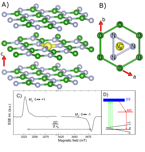
Presently, there is an ongoing exploration of quantum technology systems capable of functioning without sophisticated and expansive cryogenic facilities (at temperatures T 4.2 K) while accommodating a scalable number of qubits. The most recognized spin qubits include the nitrogen-vacancy (NV-) center in diamond [1] and various spin centers found in silicon carbide (SiC) [2]. However, the potential for utilizing electron qubits in conjunction with nuclear spin systems is constrained to a single nitrogen nucleus unless costly isotopic enrichment with nuclei possessing a magnetic moment is employed. In contrast, hexagonal boron nitride (hBN) features nuclei (14N, 11B, 10B) that are each associated with an electron center at a boron vacancy (V), all of which possess a magnetic moment (See Figures 1 A, B). This characteristic may significantly enhance the application of standard CNOT-type operations by leveraging different types of nuclei, thereby facilitating the integration of hBN into quantum computing frameworks [3]. Furthermore, hBN is classified as a two-dimensional (2D) material [4], which enables the utilization of paramagnetic centers situated near the surface, particularly through the combination of microwave and optical radiation, presenting opportunities for advanced ultrasensitive nanosensors [5]. In contrast, in three-dimensional (3D) materials, the proximity of spin centers to the surface tends to degrade their spin coherence time [6]. Additionally, the integration of hBN with other 2D materials has the potential to markedly enhance the sensitivity of these systems to various external influences.
In previous publications from our research group, we demonstrated the efficacy of high-field electron-nuclear double resonance (ENDOR) for both qualitative and quantitative analyses of electron-nuclear interactions in (nano)diamonds [7] and SiC [8]. Our investigation into ENDOR has now been broadened to include hexagonal boron nitride (hBN). Through this extension, we have identified several novel features that had not been observed in earlier studies. This paper aims to elucidate these findings and provide potential explanations for the observed phenomena.
2 Materials
The hBN single crystals with dimensions of 900 m540 m55 m used in this study were commercially produced by the HQ Graphene company. The samples were irradiated at room temperature with 2 MeV electrons to a total dose 6 cm2. No annealing treatments were applied to the irradiated samples.
3 Methods
The electron spin resonance (ESR) experiments were carried out on the W-band (operating at the microwave (MW) frequency of 94 GHz) Bruker Elexsys E680 commercial spectrometer (Karlsruhe, Germany) can be deleted. The ESR spectra in a pulsed mode were registered by detecting the amplitude of the primary electron spin echo (ESE) as a function of the magnetic field sweep using a pulse sequence ––––ESE, where ns and ns. ENDOR spectra were obtained utilizing the Mims pulse sequence
––––––––ESE with a 150 W radiofrequency (RF) generator, where s. Low temperature (=50 K) measurements were conducted by using a flow helium cryostat from Oxford Instruments. The sample’s photoexcitation was provided by green laser ( nm) with an output power of 200 mW.
4 Results and Discussion
ESR spectrum of the V defects in hBN sample under continuous optical excitation and orientation of parallel to the hexagonal axis is presented in Figure 1 C along with the scheme of the spin initialization with the light (Figure 1 D, where ES stands for the excited state, MS is for the metastable state, see reference [4]).
For the ESR spectrum can be described by the following spin-Hamiltonian
| (1) |
where the first two terms determine electronic structure of the spin defect with the -factor and the zero-field splitting (ZFS) constant GHz. The next three terms describe the anisotropic hyperfine interaction (with components , , ) of the electron magnetic moment with the 14N nucleus and the last term is nuclear quadrupole interaction (NQI) , where is the index of the nitrogen nucleus from the three nearest atoms of the immediate environment (Figure 1) [9]. In previous papers [10] the value has been used. The electron and nuclear spins are equal 1. The interaction between the nuclei is neglected.
The experimental ESR spectrum shown in Figure 1 C demonstrates a pair of ESR transitions that serve as fingerprints of the ZFS structure associated with the = 1 for the V defect, manifesting itself by the splitting in magnetic field by the value 2 , where = 3.55 GHz is the zero field splitting of the V defect, and =28 GHz/T is its gyromagnetic ratio. An important feature of the spectrum is that the fine structure components are inverted in phase relative to each other, mimicking a significant deviation of triplet spin sublevels population from Boltzmann statistics due to optical excitation and indicating population inversion, as shown in the scheme presented in Figure 1 D. For the purpose of calculating ENDOR spectra, we take into account only one of the three identical 14N nuclear spins In this alignment of the magnetic field relative to the –axis, the hyperfine coupling has previously been established to be MHz [1, 11]. The last two terms in equation 3 refer to the interaction of the 14N nuclear magnetic moment with the static external magnetic field and the interaction of 14N nuclear electric quadrupole moment with the electric field gradient produced by the surrounding atoms. The nuclear quadrupole constant, which characterizes the the corresponding splitting through nuclear quadrupole interaction (NQI) has been determined to be MHz [11]. To account for the bond direction [10], in the Hamiltonian in crystals coordinates, must be replaced by and by , excluding Zeeman interaction. All three nitrogen nuclei are equivalent for axis, and the summation over these nuclei can be removed. Also, we take into account the closeness of values of and [11, 10], and to facilitate the calculations, we replace by . Creating new variables: , , one can rewrite eq. 1 as
| (2) |
In general, to analyse the ESR spectra, it is sufficient to consider the energy values obtained while neglecting the off-diagonal elements in the spin-Hamiltonian matrix, and these values are presented in equation 3. The corresponding energy level diagram is also shown in Figure 2 with ENDOR transitions indicated by arrows.
| (3) |
Thus, the following transitions should be observed in the ENDOR spectrum:

| (4) |
where the lower index corresponds to ENDOR transition on Figure 2. According to equation 4, one can identify two groups of symmetrical lines (pairs) that have to appear in the ENDOR spectrum. The first set, comprising lines and , is found in proximity to the nuclear Zeeman value (), and the second quadrupole pair ( or ) is positioned near the values. The separation between the pairs within each group is equivalent to 3.
The ENDOR spectra were acquired on both fine structure components low field (): ( mT, lower spectrum) and high field (): ( mT, upper spectrum) as shown in Figure 3 A, B for and ( mT, Figure 3 C, D) for axis. For , the three nitrogen nuclei become nonequivalent (see Figure 1 B), and, therefore, three spectra with slightly different parameters are observed for each type of nuclei. The corresponding lines are designated by upper indices as ’, ”, and ”’. The calculated values for both values and are shown in Figures 3 A,C by green vertical lines. As one can clearly see already from Figure 3, the lines in pairs are arranged asymmetrically relative to the .
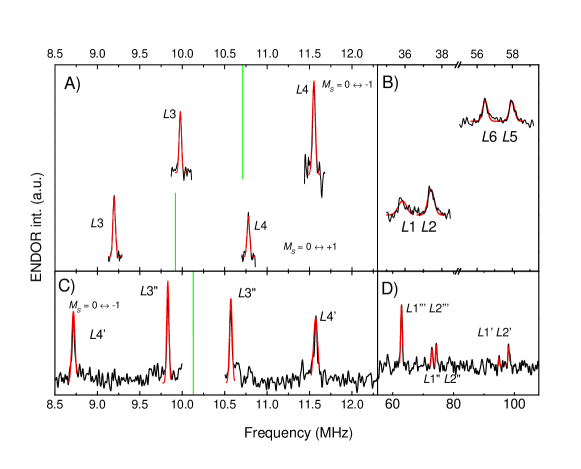
To obtain more accurate numerical parameters of the ENDOR spectra, the observed ENDOR lines are fitted by Gaussian curves (red curves in Figure 3). Positions and widths of the resonant nuclear transitions are summarized in Table 1. Additionally, the pair spliting of lines in pair and the value of center of the pair (pair midpoint) added to Table 1 for comparing with NQI spliting and values of ( mT) = 9.9198 MHz, ( mT) = 10.7120 MHz for and ( mT) = 10.1167 MHz for . The ENDOR linewidth is used to estimate the error bars in the line position designated as .
| N | Frequency, MHz | Spliting of lines in pair, MHz | Midpoint of pair, MHz | |
|---|---|---|---|---|
| mT, | L3 | 9.1980. 005 | 1.580.01 | 9.990.01 |
| L4 | 10.7780. 005 | |||
| L1 | 35.90.2 | 1.60.3 | 36.650.3 | |
| L2 | 37.40.2 | |||
| mT, | L3 | 9.9770. 005 | 1.580.01 | 10.760.01 |
| L4 | 11.5520. 005 | |||
| L5 | 56.50.1 | 1.50.2 | 57.250.2 | |
| L6 | 58.00.1 | |||
| mT, | L3’ | 8.7180. 005 | 2.850.01 | 10.1440.01 |
| L4’ | 11.5710. 005 | |||
| L3” | 9.830. 005 | 0.74280.01 | 10.2010.01 | |
| L4” | 10.57280. 005 |
The data presented in Table 1 indicates that the midpoint of each pair of lines and is displaced towards higher frequencies relative to the Larmor frequency, specifically by approximately MHz for and and MHz respectively, for .
Additionally, the corresponding NQI splitting can be determined as MHz (Table 1) or MHz, with the value calculated as MHz for crystall orientation . For , the value ranges from 2.58 MHz to 0 consistent with the function , where 6o, 54o, and 66o represents the angle between main axis for each nonequivalent type of nitrogen nucleus and magnetic field direction. Note that this study does not consider the non-axiality of the NQI =0.07, resulting in increased by factor time compared to reference [10].
In the following analysis, we will explore the effects of the off-diagonal terms of the spin Hamiltonian matrix by applying perturbation theory. The diagonal segment of the spin Hamiltonian matrix, as outlined in equation 3, will be employed as the initial approximation. As a perturbation operator, we take the lagging off-diagonal part of the spin Hamiltonian matrix:
| (5) |
where , . The wave functions enumerated as
, , , , …, .
In the first order of perturbation theory for the operator , the corrections to the energy values are equal to zero but the wave functions change as
| (6) |
where only the largest variables are left in the denominators. As seen, it results in the mixing the wave functions inside the nuclear triplet with good efficiency 7%, 0.9%, and the hyperfine interaction mixes the electron levels with less efficiency 0.04% or 0.07%.
The energy levels in the second order of perturbation theory can be calculated as
| (7) |
| (8) |
where only the largest terms are left in the denominators. Then the positions (RF frequencies) of the ENDOR lines can be expressed as
| (9) |
The theoretical and experimental data merit a comparative analysis. The ENDOR spectra facilitate the numerical determination of parameters such as = -0.04 MHz, = 0.004 MHz, and = 0.03 MHz. Consequently, for , the calculated line shift is = 0.07 MHz, which aligns closely with the experimentally derived value of MHz. For , the model forecasts a range of line shifts between - = 0.035 MHz to = 0.08 MHz. These values are consistent with the experimental data, which spans from and MHz.
5 Summary
In this investigation, we thoroughly explored the effects of the hyperfine interaction between the electron spin and the three nearest nitrogen atoms (14N) on the resulting ENDOR spectra of the boron vacancy defect V in hBN crystal in the W-band. Measurements of the ENDOR spectra for two crystal orientations reveals that this interaction induces a minor but measurable in the W-band shift in the effective nuclear g-factor of 14N, deviating from its established tabulated value. This shift is accompanied by a corresponding change in the 14N Larmor frequency, which we interpret using second-order perturbation theory. Considering the impact of one type of nuclear sublattice on another is essential when developing algorithms for quantum manipulations that involve electronic and nuclear subsystems. This consideration is particularly relevant in the context of enhancing the precision of temperature and magnetic field measurements, such as those conducted by (nano)sensors utilizing boron defects in hBN.
Acknowledgements.
Financial support of the Russian Science Foundation under Grant RSF 24-12-00151 is acknowledged.References
- [1] Gottscholl A., Kianinia M., Soltamov V., Orlinskii S., Mamin G., Bradac C., Kasper C., Krambrock K., Sperlich A., Toth M., Aharonovich I., Dyakonov V., Nature Materials 19, 540 (2020).
- [2] Astakhov G., Simin D., Dyakonov V., Yavkin B., Orlinskii S., Proskuryakov I., Anisimov A., Soltamov V., Baranov P., Applied Magnetic Resonance 47, 793 (2016).
- [3] Cobarrubia A., Schottle N., Suliman D., Gomez-Barron S., Patino C. R., Kiefer B., Behura S. K., ACS nano 18, 22609 (2024).
- [4] Liu W., Guo N.-J., Yu S., Meng Y., Li Z.-P., Yang Y.-Z., Wang Z.-A., Zeng X.-D., Xie L.-K., Li Q., Wang J.-F., Xu J.-S., Wang Yi-Tao J.-S., Tang, Li C.-F., Guo G.-C. G., Materials for Quantum Technology 2, 032002 (2022).
- [5] Zhang G., Cheng Y., Chou J.-P., Gali A., Applied Physics Reviews 7 (2020).
- [6] Zhang W., Zhang J., Wang J., Feng F., Lin S., Lou L., Zhu W., Wang G., Physical Review B 96, 235443 (2017).
- [7] Yavkin B., Gafurov M., Volodin M., Mamin G., Orlinskii S. B., Experimental Methods in the Physical Sciences 50, 83 (2019).
- [8] Murzakhanov F., Latypova L., Mamin G., Sadovnikova M., von Bardeleben H., Gafurov M., Magnetic Resonance in Solids 26, 24208 (2024).
- [9] MacKenzie K. J., Smith M. E., Multinuclear solid-state nuclear magnetic resonance of inorganic materials, Vol. 6 (Elsevier, 2002) p. 23–108.
- [10] Gracheva I. N., Murzakhanov F. F., Mamin G. V., Sadovnikova M. A., Gabbasov B. F., Mokhov E. N., Gafurov M. R., Journal of Physical Chemistry C 127, 3634 (2023).
- [11] Murzakhanov F. F., Mamin G. V., Orlinskii S. B., Gerstmann U., Schmidt W. G., Biktagirov T., Aharonovich I., Gottscholl A., Sperlich A., Dyakonov V., Soltamov V. A., Nano Letters 22, 2718 (2022).