Long-Lived Coherence between Incoherent Excitons revealed by Time-Resolved ARPES: An Exact Solution

Abstract

We investigate the exciton dynamics in an exactly solvable two-band model for semiconductors. The model incorporates light-matter, electron-electron and electron-phonon interactions, and captures exciton formation as well as the transition from the coherent to the incoherent regime. We analyze excitonic polarization, populations and coherences, with special focus on their impact in Time-Resolved and Angle-Resolved Photoemission Spectroscopy (TR-ARPES). For nonresonant pumping with below-gap photon energies, TR-ARPES spectra reveal distinct excitonic replica and quantum beats persisting in the incoherent regime. These are due to a coherence between different species of incoherent excitons. Such type of coherence is resistant to phonon dephasing, indicating that it follows different dynamics than those governing the coherences considered so far.

I Introduction

Experiments and theoretical advancements in Time-Resolved and Angle-Resolved Photoemission Spectroscopy (TR-ARPES) constitute a highly active field in condensed matter physics [1]. This technique can probe electrons in occupied as well as unoccupied excited states. TR-ARPES has emerged as a powerful experimental tool in diverse areas, including the study of topological insulators [2], carrier dynamics [3], band structure control [4], transient charge-density-wave (CDW) gap melting [5], optical control of spin and valley polarization in excited carriers [6], and exciton dynamics [7, 8, 9]. It has also garnered significant interest from theorists aiming to provide accurate descriptions based on many-body theory [10, 11].

Low-dimensional materials exhibiting excitonic effects demonstrate significant potential for optoelectronic device applications, including electrically driven light emitters, photovoltaic solar cells, photodetectors, and opto-valleytronic devices [12]. Under quasi-resonant excitations, these systems generate a time-dependent polarization [13, 14, 15] which can persist for a few hundreds of femtoseconds [16, 17, 18]. Phonon-assisted polarization-to-population transfer occurs on a sub-picosecond timescale, and it is the key mechanism governing the transition from the coherent to the incoherent regime [13, 14, 19, 15, 20, 21, 22, 23, 24]. During this phase coherent bright excitons are converted into incoherent bright and dark excitons [25, 7]. In the incoherent regime, exciton-phonon [26, 19, 27, 28, 29, 30, 31] and (at high excitation density) exciton-exciton [32, 33, 34, 35] interactions drive the diffusion and, subsequently, the relaxation towards a thermal state [29, 36, 24].

In semiconductors with Rydberg-like excitonic series, two main types of coherences can be distinguished. Ultrafast photoexcitations with below-gap photon-energies cause a transition from the ground state (G) $|\Phi_{g}\rangle$ of energy $E_{g}$ to the quantum superposition state $|\Psi\rangle=\alpha|\Phi_{g}\rangle+\sum_{\lambda}\beta_{\lambda}|X_{\lambda}\rangle$, where $|X_{\lambda}\rangle$ are bright exciton (X) states (one particle-hole over the ground-state) of energy $E_{\lambda}$. At clamped nuclei, the quantum average of an electronic observable $O(t)=\langle\Psi(t)|\hat{O}|\Psi(t)\rangle$ generally oscillates in time with frequencies $(E_{\lambda}-E_{g})$ and $(E_{\lambda}-E_{\lambda^{\prime}})$. The coherent regime refers to the quantum state of matter featuring G-X coherence, leaving unspecified the X-X coherence. Of course, electron-phonon scattering is responsible for suppressing both types of coherence. However, what about the associated time scales? When coherent excitons, $|X\rangle$, are converted into incoherent excitons, $|X^{\rm inc}\rangle$, the G-X coherence vanishes rather than transforming into a G-X^inc coherence. However, could the X-X coherence [37, 38] instead transform into a X^inc-X^inc coherence that persists over longer time scales? If so, the mere absence of coherent excitons would not necessarily indicate the onset a quasi-stationary state.

TR-ARPES offers an invaluable tool to investigate these two different time scales, and to elucidate the nature of what is broadly defined as an “exciton”. In fact, excitonic structures within the gap can exhibit changes in shape, position, and intensity, indicating transitions between excited states with distinct excitonic features. While the incoherent regime has been investigated both theoretically [11, 39, 40, 41] and experimentally [42, 43, 7, 44, 8, 45, 46, 9], the coherent regime has thus far been primarily explored through theoretical frameworks [47, 37, 48, 49, 50, 51] (coherence times in the range of a few hundreds of femtoseconds or shorter make experiments challenging). As for the coherent-to-incoherent crossover, the focus of this work, TR-ARPES remains a ”hic sunt leones” territory.

The coherent-to-incoherent crossover is typically addressed using the excitonic Bloch equations, which is a set of coupled equations for the populations of coherent and incoherent excitons [13, 14, 19, 15, 20, 21, 22, 24]. However, populations alone are not sufficient to extract TR-ARPES spectra. Moreover, these equations neglect X-X coherences from the outset.

In this work we resort to the exact solution of a two-band model with electron-electron and electron-phonon interactions to correlate G-X and X-X coherences with TR-ARPES signatures. Our analysis suggests that phonons suppress the G-X coherence but transform the X-X coherence into a robust X^inc-X^inc coherence, which survives on much longer timescales. Although the two-band model ignores the atomistic details of real excitonic materials, our results indicate that the X^inc-X^inc coherence is significantly more resilient than the G-X one. This effect points to the potential of creating exciton-driven Floquet matter as an alternative approach to Floquet physics in material science.

The plan of the paper is as follows. We discuss the model Hamiltonian in Section II. In Section III we derive the exact time-dependent many-body state along with other quantities like the one-particle Green’s function, the exciton Green’s function and the many-body reduced density matrix. The time evolution of the system is investigated numerically in Section IV for resonant and nonresonant photoexcitations. Finally, we draw our conclusions in Section V.

II Model Hamiltonian

We consider the two-band model Hamiltonian introduced in Ref. [52]:

$$\hat{H}=\hat{H}_{\text{e}}+\hat{H}_{\text{ph}}+\hat{H}_{\text{e-ph}}.$$ (1)

The first term is the pure electronic Hamiltonian,

$$\hat{H}_{\text{e}}=\sum_{\mathbf{k}}(\epsilon^{c}\hat{c}_{\mathbf{k}}^{\dagger}\hat{c}_{\mathbf{k}}+\epsilon_{\mathbf{k}}^{v}\hat{v}_{\mathbf{k}}^{\dagger}\hat{v}_{\mathbf{k}})-\frac{1}{\mathcal{N}}\sum_{{\mathbf{k}}{\mathbf{k}}_{1}{\mathbf{k}}_{2}}\!U_{\mathbf{k}}\;\hat{c}_{{\mathbf{k}}_{1}+{\mathbf{k}}}^{\dagger}\hat{v}_{{\mathbf{k}}_{2}+{\mathbf{k}}}\hat{v}_{{\mathbf{k}}_{2}}^{\dagger}\hat{c}_{{\mathbf{k}}_{1}},$$ (2)

characterized by a flat conduction band and a dispersive valence band, $U_{\mathbf{k}}$ is the Coulomb interaction between conduction-band electrons and valence-band holes, and $\mathcal{N}$ denotes the number of discrete crystal momenta in the first Brillouin zone. The second term is the Hamiltonian of a single phonon mode

$$\hat{H}_{\text{ph}}=\sum_{\mathbf{q}}\omega_{\mathbf{q}}\hat{b}_{\mathbf{q}}^{\dagger}\hat{b}_{\mathbf{q}},$$ (3)

while

$$\hat{H}_{\text{e-ph}}=\frac{1}{\sqrt{\mathcal{N}}}\sum_{{\mathbf{k}}{\mathbf{q}}}(g_{\mathbf{q}}\hat{c}_{{\mathbf{k}}+{\mathbf{q}}}^{\dagger}\hat{c}_{\mathbf{k}}\hat{b}_{\mathbf{q}}+\text{H.c.})$$ (4)

describes the electron-phonon interaction, characterized by a ${\mathbf{k}}$-independent coupling. The flatness of the conduction band and the absence of electron-phonon interactions for electrons in the valence band enable an analytic solution for the time-dependent many-body state, as discussed below. Despite these simplifications, the model correctly captures the formation of coherent excitons, the phonon-induced suppression of G-X coherences and the formation of incoherent excitons [52].

To describe Rydberg-like excitonic series [53, 54] a Yukawa-screened Coulomb interaction is used, $U_{\mathbf{k}}=4\pi u/(|{\mathbf{k}}|^{2}+\kappa^{2})$, where $u$ is the coupling strength and $\kappa$ is the inverse of the screening length. For relatively weak Coulomb interaction compared to the band gap, the ground state $|\Phi_{g}\rangle$ consists of a completely filled valence band and an empty conduction band; we set its energy $E_{g}=0$. In the subspace of one particle-hole states with total momentum ${\mathbf{Q}}$, the electronic Hamiltonian can be diagonalized. The eigenvalue problem is the well known Bethe-Salpeter equation

$$(\epsilon^{c}-\epsilon^{v}_{{\mathbf{k}}})A^{\lambda{\mathbf{Q}}}_{{\mathbf{k}}}-\frac{1}{\mbox{$\mathcal{N}$}}\sum_{{\mathbf{k}}^{\prime}}U_{{\mathbf{k}}-{\mathbf{k}}^{\prime}}A^{\lambda{\mathbf{Q}}}_{{\mathbf{k}}^{\prime}}=E_{\lambda{\mathbf{Q}}}A^{\lambda{\mathbf{Q}}}_{{\mathbf{k}}},$$ (5)

yielding bound excitonic states and unbound electron-hole pair states. In the following, we refer to all types of eigenstates as excitons. They can be written as

$$|X_{\lambda{\mathbf{Q}}}\rangle=\hat{X}^{\dagger}_{\lambda{\mathbf{Q}}}|\Phi_{g}\rangle=\sum_{\mathbf{k}}A^{\lambda{\mathbf{Q}}}_{{\mathbf{k}}}\hat{c}^{\dagger}_{{\mathbf{k}}+{\mathbf{Q}}}\hat{v}_{\mathbf{k}}|\Phi_{g}\rangle.$$ (6)

Due to the flatness of the conduction band, both the wavefunctions and energies are independent of ${\mathbf{Q}}$:

$$A^{\lambda{\mathbf{Q}}}_{{\mathbf{k}}} =A^{\lambda}_{{\mathbf{k}}},$$ (7)

$$E_{\lambda{\mathbf{Q}}} =E_{\lambda}.$$ (8)

The exciton dynamics is initiated by an external pump field. The light-matter coupling is described as:

$$\hat{H}_{\text{light-matter}}(t)=\sum_{{\mathbf{k}}}e(t)d_{\mathbf{k}}\hat{c}_{{\mathbf{k}}}^{\dagger}\hat{v}_{\mathbf{k}}+\text{H.c.},$$ (9)

where $d_{\mathbf{k}}$ is the dipole moment and the electric field of the pump

$$e(t)=e_{0}\sin^{2}\left(\frac{\pi(t-T_{P})}{T_{P}}\right)\sin[\omega_{P}(t-T_{P})]$$ (10)

is active from $t=-T_{P}$ to $t=0$. The pump frequency $\omega_{P}$ will be tuned either to resonate with an exciton or set off-resonance, but still below the gap. In this work, radiative recombination is neglected, hence the total charge in each band is a conserved quantity for positive times.

For simplicity, we assume that electron-phonon scattering is negligible during the pump. This assumption is justified provided that the time-scale for phonon generation is longer than $T_{P}$ (or equivalently, the dynamics during the pump is weakly affected by phonons). Then, for $-T_{P}<t<0$, only bright excitons are generated, and for weak pumps (linear regime) the many-body state of the system reads

$$|\Psi(t)\rangle= \alpha(t)|\Phi_{g}\rangle+\sum_{\lambda}\beta_{\lambda}(t)|X_{\lambda\mathbf{0}}\rangle.$$ (11)

The time-dependent coefficients $\alpha(t)$ and $\beta_{\lambda}(t)$ can easily be obtained numerically by solving the system of linear differential equations:

$$i\dot{\alpha}(t) =\sum_{\lambda}\beta_{\lambda}(t)\Omega^{\ast}_{\lambda}(t),$$ (12)

$$i\dot{\beta}_{\lambda}(t) =E_{\lambda}\beta_{\lambda}(t)+\alpha(t)\Omega_{\lambda}(t),$$

where

$$\Omega_{\lambda}(t)=\sum_{\mathbf{k}}e(t)d_{\mathbf{k}}A_{\mathbf{k}}^{\lambda\ast}.$$ (13)

III Exact Solution

The analytic expression of the time-dependent many-body state of the system for positive times is the first main result of this work. In Appendix A we show that

$$|\Psi(t>0)\rangle =\alpha(0)|\Phi_{g}\rangle+\sum_{\lambda}\beta_{\lambda}(0)\ell(t)e^{-iE_{\lambda}t}$$

$$\times\left(|X_{\lambda\mathbf{0}}\rangle+\sum_{{\mathbf{Q}}}\sqrt{S_{{\mathbf{Q}}}(t)}|X_{\lambda{\mathbf{Q}}}^{\text{inc}}(t)\rangle\right).$$ (14)

Let us examine the physical implications of this result. In Eq. (14), the many-body states $|X_{\lambda{\mathbf{Q}}}^{\text{inc}}(t)\rangle$ of the incoherent $\lambda{\mathbf{Q}}$-excitons, which have so far been characterized solely in terms of populations $N^{\rm inc}_{\lambda{\mathbf{Q}}}$, appear. The explicit form of the states is

$$|X_{\lambda{\mathbf{Q}}}^{\text{inc}}(t)\rangle= \frac{1}{\sqrt{S_{\mathbf{Q}}(t)}}\sum_{M=1}^{\infty}\frac{1}{M!}\sum_{{\mathbf{q}}_{1}\ldots{\mathbf{q}}_{M}}\delta_{{\mathbf{q}}_{1}\ldots+{\mathbf{q}}_{M},-{\mathbf{Q}}}$$

$$\times f_{{\mathbf{q}}_{1}}(t)\ldots f_{{\mathbf{q}}_{M}}(t)\hat{b}^{{\dagger}}_{{\mathbf{q}}_{1}}\ldots\hat{b}^{{\dagger}}_{{\mathbf{q}}_{M}}|X_{\lambda{\mathbf{Q}}}\rangle,$$ (15)

where

$$f_{\mathbf{q}}(t)=\frac{1}{\sqrt{\mathcal{N}}}\frac{g_{\mathbf{q}}}{\omega_{\mathbf{q}}}\left(e^{-i\omega_{\mathbf{q}}t}-1\right)$$ (16)

is the Langreth function [55], and the scattering function

$$S_{\mathbf{Q}}(t)=\frac{1}{\mathcal{N}}\sum_{\mathbf{n}}e^{i{\mathbf{Q}}\cdot{\mathbf{n}}}\exp{\left[\sum_{\mathbf{q}}|f_{\mathbf{q}}(t)|^{2}e^{-i{\mathbf{q}}\cdot{\mathbf{n}}}\right]}-\delta_{{\mathbf{Q}},\mathbf{0}},$$ (17)

is defined in terms of a sum over all unit cell vectors ${\mathbf{n}}$ of the crystal. In Appendix A we show that $S_{\mathbf{Q}}(t)$ is real and strictly positive for all times. According to Eq. (15), the incoherent exciton state is an exciton dressed by a cloud of phonons, more simply referred to as an exciton-polaron. Notice that the total momentum of $|X_{\lambda{\mathbf{Q}}}^{\text{inc}}(t)\rangle$ is zero; the label ${\mathbf{Q}}$ refers to the momentum of the pure electronic part $|X_{\lambda{\mathbf{Q}}}\rangle$, see Eq. (6).

The (bright) coherent, $|X_{\lambda\mathbf{0}}\rangle$, and (momentum-dark) incoherent, $|X_{\lambda{\mathbf{Q}}}^{\text{inc}}(t)\rangle$, exciton states are mutually orthonormal, see Appendix A,

$$\langle X_{\lambda\mathbf{0}}|X_{\lambda^{\prime}\mathbf{0}}\rangle =\delta_{\lambda\lambda^{\prime}},$$ (18a)

$$\langle X_{\lambda{\mathbf{Q}}}^{\text{inc}}(t)|X_{\lambda^{\prime}{\mathbf{Q}}^{\prime}}^{\text{inc}}(t)\rangle =\delta_{\lambda\lambda^{\prime}}\delta_{{\mathbf{Q}},{\mathbf{Q}}^{\prime}},$$ (18b)

$$\langle X_{\lambda\mathbf{0}}|X_{\lambda^{\prime}{\mathbf{Q}}^{\prime}}^{\text{inc}}(t)\rangle =0.$$ (18c)

Therefore, the unitary evolution implies that

$$\left|\beta_{\lambda}(0)\ell(t)\right|^{2}\left(1+\sum_{{\mathbf{Q}}}S_{{\mathbf{Q}}}(t)\right)=1-|\alpha(0)|^{2}.$$ (19)

The function

$$\ell(t)=\exp\left[\frac{1}{\mathcal{N}}\sum_{\mathbf{q}}\left(\frac{g_{\mathbf{q}}}{\omega_{\mathbf{q}}}\right)^{2}\left(-1+e^{-i\omega_{\mathbf{q}}t}+i\omega_{\mathbf{q}}t\right)\right],$$ (20)

is a decaying function of time, see Section IV, and provides the time scale of the G-X coherence, see again Eq. (14). The scattering function $S_{\mathbf{Q}}(t)$ compensates the decay of $\ell(t)$ in such a way that the product $\ell(t)\sqrt{S_{\mathbf{Q}}(t)}$ remains finite in the long time limit, see Eq. (19). Thus, Eq. (14) conveys a clear physical message: electron-phonon scattering causes a depopulation of coherent excitons, which is compensated by an increase of incoherent excitons with finite momentum and finite phonon numbers ($M>0$).

III.1 Exciton states and exciton populations

Our definition of incoherent exciton states is fully consistent with the definitions of coherent and incoherent exciton populations. The total number of excitons is typically written as [56, 24]

$$N_{\lambda{\mathbf{Q}}}\left(t\right)= \langle\Psi(t)|\hat{X}_{\lambda{\mathbf{Q}}}^{\dagger}\hat{X}_{\lambda{\mathbf{Q}}}|\Psi(t)\rangle=\delta_{{\mathbf{Q}},\mathbf{0}}|X_{\lambda\mathbf{0}}(t)|^{2}+N^{\text{inc}}_{\lambda{\mathbf{Q}}}\left(t\right),$$ (21)

where

$$X_{\lambda\mathbf{0}}(t)\equiv\langle\Psi(t)|\hat{X}_{\lambda\mathbf{0}}|\Psi(t)\rangle.$$ (22)

The quantity $X_{\lambda\mathbf{0}}(t)$ is referred to as the excitonic polarization, and its square modulus yields the number of coherent $\lambda$-excitons. From Eq. (14) we find

$$X_{\lambda\mathbf{0}}(t) =\alpha^{*}(0)\sum_{\lambda^{\prime}}\beta_{\lambda^{\prime}}(0)\ell(t)e^{-iE_{\lambda^{\prime}}t}\left\langle\Phi_{g}\right|\hat{X}_{\lambda\mathbf{0}}\left|X_{\lambda^{\prime}\mathbf{0}}\right\rangle$$

$$=\alpha^{*}(0)\beta_{\lambda}(0)\ell(t)e^{-iE_{\lambda}t},$$ (23)

according to which the number of coherent $\lambda$-excitons is

$$N^{\rm coh}_{\lambda}(t)=|X_{\lambda\mathbf{0}}(t)|^{2}=|\beta_{\lambda}(0)\ell(t)|^{2}+\mbox{$\mathcal{O}$}(1-|\alpha(0)|^{2}).$$ (24)

(We recall that in the linear response regime $|\alpha(0)|^{2}$ remains close to unity).

Let us now introduce the projection operators onto the space of coherent and incoherent excitons:

$$\hat{P}^{\rm coh}\equiv\sum_{\lambda}|X_{\lambda\mathbf{0}}\rangle\langle X_{\lambda\mathbf{0}}|,$$ (25)

$$\hat{P}^{\rm inc}(t)\equiv\sum_{\lambda{\mathbf{Q}}}|X^{\rm inc}_{\lambda{\mathbf{Q}}}(t)\rangle\langle X^{\rm inc}_{\lambda{\mathbf{Q}}}(t)|.$$ (26)

Taking into account the orthonormality relations in Eq. (18) we have

$$|\Psi(t)=\alpha(0)|\Phi_{g}\rangle+\hat{P}^{\rm coh}|\Psi(t)\rangle+\hat{P}^{\rm inc}(t)|\Psi(t)\rangle.$$ (27)

It is straightforward to verify that the value of $N^{\rm coh}_{\lambda}(t)$ in Eq. (24) is the same as the exciton number operator averaged over the coherent component of the many-body state, that is

$$\langle\Psi(t)|\hat{P}^{\rm coh}\hat{X}_{\lambda{\mathbf{Q}}}^{\dagger}\hat{X}_{\lambda{\mathbf{Q}}}\hat{P}^{\rm coh}|\Psi(t)\rangle=\delta_{{\mathbf{Q}},\mathbf{0}}|\beta_{\lambda}(0)\ell(t)|^{2}.$$ (28)

Additionally, since the electron-phonon interaction preserves the total number of electrons in each band, we can rewrite Eq. (21) as

$$N_{\lambda{\mathbf{Q}}}(t) =\langle\Psi(t)|\hat{P}^{\rm coh}\hat{X}_{\lambda{\mathbf{Q}}}^{\dagger}\hat{X}_{\lambda{\mathbf{Q}}}\hat{P}^{\rm coh}|\Psi(t)\rangle$$

$$+\langle\Psi(t)|\hat{P}^{\rm inc}(t)\hat{X}_{\lambda{\mathbf{Q}}}^{\dagger}\hat{X}_{\lambda{\mathbf{Q}}}\hat{P}^{\rm inc}(t)|\Psi(t)\rangle.$$ (29)

The first term in this equation coincides with the first term of Eq. (21), see Eqs. (28) and (24), and therefore

$$N^{\rm inc}_{\lambda{\mathbf{Q}}}(t) =\langle\Psi(t)|\hat{P}^{\rm inc}(t)\hat{X}_{\lambda{\mathbf{Q}}}^{\dagger}\hat{X}_{\lambda{\mathbf{Q}}}\hat{P}^{\rm inc}(t)|\Psi(t)\rangle$$

$$=|\beta_{\lambda}(0)\ell(t)|^{2}S_{{\mathbf{Q}}}(t).$$ (30)

It is worth noticing that Eqs. (24) and (30) together with Eq. (19) imply that the total number of excitons remain constant after the pump (positive times):

$$\sum_{\lambda}\left(N^{\rm coh}_{\lambda}(t)+\sum_{{\mathbf{Q}}}N^{\rm inc}_{\lambda{\mathbf{Q}}}(t)\right)={\rm const},\quad t>0.$$ (31)

III.2 One-particle Green’s Function

To calculate the TR-ARPES spectrum we need the one-particle lesser Green’s function, which is defined as

$$G_{cc{\mathbf{k}}}(t,t^{\prime})= i\left\langle\Psi(t^{\prime})\right|\hat{c}_{\mathbf{k}}^{\dagger}e^{-i\hat{H}(t^{\prime}-t)}\hat{c}_{\mathbf{k}}|\Psi(t)\rangle.$$ (32)

Writing the many-body state as in Eq. (27) we see that the cross product between coherent and incoherent states vanish, and therefore

$$G_{cc{\mathbf{k}}}(t,t^{\prime})=G_{cc{\mathbf{k}}}^{\text{coh}}(t,t^{\prime})+G_{cc{\mathbf{k}}}^{\text{inc}}(t,t^{\prime}),$$ (33)

where

$$G_{cc{\mathbf{k}}}^{\text{coh}}(t,t^{\prime})= i\langle\Psi(t^{\prime})|\hat{P}^{\rm coh}\hat{c}_{\mathbf{k}}^{\dagger}e^{-i\hat{H}(t^{\prime}-t)}\hat{c}_{\mathbf{k}}\hat{P}^{\rm coh}|\Psi(t)\rangle$$

$$= i\sum_{\lambda\lambda^{\prime}}\beta_{\lambda}(t)\beta^{\ast}_{\lambda^{\prime}}(t^{\prime})\ell(t)\ell^{\ast}(t^{\prime})A_{\mathbf{k}}^{\lambda}A^{\lambda^{\prime}\ast}_{\mathbf{k}}$$

$$\times e^{-i(\epsilon_{\mathbf{k}}^{v}+E_{\lambda})t}e^{i(\epsilon_{\mathbf{k}}^{v}+E_{\lambda^{\prime}})t^{\prime}},$$ (34)

and

$$G_{cc{\mathbf{k}}}^{\text{inc}}(t,t^{\prime})= i\langle\Psi(t^{\prime})|\hat{P}^{\rm inc}(t^{\prime})\hat{c}_{\mathbf{k}}^{\dagger}e^{-i\hat{H}(t^{\prime}-t)}\hat{c}_{\mathbf{k}}\hat{P}^{\rm inc}(t)|\Psi(t)\rangle$$

$$= \sum_{\mathbf{Q}}S_{\mathbf{Q}}(t,t^{\prime})G_{cc{\mathbf{k}}+{\mathbf{Q}}}^{\text{coh}}(t,t^{\prime}).$$ (35)

The function

$$S_{\mathbf{Q}}(t,t^{\prime})=\frac{1}{\mathcal{N}}\sum_{\mathbf{n}}e^{i{\mathbf{Q}}\cdot{\mathbf{n}}}$$

$$\quad\times\exp{\left[\sum_{\mathbf{q}}f^{*}_{\mathbf{q}}(t^{\prime})f_{\mathbf{q}}(t)e^{-i\omega_{\mathbf{q}}(t^{\prime}-t)-i{\mathbf{q}}\cdot{\mathbf{n}}}\right]}-\delta_{{\mathbf{Q}},0},$$ (36)

extends Eq. (17) away from the time diagonal since

$$S_{\mathbf{Q}}(t,t)=S_{\mathbf{Q}}(t).$$ (37)

The derivation of these results can be found in Appendix B.

For completeness we also report the off-diagonal lesser Green’s function

$$G_{cv{\mathbf{k}}}\left(t,t^{\prime}\right) =i\langle\Psi(t^{\prime})|\hat{v}_{\mathbf{k}}^{\dagger}e^{-i\hat{H}\left(t^{\prime}-t\right)}\hat{c}_{\mathbf{k}}|\Psi(t)\rangle$$

$$=i\alpha^{*}(t^{\prime})\sum_{\lambda}\beta_{\lambda}(t)\ell(t)A^{\lambda}_{\mathbf{k}}e^{-iE_{\lambda}t}e^{i\epsilon_{\mathbf{k}}^{v}\left(t^{\prime}-t\right)}.$$ (38)

Notice that the expressions for the Green’s functions in Eqs. (34,35,38) are valid for all $t$ and $t^{\prime}$ provided that we extend the definition of $\alpha(t)$ and $\beta(t)$ to positive times as

$$\alpha(t>0)=\alpha(0),\quad\beta(t>0)=\beta(0),$$ (39)

and the definition of $f_{{\mathbf{q}}}(t)$ and $\ell(t)$ at negative times as

$$f_{{\mathbf{q}}}(t<0)=0,\quad\ell(t<0)=1.$$ (40)

In Section IV we use the Green’s function to calculate the TR-ARPES signal at pump-probe delay $T$ by Fourier transforming $G_{\mathbf{k}}^{cc}(t,t^{\prime})$ with respect to the relative time $\tau$

$$A_{\mathbf{k}}(T,\omega)=-i\int d\tau e^{i\omega\tau}G_{cc{\mathbf{k}}}\left(T+\frac{\tau}{2},T-\frac{\tau}{2}\right).$$ (41)

The temporal evolution of the spectral function from the overlapping regime to the nonoverlapping incoherent regime is the second main result of this work.

We also use the equal-time Green’s function to calculate the momentum-resolved occupations in the conduction band

$$n_{c{\mathbf{k}}}(t)= -iG_{cc{\mathbf{k}}}(t,t)=n_{c{\mathbf{k}}}^{\text{coh}}(t)+n_{c{\mathbf{k}}}^{\text{inc}}(t),$$ (42)

and the total polarization

$$P(t)=-\frac{i}{\mathcal{N}}\sum_{\mathbf{k}}d_{\mathbf{k}}G_{cv{\mathbf{k}}}(t,t)+\text{ H.c. }$$ (43)

III.3 Excitonic Green’s function

From the exact many-body state we can also calculate the excitonic Green’s function, which is defined according to [24]

$$N_{\lambda\lambda^{\prime}{\mathbf{Q}}}(t,t^{\prime})= \left\langle\Psi(t^{\prime})\right|\hat{X}_{\lambda^{\prime}{\mathbf{Q}}}^{\dagger}e^{-i\hat{H}(t^{\prime}-t)}\hat{X}_{\lambda{\mathbf{Q}}}|\Psi(t)\rangle$$

$$= \delta_{{\mathbf{Q}},\mathbf{0}}N^{\text{coh}}_{\lambda\lambda^{\prime}}(t,t^{\prime})+N_{\lambda\lambda^{\prime}{\mathbf{Q}}}^{\text{inc}}(t,t^{\prime}).$$ (44)

In Appendix B we show that

$$N^{\text{coh}}_{\lambda\lambda^{\prime}}(t,t^{\prime}) =\beta_{\lambda}(t)\beta^{\ast}_{\lambda^{\prime}}(t^{\prime})\ell(t)\ell^{\ast}(t^{\prime})e^{-iE_{\lambda}t+iE_{\lambda^{\prime}}t^{\prime}}$$

$$=X_{\lambda\mathbf{0}}(t)X^{\ast}_{\lambda^{\prime}\mathbf{0}}(t),$$ (45)

and

$$N_{\lambda\lambda^{\prime}{\mathbf{Q}}}^{\text{inc}}(t,t^{\prime})=S_{{\mathbf{Q}}}(t,t^{\prime})N^{\text{coh}}_{\lambda\lambda^{\prime}}(t,t^{\prime}).$$ (46)

The equal-time values of these Green’s functions yield the coherent exciton density matrix

$$N^{\text{coh}}_{\lambda\lambda^{\prime}}(t)\equiv N^{\text{coh}}_{\lambda\lambda^{\prime}}(t,t),$$ (47)

and the incoherent exciton density matrix

$$N^{\text{inc}}_{\lambda\lambda^{\prime}{\mathbf{Q}}}(t)\equiv N^{\text{inc}}_{\lambda\lambda^{\prime}{\mathbf{Q}}}(t,t).$$ (48)

The diagonal values ($\lambda=\lambda^{\prime}$) of the density matrices correctly reduce to the coherent and incoherent exciton populations of Eqs. (24) and (30).

III.4 Many-Body Reduced Density Matrix

To characterized the electronic subsystem at a certain time we also calculate the many-body reduced density matrix, obtained by tracing the full many-body density matrix over the phononic degrees of freedom

$$\hat{\rho}_{\mathrm{el}}(t)=\operatorname{Tr}_{\mathrm{ph}}\{|\Psi(t)\rangle\langle\Psi(t)|\}.$$ (49)

In Appendix B we show that

$$\hat{\rho}_{\mathrm{el}}(t) =|\alpha(t)|^{2}|\Phi_{g}\rangle\langle\Phi_{g}|+\sum_{\lambda\lambda^{\prime}}N^{\text{coh}}_{\lambda\lambda^{\prime}}(t)|X_{\lambda^{\prime}\mathbf{0}}\rangle\langle X_{\lambda\mathbf{0}}|$$

$$+\sum_{\lambda}\left(X_{\lambda\mathbf{0}}(t)|X_{\lambda\mathbf{0}}\rangle\langle\Phi_{g}|+X_{\lambda\mathbf{0}}^{\ast}(t)|\Phi_{g}\rangle\langle X_{\lambda\mathbf{0}}|\right)$$

$$+\sum_{\lambda\lambda^{\prime}{\mathbf{Q}}}N_{\lambda\lambda^{\prime}{\mathbf{Q}}}^{\text{inc}}(t)|X_{\lambda^{\prime}{\mathbf{Q}}}\rangle\langle X_{\lambda{\mathbf{Q}}}|$$ (50)

Using Eq. (19) we can easily check that ${\rm Tr}_{\rm el}[\hat{\rho}_{\mathrm{el}}(t)]=1$ for all times, as it should.

Let us discuss Eq. (50). Immediately after pumping the electronic subsystem exhibits G-X and X-X coherences, with $X_{\lambda\mathbf{0}}(t)$ governing the timescale over which this coherent regime persists. The X-X coherence decays twice as fast since $N^{\text{coh}}_{\lambda\lambda^{\prime}}=X_{\lambda\mathbf{0}}X_{\lambda^{\prime}\mathbf{0}}^{\ast}$. As time passes, both coherent exciton populations and X-X coherences are transferred to incoherent excitons. In the incoherent regime, we report a long-lasting X^inc-X^inc coherence. From Eqs. (46) and (23) we have

$$N_{\lambda\lambda^{\prime}{\mathbf{Q}}}^{\text{inc}}(t) =S_{{\mathbf{Q}}}(t)X_{\lambda\mathbf{0}}(t)X_{\lambda^{\prime}\mathbf{0}}^{\ast}(t)$$

$$=\frac{\beta_{\lambda^{\prime}}^{\ast}(0)}{\beta^{\ast}_{\lambda}(0)}N^{\text{inc}}_{\lambda{\mathbf{Q}}}(t)e^{-i(E_{\lambda}-E_{\lambda^{\prime}})t}.$$ (51)

Taking into account that the total number of excitons remains conserved, see Eq. (31), we see that the X^inc-X^inc coherence does not vanish as time increases. While this conclusion depends on the chosen model Hamiltonian, it suggests that the X^inc-X^inc coherence can be far more robust than one might expect.

IV Results

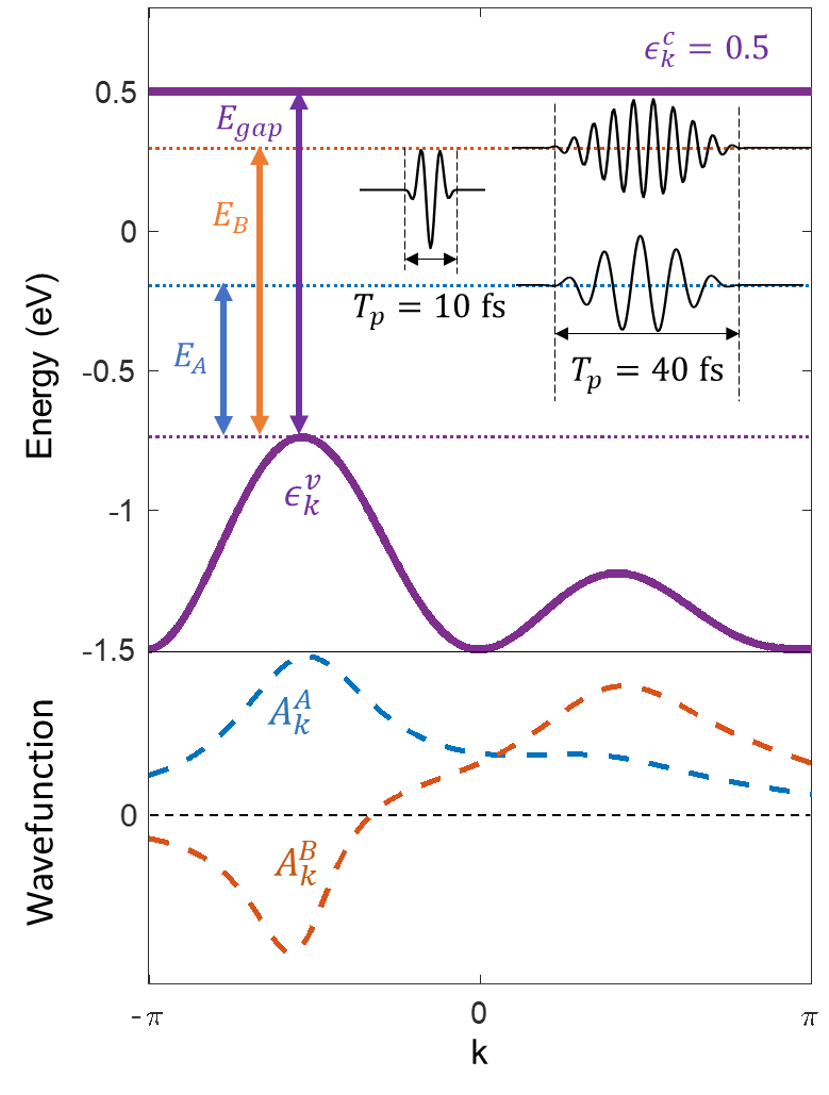
Figure 1: (Top) Band structure and pump profiles. The arrows indicate the energy of the A and B excitons and the gap. For resonant excitations $\omega_{P}=E_{A}=0.54$ eV or $\omega_{P}=E_{B}=1.03$ eV whereas for nonresonant excitations $\omega_{P}=0.99$ eV. (Bottom) Excitonic wavefunctions in momentum space.

We consider a one-dimensional system with a flat conduction band, $\epsilon^{c}_{k}=\epsilon^{c}=0.5$ eV, and a dispersive valence band, $\epsilon_{k}^{v}=\big{(}[1-k/(2\pi)]\cos^{2}{|k+\pi/2|}-1.5\big{)}$ eV, where the dimensionless quasi-momentum $k\in(-\pi,\pi)$. The band structure is illustrated in Fig. 1(top). The valence band has two local maxima, the absolute maximum (VBM) being at energy $-0.74$ eV, and the band gap is $E_{\text{gap}}=1.24$ eV. For the statically screened Coulomb interaction we take $U_{k}=0.3\times{4\pi}/{(k^{2}+1.2^{2})}$ eV, giving rise to two bound exciton states of energy $E_{A}\simeq 0.54$ eV and $E_{B}\simeq 1.03$ eV. The corresponding exciton wavefunctions are shown in Fig. 1(bottom) and resemble the first two eigenstates of a 1D infinite potential well. As for the phonon part, we consider acoustic phonons with dispersion $\omega_{q}=0.45\sin|q|$ eV and an electron-phonon coupling $g_{q}=0.1(\cos q+1)$ eV.

The system is driven out of equilibrium by a pump field with $k$-independent Rabi frequencies $\Omega_{k}=e_{0}d_{k}=10^{-5}$ eV (linear response regime). We study two different pump profiles, as illustrated in Fig. 1(top). All calculations employ $\mathcal{N}=280$ $k$-points to ensure sufficient resolution in momentum space.

IV.1 Resonant Pumping

We tune the pump frequency $\omega_{P}=E_{A}$ in resonance with the A-exciton and set the pump duration $T_{P}\simeq 40$ fs (about five excitonic periods). In Fig. 2(a) we report the population of coherent excitons $|X_{A0}(t)|^{2}$ ($X_{B0}(t)$ is vanishingly small) and the population of incoherent excitons for a few representative $Q$-points. For resonant pumping no X-X coherence exists, and hence no X^inc-X^inc coherence can develop. The excitonic polarization increases monotonically (the superimposed oscillations have the same frequency as the pump pulse) until the end of the pump ($t=0$) and then decreases exponentially due to phonon-induced decoherence: $|X_{A0}(t)|\simeq e^{-t/\tau_{\rm decoh}}$. The decoherence time can be calculated independently [52] and is given by

$$\tau_{\rm decoh}=\frac{2}{g_{0}^{2}}\left.\frac{d\omega_{q}}{dq}\right|_{q=0}\simeq 14.8\;{\rm fs}.$$ (52)

We observe that the excitonic Bloch equations [13, 14, 19, 15, 20, 21, 22, 24] provide a formula for the decoherence time in terms of the so called exciton-phonon coupling. In our two-band model, the exciton-phonon coupling for the scattering $X_{\lambda Q}\to X_{\lambda^{\prime}Q^{\prime}}$ reads

$$\mbox{$\mathcal{G}$}^{\lambda\lambda^{\prime}}(Q,Q^{\prime})=\sum_{k}A^{\lambda Q\ast}_{k}g_{Q^{\prime}-Q}A^{\lambda^{\prime}Q^{\prime}}_{k}=\delta_{\lambda\lambda^{\prime}}g_{Q^{\prime}-Q},$$ (53)

where in the last equality we use that $A^{\lambda Q}_{k}$ is independent of $Q$, see Eq. (7), and that the exciton wavefunctions are orthonormal. This explains the appearance of $g$ instead of $\mathcal{G}$ in Eq. (52). We also emphasize that $1/\tau_{\rm decoh}$ is quadratic in the electron-phonon coupling. Thus, higher order contribution vanish identically for this model Hamiltonian.

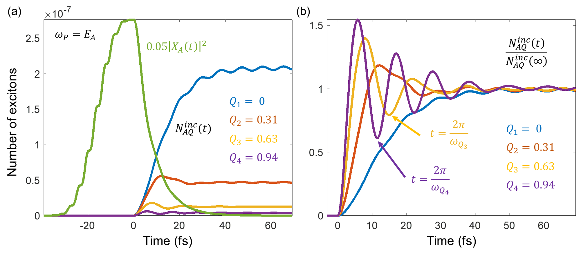
Figure 2: (a) Population of coherent phonons $|X_{A}(t)|^{2}$ and population of incoherent excitons $N^{\text{inc}}_{AQ}(t)$ versus time for resonant excitation at frequency $\omega_{P}=E_{A}=0.54$ eV. (b) Population of incoherent excitons normalized to the asymptotic value.

The decrease of coherent excitons is concomitant with the increase of incoherent (momentum-dark) A-excitons (no B-excitons are generated). The rate of growth depends on the center-of-mass momentum $Q$, and is accompanied by superimposed oscillations of period $2\pi/\omega_{Q}$, see Fig. 2(b). For $t\gtrsim 66$ fs, $X_{A0}(t)$ vanishes, and the system enters the incoherent regime, characterized by the complete absence of G-X coherence. In this regime, only incoherent A-excitons exist. Their populations cease to oscillate and attain a steady value. Interestingly, the steady-state populations are peaked at $Q=0$, despite the fact that the exciton energies are independent of $Q$, see Eq. (8). Although the model investigated is an oversimplification of real excitonic materials, this result highlights that excitonic populations described by a Bose distribution (as predicted by the excitonic Bloch equations) is an approximation. In fact, the extent to which excitons can be approximated as bosons [57, 58], and their potential to condense into a degenerate state, remain open questions.

In Fig. 3(a) we display the momentum-resolved distribution of carriers in the conduction band, see Eq. (42). For negative times $n_{ck}(t)$ grows proportional to the modulus square of the A-exciton wavefunction $|A^{A}_{k}|^{2}$. For $t>0$, the distribution slightly spreads due to phonon dressing.

If the probe pulse duration $T_{p}$ is much longer than typical electronic timescales, and its frequency is sufficiently large to resolve the desired removal energies, the excitonic impact on TR-ARPES in both coherent and incoherent regimes can be numerically calculated from [cfr. Eq. (41)]

$$A_{k}(T,\omega)=-i\int_{T-\frac{\tau_{p}}{2}}^{T+\frac{\tau_{p}}{2}}d\tau e^{i\omega\tau}G_{k}^{cc}\left(T+\frac{\tau}{2},T-\frac{\tau}{2}\right),$$ (54)

where $T$ is the time at which the probe interacts with the system and $\omega$ is the shifted photoemission energy. Henceforth, we refer to $T$ as the pump-probe delay.

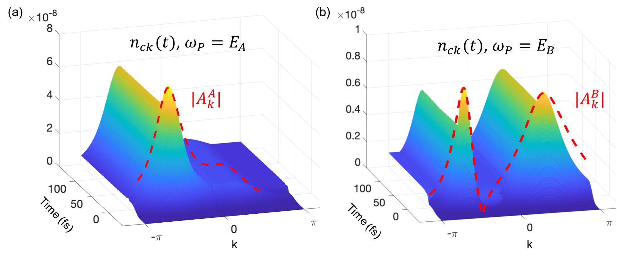
Figure 3: Momentum resolved carrier occupations $n_{k}^{c}(t)$ versus time for resonant excitations with (a) the A exciton [$\omega_{P}=E_{A}=0.54$ eV] and (b) the B exciton [$\omega_{P}=E_{B}=1.03$ eV].

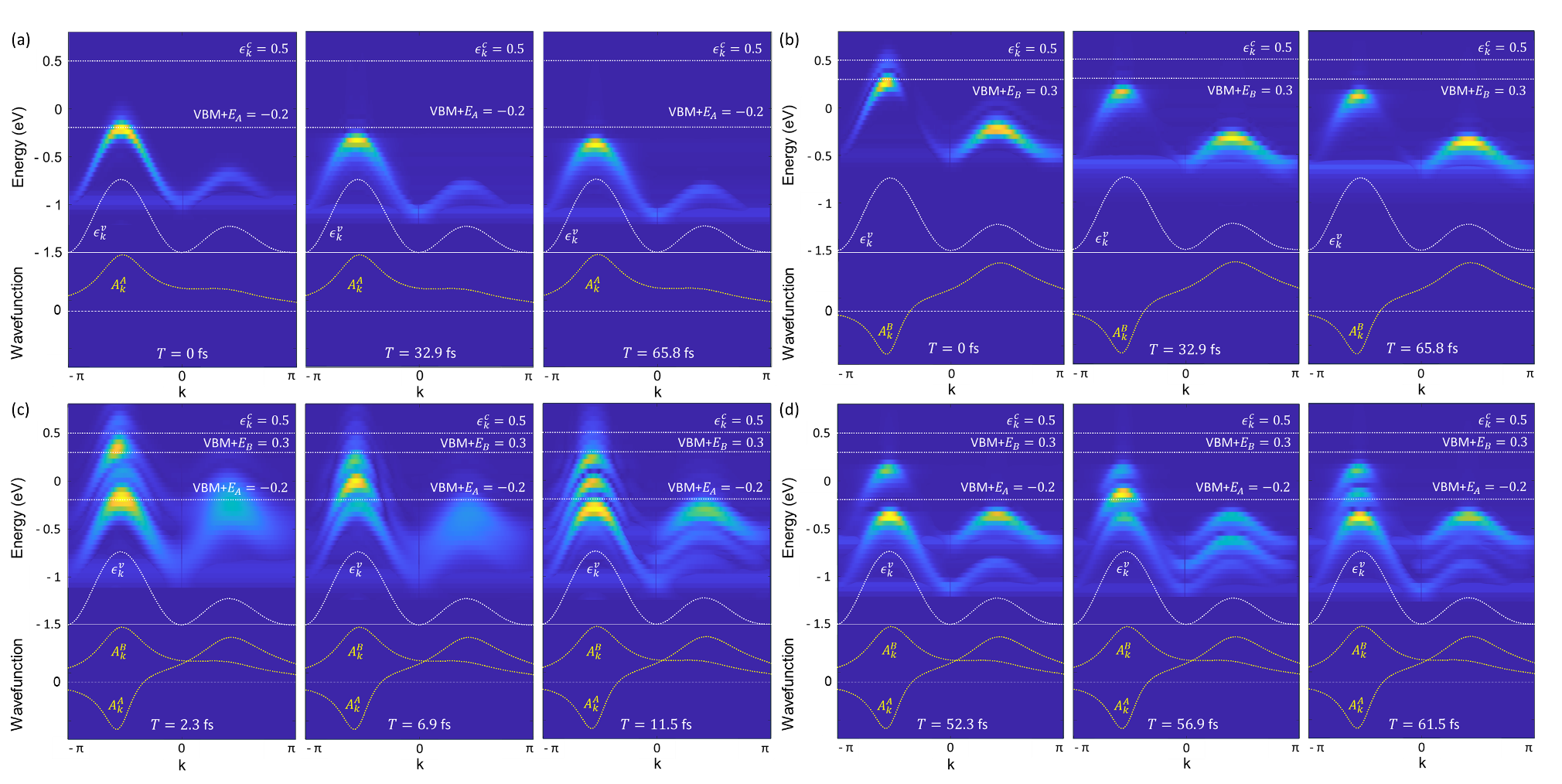
Figure 4: TR-ARPES spectra for different pump-probe delays $T$. The pump is resonant either with the A exciton [$\omega_{P}=E_{A}=0.54$ eV] (a) or the B exciton [$\omega_{P}=E_{B}=1.03$ eV] (b). (c-d) Nonresonant spectra [$\omega_{P}=0.99$ eV]. In each panel the electronic bands (top, dashed lines) and exciton wavefunctions (bottom) are displayed.

We choose the probe duration $T_{p}=80$ fs, significantly longer than the excitonic timescales $2\pi/E_{\lambda}$ for both the A- and B-exciton. The TR-ARPES spectra is shown in Fig. 4(a). The exact solution allows us to follow the temporal evolution of the spectral properties. In particular, in the overlapping regime (zero pump-probe delay) we clearly distinguish the excitonic replica of the valence band shifted upward by the A-exciton energy $E_{A}$ [11]. The spectral weight of the replica is proportional to the modulus square of the excitonic wavefunctions$|A^{A}_{k}|^{2}$, and its position is slightly renormalized by the optical field. As the system enters the incoherent regime ($T\simeq 66$ fs), the excitonic replica exhibits a downward Stokes shift [59] and broadens. This is consistent with the fact that incoherent excitons are excitons dressed by phonons (or exciton-polarons), see Eq. (15).

Pumping in resonance with the B-exciton yields a similar behavior. In fact, phonon-mediated scattering between different exciton species is not allowed in the investigated model. As already observed, the exciton-phonon coupling for the transition $BQ\to AQ^{\prime}$ vanishes, see Eq. (53).

We have performed simulations with pump frequency $\omega_{P}=E_{B}$ and pump duration $T_{P}\simeq 40$ fs. In Fig. 3(b) we display the evolution of the momentum resolved carrier density, highlighting the profile of the modulus square of the B-exciton wavefunction. In Fig. 4(b) we display the evolution of the TR-ARPES spectrum. We observe the excitonic replica at energy $E_{B}$ above the VBM, and the Stokes shift in the incoherent regime. Since $|A^{B}_{k}|^{2}$ has two well pronounced maxima in correspondence of the local valleys of the valence band, the signal intensities from both valleys are comparable.

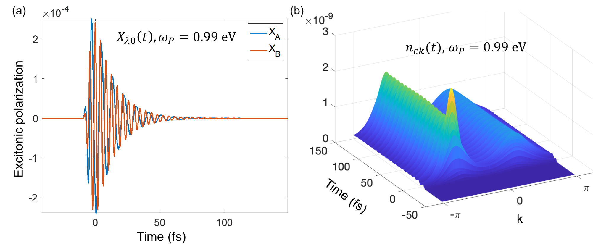
Figure 5: (a) Exciton polarizations and (b) momentum-resolved carrier occupation versus time for nonresonant pumping.

IV.2 Nonresonant pumping

We now address the nonresonant case. We tune the pump frequency between the A- and B-exciton energy, $\omega_{P}=0.99$ eV, and set the pump duration $T_{p}=10$ fs. In Fig. 5(a) we show the excitonic polarizations of the two excitons. The decay rates are identical due to the diagonal exciton-phonon coupling, see Eq. (53), and because the electron-phonon interaction depends solely on the momentum transfer. Interestingly, for the model under investigation, the decay rates predicted by the excitonic Bloch equations are also identical.

The momentum-resolved carrier distribution exhibits oscillations surviving in the incoherent regimes, see Fig. 5(b). Although the G-X and X-X coherences vanish after $\sim 66$ fs, the X-X coherence transforms into a X^inc-X^inc coherence. In the incoherent regime carriers bounce back and forth between the two incoherent exciton states, giving rise to persistent oscillations.

Figure 4(c,d) illustrates the time-resolved spectral function in the overlapping ($T<40$ fs) and nonoverlapping ($T>40$ fs) regimes. As pointed out in Ref. [48], capturing the G-X coherence in TR-ARPES necessitates the use of ultrashort probe pulses. Therefore, we here focus on the X-X coherence. In the absence of electron-phonon coupling, this situation has been analyzed in Ref. [37]: one would observe three excitonic replica, two located at energies $E_{A}$ and $E_{B}$ above the VBM, with intensities proportional to the square modulus of the excitonic wavefunctions, and a third at energy $(E_{A}+E_{B})/2$ above the VBM, with an intensity that oscillates with period $2\pi/(E_{B}-E_{A})$. The quantum beats of the third excitonic replica are the signature of X-X coherence in TR-ARPES. In the presence of electron-phonon coupling our results show that the X-X coherence gradually transforms into a robust X^inc-X^inc coherence, which persists indefinitely, indicating that the system does not attain a steady state. The conversion X-X$\to$X^inc-X^inc is supported by several lines of evidence: (i) no coherent excitons exist for $t>66$ fs, see Fig. 5(a) and (ii) the position of the three excitonic replicas moves downward in energy due to the Stokes shift.

The different outcome of all observable quantities between the resonant and nonresonant pumping scenarios is rooted in the many-body reduced density matrix, see Eq. (50). In the long-time limit the G-X and X-X coherences vanish, and therefore

$$\lim_{t\rightarrow\infty} \hat{\rho}_{\mathrm{el}}(t)=|\alpha(0)|^{2}|\Phi_{g}\rangle\langle\Phi_{g}|+\sum_{\lambda\lambda^{\prime}{\mathbf{Q}}}N_{\lambda\lambda^{\prime}{\mathbf{Q}}}^{\text{inc}}(t)|X_{\lambda^{\prime}{\mathbf{Q}}}\rangle\langle X_{\lambda{\mathbf{Q}}}|.$$ (55)

The long-time limit behavior of the incoherent excitonic density matrix is, see Eq. (51),

$$N_{\lambda\lambda^{\prime}{\mathbf{Q}}}(t\to\infty)=N_{\lambda\lambda^{\prime}{\mathbf{Q}}}^{\infty}e^{-i(E_{\lambda}-E_{\lambda^{\prime}})t},$$ (56)

where the asymptotic (time-independent) matrix $N_{\lambda\lambda^{\prime}{\mathbf{Q}}}^{\infty}$ is history-dependent. Pumping resonantly with the $\lambda_{0}$ exciton we find $N_{\lambda\lambda^{\prime}{\mathbf{Q}}}^{\infty}=\delta_{\lambda\lambda_{0}}\delta_{\lambda^{\prime}\lambda_{0}}N_{\lambda_{0}{\mathbf{Q}}}$, and therefore $\hat{\rho}_{\mathrm{el}}$ in Eq. (55) as well as all observable quantities attain a constant value. In contrast, for nonresonant pumping $N_{\lambda\lambda^{\prime}{\mathbf{Q}}}^{\infty}$ is an off-diagonal matrix. These results suggest that the X^inc-X^inc coherence follows different dynamics than those governing the G-X and X-X coherences.

V Summary and Conclusions

We have considered a two-band semiconductor model Hamiltonian that includes both electron-electron and electron-phonon interactions. Under simplifying assumptions, such as a flat conduction band and the neglect of electron-phonon scattering in the valence band, we have derived several exact results in the weak pumping scenario. Specifically, we present analytic expressions for the many-body state, the one-particle Green’s function, and the exciton Green’s function.

The explicit form of the many-body state provides a rigorous mathematical definition of concepts such as coherent and incoherent excitons. In particular, coherent excitons are quantum superpositions of ground state and pure exciton states, whereas incoherent excitons are exciton states that are dressed by a phonon cloud (exciton-polaron).

Below gap optical excitations generate coherent excitons, and hence G-X and X-X coherence. Phonon-induced dephasing suppresses G-X coherence and converts X-X coherence into a coherence between incoherent excitons. For the investigated model the X^inc-X^inc coherence is resistant to phonon-induced dephasing and persists indefinitely. Quantum beats in the incoherent regime have been reported in carrier populations and TR-ARPES signal.

Although the investigated model is a simplification of the first-principles Hamiltonian of real semiconductors, it correctly captures key universal features, such as the the formation of coherent excitons and their subsequent decay into incoherent (bright and dark) excitons. Our results indicate that the X^inc-X^inc coherence might decay on a timescale significantly longer than that of the excitonic coherences considered to date. The long-lived (several picoseconds) coherence observed in time-resolved optical experiments [60, 61, 62] may be explained in this context. Learning how to control and manipulate excitonic coherence could also enable the exploration of exciton-driven Floquet matter for quantum technology.

Appendix A Analytic Time-Dependent Many-Body State

Starting from the termination of the external pump field, the many-body state evolves like

$$|\Psi(t>0)\rangle= \alpha(0)|\Phi_{g}\rangle+\sum_{\lambda}\beta_{\lambda}(0)e^{-i\hat{H}t}|X_{\lambda\mathbf{0}}\rangle.$$ (57)

We expand the evolved state by a total momentum conserved phonon dressed exciton states

$$e^{-i\hat{H}t}|X_{\lambda\mathbf{0}}\rangle= \sum_{M=0}^{\infty}\frac{1}{M!}\sum_{\lambda{\mathbf{q}}_{1}\ldots{\mathbf{q}}_{M}}\hat{b}^{{\dagger}}_{{\mathbf{q}}_{1}}\ldots\hat{b}^{{\dagger}}_{{\mathbf{q}}_{M}}|X_{\lambda-{\mathbf{q}}_{1}\ldots-{\mathbf{q}}_{M}}\rangle\langle X_{\lambda-{\mathbf{q}}_{1}\ldots-{\mathbf{q}}_{M}}|\hat{b}_{{\mathbf{q}}_{M}}\ldots\hat{b}_{{\mathbf{q}}_{1}}e^{-i\hat{H}t}|X_{\lambda\mathbf{0}}\rangle,$$ (58)

with orthonormality relations

$$\langle X_{\lambda{\mathbf{Q}}}|X_{\lambda^{\prime}{\mathbf{Q}}^{\prime}}\rangle =\langle\Psi_{g}|\hat{X}_{\lambda{\mathbf{Q}}}\hat{X}^{{\dagger}}_{\lambda^{\prime}{\mathbf{Q}}^{\prime}}|\Psi_{g}\rangle$$

$$=\sum_{{\mathbf{k}}{\mathbf{k}}^{\prime}}A^{\lambda*}_{{\mathbf{k}}}A^{\lambda^{\prime}}_{{\mathbf{k}}^{\prime}}\langle\Psi_{g}|\hat{v}^{{\dagger}}_{{\mathbf{k}}}\hat{c}_{{\mathbf{k}}+{\mathbf{Q}}}\hat{c}^{{\dagger}}_{{\mathbf{k}}^{\prime}+{\mathbf{Q}}^{\prime}}\hat{v}_{{\mathbf{k}}^{\prime}}|\Psi_{g}\rangle$$

$$=\delta_{\lambda\lambda^{\prime}}\delta_{{\mathbf{Q}},{\mathbf{Q}}^{\prime}},$$ (59)

and

$$\langle X_{\lambda{\mathbf{Q}}}|\hat{b}_{{\mathbf{q}}_{M}}\ldots\hat{b}_{{\mathbf{q}}_{1}}\hat{b}^{{\dagger}}_{{\mathbf{q}}_{1}^{\prime}}\ldots\hat{b}^{{\dagger}}_{{\mathbf{q}}_{M^{\prime}}^{\prime}}|X_{\lambda^{\prime}{\mathbf{Q}}^{\prime}}\rangle=\delta_{MM^{\prime}}\delta_{\lambda\lambda^{\prime}}\delta_{{\mathbf{Q}},{\mathbf{Q}}^{\prime}}\sum_{P}\prod_{j=1}^{M}\delta_{{\mathbf{q}}_{j},{\mathbf{q}}_{P(j)}^{\prime}}.$$ (60)

From Eq. (58) we can generate a hierarchy of differential equations for the amplitudes

$$\quad i\frac{d}{dt}\langle X_{\lambda-{\mathbf{q}}_{1}\ldots-{\mathbf{q}}_{M}}|\hat{b}_{{\mathbf{q}}_{M}}\ldots\hat{b}_{{\mathbf{q}}_{1}}e^{-i\hat{H}t}|X_{\lambda\mathbf{0}}\rangle$$

$$=\langle X_{\lambda-{\mathbf{q}}_{1}\ldots-{\mathbf{q}}_{M}}|\hat{b}_{{\mathbf{q}}_{M}}\ldots\hat{b}_{{\mathbf{q}}_{1}}\hat{H}e^{-i\hat{H}t}|X_{\lambda\mathbf{0}}\rangle$$

$$=(E_{\lambda}+\sum_{j=1}^{M}\omega_{{\mathbf{q}}_{j}})\langle X_{\lambda-{\mathbf{q}}_{1}\ldots-{\mathbf{q}}_{M}}|\hat{b}_{{\mathbf{q}}_{M}}\ldots\hat{b}_{{\mathbf{q}}_{1}}e^{-i\hat{H}t}|X_{\lambda\mathbf{0}}\rangle$$

$$\quad+\sum_{j=1}^{M}\frac{g_{{\mathbf{q}}_{j}}}{\sqrt{\mbox{$\mathcal{N}$}}}\langle X_{\lambda-{\mathbf{q}}_{1}\ldots-\stackrel{{\scriptstyle\sqcap}}{{{\mathbf{q}}}}_{j}\ldots-{\mathbf{q}}_{M}}|\hat{b}_{{\mathbf{q}}_{M}}\ldots\stackrel{{\scriptstyle\sqcap}}{{\hat{b}}}_{{\mathbf{q}}_{j}}\ldots\hat{b}_{{\mathbf{q}}_{1}}e^{-i\hat{H}t}|X_{\lambda\mathbf{0}}\rangle$$

$$\quad+\sum_{{\mathbf{q}}}\frac{g_{{\mathbf{q}}}}{\sqrt{\mbox{$\mathcal{N}$}}}\langle X_{\lambda-{\mathbf{q}}-{\mathbf{q}}_{1}\ldots-{\mathbf{q}}_{M}}|\hat{b}_{{\mathbf{q}}_{M}}\ldots\hat{b}_{{\mathbf{q}}_{1}}\hat{b}_{{\mathbf{q}}}e^{-i\hat{H}t}|X_{\lambda\mathbf{0}}\rangle.$$ (61)

If we look for solutions of the form

$$\langle X_{\lambda-{\mathbf{q}}_{1}\ldots-{\mathbf{q}}_{M}}|\hat{b}_{{\mathbf{q}}_{M}}\ldots\hat{b}_{{\mathbf{q}}_{1}}e^{-i\hat{H}t}|X_{\lambda\mathbf{0}}\rangle=f_{{\mathbf{q}}_{1}}(t)\ldots f_{{\mathbf{q}}_{M}}(t)\ell(t)e^{-iE_{\lambda}t},$$ (62)

the dynamics of excitons and phonons is decoupled and the hierarchy is solved analytically by solving

$$i\dot{f}_{\mathbf{q}}(t) =\frac{g_{\mathbf{q}}}{\sqrt{\mbox{$\mathcal{N}$}}}+\omega_{\mathbf{q}}f_{\mathbf{q}}(t),$$ (63)

$$i\dot{\ell}(t) =\sum_{\mathbf{q}}\frac{g_{\mathbf{q}}}{\sqrt{\mbox{$\mathcal{N}$}}}f_{\mathbf{q}}(t)\ell(t).$$

The solutions of Eq. (63) with boundary condition $f_{\mathbf{q}}(0)=0$ and $\ell(0)=1$ are

$$f_{\mathbf{q}}(t) =\frac{1}{\sqrt{\mathcal{N}}}\frac{g_{\mathbf{q}}}{\omega_{\mathbf{q}}}\left(e^{-i\omega_{\mathbf{q}}t}-1\right),$$ (64)

$$\ell(t) =\exp\left[\frac{1}{\mathcal{N}}\sum_{\mathbf{q}}\left(\frac{g_{\mathbf{q}}}{\omega_{\mathbf{q}}}\right)^{2}\left(-1+e^{-i\omega_{\mathbf{q}}t}+i\omega_{\mathbf{q}}t\right)\right].$$

Therefore, the analytic expression of the time-dependent many-body state of the system for positive time is

$$|\Psi(t>0)\rangle=\alpha(0)|\Phi_{g}\rangle+\sum_{\lambda}\beta_{\lambda}(0)\ell(t)e^{-iE_{\lambda}t}\sum_{M=0}^{\infty}\frac{1}{M!}\sum_{{\mathbf{q}}_{1}\ldots{\mathbf{q}}_{M}}f_{{\mathbf{q}}_{1}}(t)\ldots f_{{\mathbf{q}}_{M}}(t)\hat{b}^{{\dagger}}_{{\mathbf{q}}_{1}}\ldots\hat{b}^{{\dagger}}_{{\mathbf{q}}_{M}}|X_{\lambda-{\mathbf{q}}_{1}\ldots-{\mathbf{q}}_{M}}\rangle.$$ (65)

We separate out the contribution with zero phonons from the second term

$$|\Psi(t>0)\rangle=\alpha(0)|\Phi_{g}\rangle+\sum_{\lambda}\beta_{\lambda}(0)\ell(t)e^{-iE_{\lambda}t}\left(|X_{\lambda\mathbf{0}}\rangle+\sum_{\mathbf{Q}}|\bar{X}_{\lambda{\mathbf{Q}}}^{\text{inc}}(t)\rangle\right),$$ (66)

where the definition of coherent exciton states $|X_{\lambda\mathbf{0}}\rangle$ is given in Eq. (6), and the unnormalized incoherent exciton states are given by

$$|\bar{X}_{\lambda{\mathbf{Q}}}^{\text{inc}}(t)\rangle=\sum_{M=1}^{\infty}\frac{1}{M!}\sum_{{\mathbf{q}}_{1}\ldots{\mathbf{q}}_{M}}\delta_{{\mathbf{q}}_{1}\ldots+{\mathbf{q}}_{M},-{\mathbf{Q}}}f_{{\mathbf{q}}_{1}}(t)\ldots f_{{\mathbf{q}}_{M}}(t)\hat{b}^{{\dagger}}_{{\mathbf{q}}_{1}}\ldots\hat{b}^{{\dagger}}_{{\mathbf{q}}_{M}}|{X}_{\lambda{\mathbf{Q}}}\rangle.$$ (67)

According to Eq. (60) the coherent and incoherent exciton states are orthogonal

$$\langle X_{\lambda\mathbf{0}}|\bar{X}^{\rm inc}_{\lambda^{\prime}{\mathbf{Q}}^{\prime}}\rangle=0.$$ (68)

Let us normalize the incoherent exciton states. The inner product is

$$\langle\bar{X}_{\lambda{\mathbf{Q}}}^{\text{inc}}(t)|\bar{X}_{\lambda^{\prime}{\mathbf{Q}}^{\prime}}^{\text{inc}}(t)\rangle =\sum_{M,M^{\prime}=1}^{\infty}\frac{1}{M!M^{\prime}!}\sum_{\begin{subarray}{c}{\mathbf{q}}_{1}\ldots{\mathbf{q}}_{M}\\ {\mathbf{q}}_{1}^{\prime}\ldots{\mathbf{q}}_{M^{\prime}}^{\prime}\end{subarray}}\delta_{{\mathbf{q}}_{1}\ldots+{\mathbf{q}}_{M},-{\mathbf{Q}}}\delta_{{\mathbf{q}}_{1}^{\prime}\ldots+{\mathbf{q}}_{M^{\prime}}^{\prime},-{\mathbf{Q}}^{\prime}}f_{{\mathbf{q}}_{1}^{\prime}}(t)\ldots f_{{\mathbf{q}}_{M^{\prime}}^{\prime}}(t)f^{*}_{{\mathbf{q}}_{1}}(t)\ldots f^{*}_{{\mathbf{q}}_{M}}(t)$$

$$\quad\times\langle X_{\lambda{\mathbf{Q}}}|\hat{b}_{{\mathbf{q}}_{M}}\ldots\hat{b}_{{\mathbf{q}}_{1}}\hat{b}^{{\dagger}}_{{\mathbf{q}}_{1}^{\prime}}\ldots\hat{b}^{{\dagger}}_{{\mathbf{q}}_{M^{\prime}}^{\prime}}|X_{\lambda^{\prime}{\mathbf{Q}}^{\prime}}\rangle.$$ (69)

Taking into account Eq. (60), we have

$$\langle\bar{X}_{\lambda{\mathbf{Q}}}^{\text{inc}}(t)|\bar{X}_{\lambda^{\prime}{\mathbf{Q}}^{\prime}}^{\text{inc}}(t)\rangle =\delta_{\lambda\lambda^{\prime}}\delta_{{\mathbf{Q}},{\mathbf{Q}}^{\prime}}\sum_{M=1}^{\infty}\frac{1}{M!}\sum_{{{\mathbf{q}}_{1}\ldots{\mathbf{q}}_{M}}}\delta_{{\mathbf{q}}_{1}\ldots+{\mathbf{q}}_{M},-{\mathbf{Q}}}|f_{{\mathbf{q}}_{1}}(t)|^{2}\ldots|f_{{\mathbf{q}}_{M}}(t)|^{2}.$$ (70)

We rewrite the Kronecker delta function in terms of its discrete Fourier transform

$$\delta_{{\mathbf{q}}_{1}\ldots+{\mathbf{q}}_{M},-{\mathbf{Q}}}=\frac{1}{\mbox{$\mathcal{N}$}}\sum_{{\mathbf{n}}}e^{-i({\mathbf{q}}_{1}\ldots+{\mathbf{q}}_{M}-{\mathbf{Q}})\cdot{\mathbf{n}}},$$ (71)

where ${\mathbf{n}}$ are unit cell vectors. The inner product then takes the compact form

$$\langle\bar{X}_{\lambda{\mathbf{Q}}}^{\text{inc}}(t)|\bar{X}_{\lambda^{\prime}{\mathbf{Q}}^{\prime}}^{\text{inc}}(t)\rangle =\delta_{\lambda\lambda^{\prime}}\delta_{{\mathbf{Q}},{\mathbf{Q}}^{\prime}}\frac{1}{\mbox{$\mathcal{N}$}}\sum_{{\mathbf{n}}}e^{i{\mathbf{Q}}\cdot{\mathbf{n}}}\sum_{M=1}^{\infty}\frac{1}{M!}\left(\sum_{{{\mathbf{q}}}}|f_{{\mathbf{q}}}(t)|^{2}e^{-i{\mathbf{q}}\cdot{\mathbf{n}}}\right)^{M}=\delta_{\lambda\lambda^{\prime}}\delta_{{\mathbf{Q}},{\mathbf{Q}}^{\prime}}S_{\mathbf{Q}}(t),$$ (72)

where

$$S_{\mathbf{Q}}(t)=\frac{1}{\mathcal{N}}\sum_{\mathbf{n}}e^{i{\mathbf{Q}}\cdot{\mathbf{n}}}\exp{\left[\sum_{\mathbf{q}}|f_{\mathbf{q}}(t)|^{2}e^{-i{\mathbf{q}}\cdot{\mathbf{n}}}\right]}-\delta_{{\mathbf{Q}},\mathbf{0}}.$$ (73)

Hence the function $S_{\mathbf{Q}}(t)$ is real and nonnegative for all times. Normalizing the incoherent exciton state as

$$|{X}_{\lambda{\mathbf{Q}}}^{\text{inc}}(t)\rangle=\frac{1}{\sqrt{S_{\mathbf{Q}}(t)}}|\bar{X}_{\lambda{\mathbf{Q}}}^{\text{inc}}(t)\rangle,$$ (74)

we eventually obtain the time-dependent many-body state

$$|\Psi(t>0)\rangle =\alpha(0)|\Phi_{g}\rangle+\sum_{\lambda}\beta_{\lambda}(0)\ell(t)e^{-iE_{\lambda}t}\left(|X_{\lambda\mathbf{0}}\rangle+\sum_{{\mathbf{Q}}}\sqrt{S_{{\mathbf{Q}}}(t)}|X_{\lambda{\mathbf{Q}}}^{\text{inc}}(t)\rangle\right)$$ (75)

with orthonormal relations

$$\langle X_{\lambda\mathbf{0}}|X_{\lambda^{\prime}\mathbf{0}}\rangle =\delta_{\lambda\lambda^{\prime}},$$ (76a)

$$\langle X_{\lambda{\mathbf{Q}}}^{\text{inc}}(t)|X_{\lambda^{\prime}{\mathbf{Q}}^{\prime}}^{\text{inc}}(t)\rangle =\delta_{\lambda\lambda^{\prime}}\delta_{{\mathbf{Q}},{\mathbf{Q}}^{\prime}},$$ (76b)

$$\langle X_{\lambda\mathbf{0}}|X_{\lambda^{\prime}{\mathbf{Q}}^{\prime}}^{\text{inc}}(t)\rangle =0.$$ (76c)

Appendix B Green’s Function

B.1 One-particle Green’s Function

We calculate the one-particle lesser Green’s function defined in Eqs. (32) and (33). For the coherent contribution we have

$$G_{cc{\mathbf{k}}}^{\text{coh}}(t,t^{\prime})= i\langle\Psi(t^{\prime})|\hat{P}^{\rm coh}\hat{c}_{\mathbf{k}}^{\dagger}e^{-i\hat{H}(t^{\prime}-t)}\hat{c}_{\mathbf{k}}\hat{P}^{\rm coh}|\Psi(t)\rangle$$

$$= i\sum_{\lambda\lambda^{\prime}}\beta_{\lambda}(t)\beta_{\lambda^{\prime}}^{*}(t^{\prime})\ell(t)\ell^{*}(t^{\prime})e^{-iE_{\lambda}t}e^{iE_{\lambda^{\prime}}t^{\prime}}\langle X_{\lambda^{\prime}\mathbf{0}}|\hat{c}_{\mathbf{k}}^{\dagger}e^{-i\hat{H}(t^{\prime}-t)}\hat{c}_{\mathbf{k}}|X_{\lambda\mathbf{0}}\rangle.$$ (77)

The state $\hat{c}_{\mathbf{k}}|X_{\lambda\mathbf{0}}\rangle$ is an eigenstate of $\hat{H}$ with a ${\mathbf{k}}$-momentum hole:

$$e^{-i\hat{H}(t^{\prime}-t)}\hat{c}_{\mathbf{k}}|X_{\lambda\mathbf{0}}\rangle =A_{\mathbf{k}}^{\lambda}e^{-i(-\epsilon_{\mathbf{k}}^{v})(t^{\prime}-t)}\hat{v}_{\mathbf{k}}|\Phi_{g}\rangle.$$ (78)

Hence the coherent contribution of the one-particle Green’s function is given by

$$G_{cc{\mathbf{k}}}^{\text{coh}}(t,t^{\prime})= i\sum_{\lambda\lambda^{\prime}}\beta_{\lambda}(t)\beta^{\ast}_{\lambda^{\prime}}(t^{\prime})\ell(t)\ell^{\ast}(t^{\prime})A_{\mathbf{k}}^{\lambda}A^{\lambda^{\prime}\ast}_{\mathbf{k}}e^{-i(\epsilon_{\mathbf{k}}^{v}+E_{\lambda})t}e^{i(\epsilon_{\mathbf{k}}^{v}+E_{\lambda^{\prime}})t^{\prime}}.$$ (79)

For the incoherent contribution we have

$$G_{cc{\mathbf{k}}}^{\rm inc}(t,t^{\prime})= i\langle\Psi(t^{\prime})|\hat{P}^{\rm inc}\hat{c}_{\mathbf{k}}^{\dagger}e^{-i\hat{H}(t^{\prime}-t)}\hat{c}_{\mathbf{k}}\hat{P}^{\rm inc}|\Psi(t)\rangle$$

$$= i\sum_{\lambda\lambda^{\prime}}\beta_{\lambda}(t)\beta_{\lambda^{\prime}}^{*}(t^{\prime})\ell(t)\ell^{*}(t^{\prime})e^{-iE_{\lambda}t}e^{iE_{\lambda^{\prime}}t^{\prime}}\sum_{{\mathbf{Q}}{\mathbf{Q}}^{\prime}}\langle\bar{X}^{\rm inc}_{\lambda^{\prime}{\mathbf{Q}}^{\prime}}|\hat{c}_{\mathbf{k}}^{\dagger}e^{-i\hat{H}(t^{\prime}-t)}\hat{c}_{\mathbf{k}}|\bar{X}^{\rm inc}_{\lambda{\mathbf{Q}}}\rangle.$$ (80)

Using Eq. (67), the inner product reads

$$\langle\bar{X}_{\lambda^{\prime}{\mathbf{Q}}^{\prime}}^{\text{inc}}(t^{\prime})|\hat{c}_{\mathbf{k}}^{\dagger}e^{-i\hat{H}(t^{\prime}-t)}\hat{c}_{\mathbf{k}}|\bar{X}_{\lambda{\mathbf{Q}}}^{\text{inc}}(t)\rangle =\sum_{M,M^{\prime}=1}^{\infty}\frac{1}{M!M^{\prime}!}\sum_{\begin{subarray}{c}{\mathbf{q}}_{1}\ldots{\mathbf{q}}_{M}\\ {\mathbf{q}}_{1}^{\prime}\ldots{\mathbf{q}}_{M^{\prime}}^{\prime}\end{subarray}}\delta_{{\mathbf{q}}_{1}\ldots+{\mathbf{q}}_{M},-{\mathbf{Q}}}\delta_{{\mathbf{q}}_{1}^{\prime}\ldots+{\mathbf{q}}_{M^{\prime}}^{\prime},-{\mathbf{Q}}^{\prime}}f^{*}_{{\mathbf{q}}_{1}^{\prime}}(t^{\prime})\ldots f^{*}_{{\mathbf{q}}_{M^{\prime}}^{\prime}}(t^{\prime})f_{{\mathbf{q}}_{1}}(t)\ldots f_{{\mathbf{q}}_{M}}(t)$$

$$\quad\times\langle X_{\lambda^{\prime}{\mathbf{Q}}^{\prime}}|\hat{b}_{{\mathbf{q}}_{M^{\prime}}^{\prime}}\ldots\hat{b}_{{\mathbf{q}}_{1}^{\prime}}\hat{c}_{\mathbf{k}}^{\dagger}e^{-i\hat{H}(t^{\prime}-t)}\hat{c}_{\mathbf{k}}\hat{b}^{{\dagger}}_{{\mathbf{q}}_{1}}\ldots\hat{b}^{{\dagger}}_{{\mathbf{q}}_{M}}|X_{\lambda{\mathbf{Q}}}\rangle.$$ (81)

The phonon dressed hole state is also an eigenstate of $\hat{H}$:

$$e^{-i\hat{H}(t^{\prime}-t)}\hat{c}_{\mathbf{k}}\hat{b}^{{\dagger}}_{{\mathbf{q}}_{1}}\ldots\hat{b}^{{\dagger}}_{{\mathbf{q}}_{M}}|X_{\lambda{\mathbf{Q}}}\rangle =A^{\lambda}_{{\mathbf{k}}-{\mathbf{Q}}}e^{-i(-\epsilon^{v}_{{\mathbf{k}}-{\mathbf{Q}}}+\omega_{{\mathbf{q}}_{1}}\ldots+\omega_{{\mathbf{q}}_{M}})(t^{\prime}-t)}\hat{b}^{{\dagger}}_{{\mathbf{q}}_{1}}\ldots\hat{b}^{{\dagger}}_{{\mathbf{q}}_{M}}\hat{v}_{{\mathbf{k}}-{\mathbf{Q}}}|\Phi_{g}\rangle.$$ (82)

Then, we have

$$\langle\bar{X}_{\lambda^{\prime}{\mathbf{Q}}^{\prime}}^{\text{inc}}(t^{\prime})|\hat{c}_{\mathbf{k}}^{\dagger}e^{-i\hat{H}(t^{\prime}-t)}\hat{c}_{\mathbf{k}}|\bar{X}_{\lambda{\mathbf{Q}}}^{\text{inc}}(t)\rangle =\sum_{M,M^{\prime}=1}^{\infty}\frac{1}{M!M^{\prime}!}\sum_{\begin{subarray}{c}{\mathbf{q}}_{1}\ldots{\mathbf{q}}_{M}\\ {\mathbf{q}}_{1}^{\prime}\ldots{\mathbf{q}}_{M^{\prime}}^{\prime}\end{subarray}}\delta_{{\mathbf{q}}_{1}\ldots+{\mathbf{q}}_{M},-{\mathbf{Q}}}\delta_{{\mathbf{q}}_{1}^{\prime}\ldots+{\mathbf{q}}_{M^{\prime}}^{\prime},-{\mathbf{Q}}^{\prime}}f^{*}_{{\mathbf{q}}_{1}^{\prime}}(t^{\prime})\ldots f^{*}_{{\mathbf{q}}_{M^{\prime}}^{\prime}}(t^{\prime})f_{{\mathbf{q}}_{1}}(t)\ldots f_{{\mathbf{q}}_{M}}(t)$$

$$\quad\times A^{\lambda^{\prime}*}_{{\mathbf{k}}-{\mathbf{Q}}^{\prime}}A^{\lambda}_{{\mathbf{k}}-{\mathbf{Q}}}e^{-i(-\epsilon^{v}_{{\mathbf{k}}-{\mathbf{Q}}}+\omega_{{\mathbf{q}}_{1}}\ldots+\omega_{{\mathbf{q}}_{M}})(t^{\prime}-t)}\langle\Phi_{g}|\hat{v}^{{\dagger}}_{{\mathbf{k}}-{\mathbf{Q}}^{\prime}}\hat{b}_{{\mathbf{q}}_{M^{\prime}}^{\prime}}\ldots\hat{b}_{{\mathbf{q}}_{1}^{\prime}}\hat{b}^{{\dagger}}_{{\mathbf{q}}_{1}}\ldots\hat{b}^{{\dagger}}_{{\mathbf{q}}_{M}}\hat{v}_{{\mathbf{k}}-{\mathbf{Q}}}|\Phi_{g}\rangle.$$ (83)

We use again the relation in Eq. (60) to obtain

$$\langle\Phi_{g}|\hat{v}^{{\dagger}}_{{\mathbf{k}}-{\mathbf{Q}}^{\prime}}\hat{b}_{{\mathbf{q}}_{M^{\prime}}^{\prime}}\ldots\hat{b}_{{\mathbf{q}}_{1}^{\prime}}\hat{b}^{{\dagger}}_{{\mathbf{q}}_{1}}\ldots\hat{b}^{{\dagger}}_{{\mathbf{q}}_{M}}\hat{v}_{{\mathbf{k}}-{\mathbf{Q}}}|\Phi_{g}\rangle =\delta_{MM^{\prime}}\delta_{{\mathbf{Q}},{\mathbf{Q}}^{\prime}}\sum_{P}\prod_{j=1}^{M}\delta_{{\mathbf{q}}_{j},{\mathbf{q}}_{P(j)}^{\prime}}.$$ (84)

Summing over all momenta ${\mathbf{q}}_{1},\ldots,{\mathbf{q}}_{M}$, and reorganizing the factors $f_{\mathbf{q}}$ and $e^{-i\omega_{q}(t^{\prime}-t)}$, we have

$$\langle\bar{X}_{\lambda^{\prime}{\mathbf{Q}}^{\prime}}^{\text{inc}}(t^{\prime})|\hat{c}_{\mathbf{k}}^{\dagger}e^{-i\hat{H}(t^{\prime}-t)}\hat{c}_{\mathbf{k}}|\bar{X}_{\lambda{\mathbf{Q}}}^{\text{inc}}(t)\rangle =\delta_{{\mathbf{Q}},{\mathbf{Q}}^{\prime}}\sum_{M=1}^{\infty}\frac{1}{M!}\sum_{{{\mathbf{q}}_{1}\ldots{\mathbf{q}}_{M}}}\delta_{{\mathbf{q}}_{1}\ldots+{\mathbf{q}}_{M},-{\mathbf{Q}}}\left[\prod_{j=1}^{M}f^{*}_{{\mathbf{q}}_{j}}(t^{\prime})f_{{\mathbf{q}}_{j}}(t)e^{-i\omega_{{\mathbf{q}}_{j}}(t^{\prime}-t)}\right]A^{\lambda^{\prime}*}_{{\mathbf{k}}-{\mathbf{Q}}}A^{\lambda}_{{\mathbf{k}}-{\mathbf{Q}}}e^{-i(-\epsilon^{v}_{{\mathbf{k}}-{\mathbf{Q}}})(t^{\prime}-t)},$$ (85)

from which

$$\sum_{M=1}^{\infty}\frac{1}{M!}\sum_{{{\mathbf{q}}_{1}\ldots{\mathbf{q}}_{M}}}\delta_{{\mathbf{q}}_{1}\ldots+{\mathbf{q}}_{M},-{\mathbf{Q}}}\left[\prod_{j=1}^{M}f^{*}_{{\mathbf{q}}_{j}}(t^{\prime})f_{{\mathbf{q}}_{j}}(t)e^{-i\omega_{{\mathbf{q}}_{j}}(t^{\prime}-t)}\right]= \frac{1}{\mbox{$\mathcal{N}$}}\sum_{\mathbf{n}}e^{i{\mathbf{Q}}\cdot{\mathbf{n}}}\sum_{M=1}^{\infty}\frac{1}{M!}\left(\sum_{{{\mathbf{q}}}}f^{*}_{{\mathbf{q}}}(t^{\prime})f_{{\mathbf{q}}}(t)e^{-i\omega_{{\mathbf{q}}}(t^{\prime}-t)-i{\mathbf{q}}\cdot{\mathbf{n}}}\right)^{M}$$

$$= \frac{1}{\mathcal{N}}\sum_{\mathbf{n}}e^{i{\mathbf{Q}}\cdot{\mathbf{n}}}\exp{\left[\sum_{\mathbf{q}}f^{*}_{\mathbf{q}}(t^{\prime})f_{\mathbf{q}}(t)e^{-i\omega_{\mathbf{q}}(t^{\prime}-t)-i{\mathbf{q}}\cdot{\mathbf{n}}}\right]}-\delta_{{\mathbf{Q}},\mathbf{0}}$$

$$\equiv S_{\mathbf{Q}}(t,t^{\prime}).$$ (86)

In conclusion,

$$\langle\bar{X}_{\lambda^{\prime}{\mathbf{Q}}^{\prime}}^{\text{inc}}(t^{\prime})|\hat{c}_{\mathbf{k}}^{\dagger}e^{-i\hat{H}(t^{\prime}-t)}\hat{c}_{\mathbf{k}}|\bar{X}_{\lambda{\mathbf{Q}}}^{\text{inc}}(t)\rangle =A^{\lambda^{\prime}*}_{{\mathbf{k}}-{\mathbf{Q}}}A^{\lambda}_{{\mathbf{k}}-{\mathbf{Q}}}e^{-i(-\epsilon^{v}_{{\mathbf{k}}-{\mathbf{Q}}})(t^{\prime}-t)}\delta_{{\mathbf{Q}},{\mathbf{Q}}^{\prime}}S_{\mathbf{Q}}(t,t^{\prime}),$$ (87)

and substitution into Eq. (80) yields the sought expression

$$G_{cc{\mathbf{k}}}^{\rm inc}(t,t^{\prime})= \sum_{\mathbf{Q}}S_{\mathbf{Q}}(t,t^{\prime})\left[i\sum_{\lambda\lambda^{\prime}}\beta_{\lambda}(t)\beta_{\lambda^{\prime}}^{*}(t^{\prime})\ell(t)\ell^{*}(t^{\prime})A^{\lambda^{\prime}*}_{{\mathbf{k}}-{\mathbf{Q}}}A^{\lambda}_{{\mathbf{k}}-{\mathbf{Q}}}e^{-i(E_{\lambda}+\epsilon^{v}_{{\mathbf{k}}-{\mathbf{Q}}})t}e^{i(E_{\lambda^{\prime}}+\epsilon^{v}_{{\mathbf{k}}-{\mathbf{Q}}})t^{\prime}}\right]$$

$$= \sum_{\mathbf{Q}}S_{\mathbf{Q}}(t,t^{\prime})G_{cc{\mathbf{k}}-{\mathbf{Q}}}^{\rm coh}(t,t^{\prime}).$$ (88)

B.2 Excitonic Green’s Function

We start from the coherent contribution in Eq. (44)

$$N^{\text{coh}}_{\lambda\lambda^{\prime}}(t,t^{\prime}) =\langle\Psi(t^{\prime})|\hat{P}^{\rm coh}\hat{X}_{\lambda^{\prime}\mathbf{0}}^{\dagger}e^{-i\hat{H}(t^{\prime}-t)}\hat{X}_{\lambda\mathbf{0}}\hat{P}^{\rm coh}|\Psi(t)\rangle$$

$$= \sum_{\lambda_{1}\lambda_{2}}\beta_{\lambda_{1}}(t)\beta_{\lambda_{2}}^{*}(t^{\prime})\ell(t)\ell^{*}(t^{\prime})e^{-iE_{\lambda_{1}}t}e^{iE_{{\lambda_{2}}}t^{\prime}}\langle X_{\lambda_{2}\mathbf{0}}|\hat{X}_{\lambda^{\prime}\mathbf{0}}^{\dagger}e^{-i\hat{H}(t^{\prime}-t)}\hat{X}_{\lambda\mathbf{0}}|X_{\lambda_{1}\mathbf{0}}\rangle.$$ (89)

From the anti-commutation relation of electrons and orthonormalization of excitonic wavefunctions we have

$$\hat{X}_{\lambda{\mathbf{Q}}}|X_{\lambda^{\prime}{\mathbf{Q}}^{\prime}}\rangle =\sum_{{\mathbf{k}}{\mathbf{k}}^{\prime}}A^{\lambda*}_{\mathbf{k}}A^{\lambda^{\prime}}_{{\mathbf{k}}^{\prime}}\hat{v}_{{\mathbf{k}}}^{{\dagger}}\hat{c}_{{\mathbf{k}}+{\mathbf{Q}}}\hat{c}_{{\mathbf{k}}^{\prime}+{\mathbf{Q}}^{\prime}}^{{\dagger}}\hat{v}_{{\mathbf{k}}^{\prime}}|\Phi_{g}\rangle$$

$$=\delta_{\lambda\lambda^{\prime}}\delta_{{\mathbf{Q}},{\mathbf{Q}}^{\prime}}|\Phi_{g}\rangle.$$ (90)

Hence the coherent contribution is

$$N^{\text{coh}}_{\lambda\lambda^{\prime}}(t,t^{\prime})= \beta_{\lambda}(t)\beta_{\lambda^{\prime}}^{*}(t^{\prime})\ell(t)\ell^{*}(t^{\prime})e^{-iE_{\lambda}t+iE_{{\lambda^{\prime}}}t^{\prime}}.$$ (91)

Considering Eq. (23) and $|\alpha(0)|^{2}\simeq 1$ in linear regime, we have

$$N_{\lambda\lambda^{\prime}}^{\rm coh}(t,t^{\prime})=X_{\lambda\mathbf{0}}(t)X_{\lambda^{\prime}\mathbf{0}}^{*}(t^{\prime})+\mbox{$\mathcal{O}$}(1-|\alpha(0)|^{2}).$$ (92)

Similar to the one-particle Green’s function, we expand the incoherent contribution in terms of unnormalized exciton states

$$N^{\text{inc}}_{\lambda\lambda^{\prime}{\mathbf{Q}}}(t,t^{\prime}) =\langle\Psi(t^{\prime})|\hat{P}^{\rm inc}\hat{X}_{\lambda^{\prime}{\mathbf{Q}}}^{\dagger}e^{-i\hat{H}(t^{\prime}-t)}\hat{X}_{\lambda{\mathbf{Q}}}\hat{P}^{\rm inc}|\Psi(t)\rangle$$

$$= \sum_{\lambda_{1}\lambda_{2}}\beta_{\lambda_{1}}(t)\beta_{\lambda_{2}}^{*}(t^{\prime})\ell(t)\ell^{*}(t^{\prime})e^{-iE_{\lambda_{1}}t}e^{iE_{{\lambda_{2}}}t^{\prime}}\sum_{{\mathbf{Q}}_{1}{\mathbf{Q}}_{2}}\langle\bar{X}_{\lambda_{2}{\mathbf{Q}}_{2}}^{\rm inc}|\hat{X}_{\lambda^{\prime}{\mathbf{Q}}}^{\dagger}e^{-i\hat{H}(t^{\prime}-t)}\hat{X}_{\lambda{\mathbf{Q}}}|\bar{X}^{\rm inc}_{\lambda_{1}{\mathbf{Q}}_{1}}\rangle.$$ (93)

Considering Eq. (67), the inner product reads

$$\langle\bar{X}_{\lambda_{2}{\mathbf{Q}}_{2}}^{\rm inc}|\hat{X}_{\lambda^{\prime}{\mathbf{Q}}}^{\dagger}e^{-i\hat{H}(t^{\prime}-t)}\hat{X}_{\lambda{\mathbf{Q}}}|\bar{X}^{\rm inc}_{\lambda_{1}{\mathbf{Q}}_{1}}\rangle =\sum_{M,M^{\prime}=1}^{\infty}\frac{1}{M!M^{\prime}!}\sum_{\begin{subarray}{c}{\mathbf{q}}_{1}\ldots{\mathbf{q}}_{M}\\ {\mathbf{q}}_{1}^{\prime}\ldots{\mathbf{q}}_{M^{\prime}}^{\prime}\end{subarray}}\delta_{{\mathbf{q}}_{1}\ldots+{\mathbf{q}}_{M},-{\mathbf{Q}}_{1}}\delta_{{\mathbf{q}}_{1}^{\prime}\ldots+{\mathbf{q}}_{M^{\prime}}^{\prime},-{\mathbf{Q}}_{2}}f^{*}_{{\mathbf{q}}_{1}^{\prime}}(t^{\prime})\ldots f^{*}_{{\mathbf{q}}_{M^{\prime}}^{\prime}}(t^{\prime})f_{{\mathbf{q}}_{1}}(t)\ldots f_{{\mathbf{q}}_{M}}(t)$$

$$\quad\times\langle X_{\lambda_{2}{\mathbf{Q}}_{2}}|\hat{b}_{{\mathbf{q}}_{M^{\prime}}^{\prime}}\ldots\hat{b}_{{\mathbf{q}}_{1}^{\prime}}\hat{X}_{\lambda^{\prime}{\mathbf{Q}}}^{\dagger}e^{-i\hat{H}(t^{\prime}-t)}\hat{X}_{\lambda{\mathbf{Q}}}\hat{b}^{{\dagger}}_{{\mathbf{q}}_{1}}\ldots\hat{b}^{{\dagger}}_{{\mathbf{q}}_{M}}|X_{\lambda_{1}{\mathbf{Q}}_{1}}\rangle.$$ (94)

After the annihilation of the exciton, we have a state with only phonons over ground state, which is also an eigenstate of $\hat{H}$. Therefore

$$e^{-i\hat{H}(t^{\prime}-t)}\hat{X}_{\lambda{\mathbf{Q}}}\hat{b}^{{\dagger}}_{{\mathbf{q}}_{1}}\ldots\hat{b}^{{\dagger}}_{{\mathbf{q}}_{M}}|X_{\lambda_{1}{\mathbf{Q}}_{1}}\rangle=\delta_{\lambda\lambda_{1}}\delta_{{\mathbf{Q}},{\mathbf{Q}}_{1}}e^{-i(\omega_{{\mathbf{q}}_{1}}\ldots+\omega_{{\mathbf{q}}_{M}})(t^{\prime}-t)}\hat{b}^{{\dagger}}_{{\mathbf{q}}_{1}}\ldots\hat{b}^{{\dagger}}_{{\mathbf{q}}_{M}}|\Phi_{g}\rangle.$$ (95)

By following the same steps as outlined in Eqs. (83–87), we obtain:

$$\langle\bar{X}_{\lambda_{2}{\mathbf{Q}}_{2}}^{\rm inc}|\hat{X}_{\lambda^{\prime}{\mathbf{Q}}}^{\dagger}e^{-i\hat{H}(t^{\prime}-t)}\hat{X}_{\lambda{\mathbf{Q}}}|\bar{X}^{\rm inc}_{\lambda_{1}{\mathbf{Q}}_{1}}\rangle =\delta_{\lambda\lambda_{1}}\delta_{\lambda^{\prime}\lambda_{2}}\delta_{{\mathbf{Q}},{\mathbf{Q}}_{1}}\delta_{{\mathbf{Q}},{\mathbf{Q}}_{2}}\sum_{M=1}^{\infty}\frac{1}{M!}\sum_{{{\mathbf{q}}_{1}\ldots{\mathbf{q}}_{M}}}\delta_{{\mathbf{q}}_{1}\ldots+{\mathbf{q}}_{M},-{\mathbf{Q}}}\prod_{j=1}^{M}\left[f^{*}_{{\mathbf{q}}_{j}}(t^{\prime})f_{{\mathbf{q}}_{j}}(t)e^{-i\omega_{{\mathbf{q}}_{j}}(t^{\prime}-t)}\right]$$

$$=\delta_{\lambda\lambda_{1}}\delta_{\lambda^{\prime}\lambda_{2}}\delta_{{\mathbf{Q}},{\mathbf{Q}}_{1}}\delta_{{\mathbf{Q}},{\mathbf{Q}}_{2}}S_{\mathbf{Q}}(t,t^{\prime}),$$ (96)

and substitution into Eq. (93) yields

$$N_{\lambda\lambda^{\prime}{\mathbf{Q}}}^{\rm inc}(t,t^{\prime})=S_{\mathbf{Q}}(t,t^{\prime})N_{\lambda\lambda^{\prime}}^{\rm coh}(t,t^{\prime}).$$ (97)

B.3 Many-Body Reduced Density Matrix

We extend the definition of $\alpha(t)$ and $\beta(t)$ to positive times as

$$\alpha(t>0)=\alpha(0),\quad\beta(t>0)=\beta(0)$$ (98)

and the definition of $f_{{\mathbf{q}}}(t)$ and $\ell(t)$ at negative times as

$$f_{{\mathbf{q}}}(t<0)=0,\quad\ell(t<0)=1.$$ (99)

The many-body reduced density matrix at all time $t$ reads

$$\hat{\rho}_{\rm el}(t)= {\rm Tr}_{\rm ph}{\{|\Psi(t)\rangle\langle\Psi(t)|\}}$$

$$= \sum_{\bar{M}=0}^{\infty}\frac{1}{\bar{M}!}\sum_{\bar{{\mathbf{q}}}_{1}\ldots\bar{{\mathbf{q}}}_{\bar{M}}}\hat{\mathbb{1}}_{\rm el}\hat{b}_{\bar{{\mathbf{q}}}_{\bar{M}}}\ldots\hat{b}_{\bar{{\mathbf{q}}}_{1}}|\Psi(t)\rangle\langle\Psi(t)|\hat{b}_{\bar{{\mathbf{q}}}_{1}}^{{\dagger}}\ldots\hat{b}_{\bar{{\mathbf{q}}}_{\bar{M}}}^{{\dagger}}\hat{\mathbb{1}}_{\rm el},$$ (100)

where we define the identity operator in electronic space as

$$\hat{\mathbb{1}}_{\rm el}=|\Phi_{g}\rangle\langle\Phi_{g}|+\sum_{\lambda{\mathbf{Q}}}|X_{\lambda{\mathbf{Q}}}\rangle\langle X_{\lambda{\mathbf{Q}}}|.$$ (101)

We expand the many body density matrix using the explicit form of $|\Psi(t)\rangle$:

$$|\Psi(t)\rangle\langle\Psi(t)| =|\alpha(t)|^{2}|\Phi_{g}\rangle\langle\Phi_{g}|+\sum_{\lambda}\left(\alpha^{*}(t)\beta_{\lambda}(t)\ell(t)e^{-iE_{\lambda}t}|X_{\lambda\mathbf{0}}\rangle\langle\Phi_{g}|+\text{H.c.}\right)+\sum_{\lambda{\mathbf{Q}}}\left(\alpha^{*}(t)\beta_{\lambda}(t)\ell(t)e^{-iE_{\lambda}t}|\bar{X}^{\rm inc}_{\lambda{\mathbf{Q}}}\rangle\langle\Phi_{g}|+\text{H.c.}\right)$$

$$\quad+\sum_{\lambda\lambda^{\prime}}\beta_{\lambda}(t)\beta_{\lambda^{\prime}}^{*}(t)|\ell(t)|^{2}e^{-i(E_{\lambda}-E_{\lambda^{\prime}})t}|X_{\lambda\mathbf{0}}\rangle\langle X_{\lambda^{\prime}\mathbf{0}}|+\sum_{\lambda\lambda^{\prime}{\mathbf{Q}}}\left(\beta_{\lambda}(t)\beta_{\lambda^{\prime}}^{*}(t)|\ell(t)|^{2}e^{-i(E_{\lambda}-E_{\lambda^{\prime}})t}|\bar{X}^{\rm inc}_{\lambda{\mathbf{Q}}}\rangle\langle X_{\lambda^{\prime}\mathbf{0}}|+\text{H.c.}\right)$$

$$\quad+\sum_{\lambda\lambda^{\prime}{\mathbf{Q}}{\mathbf{Q}}^{\prime}}\beta_{\lambda}(t)\beta_{\lambda^{\prime}}^{*}(t)|\ell(t)|^{2}e^{-i(E_{\lambda}-E_{\lambda^{\prime}})t}|\bar{X}^{\rm inc}_{\lambda{\mathbf{Q}}}\rangle\langle\bar{X}^{\rm inc}_{\lambda^{\prime}{\mathbf{Q}}^{\prime}}|.$$ (102)

It is easily to verify that

$${\rm Tr}_{\rm ph}{\{|\Phi_{g}\rangle\langle\Phi_{g}|\}} =|\Phi_{g}\rangle\langle\Phi_{g}|,$$ (103)

$${\rm Tr}_{\rm ph}{\{|X_{\lambda\mathbf{0}}\rangle\langle\Phi_{g}|\}} =|X_{\lambda\mathbf{0}}\rangle\langle\Phi_{g}|,$$ (104)

$${\rm Tr}_{\rm ph}{\{|X^{\rm inc}_{\lambda{\mathbf{Q}}}\rangle\langle\Phi_{g}|\}} =\hat{\mathbb{0}}_{\rm el},$$ (105)

$${\rm Tr}_{\rm ph}{\{|X_{\lambda\mathbf{0}}\rangle\langle X_{\lambda^{\prime}\mathbf{0}}|\}} =|X_{\lambda\mathbf{0}}\rangle\langle X_{\lambda^{\prime}\mathbf{0}}|,$$ (106)

$${\rm Tr}_{\rm ph}{\{|\bar{X}^{\rm inc}_{\lambda{\mathbf{Q}}}\rangle\langle X_{\lambda^{\prime}\mathbf{0}}|\}} =\hat{\mathbb{0}}_{\rm el}.$$ (107)

As for the pure incoherent contribution, we have

$${\rm Tr}_{\rm ph}{\{|\bar{X}^{\rm inc}_{\lambda{\mathbf{Q}}}\rangle\langle\bar{X}^{\rm inc}_{\lambda^{\prime}{\mathbf{Q}}^{\prime}}|\}}= \sum_{\bar{M}=0}^{\infty}\frac{1}{\bar{M}!}\sum_{\bar{{\mathbf{q}}}_{1}\ldots\bar{{\mathbf{q}}}_{\bar{M}}}\hat{\mathbb{1}}_{\rm el}\hat{b}_{\bar{{\mathbf{q}}}_{\bar{M}}}\ldots\hat{b}_{\bar{{\mathbf{q}}}_{1}}|\bar{X}^{\rm inc}_{\lambda{\mathbf{Q}}}\rangle\langle\bar{X}^{\rm inc}_{\lambda^{\prime}{\mathbf{Q}}^{\prime}}|\hat{b}_{\bar{{\mathbf{q}}}_{1}}^{{\dagger}}\ldots\hat{b}_{\bar{{\mathbf{q}}}_{\bar{M}}}^{{\dagger}}\hat{\mathbb{1}}_{\rm el}.$$ (108)

We expand the state according to Eq. (67)

$$\hat{\mathbb{1}}_{\rm el}\hat{b}_{\bar{{\mathbf{q}}}_{\bar{M}}}\ldots\hat{b}_{\bar{{\mathbf{q}}}_{1}}|\bar{X}^{\rm inc}_{\lambda{\mathbf{Q}}}\rangle= \sum_{M=1}^{\infty}\frac{1}{M!}\sum_{{\mathbf{q}}_{1}\ldots{\mathbf{q}}_{M}}\delta_{{\mathbf{q}}_{1}\ldots+{\mathbf{q}}_{M},-{\mathbf{Q}}}f_{{\mathbf{q}}_{1}}(t)\ldots f_{{\mathbf{q}}_{M}}(t)\hat{\mathbb{1}}_{\rm el}\hat{b}_{\bar{{\mathbf{q}}}_{\bar{M}}}\ldots\hat{b}_{\bar{{\mathbf{q}}}_{1}}\hat{b}^{{\dagger}}_{{\mathbf{q}}_{1}}\ldots\hat{b}^{{\dagger}}_{{\mathbf{q}}_{M}}|{X}_{\lambda{\mathbf{Q}}}\rangle$$

$$= \sum_{M=1}^{\infty}\frac{1}{M!}\sum_{{\mathbf{q}}_{1}\ldots{\mathbf{q}}_{M}}\delta_{{\mathbf{q}}_{1}\ldots+{\mathbf{q}}_{M},-{\mathbf{Q}}}f_{{\mathbf{q}}_{1}}(t)\ldots f_{{\mathbf{q}}_{M}}(t)\delta_{\bar{M}M}\sum_{P}\prod_{j=1}^{M}\delta_{\bar{{\mathbf{q}}}_{j},{\mathbf{q}}_{P(j)}}|{X}_{\lambda{\mathbf{Q}}}\rangle$$

$$= (1-\delta_{\bar{M},0})\delta_{\bar{{\mathbf{q}}}_{1}\ldots+\bar{{\mathbf{q}}}_{\bar{M}},-{\mathbf{Q}}}f_{\bar{{\mathbf{q}}}_{1}}(t)\ldots f_{\bar{{\mathbf{q}}}_{\bar{M}}}(t)|{X}_{\lambda{\mathbf{Q}}}\rangle,$$ (109)

where we use relations (101) and (60) to derive the second line. Then

$${\rm Tr}_{\rm ph}{\{|\bar{X}^{\rm inc}_{\lambda{\mathbf{Q}}}\rangle\langle\bar{X}^{\rm inc}_{\lambda^{\prime}{\mathbf{Q}}^{\prime}}|\}}= \delta_{{\mathbf{Q}},{\mathbf{Q}}^{\prime}}\sum_{\bar{M}=1}^{\infty}\frac{1}{\bar{M}!}\sum_{\bar{{\mathbf{q}}}_{1}\ldots\bar{{\mathbf{q}}}_{\bar{M}}}\delta_{\bar{{\mathbf{q}}}_{1}\ldots+\bar{{\mathbf{q}}}_{\bar{M}},-{\mathbf{Q}}}|f_{\bar{{\mathbf{q}}}_{1}}(t)|^{2}\ldots|f_{\bar{{\mathbf{q}}}_{\bar{M}}}(t)|^{2}|{X}_{\lambda{\mathbf{Q}}}\rangle\langle{X}_{\lambda^{\prime}{\mathbf{Q}}}|$$

$$= \delta_{{\mathbf{Q}},{\mathbf{Q}}^{\prime}}S_{{\mathbf{Q}}}(t)|{X}_{\lambda{\mathbf{Q}}}\rangle\langle{X}_{\lambda^{\prime}{\mathbf{Q}}}|.$$ (110)

Substituting this result into Eq. (100) we find

$$\hat{\rho}_{\rm el}(t) =|\alpha(t)|^{2}|\Phi_{g}\rangle\langle\Phi_{g}|+\sum_{\lambda}\left(\alpha^{*}(t)\beta_{\lambda}(t)\ell(t)e^{-iE_{\lambda}t}|X_{\lambda\mathbf{0}}\rangle\langle\Phi_{g}|+\text{H.c.}\right)$$

$$\quad+\sum_{\lambda\lambda^{\prime}}\beta_{\lambda}(t)\beta_{\lambda^{\prime}}^{*}(t)|\ell(t)|^{2}e^{-i(E_{\lambda}-E_{\lambda^{\prime}})t}|X_{\lambda\mathbf{0}}\rangle\langle X_{\lambda^{\prime}\mathbf{0}}|$$

$$\quad+\sum_{\lambda\lambda^{\prime}{\mathbf{Q}}}\beta_{\lambda}(t)\beta_{\lambda^{\prime}}^{*}(t)|\ell(t)|^{2}e^{-i(E_{\lambda}-E_{\lambda^{\prime}})t}S_{\mathbf{Q}}(t)|{X}_{\lambda{\mathbf{Q}}}\rangle\langle{X}_{\lambda^{\prime}{\mathbf{Q}}}|.$$ (111)

By identifying the coefficients of $\hat{\rho}_{\rm el}$ with the excitonic polarization and the exciton density matrix, see Eqs. (23,47,48), we arrive at the sought result

$$\hat{\rho}_{\mathrm{el}}(t) =|\alpha(t)|^{2}|\Phi_{g}\rangle\langle\Phi_{g}|+\sum_{\lambda\lambda^{\prime}}N^{\text{coh}}_{\lambda\lambda^{\prime}}(t)|X_{\lambda\mathbf{0}}\rangle\langle X_{\lambda^{\prime}\mathbf{0}}|$$

$$+\sum_{\lambda}\left(X_{\lambda\mathbf{0}}(t)|X_{\lambda\mathbf{0}}\rangle\langle\Phi_{g}|+X_{\lambda\mathbf{0}}^{\ast}(t)|\Phi_{g}\rangle\langle X_{\lambda\mathbf{0}}|\right)$$

$$+\sum_{\lambda\lambda^{\prime}{\mathbf{Q}}}N_{\lambda\lambda^{\prime}{\mathbf{Q}}}^{\text{inc}}(t)|X_{\lambda{\mathbf{Q}}}\rangle\langle X_{\lambda^{\prime}{\mathbf{Q}}}|.$$ (112)

References

- Boschini et al. [2024] F. Boschini, M. Zonno, and A. Damascelli, Rev. Mod. Phys. 96, 015003 (2024).
- Sobota et al. [2012] J. A. Sobota, S. Yang, J. G. Analytis, Y. L. Chen, I. R. Fisher, P. S. Kirchmann, and Z.-X. Shen, Phys. Rev. Lett. 108, 117403 (2012).
- Grubišić Čabo et al. [2015] A. Grubišić Čabo, J. A. Miwa, S. S. Grønborg, J. M. Riley, J. C. Johannsen, C. Cacho, O. Alexander, R. T. Chapman, E. Springate, M. Grioni, J. V. Lauritsen, P. D. C. King, P. Hofmann, and S. Ulstrup, Nano Letters 15, 5883 (2015), pMID: 26315566, https://doi.org/10.1021/acs.nanolett.5b01967 .
- Ulstrup et al. [2016] S. Ulstrup, A. G. Čabo, J. A. Miwa, J. M. Riley, S. S. Grønborg, J. C. Johannsen, C. Cacho, O. Alexander, R. T. Chapman, E. Springate, M. Bianchi, M. Dendzik, J. V. Lauritsen, P. D. C. King, and P. Hofmann, ACS Nano 10, 6315 (2016), pMID: 27267820, https://doi.org/10.1021/acsnano.6b02622 .
- Schmitt et al. [2008] F. Schmitt, P. S. Kirchmann, U. Bovensiepen, R. G. Moore, L. Rettig, M. Krenz, J.-H. Chu, N. Ru, L. Perfetti, D. H. Lu, M. Wolf, I. R. Fisher, and Z.-X. Shen, Science 321, 1649 (2008), https://www.science.org/doi/pdf/10.1126/science.1160778 .
- Bertoni et al. [2016] R. Bertoni, C. W. Nicholson, L. Waldecker, H. Hübener, C. Monney, U. De Giovannini, M. Puppin, M. Hoesch, E. Springate, R. T. Chapman, C. Cacho, M. Wolf, A. Rubio, and R. Ernstorfer, Phys. Rev. Lett. 117, 277201 (2016).
- Madéo et al. [2020] J. Madéo, M. K. L. Man, C. Sahoo, M. Campbell, V. Pareek, E. L. Wong, A. Al-Mahboob, N. S. Chan, A. Karmakar, B. M. K. Mariserla, X. Li, T. F. Heinz, T. Cao, and K. M. Dani, Science 370, 1199 (2020), https://www.science.org/doi/pdf/10.1126/science.aba1029 .
- Man et al. [2021] M. K. L. Man, J. Madéo, C. Sahoo, K. Xie, M. Campbell, V. Pareek, A. Karmakar, E. L. Wong, A. Al-Mahboob, N. S. Chan, D. R. Bacon, X. Zhu, M. M. M. Abdelrasoul, X. Li, T. F. Heinz, F. H. da Jornada, T. Cao, and K. M. Dani, Science Advances 7, eabg0192 (2021).
- Dong et al. [2021] S. Dong, M. Puppin, T. Pincelli, S. Beaulieu, D. Christiansen, H. Hübener, C. W. Nicholson, R. P. Xian, M. Dendzik, Y. Deng, Y. W. Windsor, M. Selig, E. Malic, A. Rubio, A. Knorr, M. Wolf, L. Rettig, and R. Ernstorfer, Natural Sciences 1, e10010 (2021).
- Freericks et al. [2009] J. K. Freericks, H. R. Krishnamurthy, and T. Pruschke, Phys. Rev. Lett. 102, 136401 (2009).
- Perfetto et al. [2016] E. Perfetto, D. Sangalli, A. Marini, and G. Stefanucci, Phys. Rev. B 94, 245303 (2016).
- Mueller and Malic [2018] T. Mueller and E. Malic, npj 2D Materials and Applications 2, 29 (2018).
- Haug and Koch [2009] H. Haug and S. W. Koch, Quantum theory of the optical and electronic properties of semiconductors (world scientific, 2009).
- Lindberg and Koch [1988] M. Lindberg and S. W. Koch, Phys. Rev. B 38, 3342 (1988).
- Koch et al. [2006] S. W. Koch, M. Kira, G. Khitrova, and H. M. Gibbs, Nature Materials 5, 523 (2006).
- Moody et al. [2015] G. Moody, C. Kavir Dass, K. Hao, C.-H. Chen, L.-J. Li, A. Singh, K. Tran, G. Clark, X. Xu, G. Berghäuser, E. Malic, A. Knorr, and X. Li, Nature Communications 6, 8315 (2015).
- Jakubczyk et al. [2018] T. Jakubczyk, K. Nogajewski, M. R. Molas, M. Bartos, W. Langbein, M. Potemski, and J. Kasprzak, 2D Materials 5, 031007 (2018).
- Jakubczyk et al. [2019] T. Jakubczyk, G. Nayak, L. Scarpelli, W.-L. Liu, S. Dubey, N. Bendiab, L. Marty, T. Taniguchi, K. Watanabe, F. Masia, G. Nogues, J. Coraux, W. Langbein, J. Renard, V. Bouchiat, and J. Kasprzak, ACS Nano 13, 3500 (2019).
- Thränhardt et al. [2000] A. Thränhardt, S. Kuckenburg, A. Knorr, T. Meier, and S. W. Koch, Phys. Rev. B 62, 2706 (2000).
- Selig et al. [2016] M. Selig, G. Berghäuser, A. Raja, P. Nagler, C. Schüller, T. F. Heinz, T. Korn, A. Chernikov, E. Malic, and A. Knorr, Nature Communications 7, 13279 (2016).
- Brem et al. [2018] S. Brem, M. Selig, G. Berghaeuser, and E. Malic, Scientific Reports 8, 8238 (2018).
- Selig et al. [2018] M. Selig, G. Berghäuser, M. Richter, R. Bratschitsch, A. Knorr, and E. Malic, 2D Materials 5, 035017 (2018).
- Sangalli et al. [2018] D. Sangalli, E. Perfetto, G. Stefanucci, and A. Marini, The European Physical Journal B 91, 171 (2018).
- Stefanucci and Perfetto [2025] G. Stefanucci and E. Perfetto, SciPost Physics 18, 009 (2025).
- Zhang et al. [2015] X.-X. Zhang, Y. You, S. Y. F. Zhao, and T. F. Heinz, Phys. Rev. Lett. 115, 257403 (2015).
- Toyozawa [1958] Y. Toyozawa, Progress of Theoretical Physics 20, 53 (1958).
- Jiang et al. [2007] J. Jiang, R. Saito, K. Sato, J. S. Park, G. G. Samsonidze, A. Jorio, G. Dresselhaus, and M. S. Dresselhaus, Phys. Rev. B 75, 035405 (2007).
- Shree et al. [2018] S. Shree, M. Semina, C. Robert, B. Han, T. Amand, A. Balocchi, M. Manca, E. Courtade, X. Marie, T. Taniguchi, K. Watanabe, M. M. Glazov, and B. Urbaszek, Phys. Rev. B 98, 035302 (2018).
- Chen et al. [2020] H.-Y. Chen, D. Sangalli, and M. Bernardi, Phys. Rev. Lett. 125, 107401 (2020).
- Cudazzo [2020] P. Cudazzo, Phys. Rev. B 102, 045136 (2020).
- Antonius and Louie [2022] G. Antonius and S. G. Louie, Phys. Rev. B 105, 085111 (2022).
- Sun et al. [2000] H. D. Sun, T. Makino, N. T. Tuan, Y. Segawa, Z. K. Tang, G. K. L. Wong, M. Kawasaki, A. Ohtomo, K. Tamura, and H. Koinuma, Applied Physics Letters 77, 4250 (2000).
- Shahnazaryan et al. [2017] V. Shahnazaryan, I. Iorsh, I. A. Shelykh, and O. Kyriienko, Phys. Rev. B 96, 115409 (2017).
- Erkensten et al. [2021] D. Erkensten, S. Brem, and E. Malic, Phys. Rev. B 103, 045426 (2021).
- Perfetto et al. [2022] E. Perfetto, Y. Pavlyukh, and G. Stefanucci, Phys. Rev. Lett. 128, 016801 (2022).
- Chen et al. [2022] H.-Y. Chen, D. Sangalli, and M. Bernardi, Phys. Rev. Res. 4, 043203 (2022).
- Rustagi and Kemper [2019] A. Rustagi and A. F. Kemper, Phys. Rev. B 99, 125303 (2019).
- Malakhov et al. [2024] M. Malakhov, G. Cistaro, F. Martín, and A. Picón, Communications Physics 7, 196 (2024).
- Steinhoff et al. [2017] A. Steinhoff, M. Florian, M. Rösner, G. Schönhoff, T. O. Wehling, and F. Jahnke, Nature communications 8, 1166 (2017).
- Rustagi and Kemper [2018] A. Rustagi and A. F. Kemper, Phys. Rev. B 97, 235310 (2018).
- Christiansen et al. [2019] D. Christiansen, M. Selig, E. Malic, R. Ernstorfer, and A. Knorr, Phys. Rev. B 100, 205401 (2019).
- Zhu [2015] X.-Y. Zhu, Journal of Electron Spectroscopy and Related Phenomena 204, 75 (2015), organic Electronics.
- Tanimura et al. [2019] H. Tanimura, K. Tanimura, and P. H. M. van Loosdrecht, Phys. Rev. B 100, 115204 (2019).
- Dendzik et al. [2020] M. Dendzik, R. P. Xian, E. Perfetto, D. Sangalli, D. Kutnyakhov, S. Dong, S. Beaulieu, T. Pincelli, F. Pressacco, D. Curcio, S. Y. Agustsson, M. Heber, J. Hauer, W. Wurth, G. Brenner, Y. Acremann, P. Hofmann, M. Wolf, A. Marini, G. Stefanucci, L. Rettig, and R. Ernstorfer, Phys. Rev. Lett. 125, 096401 (2020).
- Wallauer et al. [2021] R. Wallauer, R. Perea-Causin, L. Münster, S. Zajusch, S. Brem, J. Güdde, K. Tanimura, K.-Q. Lin, R. Huber, E. Malic, and U. Höfer, Nano Letters 21, 5867 (2021), pMID: 34165994, https://doi.org/10.1021/acs.nanolett.1c01839 .
- Fukutani et al. [2021] K. Fukutani, R. Stania, C. Il Kwon, J. S. Kim, K. J. Kong, J. Kim, and H. W. Yeom, Nature Physics 17, 1024 (2021).
- Perfetto et al. [2019] E. Perfetto, D. Sangalli, A. Marini, and G. Stefanucci, Phys. Rev. Mater. 3, 124601 (2019).
- Perfetto et al. [2020a] E. Perfetto, S. Bianchi, and G. Stefanucci, Phys. Rev. B 101, 041201 (2020a).
- Perfetto et al. [2020b] E. Perfetto, A. Marini, and G. Stefanucci, Phys. Rev. B 102, 085203 (2020b).
- Perfetto and Stefanucci [2020] E. Perfetto and G. Stefanucci, Phys. Rev. Lett. 125, 106401 (2020).
- Chan et al. [2023] Y.-H. Chan, D. Y. Qiu, F. H. da Jornada, and S. G. Louie, Proceedings of the National Academy of Sciences 120, e2301957120 (2023).
- Stefanucci and Perfetto [2021] G. Stefanucci and E. Perfetto, Phys. Rev. B 103, 245103 (2021).
- Chernikov et al. [2014] A. Chernikov, T. C. Berkelbach, H. M. Hill, A. Rigosi, Y. Li, B. Aslan, D. R. Reichman, M. S. Hybertsen, and T. F. Heinz, Phys. Rev. Lett. 113, 076802 (2014).
- He et al. [2014] K. He, N. Kumar, L. Zhao, Z. Wang, K. F. Mak, H. Zhao, and J. Shan, Phys. Rev. Lett. 113, 026803 (2014).
- Langreth [1970] D. C. Langreth, Phys. Rev. B 1, 471 (1970).
- Kira and Koch [2006] M. Kira and S. Koch, Progress in Quantum Electronics 30, 155 (2006).
- Ivanov et al. [1987] C. Ivanov, H. Barentzen, and M. Girardeau, Physica A: Statistical Mechanics and its Applications 140, 612 (1987).
- Combescot and Betbeder-Matibet [2004] M. Combescot and O. Betbeder-Matibet, Phys. Rev. Lett. 93, 016403 (2004).
- Toyozawa [2003] Y. Toyozawa, Optical processes in solids (Cambridge University Press, 2003).
- Bar-Ad and Bar-Joseph [1991] S. Bar-Ad and I. Bar-Joseph, Phys. Rev. Lett. 66, 2491 (1991).
- Sim et al. [2018] S. Sim, D. Lee, A. V. Trifonov, T. Kim, S. Cha, J. H. Sung, S. Cho, W. Shim, M.-H. Jo, and H. Choi, Nature Communications 9, 351 (2018).
- Trifonov et al. [2020] A. V. Trifonov, A. S. Kurdyubov, I. Y. Gerlovin, D. S. Smirnov, K. V. Kavokin, I. A. Yugova, M. Aßmann, and A. V. Kavokin, Phys. Rev. B 102, 205303 (2020).