Reducing thermal noises by a quantum refrigerator

Abstract

Reducing the thermal noises in microwave (MW) resonators can bring about significant progress in many research fields. Recently, a bench-top cooling method using “quantum refrigerators” has been adopted to reduce the thermal noises, reaching around liquid nitrogen temperature. In this study, we investigate the possible cooling limit of the MW resonator by using three-level or four-level systems as the quantum refrigerator. In this refrigerator system, proper light pump makes the multilevel systems concentrated into their ground states, which continuously absorb the thermal photons in the MW resonator. By adiabatic elimination, we give a more precise description for this cooling process. It turns out, though the multilevel systems can be efficiently cooled down, the laser driving also significantly perturbs their energy levels. For three-level refrigerators, such perturbation causes the atom-resonator interaction to become off-resonant, impeding the heat transfer from the MW resonator to the refrigerator, which greatly weakens the cooling effect. We also find that, by using four-level systems as the refrigerator, this issue can be well overcome. Based on practical parameters, our estimation shows the cooling limit could reach the liquid helium temperature.

Introduction - Microwave (MW) resonators are essential electronic devices widely used in many research areas, such as the signal radiation and detection in communication systems (Yuen, 1983), cosmology radio telescopes (Wilson et al., 2013), and electron/nuclear spin resonance spectrometers (Lund et al., 2011; Günther, 2013). Reducing the resonator noises can significantly enhance the studies in these areas.

For MW resonators at room temperature, the thermal noise from the surrounding reservoir generally plays the dominant role. For the instance of an MW resonator with $\omega_{\text{{r}}}/2\pi=1\,\text{GHz}$, at room temperature $T=300\,\text{K}$, the thermal photon number in the MW resonator is $\bar{\mathsf{n}}_{\text{{r}}}=(e^{\hbar\omega_{\text{{r}}}/k_{\text{{b}}}T}-1)^{-1}\simeq 6.2\times 10^{3}$. If the signal intensity is weaker than this noise level, it would be buried in the fluctuating noise background, almost undetectable. For the resonators around MHz or kHz, this problem is even more serious. Thus, generally a complicated cryogenic system is needed to cooled down the temperature (Siegman, 1964; Oxborrow et al., 2012; Jin et al., 2015; Wu et al., 2022a). In comparison, at the liquid helium temperature ($T\simeq 4\,\text{K}$), the above thermal photon number could be reduced to $\bar{\mathsf{n}}_{\text{{r}}}\simeq 83$.

Recently, a bench-top cooling method by “quantum refrigerators” has been adopted (Wu et al., 2021; Blank et al., 2023; Chen and Oxborrow, 2024; Ng et al., 2021; Fahey et al., 2023; Gottscholl et al., 2023; Wang et al., 2024; Day et al., 2024). In these approaches, an ensemble of multilevel systems is coupled with an MW resonator. By proper light pump (Ng et al., 2021; Gottscholl et al., 2023; Fahey et al., 2023; Day et al., 2024; Wang et al., 2024), or MW radiation (Wu et al., 2021; Chen and Oxborrow, 2024; Blank et al., 2023), the ensemble populations can be concentrated into the ground states, which can be effectively regarded as a system with zero temperature; then the thermal photons in the MW resonator can be continuously absorbed by the ensemble, where the heat is dumped away through light radiation. It is reported that the liquid nitrogen temperature has been reached by this approach (e.g., $66\,\text{K}$ for $\omega_{\text{{r}}}\simeq 10\,\text{GHz}$ using nitrogen-vacancy ensemble (Day et al., 2024)). To reach a lower temperature, some more improvements are still needed (Zhang et al., 2022).

It is worth noting that such cooling approaches are quite similar as the Scovil–Schulz-DuBois–Geusic (SSDG) quantum refrigerator (Scovil and Schulz-DuBois, 1959; Geusic et al., 1967; Boukobza and Tannor, 2006, 2007; Scully et al., 2011; Kosloff, 2013; Uzdin et al., 2015; Wang et al., 2015; Li et al., 2017; Cao et al., 2022). In this paper, we analyze the possible cooling limit of the MW resonator when using three-level or four-level “atoms” as the SSDG quantum refrigerator. In our setup, the lowest two atom levels are resonantly coupled with the resonator mode, and a driving laser is applied on the atom, which could make the atom population fully concentrated into the ground state, giving an effective temperature $T^{\text{eff}}\rightarrow 0$.

Intuitively, this seems enough to cool down the resonator, since it is contacting with an object with zero temperature. However, we find that, though the atom can be well cooled down, the laser driving also significantly perturbs the atom levels. For the three-level refrigerator, such perturbation causes the exchange interaction between the atom and the resonator to become off-resonant, which prevents the heat transport from the MW resonator to the refrigerator, and that greatly weakens the cooling effect.

By adopting adiabatic elimination (Cirac et al., 1992; Scully and Zubairy, 1997; Gardiner and Zoller, 2004), we obtain a master equation for the resonator mode, which gives a more precise description for the above effects unnoticed before. Moreover, we also find that, a four-level refrigerator can be utilized to overcome the above problem (Wang et al., 2015; Li et al., 2017). In this case, the driving laser is applied on the upper two levels, thus no longer perturb the resonant coupling between the lower two levels and the resonator, and the driving laser still could pump the heat away from the atom. Based on some practical experimental parameters, our estimation shows the cooling limit of the MW resonator could reach the liquid helium temperature ($T_{\text{{r}}}^{\text{eff}}\simeq 3.3\,\text{K}$ for $\omega_{\text{{r}}}=1\,\text{GHz}$).

Quantum refrigerator setup - Here we consider using a three-level atom as a quantum refrigerator to cool down the MW resonator ($\hat{H}_{\text{{r}}}=\omega_{\text{{r}}}\,\hat{a}^{{\dagger}}\hat{a}$). The self Hamiltonian of the atom is described by $\hat{H}_{\text{{a}}}=\sum\,\varepsilon_{\alpha}|\alpha\rangle\langle\alpha|$ [$\alpha=\mathsf{a,b,e}$, see Fig. 1(a)]. The energy gap ($\Omega_{\mathsf{ab}}:=\varepsilon_{\mathsf{a}}-\varepsilon_{\mathsf{b}}$) between the lowest two levels $|\mathsf{a}\rangle$, $|\mathsf{b}\rangle$ is in resonance with the MW resonator $\omega_{\text{{r}}}$, and their interaction is described by $\hat{V}_{\text{{ar}}}=g\,(\hat{\sigma}^{+}\hat{a}+\hat{\sigma}^{-}\hat{a}^{{\dagger}})$. Here, we denote $\hat{\sigma}^{+}:=|\mathsf{a}\rangle\langle\mathsf{b}|=(\hat{\sigma}^{-})^{{\dagger}}$, and $g$ is the atom-resonator coupling strength. The energy gaps $\Omega_{\mathsf{ea}}$, $\Omega_{\mathsf{eb}}$ are in the optical regime.

In addition, a driving laser with frequency $\omega_{L}=\Omega_{\mathsf{ea}}$ is resonantly applied to the transition $|\mathsf{e}\rangle\leftrightarrow|\mathsf{a}\rangle$, which is described by $\hat{V}_{\text{d}}(t)=\tilde{\Omega}_{\text{d}}\,(\hat{\tau}_{\mathsf{ea}}^{+}+\hat{\tau}_{\mathsf{ea}}^{-})\cos\omega_{L}t\simeq\frac{1}{2}\tilde{\Omega}_{\text{d}}\,(\hat{\tau}_{\mathsf{ea}}^{+}e^{-i\omega_{L}t}+\mathrm{H.c.})$. Here $\tilde{\Omega}_{\text{d}}$ is the Rabi frequency, which characterizes the driving light intensity.

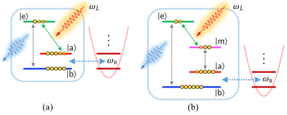
Figure 1: Demonstration for the interaction between a MW resonator mode and (a) a three-level atom, (b) a four-level atom. Here $\omega_{L}$ is the frequency of the driving laser, and $\omega_{\text{{r}}}$ is the frequency of the MW mode. The transition pathways are indicated by the dashed lines.

The dynamics of the composite atom-resonator state $\rho(t)$ is described by the following master equation (interaction picture)

$$\partial_{t}\rho =i[\rho,\,\tilde{V}_{\text{d}}+\tilde{V}_{\text{{ar}}}]+\mathcal{D}_{\text{{a}}}[\rho]+\mathcal{D}_{\text{dep}}[\rho]+\mathcal{D}_{\text{{r}}}[\rho],$$ (1)

$$\mathcal{D}_{\text{{r}}}[\rho] =\kappa\bar{\mathsf{n}}_{\text{{r}}}\big{(}\hat{a}^{{\dagger}}\rho\hat{a}-\tfrac{1}{2}\{\hat{a}\hat{a}^{{\dagger}},\,\rho\}\big{)}$$

$$\qquad+\kappa(\bar{\mathsf{n}}_{\text{{r}}}+1)\big{(}\hat{a}\rho\hat{a}^{{\dagger}}-\tfrac{1}{2}\{\hat{a}^{{\dagger}}\hat{a},\,\rho\}\big{)},$$

$$\mathcal{D}_{\text{{a}}}[\rho] =\sum_{\alpha,\beta}^{\varepsilon_{\alpha}>\varepsilon_{\beta}}\Gamma_{\alpha\beta}^{+}\big{(}\hat{\tau}_{\alpha\beta}^{+}\rho\hat{\tau}_{\alpha\beta}^{-}-\tfrac{1}{2}\{\hat{\tau}_{\alpha\beta}^{-}\hat{\tau}_{\alpha\beta}^{+},\rho\}\big{)}$$

$$\qquad+\Gamma_{\alpha\beta}^{-}\big{(}\hat{\tau}_{\alpha\beta}^{-}\rho\hat{\tau}_{\alpha\beta}^{+}-\tfrac{1}{2}\{\hat{\tau}_{\alpha\beta}^{+}\hat{\tau}_{\alpha\beta}^{-},\rho\}\big{)},$$

$$\mathcal{D}_{\text{dep}}[\rho] =\frac{1}{2}\gamma_{\text{dep}}\big{(}\hat{\sigma}^{z}\rho\hat{\sigma}^{z}-\rho\big{)}.$$

Here, $\mathcal{D}_{\text{{r}}}[\rho]$ and $\mathcal{D}_{\text{{a}}}[\rho]$ describe the dissipation effect of the MW mode and the atom respectively. We denote $\kappa$ as the resonator decay rate, $\Gamma_{\alpha\beta}^{+}:=\gamma_{\alpha\beta}\bar{\mathsf{n}}_{\alpha\beta}$, $\Gamma_{\alpha\beta}^{-}:=\gamma_{\alpha\beta}(\bar{\mathsf{n}}_{\alpha\beta}+1)$ as the dissipation rates of the atom, where $\gamma_{\alpha\beta}$ are the spontaneous decay rates, and $\bar{\mathsf{n}}_{\text{{r}}}:=(e^{\omega_{\text{{r}}}/T}-1)^{-1}$, $\bar{\mathsf{n}}_{\alpha\beta}:=(e^{\Omega_{\alpha\beta}/T}-1)^{-1}$ are the Planck functions with temperature $T$. These dissipation rates satisfy the Boltzmann ratio $\Gamma_{\alpha\beta}^{+}/\Gamma_{\alpha\beta}^{-}=e^{-\Omega_{\alpha\beta}/T}$.

In the atom dissipation term $\mathcal{D}_{\text{{a}}}[\rho]$ we only consider the optical transitions $|\mathsf{e}\rangle\leftrightarrow|\mathsf{a}\rangle$, $|\mathsf{e}\rangle\leftrightarrow|\mathsf{b}\rangle$ [the dashed paths in Fig. 1(a)]. Since $\Omega_{\mathsf{ab}}$ is in the MW regime, generally the spontaneous decay rate between $|\mathsf{a}\rangle$, $|\mathsf{b}\rangle$ is negligibly small. Besides, the pure dephasing effect of $|\mathsf{a}\rangle$, $|\mathsf{b}\rangle$ is taken into account here, which is described by $\mathcal{D}_{\text{dep}}[\rho]$ (denoting $\hat{\sigma}^{z}:=|\mathsf{a}\rangle\langle\mathsf{a}|-|\mathsf{b}\rangle\langle\mathsf{b}|$, and $\gamma_{\text{dep}}$ is the pure dephasing rate).

Such a three level system can be regarded as an SSDG quantum refrigerator (Scovil and Schulz-DuBois, 1959; Geusic et al., 1967; Wang et al., 2015; Cao et al., 2022). A driving laser is applied on $|\mathsf{a}\rangle\leftrightarrow|\mathsf{e}\rangle$, making the population on $|\mathsf{a}\rangle$ greatly reduced and approach zero, and then the “heat” is dumped away through the optical emission $|\mathsf{e}\rangle\rightarrow|\mathsf{b}\rangle$. Effectively, that makes the three-level atom become a system with zero temperature, which could absorb “heat” from the MW resonator. By this way the thermal photons in the MW resonator can be continuously reduced by the quantum refrigerator.

MW mode dynamics - To give a more precise description for the above cooling process, we need a dynamical equation solely for the resonator state $\varrho_{\text{{r}}}\equiv\mathrm{tr}_{\text{{a}}}\rho$. Generally speaking, the atom could achieve its steady state much faster than the resonator mode. That enables us to apply the adiabatic elimination (Cirac et al., 1992; Scully and Zubairy, 1997; Gardiner and Zoller, 2004), which finally gives an equation for the MW mode alone, that is (see Appendix A),

$$\partial_{t}\varrho_{\text{{r}}}= (A_{+}+\kappa\bar{\mathsf{n}}_{\text{{r}}})\big{(}\hat{a}^{\dagger}\varrho_{\text{{r}}}\hat{a}-\tfrac{1}{2}\{\varrho_{\text{{r}}},\,\hat{a}^{\dagger}\hat{a}\}\big{)}$$

$$+[A_{-}+\kappa(\bar{\mathsf{n}}_{\text{{r}}}+1)]\big{(}\hat{a}\varrho_{\text{{r}}}\hat{a}^{{\dagger}}-\tfrac{1}{2}\{\varrho_{\text{{r}}},\,\hat{a}\hat{a}^{\dagger}\}\big{)}.$$ (2)

Here, $A_{-(+)}$ can be regarded as the cooling (heating) rate induced by the atom, and they are given by

$$A_{\pm}:=2g^{2}\,\mathrm{Re}\int_{0}^{\infty}ds\,\langle\hat{\sigma}^{\pm}(s)\hat{\sigma}^{\mp}(0)\rangle_{\text{ss}}.$$ (3)

Here $\langle\hat{\sigma}^{\pm}(s)\hat{\sigma}^{\mp}(0)\rangle_{\text{ss}}$ is the time correlation function of the atom in the steady state when it is not coupled with the MW resonator, which is described by ($\varrho_{\text{{a}}}\equiv\mathrm{tr}_{\text{{r}}}\rho$ is the atom state)

$$\partial_{t}\varrho_{\text{{a}}}=i[\varrho_{\text{{a}}},\,\tilde{V}_{\text{d}}]+\mathcal{D}_{\text{{a}}}[\varrho_{\text{{a}}}]+\mathcal{D}_{\text{dep}}[\varrho_{\text{{a}}}].$$ (4)

In the steady state $t\rightarrow\infty$, the above resonator equation (2) gives the MW photon number as

$$\langle\hat{n}\rangle_{\text{ss}}=\frac{A_{+}+\kappa\bar{\mathsf{n}}_{\text{{r}}}}{A_{-}-A_{+}+\kappa}.$$ (5)

If the cooling rate is fast enough ($A_{-}\gg A_{+},\,\kappa\bar{\mathsf{n}}_{\text{{r}}}$), we obtain $\langle\hat{n}\rangle_{\text{ss}}\rightarrow 0$, which means the thermal noise in the MW resonator is greatly suppressed.

The time correlation functions $\langle\hat{\sigma}^{\pm}(s)\hat{\sigma}^{\mp}(0)\rangle_{\text{ss}}$ in $A_{\pm}$ can be calculated with the help of the quantum regression theorem from the atom equation (4) (Scully and Zubairy, 1997; Gardiner and Zoller, 2004; Agarwal, 2012; Breuer and Petruccione, 2002). For the three level system [Fig. 1(a)], that gives the heating and cooling rates (3) as (the full results are presented in Appendix B)

$$A_{+} =\frac{2g^{2}}{\bar{\Upsilon}_{\mathsf{ab}}+\tilde{\Omega}_{\text{d}}^{2}/4\bar{\Upsilon}_{\mathsf{eb}}}\mathrm{Re}\big{[}\langle\hat{\text{{n}}}_{\mathsf{a}}\rangle_{\text{ss}}+\frac{i\tilde{\Omega}_{\text{d}}}{2\bar{\Upsilon}_{\mathsf{eb}}}\langle\hat{\tau}_{\mathsf{ea}}^{+}\rangle_{\text{ss}}\big{]},$$

$$A_{-} =\frac{2g^{2}}{\bar{\Upsilon}_{\mathsf{ab}}+\tilde{\Omega}_{\text{d}}^{2}/4\bar{\Upsilon}_{\mathsf{eb}}}\langle\hat{\text{{n}}}_{\mathsf{b}}\rangle_{\text{ss}},$$ (6)

where $\bar{\Upsilon}_{\mathsf{ab}}:=\gamma_{\text{dep}}+\frac{1}{2}(\Gamma_{\mathsf{ea}}^{+}+\Gamma_{\mathsf{eb}}^{+})$, $\bar{\Upsilon}_{\mathsf{eb}}:=\frac{1}{2}(\gamma_{\text{dep}}+\Gamma_{\mathsf{ea}}^{-}+\Gamma_{\mathsf{eb}}^{-}+\Gamma_{\mathsf{eb}}^{+})$ are constants. $\langle\hat{\text{{n}}}_{\mathsf{a(b)}}\rangle_{\text{ss}}$ is the steady state population on $|\mathsf{a(b)}\rangle$, $\langle\hat{\tau}_{\mathsf{ea}}^{+}\rangle_{\text{ss}}$ is the coherence term, which can be solved by the atom equation (4), and they give

$$\frac{\langle\hat{\text{{n}}}_{\mathsf{a}}\rangle_{\text{ss}}}{\langle\hat{\text{{n}}}_{\mathsf{b}}\rangle_{\text{ss}}} =\frac{\Gamma_{\mathsf{eb}}^{+}}{\Gamma_{\mathsf{eb}}^{-}}\cdot\frac{\Gamma_{\mathsf{ea}}^{-}+\tilde{\Omega}_{\text{d}}^{2}/(\Gamma_{\mathsf{ea}}^{+}+\Gamma_{\mathsf{ea}}^{-}+\Gamma_{\mathsf{eb}}^{-})}{\Gamma_{\mathsf{ea}}^{+}+\tilde{\Omega}_{\text{d}}^{2}/(\Gamma_{\mathsf{ea}}^{+}+\Gamma_{\mathsf{ea}}^{-}+\Gamma_{\mathsf{eb}}^{-})},$$

$$\frac{\langle\hat{\text{{n}}}_{\mathsf{e}}\rangle_{\text{ss}}}{\langle\hat{\text{{n}}}_{\mathsf{b}}\rangle_{\text{ss}}} =e^{-\Omega_{\mathsf{eb}}/T},\quad\langle\hat{\tau}_{\mathsf{ea}}^{-}\rangle_{\text{ss}}=\frac{i\tilde{\Omega}_{\text{d}}\big{(}\langle\hat{\text{{n}}}_{\mathsf{e}}\rangle-\langle\hat{\text{{n}}}_{\mathsf{a}}\rangle\big{)}}{\Gamma_{\mathsf{ea}}^{+}+\Gamma_{\mathsf{ea}}^{-}+\Gamma_{\mathsf{eb}}^{-}}.$$ (7)

When the driving strength $\tilde{\Omega}_{\text{d}}$ is strong enough, the above ratios give $\langle\hat{\text{{n}}}_{\mathsf{a}}\rangle_{\text{ss}}/\langle\hat{\text{{n}}}_{\mathsf{b}}\rangle_{\text{ss}}\rightarrow e^{-\Omega_{\mathsf{eb}}/T}\simeq 0$ (for the optical frequency $\Omega_{\mathsf{eb}}\gg T\simeq 300\,\text{K}$), namely, $\langle\hat{\text{{n}}}_{\mathsf{b}}\rangle_{\text{ss}}\simeq 1$ and $\langle\hat{\text{{n}}}_{\mathsf{a,e}}\rangle_{\text{ss}}\simeq\langle\hat{\tau}_{\mathsf{ea}}^{-}\rangle_{\text{ss}}\simeq 0$ (see details in Appendix B). That means, the population is fully concentrated in the ground state $|\mathsf{b}\rangle$. As mentioned above, such a population distribution effectively gives a zero temperature $T_{\mathsf{ab}}^{\text{eff}}\rightarrow 0$.

On the first sight, to achieve a better cooling effect, a stronger driving strength might be preferred, since that would make the populations more concentrated into the ground state $|\mathsf{b}\rangle$, leading to $T_{\mathsf{ab}}^{\text{eff}}\rightarrow 0$. However, it is worth noting that the driving strength $\tilde{\Omega}_{\text{d}}$ also appears in the correction factor $2g^{2}/(\bar{\Upsilon}_{\mathsf{ab}}+\tilde{\Omega}_{\text{d}}^{2}/4\bar{\Upsilon}_{\mathsf{eb}})$ in the cooling/heating rates $A_{\pm}$ [Eq. (6)]. As a result, when the driving strength $\tilde{\Omega}_{\text{d}}$ is too large, both the cooling and heating rates decrease towards zero $A_{\pm}\rightarrow 0$, and that greatly weakens the cooling effect.

The reason can be understood by the following picture. For the two levels $|\mathsf{e}\rangle$ and $|\mathsf{a}\rangle$ under the laser driving, effectively the driving field also perturbs these two levels, which makes them shift upwards and downwards. As a result, the energy gap of the lowest two levels would also be changed correspondingly due to the energy shift of $|\mathsf{a}\rangle$, and that makes the energy gap $\Omega_{\mathsf{ab}}$ no longer resonant with the resonator frequency $\omega_{\text{{r}}}$. Because of such an off-resonant coupling, the energy cannot be efficiently transported from the MW resonator to the atom refrigerator, and thus the cooling and heating rates are both weakened.

Four-level improvement - To overcome the above weakening problem of the cooling rate induced by the driving field perturbation, here we consider using a four-level system as the refrigerator to improve the cooling performance (Wang et al., 2015; Li et al., 2017).

In this setup [Fig. 1(b)], still the lowest two levels $|\mathsf{a,b}\rangle$ are resonantly coupled with the MW resonator, while a mediated level $|\mathsf{m}\rangle$ is added between $|\mathsf{e}\rangle$ and $|\mathsf{a}\rangle$ (assuming $\Omega_{\mathsf{em}},\,\Omega_{\mathsf{ma}}$ are in the optical frequency regime), and now the driving laser is applied to the transition $|\mathsf{e}\rangle\leftrightarrow|\mathsf{m}\rangle$, which would no longer perturb $|\mathsf{a,b}\rangle$ directly. Similarly as the above three-level case, only the optical transitions $|\mathsf{e}\rangle\leftrightarrow|\mathsf{m}\rangle$, $|\mathsf{m}\rangle\leftrightarrow|\mathsf{a}\rangle$, and $|\mathsf{e}\rangle\leftrightarrow|\mathsf{b}\rangle$ are considered [the dashed paths in Fig. 1(b)]; the transition between $|\mathsf{a}\rangle$ and $|\mathsf{b}\rangle$ is neglected, while their dephasing effect is considered.

In this case, the driving laser moves the population from $|\mathsf{m}\rangle$ to $|\mathsf{e}\rangle$, and the “heat” could be dumped out through the optical emission $|\mathsf{e}\rangle\rightarrow|\mathsf{b}\rangle$; meanwhile, the population decrease in $|\mathsf{m}\rangle$ would be complemented from $|\mathsf{a}\rangle$ through the thermal excitation $|\mathsf{m}\rangle\leftrightarrow|\mathsf{a}\rangle$, until their populations satisfy the Boltzmann distribution. This is similar as a thermally “siphonic” effect. As a result, under a strong enough driving intensity, the atom population could be fully concentrated into the ground state $|\mathsf{b}\rangle$, meanwhile, the energy gap $\Omega_{\mathsf{ab}}$ would no longer be perturbed and still keep resonant with the MW resonator ($\Omega_{\mathsf{ab}}=\omega_{\text{{r}}}$).

Intuitively, the population in $|\mathsf{m}\rangle$ is almost zero, which makes the driving laser seem being applied on “nothing”. But in a finite temperature $T$, there still remains a nonzero population, though quite small. It turns out this is enough to achieve the above “siphonic” cooling process.

For this four-level system, we still apply the adiabatic elimination to derive the equation for the MW mode alone, and it turns out to have the same form as the above resonator equation (2) for the three-level case. And the heating and cooling rates $A_{\pm}^{\prime}$ are still defined by Eq. (3), except now the correlation functions $\langle\hat{\sigma}^{\pm}(s)\hat{\sigma}^{\mp}(0)\rangle_{\text{ss}}$ in $A_{\pm}^{\prime}$ [Eq. (3)] should be calculated from the four-level system under the laser driving. With the help of the quantum regression theorem, for this four-level setup, the heating and cooling rates are obtained as (the full results are presented in Appendix C)

$$A_{+}^{\prime}=\frac{2g^{2}}{\bar{\Upsilon}_{\mathsf{ab}}^{\prime}}\langle\hat{\text{{n}}}_{\mathsf{a}}\rangle_{\text{ss}},\qquad A_{-}^{\prime}=\frac{2g^{2}}{\bar{\Upsilon}_{\mathsf{ab}}^{\prime}}\langle\hat{\text{{n}}}_{\mathsf{b}}\rangle_{\text{ss}},$$ (8)

where $\bar{\Upsilon}_{\mathsf{ab}}^{\prime}:=\gamma_{\text{dep}}+\frac{1}{2}(\Gamma_{\mathsf{eb}}^{+}+\Gamma_{\mathsf{ma}}^{+})$ is a decay rate constant. In the steady state, the population ratios in this four-level system satisfy (Appendix C)

$$\frac{\langle\hat{\text{{n}}}_{\mathsf{m}}\rangle_{\text{ss}}}{\langle\hat{\text{{n}}}_{\mathsf{a}}\rangle_{\text{ss}}} =e^{-\Omega_{\mathsf{ma}}/T},\qquad\frac{\langle\hat{\text{{n}}}_{\mathsf{e}}\rangle_{\text{ss}}}{\langle\hat{\text{{n}}}_{\mathsf{b}}\rangle_{\text{ss}}}=e^{-\Omega_{\mathsf{eb}}/T},$$

$$\frac{\langle\hat{\text{{n}}}_{\mathsf{e}}\rangle_{\text{ss}}}{\langle\hat{\text{{n}}}_{\mathsf{m}}\rangle_{\text{ss}}} =\frac{\Gamma_{\mathsf{em}}^{+}+\tilde{\Omega}_{\text{d}}^{2}/(\Gamma_{\mathsf{em}}^{+}+\Gamma_{\mathsf{em}}^{-}+\Gamma_{\mathsf{eb}}^{-}+\Gamma_{\mathsf{ma}}^{-})}{\Gamma_{\mathsf{em}}^{-}+\tilde{\Omega}_{\text{d}}^{2}/(\Gamma_{\mathsf{em}}^{+}+\Gamma_{\mathsf{em}}^{-}+\Gamma_{\mathsf{eb}}^{-}+\Gamma_{\mathsf{ma}}^{-})}.$$ (9)

When the driving strength $\tilde{\Omega}_{\text{d}}\rightarrow\infty$, the ratios (9) give $\langle\hat{\text{{n}}}_{\mathsf{e}}\rangle_{\text{ss}}/\langle\hat{\text{{n}}}_{\mathsf{m}}\rangle_{\text{ss}}\simeq 1$, and $\langle\hat{\text{{n}}}_{\mathsf{a}}\rangle_{\text{ss}}/\langle\hat{\text{{n}}}_{\mathsf{b}}\rangle_{\text{ss}}\simeq e^{-(\Omega_{\mathsf{eb}}-\Omega_{\mathsf{ma}})/T}\rightarrow 0$. That indicates the populations could be fully concentrated into the ground state, i.e., $\langle\hat{\text{{n}}}_{\mathsf{b}}\rangle_{\text{ss}}\rightarrow 1$, $\langle\hat{\text{{n}}}_{\mathsf{a}}\rangle_{\text{ss}}\rightarrow 0$, which also gives $T_{\mathsf{ab}}^{\text{eff}}\rightarrow 0$.

More importantly, unlike the above three-level case [Eq. (6)], now the driving strength $\tilde{\Omega}_{\text{d}}$ no longer appears in the correction factor $2g^{2}/\bar{\Upsilon}_{\mathsf{ab}}^{\prime}$ in $A_{\pm}^{\prime}$ [Eq. (8)]. Thus, with the increase of the driving light intensity, here the cooling (heating) rate increases (decreases) monotonically. Therefore, when the driving strength $\tilde{\Omega}_{\text{d}}\rightarrow\infty$, the cooling performance could achieve the optimum, and that gives $A_{+}^{\prime}\rightarrow 0$ and $A_{-}^{\prime}\rightarrow 2g^{2}/\bar{\Upsilon}_{\mathsf{ab}}^{\prime}$.

All the above discussions are based on the interaction between the MW resonator and a single multi-level system. Generally, the coupling strength $g$ between an MW resonator mode and a single atom is quite small. This can be improved by adopting $N$ atom refrigerators to couple with the resonator. Correspondingly, the above cooling and heating rates $A_{\pm}$ obtained from a single refrigerator can be enlarged by $N$ times. Effectively, this also can be regarded as the enlargement in the coupling strength, $g\mapsto g_{N}\equiv\sqrt{N}\,g$, which is similar as the treatment in lasing problems (Scully and Zubairy, 1997; Breuer and Petruccione, 2002; Agarwal, 2012).

Based on the above results, the cooling limit of the photon number in the MW resonator [Eq. (5)] is obtained as

$$\langle\hat{n}\rangle_{\text{ss}}\stackrel{{\scriptstyle\tilde{\Omega}_{\text{d}}\rightarrow\infty}}{{\longrightarrow}}\frac{\kappa\bar{\mathsf{n}}_{\text{{r}}}}{2g_{N}^{2}/\bar{\Upsilon}_{\mathsf{ab}}^{\prime}+\kappa}\simeq\bar{\mathsf{n}}_{\text{{r}}}\big{/}\frac{2g_{N}^{2}}{\kappa\gamma_{\text{dep}}}.$$ (10)

Here, in the decay rate $\bar{\Upsilon}_{\mathsf{ab}}^{\prime}$ [see the definition under Eq. (8)], $\Gamma_{\mathsf{eb}}^{+}\equiv\gamma_{\mathsf{eb}}\,\bar{\mathsf{n}}_{\mathsf{eb}}\simeq 0$, $\Gamma_{\mathsf{ma}}^{+}\equiv\gamma_{\mathsf{ma}}\,\bar{\mathsf{n}}_{\mathsf{ma}}\simeq 0$ (since $\Omega_{\mathsf{eb}},\Omega_{\mathsf{ma}}\gg T$), thus generally the dephasing rate gives the main contribution, i.e., $\bar{\Upsilon}_{\mathsf{ab}}^{\prime}\simeq\gamma_{\text{dep}}$. Therefore, to achieve a better cooling effect, we need $Ng^{2}/\kappa\gamma_{\text{dep}}\gg 1$, which requires a stronger coupling strength $g_{N}\equiv\sqrt{N}\,g$, a smaller resonator loss $\kappa$, and a smaller dephasing rate $\gamma_{\text{dep}}$.

Experiment estimation - Now we make an estimation for the possible cooling limit in realistic experiments. For the example of an MW resonator with $\omega_{\text{{r}}}/2\pi=1\,\text{GHz}$, at room temperature $T=300\,\text{K}$, the thermal photon number from the surrounding reservoir is $\bar{\mathsf{n}}_{\text{{r}}}\simeq 6.2\times 10^{3}$. A quality factor $Q\simeq 10^{4}$ is an achievable estimation, which gives the resonator decay rate as $\kappa/2\pi\simeq 0.1\,\text{MHz}$ (Breeze et al., 2017; Wu et al., 2021; Day et al., 2024).

The multi-level systems can be implemented by the defect structures in solid crystals (e.g., NV or SiV centers in diamonds or silicon carbide (Fischer et al., 2018; Gottscholl et al., 2023; Castelletto et al., 2024), pentacene molecules doped in the p-terphenyl crystal (Wu et al., 2021, 2022a)), or certain atoms in the form of gas, or doped in solid crystals, which is similar as the gas or solid laser systems. It is reported that the effective coupling strength between the MW resonator and NV ensemble could achieve $g_{N}/2\pi\simeq 1.5\,\text{MHz}$ (Day et al., 2024). For the dephasing rate, a typical estimation is $\gamma_{\text{dep}}/2\pi\simeq 0.5\,\text{MHz}$, which corresponds to $T_{2}^{*}\simeq 2\,\mu\text{s}$ (Liu et al., 2012; Zhang et al., 2024; Breeze et al., 2017).

Based on the above experimental parameters, the cooling limit (10) gives the steady photon number in the MW resonator as $\langle\hat{n}\rangle_{\text{ss}}\simeq 69$, which corresponds to an effective temperature $T_{\text{{r}}}^{\text{eff}}\equiv\hbar\omega_{\text{{r}}}\big{/}k_{\text{{b}}}\ln(1+1/\langle\hat{n}\rangle_{\text{ss}})\simeq 3.3\,\text{K}$ (starting from room temperature). Such a cooling effect is well comparable with the liquid helium temperature. It is possible to achieve a better result if a stronger coupling strength or smaller dephasing rate could be adopted (Kato et al., 2023).

Summary - In this paper, we consider using three-level or four-level atoms as quantum refrigerators to cool down an MW resonator, and investigate the possible cooling limits. Under proper transition structures, a laser pump drives the atom to work as an SSDG quantum refrigerator, and the atom population is fully concentrated into the ground state, effectively giving a zero temperature. Then the thermal photons in the MW resonator can be continuously absorbed away by the atom.

By adopting the adiabatic elimination, we obtain a master equation for the resonator mode, which gives a more precise description for this cooling system. We find that, though the atom can be well cooled down, the laser driving also significantly perturbs the atom levels. Such perturbation may cause the atom-resonator coupling to become off-resonant, which prevents the heat transport from the MW resonator to the refrigerator, and that greatly weakens the cooling effect. We find that this issue can be well overcome by adopting four-level systems as the refrigerators. Based on some practical parameters, our estimation shows the cooling limit of the MW resonator could reach the liquid helium temperature ($T_{\text{{r}}}^{\text{eff}}\simeq 3.3\,\text{K}$ for $\omega_{\text{{r}}}/2\pi=1\,\text{GHz}$). Our results highlight the potential of quantum refrigerators as practical, high-performance solutions for suppressing thermal noise in MW devices without cryogenic complexity (Scully et al., 2003; Quan et al., 2005, 2006; Kosloff, 2013; Uzdin et al., 2015).

Acknowledgments - SWL appreciates quite much for the helpful discussion with H. Wu and B. Zhang in BIT. This study is supported by NSF of China (Grant No. 12475030).

Appendix A The master equation for the MW resonator alone

Here we show the derivation of the master equation which describes the resonator mode alone. In the interaction picture (applied by $\hat{H}_{\text{{a}}}+\hat{H}_{\text{{r}}}$), we rewrite the equation for the atom-resonator system as $\partial_{t}\rho=(\mathcal{L}_{\text{{a}}}+\mathcal{K}_{\text{{ar}}}+\mathcal{D}_{\text{{r}}})[\rho]$, where

$$\mathcal{L}_{\text{{a}}}[\rho] =i[\rho,\,\tilde{V}_{\text{d}}]+\mathcal{D}_{\text{{a}}}[\rho]+\mathcal{D}_{\text{dep}}[\rho],$$

$$\mathcal{K}_{\text{{ar}}}[\rho] =i[\rho,\,\tilde{V}_{\text{{ar}}}]=i\,[\rho,\,g(\hat{\sigma}^{+}\hat{a}+\hat{\sigma}^{-}\hat{a}^{{\dagger}})].$$ (11)

Here $\mathcal{D}_{\text{{r}}}[\rho]$ describes the dissipation of the resonator mode, $\mathcal{L}_{\text{{a}}}[\rho]$ describes the atom dissipation together with the laser driving $\tilde{V}_{\text{d}}$, and $\mathcal{K}_{\text{{ar}}}[\rho]$ describes the interaction between the atom and the resonator.

Here we need a dynamical equation solely for the resonator state $\varrho_{\text{{r}}}=\mathrm{tr}_{\text{{a}}}\rho$. Generally, the dissipation rate of the MW resonator is much slower than that of the atom, and $\mathcal{D}_{\text{{r}}}[\rho]$ simply gives $\mathrm{tr}_{\text{{a}}}\big{\{}\mathcal{D}_{\text{{r}}}[\rho]\big{\}}=\mathcal{D}_{\text{{r}}}[\varrho_{\text{{r}}}]$, therefore, in the following discussions we first omit this term and then take it back in the final step.

The master equation $\partial_{t}\rho=(\mathcal{L}_{\text{{a}}}+\mathcal{K}_{\text{{ar}}})[\rho]$ has a similar linear structure with the Schrödinger equation, thus we treat $\mathcal{K}_{\text{{ar}}}$ as a perturbation based on $\mathcal{L}_{\text{{a}}}$. The steady states of $\mathcal{L}_{\text{{a}}}[\rho]=0$ form a degenerated subspace, i.e., $\mathcal{L}_{\text{{a}}}\left[\ |n\rangle\langle n|\otimes\varrho_{\text{{a}}}^{\text{ss}}\ \right]=0$, where $|n\rangle$ are the Fock states for the MW mode, and $\varrho_{\text{{a}}}^{\text{ss}}$ is the steady state of the atom ($\mathcal{L}_{\text{{a}}}[\varrho_{\text{{a}}}^{\text{ss}}]=0$). Thus, the degenerated perturbation can be applied based on this subspace (Takahashi, 1977; Wu et al., 2022b). Here we introduce some projection operators $\mathcal{P}[\rho]:=\mathcal{P}_{\text{{r}}}\cdot\mathcal{P}_{\text{{a}}}[\rho]$, where

$$\mathcal{P}_{\text{{r}}}[\rho] :=\sum_{n=0}^{\infty}\langle n|\rho|n\rangle\ |n\rangle\langle n|,\qquad\mathcal{P}_{\text{{a}}}[\rho]:=\lim_{t\rightarrow\infty}e^{t\mathcal{L}_{\text{{a}}}}[\rho]=\varrho_{\text{{a}}}^{\text{ss}}\otimes\mathrm{tr}_{\text{{a}}}[\rho].$$ (12)

Such a projection gives $\mathcal{P}[\rho(t)]=\varrho_{\text{{a}}}^{\text{ss}}\otimes\mu(t)$, where $\mu(t)\equiv\sum p_{n}(t)\,|n\rangle\langle n|$ is the diagonal part of the resonator state $\varrho_{\text{{r}}}(t)$. Then effectively the above master equation can be described by (Takahashi, 1977; Wu et al., 2022b; Cirac et al., 1992; Gardiner and Zoller, 2004)

$$\partial_{t}\mathcal{P}[\rho] =\mathcal{P}\mathcal{K}_{\text{{ar}}}(-\mathcal{L}_{\text{{a}}})^{-1}\mathcal{K}_{\text{{ar}}}\mathcal{P}\,[\rho],$$

$$\Rightarrow\quad\partial_{t}\mu =\mathcal{P}_{\text{{r}}}\ \mathrm{tr}_{\text{{a}}}\Big{\{}\mathcal{P}_{\text{{a}}}\ \mathcal{K}_{\text{{ar}}}(-\mathcal{L}_{\text{{a}}})^{-1}\mathcal{K}_{\text{{ar}}}\mathcal{P}[\rho]\Big{\}}=\mathcal{P}_{\text{{r}}}\int_{0}^{\infty}ds\,\mathrm{tr}_{\text{{a}}}\Big{\{}\mathcal{K}_{\text{{ar}}}\,e^{s\mathcal{L}_{\text{{a}}}}\mathcal{K}_{\text{{ar}}}\,\mathcal{P}[\rho(t)]\Big{\}}.$$ (13)

In the last equation, the super operator $\mathcal{L}_{\text{{a}}}^{-1}$ is formally replaced by its Laplacian integral, and the integration term has been simplified by $\mathrm{tr}_{\text{{a}}}\big{\{}\mathcal{P}_{\text{{a}}}\ \mathcal{L}[\rho]\big{\}}=\mathrm{tr}_{\text{{a}}}\big{\{}\,\varrho_{\text{{a}}}^{\text{ss}}\otimes\mathrm{tr}_{\text{{a}}}(\mathcal{L}[\rho])\,\big{\}}=\mathrm{tr}_{\text{{a}}}\big{\{}\mathcal{L}[\rho]\big{\}}$.

Further, denoting $\Theta_{s}:=e^{s\mathcal{L}_{\text{{a}}}}\mathcal{K}_{\text{{ar}}}\mathcal{P}[\rho]$ for short, the above integration term becomes $\mathrm{tr}_{\text{{a}}}\big{\{}\mathcal{K}_{\text{{ar}}}[\Theta_{s}]\big{\}}=ig\ [\,\mathrm{tr}_{\text{{a}}}(\hat{\sigma}^{+}\Theta_{s}),\,\hat{a}\,]+ig\ [\,\mathrm{tr}_{\text{{a}}}(\hat{\sigma}^{-}\Theta_{s}),\,\hat{a}^{{\dagger}}\,]$ (using the relation $\mathrm{tr}_{\text{{a}}}\big{\{}\,[\Theta_{s},\,\hat{X}_{\text{{a}}}\cdot\hat{Y}_{\text{{r}}}]\,\big{\}}=[\,\mathrm{tr}_{\text{{a}}}(\hat{X}_{\text{{a}}}\Theta_{s}),\,\hat{Y}_{\text{{r}}}\,]$). That further gives

$$\mathrm{tr}_{\text{{a}}}(\hat{\sigma}^{+}\Theta_{s}) =\mathrm{tr}_{\text{{a}}}\big{\{}\hat{\sigma}^{+}\cdot e^{s\mathcal{L}_{\text{{a}}}}\ \mathcal{K}_{\text{{ar}}}[\mathcal{P}\rho]\big{\}}=ig\ \mathrm{tr}_{\text{{a}}}\Big{\{}\hat{\sigma}^{+}(s)\cdot[\varrho_{\text{{a}}}^{\text{ss}}\cdot\mu_{t},\,\hat{\sigma}^{+}\hat{a}+\hat{\sigma}^{-}\hat{a}^{{\dagger}}]\Big{\}}$$

$$=ig\ \Big{\{}\langle\hat{\sigma}^{+}(0)\hat{\sigma}^{+}(s)\rangle_{\text{ss}}\>\mu_{t}\hat{a}+\langle\hat{\sigma}^{-}(0)\hat{\sigma}^{+}(s)\rangle_{\text{ss}}\>\mu_{t}\hat{a}^{{\dagger}}-\langle\hat{\sigma}^{+}(s)\hat{\sigma}^{+}(0)\rangle_{\text{ss}}\>\hat{a}\mu_{t}-\langle\hat{\sigma}^{+}(s)\hat{\sigma}^{-}(0)\rangle_{\text{ss}}\>\hat{a}^{{\dagger}}\mu_{t}\Big{\}},$$ (14)

$$\mathrm{tr}_{\text{{a}}}(\hat{\sigma}^{-}\Theta_{s}) =ig\ \Big{\{}\langle\hat{\sigma}^{+}(0)\hat{\sigma}^{-}(s)\rangle_{\text{ss}}\>\mu_{t}\hat{a}+\langle\hat{\sigma}^{-}(0)\hat{\sigma}^{-}(s)\rangle_{\text{ss}}\>\mu_{t}\hat{a}^{{\dagger}}-\langle\hat{\sigma}^{-}(s)\hat{\sigma}^{+}(0)\rangle_{\text{ss}}\>\hat{a}\mu_{t}-\langle\hat{\sigma}^{-}(s)\hat{\sigma}^{-}(0)\rangle_{\text{ss}}\>\hat{a}^{{\dagger}}\mu_{t}\Big{\}}.$$

Taking these results back to the above Eq. (13), we obtain

$$\partial_{t}\mu= ig\,\mathcal{P}_{\text{{r}}}\int_{0}^{\infty}ds\ \Big{\{}[\mathrm{tr}_{\text{a}}(\hat{\sigma}^{+}\Theta_{s}),\,\hat{a}]+[\mathrm{tr}_{\text{a}}(\hat{\sigma}^{-}\Theta_{s}),\,\hat{a}^{{\dagger}}]\Big{\}}$$

$$= -g^{2}\int_{0}^{\infty}ds\ \Big{\{}\langle\hat{\sigma}^{-}(0)\hat{\sigma}^{+}(s)\rangle_{\text{ss}}\,[\mu_{t}\hat{a}^{{\dagger}},\,\hat{a}]-\langle\hat{\sigma}^{+}(s)\hat{\sigma}^{-}(0)\rangle_{\text{ss}}\>[\hat{a}^{{\dagger}}\mu_{t},\,\hat{a}]$$

$$\quad\qquad\qquad+\langle\hat{\sigma}^{+}(0)\hat{\sigma}^{-}(s)\rangle_{\text{ss}}\>[\mu_{t}\hat{a},\,\hat{a}^{{\dagger}}]-\langle\hat{\sigma}^{-}(s)\hat{\sigma}^{+}(0)\rangle_{\text{ss}}\>[\hat{a}\mu_{t},\,\hat{a}^{{\dagger}}]\Big{\}},$$ (15)

where the double annihilation/creation terms are dropped due to the projection operation $\mathcal{P}_{\text{{r}}}$. Since $\left(\langle\hat{\sigma}^{\pm}(0)\hat{\sigma}^{\mp}(s)\rangle_{\text{ss}}\right)^{*}=\langle\hat{\sigma}^{\pm}(s)\hat{\sigma}^{\mp}(0)\rangle_{\text{ss}}$, the above equation also can be written as

$$\partial_{t}\mu =\frac{1}{2}A_{+}\big{(}[\hat{a}^{{\dagger}}\mu,\hat{a}]+\mathrm{H.c.}\big{)}+\frac{1}{2}A_{-}\big{(}[\hat{a}\mu,\hat{a}^{{\dagger}}]+\mathrm{H.c.}\big{)},$$

$$A_{+} :=2g^{2}\,\mathrm{Re}\int_{0}^{\infty}ds\,\langle\hat{\sigma}^{+}(s)\hat{\sigma}^{-}(0)\rangle_{\text{ss}},\qquad A_{-}:=2g^{2}\,\mathrm{Re}\int_{0}^{\infty}ds\,\langle\hat{\sigma}^{-}(s)\hat{\sigma}^{+}(0)\rangle_{\text{ss}}.$$ (16)

Now taking back the original dissipation term $\mathcal{D}_{\text{{r}}}[\rho]$, we obtain the master equation solely for the MW resonator, i.e.,

$$\partial_{t}\mu =\Gamma_{+}\big{(}\hat{a}^{\dagger}\mu\hat{a}-\frac{1}{2}\{\mu,\,\hat{a}^{\dagger}\hat{a}\}\big{)}+\Gamma_{-}\big{(}\hat{a}\mu\hat{a}^{{\dagger}}-\frac{1}{2}\{\mu,\,\hat{a}\hat{a}^{\dagger}\}\big{)},$$ (17)

$$\Gamma_{+} =A_{+}+\kappa\bar{\mathsf{n}}_{\text{{r}}},\qquad\Gamma_{-}=A_{-}+\kappa(\bar{\mathsf{n}}_{\text{{r}}}+1).$$

Here $\Gamma_{+\,(-)}$ indicates the increasing (decreasing) rate of the photon number of the resonator, and $A_{+\,(-)}$ can be regarded as the heating (cooling) rate induced by the atom. In the steady state $t\rightarrow\infty$, that gives the MW photon number as

$$\langle\hat{n}\rangle_{\text{ss}}=\frac{\Gamma_{+}}{\Gamma_{-}-\Gamma_{+}}=\frac{A_{+}+\kappa\bar{\mathsf{n}}_{\text{{r}}}}{A_{-}-A_{+}+\kappa}.$$ (18)

If the cooling rate is fast enough ($A_{-}\gg A_{+},\kappa\bar{\mathsf{n}}_{\text{{r}}}$), the MW photon number becomes $\langle\hat{n}\rangle_{\text{ss}}\rightarrow 0$, which means the thermal noise in the resonator can be greatly suppressed.

The above derivations for the cooling and heating rates are based on the interaction between the MW mode and a single atom. A large number of $N$ atoms can be placed in the MW resonator and used to absorb the thermal photons together. In this case, the cooling and heating rates can be enlarged by $N$ times ($A_{\pm}\mapsto NA_{\pm}$), or equivalently, the atom-resonator coupling strength $g$ can be regarded as enlarged by $\sqrt{N}$ times ($g\mapsto g_{N}:=\sqrt{N}\,g$).

Appendix B The three level system under driving

B.1 Steady state expectations

Here we study the behavior of the three level system when there is no interaction with the resonator. A driving laser is applied to the transition path $|\mathsf{e}\rangle\leftrightarrow|\mathsf{a}\rangle$, and the atom dynamics is described by the master equation (interaction picture)

$$\partial_{t}\varrho_{\text{{a}}} =i[\varrho_{\text{{a}}},\,\frac{1}{2}\tilde{\Omega}_{\text{d}}(\hat{\tau}_{\mathsf{ea}}^{+}+\hat{\tau}_{\mathsf{ea}}^{-})]+\mathcal{D}_{\text{{a}}}[\varrho_{\text{{a}}}]+\mathcal{D}_{\text{dep}}[\varrho_{\text{{a}}}],$$ (19)

$$\mathcal{D}_{\text{{a}}}[\varrho_{\text{{a}}}] =\sum_{\alpha,\beta}^{\varepsilon_{\alpha}>\varepsilon_{\beta}}\Gamma_{\alpha\beta}^{+}\big{(}\hat{\tau}_{\alpha\beta}^{+}\varrho_{\text{{a}}}\hat{\tau}_{\alpha\beta}^{-}-\frac{1}{2}\{\hat{\tau}_{\alpha\beta}^{-}\hat{\tau}_{\alpha\beta}^{+},\,\varrho_{\text{{a}}}\}\big{)}+\Gamma_{\alpha\beta}^{-}\big{(}\hat{\tau}_{\alpha\beta}^{-}\varrho_{\text{{a}}}\hat{\tau}_{\alpha\beta}^{+}-\frac{1}{2}\{\hat{\tau}_{\alpha\beta}^{+}\hat{\tau}_{\alpha\beta}^{-},\,\varrho_{\text{{a}}}\}\big{)},$$

$$\mathcal{D}_{\text{dep}}[\varrho_{\text{{a}}}] =\frac{1}{2}\gamma_{\text{dep}}\big{(}\hat{\sigma}^{z}\varrho_{\text{{a}}}\hat{\sigma}^{z}-\varrho_{\text{{a}}}\big{)}.$$

The transition structure of $\mathcal{D}_{\text{{a}}}[\varrho_{\text{{a}}}]$ is demonstrated in Fig. 1(a) in the main text (for $|\mathsf{e}\rangle\leftrightarrow|\mathsf{a}\rangle$ and $|\mathsf{e}\rangle\leftrightarrow|\mathsf{b}\rangle$). For the transition $|\alpha\rangle\leftrightarrow|\beta\rangle$ ($\varepsilon_{\alpha}>\varepsilon_{\beta}$), we denote $\hat{\tau}_{\alpha\beta}^{+}:=|\alpha\rangle\langle\beta|=(\hat{\tau}_{\alpha\beta}^{-})^{{\dagger}}$ as the transition operators; $\Gamma_{\alpha\beta}^{+}=\gamma_{\alpha\beta}\bar{\mathsf{n}}_{\alpha\beta}$, $\Gamma_{\alpha\beta}^{-}=\gamma_{\alpha\beta}(\bar{\mathsf{n}}_{\alpha\beta}+1)$ are the dissipation rates, with $\bar{\mathsf{n}}_{\alpha\beta}\equiv(e^{\Omega_{\alpha\beta}/T}-1)^{-1}$ and $\Omega_{\alpha\beta}\equiv\varepsilon_{\alpha}-\varepsilon_{\beta}$, which satisfy $\Gamma_{\alpha\beta}^{+}/\Gamma_{\alpha\beta}^{-}=e^{-\Omega_{\alpha\beta}/T}$. The energy gap between $|\mathsf{a}\rangle$ and $|\mathsf{b}\rangle$ is in the MW regime, thus the spontaneous decay rate between these two levels is generally negligibly small. And $\mathcal{D}_{\text{dep}}[\varrho_{\text{{a}}}]$ describes the pure dephasing effect for $|\mathsf{a}\rangle$ and $|\mathsf{b}\rangle$, where $\hat{\sigma}^{z}:=|\mathsf{a}\rangle\langle\mathsf{a}|-|\mathsf{b}\rangle\langle\mathsf{b}|$.

From the above master equation (19) it turns out the equations of $\langle\hat{\tau}_{\mathsf{ea}}^{\pm}\rangle$, $\langle\hat{\text{{n}}}_{\mathsf{e,a,b}}\rangle$ ($\hat{\text{{n}}}_{\alpha}:=|\alpha\rangle\langle\alpha|$) form a closed set, i.e.,

$$\partial_{t}\langle\hat{\tau}_{\mathsf{ea}}^{-}\rangle =+\frac{i}{2}\tilde{\Omega}_{\text{d}}\big{(}\langle\hat{\text{{n}}}_{\mathsf{e}}\rangle-\langle\hat{\text{{n}}}_{\mathsf{a}}\rangle\big{)}-\frac{1}{2}(\Gamma_{\mathsf{ea}}^{+}+\Gamma_{\mathsf{ea}}^{-}+\Gamma_{\mathsf{eb}}^{-})\langle\hat{\tau}_{\mathsf{ea}}^{-}\rangle,$$

$$\partial_{t}\langle\hat{\text{{n}}}_{\mathsf{e}}\rangle =\big{[}\Gamma_{\mathsf{eb}}^{+}\langle\hat{\text{{n}}}_{\mathsf{b}}\rangle-\Gamma_{\mathsf{eb}}^{-}\langle\hat{\text{{n}}}_{\mathsf{e}}\rangle\big{]}+\big{[}\Gamma_{\mathsf{ea}}^{+}\langle\hat{\text{{n}}}_{\mathsf{a}}\rangle-\Gamma_{\mathsf{ea}}^{-}\langle\hat{\text{{n}}}_{\mathsf{e}}\rangle\big{]}+\frac{i}{2}\tilde{\Omega}_{\text{d}}\big{(}\langle\hat{\tau}_{\mathsf{ea}}^{-}\rangle-\langle\hat{\tau}_{\mathsf{ea}}^{+}\rangle\big{)},$$ (20)

$$\partial_{t}\langle\hat{\text{{n}}}_{\mathsf{b}}\rangle =-\big{[}\Gamma_{\mathsf{eb}}^{+}\langle\hat{\text{{n}}}_{\mathsf{b}}\rangle-\Gamma_{\mathsf{eb}}^{-}\langle\hat{\text{{n}}}_{\mathsf{e}}\rangle\big{]}.$$

In the steady state, the time derivatives all give zero, and their steady states give

$$\frac{\langle\hat{\text{{n}}}_{\mathsf{e}}\rangle_{\text{ss}}}{\langle\hat{\text{{n}}}_{\mathsf{b}}\rangle_{\text{ss}}}=\frac{\Gamma_{\mathsf{eb}}^{+}}{\Gamma_{\mathsf{eb}}^{-}}=e^{-\Omega_{\mathsf{eb}}/T},\qquad\frac{\langle\hat{\text{{n}}}_{\mathsf{a}}\rangle_{\text{ss}}}{\langle\hat{\text{{n}}}_{\mathsf{b}}\rangle_{\text{ss}}}=\frac{\Gamma_{\mathsf{eb}}^{+}}{\Gamma_{\mathsf{eb}}^{-}}\cdot\frac{\Gamma_{\mathsf{ea}}^{-}+\tilde{\Omega}_{\text{d}}^{2}/(\Gamma_{\mathsf{ea}}^{+}+\Gamma_{\mathsf{ea}}^{-}+\Gamma_{\mathsf{eb}}^{-})}{\Gamma_{\mathsf{ea}}^{+}+\tilde{\Omega}_{\text{d}}^{2}/(\Gamma_{\mathsf{ea}}^{+}+\Gamma_{\mathsf{ea}}^{-}+\Gamma_{\mathsf{eb}}^{-})},\qquad\langle\hat{\tau}_{\mathsf{ea}}^{-}\rangle_{\text{ss}}=\frac{i\tilde{\Omega}_{\text{d}}\big{(}\langle\hat{\text{{n}}}_{\mathsf{e}}\rangle_{\text{ss}}-\langle\hat{\text{{n}}}_{\mathsf{a}}\rangle_{\text{ss}}\big{)}}{\Gamma_{\mathsf{ea}}^{+}+\Gamma_{\mathsf{ea}}^{-}+\Gamma_{\mathsf{eb}}^{-}}.$$ (21)

Together with the condition $\langle\hat{\text{{n}}}_{\mathsf{e}}\rangle_{\text{ss}}+\langle\hat{\text{{n}}}_{\mathsf{a}}\rangle_{\text{ss}}+\langle\hat{\text{{n}}}_{\mathsf{b}}\rangle_{\text{ss}}=1$, the above steady state values can be well obtained. When there is no driving light ($\tilde{\Omega}_{\text{d}}\rightarrow 0$), the population ratio $\langle\hat{\text{{n}}}_{\mathsf{a}}\rangle_{\text{ss}}/\langle\hat{\text{{n}}}_{\mathsf{b}}\rangle_{\text{ss}}=\Gamma_{\mathsf{eb}}^{+}\Gamma_{\mathsf{ea}}^{-}/\Gamma_{\mathsf{eb}}^{-}\Gamma_{\mathsf{ea}}^{+}=e^{-\omega_{\text{{r}}}/T}$ well returns the Boltzmann distribution. When the driving strength is quite strong ($\tilde{\Omega}_{\text{d}}\rightarrow\infty$), this population ratio becomes $\langle\hat{\text{{n}}}_{\mathsf{a}}\rangle_{\text{ss}}/\langle\hat{\text{{n}}}_{\mathsf{b}}\rangle_{\text{ss}}\rightarrow e^{-\Omega_{\mathsf{eb}}/T}$. That means, under the room temperature ($T\simeq 300\,\text{K}$), if $\Omega_{\mathsf{eb}}$ is in the optical frequency regime ($\Omega_{\mathsf{eb}}/T\gg 1$), we have $\langle\hat{\text{{n}}}_{\mathsf{b}}\rangle_{\text{ss}}\simeq 1$ and $\langle\hat{\text{{n}}}_{\mathsf{a,e}}\rangle_{\text{ss}}\simeq\langle\hat{\tau}_{\mathsf{ea}}^{-}\rangle_{\text{ss}}\simeq 0$ [see Eq. (21)], which means the atom population is fully concentrated in the ground state $|\mathsf{b}\rangle$.

B.2 Time correlation functions

To calculate the cooling and heating rates $A_{\pm}$ from the correlation functions [Eq. (16)], we need to study the equations of $\langle\hat{\sigma}^{\pm}(t)\rangle$ [denoting $\hat{\sigma}^{+}:=|\mathsf{a}\rangle\langle\mathsf{b}|=(\hat{\sigma}^{-})^{{\dagger}}$], and that gives

$$\partial_{t}\langle\hat{\sigma}^{+}\rangle =\frac{i}{2}\tilde{\Omega}_{\text{d}}\langle\hat{\tau}_{\mathsf{eb}}^{+}\rangle-\frac{1}{2}(\Gamma_{\mathsf{ea}}^{+}+\Gamma_{\mathsf{eb}}^{+}+2\gamma_{\text{dep}})\langle\hat{\sigma}^{+}\rangle,$$

$$\partial_{t}\langle\hat{\tau}_{\mathsf{eb}}^{+}\rangle =\frac{i}{2}\tilde{\Omega}_{\text{d}}\langle\hat{\sigma}^{+}\rangle-\frac{1}{2}(\Gamma_{\mathsf{ea}}^{-}+\Gamma_{\mathsf{eb}}^{-}+\Gamma_{\mathsf{eb}}^{+}+\gamma_{\text{dep}})\langle\hat{\tau}_{\mathsf{eb}}^{+}\rangle.$$ (22)

Denoting $\mathbf{v}_{t}:=\big{(}\,\langle\hat{\sigma}_{\mathsf{ab}}^{+}(t)\rangle,\,\langle\hat{\tau}_{\mathsf{eb}}^{+}(t)\rangle\,\big{)}^{T}$, these two equations also can be written as $\partial_{t}\mathbf{v}_{t}=\mathbf{G}\cdot\mathbf{v}_{t}$, where

$$\mathbf{G}=\left[\begin{array}[]{cc}-\bar{\Upsilon}_{\mathsf{ab}}&i\tilde{\Omega}_{\text{d}}/2\\ i\tilde{\Omega}_{\text{d}}/2&-\bar{\Upsilon}_{\mathsf{eb}}\end{array}\right],\qquad\bar{\Upsilon}_{\mathsf{ab}}:=\gamma_{\text{dep}}+\frac{1}{2}(\Gamma_{\mathsf{ea}}^{+}+\Gamma_{\mathsf{eb}}^{+}),\qquad\bar{\Upsilon}_{\mathsf{eb}}:=\frac{1}{2}(\Gamma_{\mathsf{ea}}^{-}+\Gamma_{\mathsf{eb}}^{-}+\Gamma_{\mathsf{eb}}^{+}+\gamma_{\text{dep}}).$$ (23)

Then the correlation function $\langle\hat{\sigma}^{+}(t)\hat{\sigma}^{-}(0)\rangle_{\text{ss}}$ can be calculated with the help of the quantum regression theorem (Scully and Zubairy, 1997; Agarwal, 2012; Breuer and Petruccione, 2002). Denoting $\mathbf{V}_{t}:=\big{(}\,\langle\hat{\sigma}^{+}(t)\hat{\sigma}^{-}(0)\rangle_{\text{ss}},\,\langle\hat{\tau}_{\mathsf{eb}}^{+}(t)\hat{\sigma}^{-}(0)\rangle_{\text{ss}}\,\big{)}^{T}$, which satisfies $\mathbf{V}_{t\rightarrow\infty}=(0,0)^{T}$, the quantum regression theorem states that $\mathbf{V}_{t}$ has the same equation form as that of $\mathbf{v}_{t}$ [Eq. (22)], i.e., $\partial_{t}\mathbf{V}_{t}=\mathbf{G}\cdot\mathbf{V}_{t}$. Thus, the correlation function $\langle\hat{\sigma}^{+}(t)\hat{\sigma}^{-}(0)\rangle_{\text{ss}}$ can be obtained as the first component of $\mathbf{V}_{t}=e^{\mathbf{G}t}\cdot\mathbf{V}_{0}$, where $\mathbf{V}_{0}=\big{(}\,\langle\hat{\text{{n}}}_{\mathsf{a}}\rangle_{\text{ss}},\,\langle\hat{\tau}_{\mathsf{ea}}^{+}\rangle_{\text{ss}}\,\big{)}^{T}$. Then the time integration of $\langle\hat{\sigma}^{+}(t)\hat{\sigma}^{-}(0)\rangle_{\text{ss}}$ can be directly obtained as the first component of

$$\int_{0}^{\infty}dt\,\mathbf{V}_{t}=\int_{0}^{\infty}dt\,e^{\mathbf{G}t}\cdot\mathbf{V}_{0}=-\mathbf{G}^{-1}\cdot\mathbf{V}_{0}.$$ (24)

As a result, the heating rate [Eq. (16)] is obtained as (denoting $\boldsymbol{\varGamma}:=\Gamma_{\mathsf{ea}}^{+}+\Gamma_{\mathsf{ea}}^{-}+\Gamma_{\mathsf{eb}}^{-}$)

$$A_{+} =\frac{2g^{2}}{\bar{\Upsilon}_{\mathsf{ab}}+\tilde{\Omega}_{\text{d}}^{2}/4\bar{\Upsilon}_{\mathsf{eb}}}\mathrm{Re}\big{[}\langle\hat{\text{{n}}}_{\mathsf{a}}\rangle_{\text{ss}}+\frac{i\tilde{\Omega}_{\text{d}}}{2\bar{\Upsilon}_{\mathsf{eb}}}\langle\hat{\tau}_{\mathsf{ea}}^{+}\rangle_{\text{ss}}\big{]}$$

$$=\frac{2g^{2}}{\bar{\Upsilon}_{\mathsf{ab}}+\tilde{\Omega}_{\text{d}}^{2}/4\bar{\Upsilon}_{\mathsf{eb}}}\cdot\frac{\Gamma_{\mathsf{ea}}^{-}+(1-\gamma_{\mathsf{ea}}/2\bar{\Upsilon}_{\mathsf{eb}})\,\tilde{\Omega}_{\text{d}}^{2}/\boldsymbol{\varGamma}}{(1+e^{\frac{\Omega_{\mathsf{ea}}}{T}}+e^{\frac{\Omega_{\mathsf{eb}}}{T}})\Gamma_{\mathsf{ea}}^{+}+(2+e^{\frac{\Omega_{\mathsf{eb}}}{T}})\,\tilde{\Omega}_{\text{d}}^{2}/\boldsymbol{\varGamma}}.$$ (25)

Similarly, the correlation function $\langle\hat{\sigma}^{-}(t)\hat{\sigma}^{+}(0)\rangle_{\text{ss}}$ is calculated in the same way, where the above vectors and matrix should be changed to be

$$\mathbf{V}_{t}^{\prime}:=\big{(}\,\langle\hat{\sigma}_{\mathsf{ab}}^{-}(t)\hat{\sigma}^{+}(0)\rangle_{\text{ss}},\,\langle\hat{\tau}_{\mathsf{eb}}^{-}(t)\hat{\sigma}^{+}(0)\rangle_{\text{ss}}\,\big{)}^{T},\quad\mathbf{V}_{0}^{\prime}=\big{(}\,\langle\hat{\text{{n}}}_{\mathsf{b}}\rangle_{\text{ss}},\,0\,\big{)}^{T},\quad\mathbf{G}^{\prime}=\left[\begin{array}[]{cc}-\bar{\Upsilon}_{\mathsf{ab}}&-i\tilde{\Omega}_{\text{d}}\\ -i\tilde{\Omega}_{\text{d}}&-\bar{\Upsilon}_{\mathsf{eb}}\end{array}\right],$$ (26)

and that gives the cooling rate [Eq. (16)] as

$$A_{-} =\frac{2g^{2}}{\bar{\Upsilon}_{\mathsf{ab}}+\tilde{\Omega}_{\text{d}}^{2}/4\bar{\Upsilon}_{\mathsf{eb}}}\langle\hat{\text{{n}}}_{\mathsf{b}}\rangle_{\text{ss}}$$

$$=\frac{2g^{2}}{\bar{\Upsilon}_{\mathsf{ab}}+\tilde{\Omega}_{\text{d}}^{2}/4\bar{\Upsilon}_{\mathsf{eb}}}\cdot\frac{e^{\frac{\Omega_{\mathsf{eb}}}{T}}(\Gamma_{\mathsf{ea}}^{+}+\tilde{\Omega}_{\text{d}}^{2}/\boldsymbol{\varGamma})}{(1+e^{\frac{\Omega_{\mathsf{ea}}}{T}}+e^{\frac{\Omega_{\mathsf{eb}}}{T}})\Gamma_{\mathsf{ea}}^{+}+(2+e^{\frac{\Omega_{\mathsf{eb}}}{T}})\,\tilde{\Omega}_{\text{d}}^{2}/\boldsymbol{\varGamma}}.$$ (27)

When there is no driving light ($\tilde{\Omega}_{\text{d}}\rightarrow 0$), the cooling and heating rates give $A_{-}/A_{+}=\langle\hat{\text{{n}}}_{\mathsf{b}}\rangle_{\text{ss}}/\langle\hat{\text{{n}}}_{\mathsf{a}}\rangle_{\text{ss}}=e^{\omega_{\text{{r}}}/T}$, which naturally returns to the Boltzmann ratio, and that indicates the cooling and heating effect to the MW resonator is the same with the contribution of the surrounding bath with temperature $T$, which keeps the photon number in the resonator as $\langle\hat{n}\rangle_{\text{ss}}=\bar{\mathsf{n}}_{\text{{r}}}$. With the increase of the driving strength, the cooling rate $A_{-}$ firstly increases, but then decreases towards zero due to the correction factor $2g^{2}/(\bar{\Upsilon}_{\mathsf{ab}}+\tilde{\Omega}_{\text{d}}^{2}/4\bar{\Upsilon}_{\mathsf{eb}})$, and that weakens the cooling effect.

Appendix C The four level system under driving

Here we study the behavior of the four level system when there is no interaction with the resonator. A driving laser is applied to the transition path $|\mathsf{e}\rangle\leftrightarrow|\mathsf{m}\rangle$, and the atom dynamics is described by the master equation (interaction picture)

$$\partial_{t}\varrho_{\text{{a}}}=i[\varrho_{\text{{a}}},\,\frac{1}{2}\tilde{\Omega}_{\text{d}}(\hat{\tau}_{\mathsf{em}}^{+}+\hat{\tau}_{\mathsf{em}}^{-})]+\mathcal{D}_{\text{{a}}}[\varrho_{\text{{a}}}]+\mathcal{D}_{\text{dep}}[\varrho_{\text{{a}}}].$$ (28)

$\mathcal{D}_{\text{{a}}}[\varrho_{\text{{a}}}]$ describes the transitions for $|\mathsf{e}\rangle\leftrightarrow|\mathsf{b}\rangle$, $|\mathsf{e}\rangle\leftrightarrow|\mathsf{m}\rangle$ and $|\mathsf{m}\rangle\leftrightarrow|\mathsf{a}\rangle$ [see Fig. 1(b) in the main text]. Then we obtain the equations of $\langle\hat{\tau}_{\mathsf{em}}^{\pm}\rangle$, $\langle\hat{\text{{n}}}_{\mathsf{e,m,a,b}}\rangle$, i.e.,

$$\partial_{t}\langle\hat{\tau}_{\mathsf{em}}^{-}\rangle =+\frac{i}{2}\tilde{\Omega}_{\text{d}}\big{(}\langle\hat{\text{{n}}}_{\mathsf{e}}\rangle-\langle\hat{\text{{n}}}_{\mathsf{m}}\rangle\big{)}-\frac{1}{2}(\Gamma_{\mathsf{em}}^{+}+\Gamma_{\mathsf{em}}^{-}+\Gamma_{\mathsf{eb}}^{-}+\Gamma_{\mathsf{ma}}^{-})\langle\hat{\tau}_{\mathsf{em}}^{-}\rangle,$$

$$\partial_{t}\langle\hat{\text{{n}}}_{\mathsf{e}}\rangle =\big{[}\Gamma_{\mathsf{eb}}^{+}\langle\hat{\text{{n}}}_{\mathsf{b}}\rangle-\Gamma_{\mathsf{eb}}^{-}\langle\hat{\text{{n}}}_{\mathsf{e}}\rangle\big{]}+\big{[}\Gamma_{\mathsf{em}}^{+}\langle\hat{\text{{n}}}_{\mathsf{m}}\rangle-\Gamma_{\mathsf{em}}^{-}\langle\hat{\text{{n}}}_{\mathsf{e}}\rangle\big{]}+\frac{i}{2}\tilde{\Omega}_{\text{d}}\big{(}\langle\hat{\tau}_{\mathsf{em}}^{-}\rangle-\langle\hat{\tau}_{\mathsf{em}}^{+}\rangle\big{)},$$

$$\partial_{t}\langle\hat{\text{{n}}}_{\mathsf{a}}\rangle =\Gamma_{\mathsf{ma}}^{-}\langle\hat{\text{{n}}}_{\mathsf{m}}\rangle-\Gamma_{\mathsf{ma}}^{+}\langle\hat{\text{{n}}}_{\mathsf{a}}\rangle,$$

$$\partial_{t}\langle\hat{\text{{n}}}_{\mathsf{b}}\rangle =\Gamma_{\mathsf{eb}}^{-}\langle\hat{\text{{n}}}_{\mathsf{e}}\rangle-\Gamma_{\mathsf{eb}}^{+}\langle\hat{\text{{n}}}_{\mathsf{b}}\rangle.$$ (29)

In the steady state, their steady state values give

$$\frac{\langle\hat{\text{{n}}}_{\mathsf{a}}\rangle_{\text{ss}}}{\langle\hat{\text{{n}}}_{\mathsf{m}}\rangle_{\text{ss}}}=\frac{\Gamma_{\mathsf{ma}}^{-}}{\Gamma_{\mathsf{ma}}^{+}}=e^{\Omega_{\mathsf{ma}}/T},\quad\frac{\langle\hat{\text{{n}}}_{\mathsf{b}}\rangle_{\text{ss}}}{\langle\hat{\text{{n}}}_{\mathsf{e}}\rangle_{\text{ss}}}=\frac{\Gamma_{\mathsf{eb}}^{-}}{\Gamma_{\mathsf{eb}}^{+}}=e^{\Omega_{\mathsf{eb}}/T},\quad\frac{\langle\hat{\text{{n}}}_{\mathsf{m}}\rangle_{\text{ss}}}{\langle\hat{\text{{n}}}_{\mathsf{e}}\rangle_{\text{ss}}}=\frac{\Gamma_{\mathsf{em}}^{-}+\tilde{\Omega}_{\text{d}}^{2}/(\Gamma_{\mathsf{em}}^{+}+\Gamma_{\mathsf{em}}^{-}+\Gamma_{\mathsf{eb}}^{-}+\Gamma_{\mathsf{ma}}^{-})}{\Gamma_{\mathsf{em}}^{+}+\tilde{\Omega}_{\text{d}}^{2}/(\Gamma_{\mathsf{em}}^{+}+\Gamma_{\mathsf{em}}^{-}+\Gamma_{\mathsf{eb}}^{-}+\Gamma_{\mathsf{ma}}^{-})}.$$ (30)

Together with $\langle\hat{\text{{n}}}_{\mathsf{e}}\rangle+\langle\hat{\text{{n}}}_{\mathsf{m}}\rangle+\langle\hat{\text{{n}}}_{\mathsf{a}}\rangle+\langle\hat{\text{{n}}}_{\mathsf{b}}\rangle=1$, their specific values can be obtained. When $\tilde{\Omega}_{\text{d}}\rightarrow\infty$, we have $\langle\hat{\text{{n}}}_{\mathsf{a}}\rangle_{\text{ss}}/\langle\hat{\text{{n}}}_{\mathsf{b}}\rangle_{\text{ss}}\rightarrow e^{(\Omega_{\mathsf{ma}}-\Omega_{\mathsf{eb}})/T}$. Thus, if $\Omega_{\mathsf{em}}$ is in the optical frequency regime, under the room temperature, the population ratio $\langle\hat{\text{{n}}}_{\mathsf{a}}\rangle_{\text{ss}}/\langle\hat{\text{{n}}}_{\mathsf{b}}\rangle_{\text{ss}}$ is almost zero, namely, $\langle\hat{\text{{n}}}_{\mathsf{b}}\rangle_{\text{ss}}\simeq 1$, $\langle\hat{\text{{n}}}_{\mathsf{a,m,e}}\rangle_{\text{ss}}\simeq 0$.

To calculate the cooling and heating rates $A_{\pm}$ [Eq. (16)], we need the equations of $\langle\hat{\sigma}^{\pm}(t)\rangle$, i.e.,

$$\partial_{t}\langle\hat{\sigma}^{+}\rangle=-\frac{1}{2}(\Gamma_{\mathsf{eb}}^{+}+\Gamma_{\mathsf{ma}}^{+}+2\gamma_{\text{dep}})\langle\hat{\sigma}^{+}\rangle:=-\bar{\Upsilon}_{\mathsf{ab}}^{\prime}\langle\hat{\sigma}^{+}\rangle,$$ (31)

where $\bar{\Upsilon}_{\mathsf{ab}}^{\prime}:=\gamma_{\text{dep}}+\frac{1}{2}(\Gamma_{\mathsf{eb}}^{+}+\Gamma_{\mathsf{ma}}^{+})$. It is worth noting that, unlike the three level system situation [Eq. (22)], here the equation of $\langle\hat{\sigma}^{+}\rangle$ is no longer coupled with the other dynamical variables. According to the quantum regression theorem, the correlation function $\langle\hat{\sigma}^{+}(t)\hat{\sigma}^{-}(0)\rangle_{\text{ss}}$ follows the same equation form as that of $\langle\hat{\sigma}^{+}(t)\rangle$ [Eq. (31)]. As a result, similarly as the discussions around Eq. (24), here the heating and cooling rates are obtained as (denoting $\boldsymbol{\varGamma}^{\prime}:=\Gamma_{\mathsf{em}}^{+}+\Gamma_{\mathsf{em}}^{-}+\Gamma_{\mathsf{eb}}^{-}+\Gamma_{\mathsf{ma}}^{-}$)

$$A_{+}^{\prime} =\frac{2g^{2}}{\bar{\Upsilon}_{\mathsf{ab}}^{\prime}}\langle\hat{\text{{n}}}_{\mathsf{a}}\rangle_{\text{ss}}=\frac{2g^{2}}{\bar{\Upsilon}_{\mathsf{ab}}^{\prime}}\frac{e^{\frac{\Omega_{\mathsf{ma}}}{T}}(\Gamma_{\mathsf{em}}^{-}+\tilde{\Omega}_{\text{d}}^{2}/\boldsymbol{\varGamma}^{\prime})}{(1+e^{\frac{\Omega_{\mathsf{ma}}}{T}})\Gamma_{\mathsf{em}}^{-}+(1+e^{\frac{\Omega_{\mathsf{eb}}}{T}})\Gamma_{\mathsf{em}}^{+}+(2+e^{\frac{\Omega_{\mathsf{eb}}}{T}}+e^{\frac{\Omega_{\mathsf{ma}}}{T}})\,\tilde{\Omega}_{\text{d}}^{2}/\boldsymbol{\varGamma}^{\prime}},$$

$$A_{-}^{\prime} =\frac{2g^{2}}{\bar{\Upsilon}_{\mathsf{ab}}^{\prime}}\langle\hat{\text{{n}}}_{\mathsf{b}}\rangle_{\text{ss}}=\frac{2g^{2}}{\bar{\Upsilon}_{\mathsf{ab}}^{\prime}}\frac{e^{\frac{\Omega_{\mathsf{eb}}}{T}}(\Gamma_{\mathsf{em}}^{+}+\tilde{\Omega}_{\text{d}}^{2}/\boldsymbol{\varGamma}^{\prime})}{(1+e^{\frac{\Omega_{\mathsf{ma}}}{T}})\Gamma_{\mathsf{em}}^{-}+(1+e^{\frac{\Omega_{\mathsf{eb}}}{T}})\Gamma_{\mathsf{em}}^{+}+(2+e^{\frac{\Omega_{\mathsf{eb}}}{T}}+e^{\frac{\Omega_{\mathsf{ma}}}{T}})\,\tilde{\Omega}_{\text{d}}^{2}/\boldsymbol{\varGamma}^{\prime}}.$$ (32)

Here the driving strength $\tilde{\Omega}_{\text{d}}$ no longer appears in the correction factor $2g^{2}/\bar{\Upsilon}_{\mathsf{ab}}^{\prime}$ as the three level system situation [Eqs. (25, 27)]. Therefore, with the increase of the driving light intensity, the cooling (heating) rate here increases (decreases) monotonically. When there is no driving light, the ratio between the cooling and heating rates gives $A_{-}^{\prime}/A_{+}^{\prime}=\langle\hat{\text{{n}}}_{\mathsf{b}}\rangle_{\text{ss}}/\langle\hat{\text{{n}}}_{\mathsf{a}}\rangle_{\text{ss}}=e^{\omega_{\text{{r}}}/T}$ [see from Eq. (30)], which naturally returns to the Boltzmann ratio. When the driving strength $\tilde{\Omega}_{\text{d}}\rightarrow\infty$, the populations could be fully concentrated in the ground state, i.e., $\langle\hat{\text{{n}}}_{\mathsf{b}}\rangle_{\text{ss}}\rightarrow 1$, $\langle\hat{\text{{n}}}_{\mathsf{a}}\rangle_{\text{ss}}\rightarrow 0$. In this case, the steady state photon number becomes

$$\langle\hat{n}\rangle_{\text{ss}}=\frac{A_{+}^{\prime}+\kappa\bar{\mathsf{n}}_{\text{{r}}}}{A_{-}^{\prime}-A_{+}^{\prime}+\kappa}\stackrel{{\scriptstyle\tilde{\Omega}_{\text{d}}\rightarrow\infty}}{{\longrightarrow}}\bar{\mathsf{n}}_{\text{{r}}}\big{/}\big{(}\frac{2g_{N}^{2}}{\kappa\bar{\Upsilon}_{\mathsf{ab}}^{\prime}}+1\big{)}\simeq\bar{\mathsf{n}}_{\text{{r}}}\big{/}\frac{2g_{N}^{2}}{\kappa\bar{\Upsilon}_{\mathsf{ab}}^{\prime}}.$$ (33)

Here the atom-resonator coupling strength has been modified as $g_{N}=\sqrt{N}g$ for the situation of many atoms.

References

• Yuen (1983) Joseph H. Yuen, ed., Deep Space Telecommunications Systems Engineering (Springer US, Boston, MA, 1983).
• Wilson et al. (2013) Thomas L. Wilson, Kristen Rohlfs,  and Susanne Hüttemeister, Tools of Radio Astronomy, Astronomy and Astrophysics Library (Springer Berlin Heidelberg, Berlin, Heidelberg, 2013).
• Lund et al. (2011) Anders Lund, Masaru Shiotani,  and Shigetaka Shimada, Principles and Applications of ESR Spectroscopy (Springer Netherlands, Dordrecht, 2011).
• Günther (2013) Harald Günther, NMR Spectroscopy: Basic Principles, Concepts, and Applications in Chemistry (Wiley-VCH, Weinheim, 2013).
• Siegman (1964) A. E. Siegman, Microwave Solid-State Masers, McGraw-Hill Electrical and Electronic Engineering Series (McGraw-Hill, New York, 1964).
• Oxborrow et al. (2012) Mark Oxborrow, Jonathan D. Breeze,  and Neil M. Alford, “Room-temperature solid-state maser,” Nature 488, 353–356 (2012).
• Jin et al. (2015) Liang Jin, Matthias Pfender, Nabeel Aslam, Philipp Neumann, Sen Yang, Jörg Wrachtrup,  and Ren-Bao Liu, “Proposal for a room-temperature diamond maser,” Nature Comm. 6, 8251 (2015).
• Wu et al. (2022a) Hao Wu, Shuo Yang, Mark Oxborrow, Min Jiang, Qing Zhao, Dmitry Budker, Bo Zhang,  and Jiangfeng Du, “Enhanced quantum sensing with room-temperature solid-state masers,” Sci. Adv. 8, 1613 (2022a).
• Wu et al. (2021) Hao Wu, Shamil Mirkhanov, Wern Ng,  and Mark Oxborrow, “Bench-Top Cooling of a Microwave Mode Using an Optically Pumped Spin Refrigerator,” Phys. Rev. Lett. 127, 053604 (2021).
• Blank et al. (2023) Aharon Blank, Alexander Sherman, Boaz Koren,  and Oleg Zgadzai, “An anti-maser for mode cooling of a microwave cavity,” J. Appl. Phys. 134, 214401 (2023).
• Chen and Oxborrow (2024) Kuan-Cheng Chen and Mark Oxborrow, “Overcoming the Thermal-Noise Limit of Room-Temperature Microwave Measurements by Cavity Pre-cooling with a Low-Noise Amplifier. Application to Time-resolved Electron Paramagnetic Resonance,” arXiv:2408.05371  (2024).
• Ng et al. (2021) Wern Ng, Hao Wu,  and Mark Oxborrow, “Quasi-continuous cooling of a microwave mode on a benchtop using hyperpolarized NV- diamond,” App. Phys. Lett. 119, 234001 (2021).
• Fahey et al. (2023) Donald P. Fahey, Kurt Jacobs, Matthew J. Turner, Hyeongrak Choi, Jonathan E. Hoffman, Dirk Englund,  and Matthew E. Trusheim, “Steady-State Microwave Mode Cooling with a Diamond N-V Ensemble,” Phys. Rev. Appl. 20, 014033 (2023).
• Gottscholl et al. (2023) Andreas Gottscholl, Maximilian Wagenhöfer, Valentin Baianov, Vladimir Dyakonov,  and Andreas Sperlich, “Room-Temperature Silicon Carbide Maser: Unveiling Quantum Amplification and Cooling,” arXiv:2312.08251  (2023).
• Wang et al. (2024) Hanfeng Wang, Kunal L. Tiwari, Kurt Jacobs, Michael Judy, Xin Zhang, Dirk R. Englund,  and Matthew E. Trusheim, “A spin-refrigerated cavity quantum electrodynamic sensor,” Nature Comm. 15, 10320 (2024).
• Day et al. (2024) Tom Day, Maya Isarov, William J. Pappas, Brett C. Johnson, Hiroshi Abe, Takeshi Ohshima, Dane R. McCamey, Arne Laucht,  and Jarryd J. Pla, “Room-Temperature Solid-State Maser Amplifier,” Phys. Rev. X 14, 041066 (2024).
• Zhang et al. (2022) Yuan Zhang, Qilong Wu, Hao Wu, Xun Yang, Shi-Lei Su, Chongxin Shan,  and Klaus Mølmer, “Microwave mode cooling and cavity quantum electrodynamics effects at room temperature with optically cooled nitrogen-vacancy center spins,” npj Quant. Info. 8, 125 (2022).
• Scovil and Schulz-DuBois (1959) H. E. D. Scovil and E. O. Schulz-DuBois, “Three-Level Masers as Heat Engines,” Phys. Rev. Lett. 2, 262–263 (1959).
• Geusic et al. (1967) J. E. Geusic, E. O. Schulz-DuBios,  and H. E. D. Scovil, “Quantum Equivalent of the Carnot Cycle,” Phys. Rev. 156, 343–351 (1967).
• Boukobza and Tannor (2006) E. Boukobza and D. J. Tannor, “Thermodynamic analysis of quantum light amplification,” Phys. Rev. A 74, 063822 (2006).
• Boukobza and Tannor (2007) E. Boukobza and D. J. Tannor, “Three-Level Systems as Amplifiers and Attenuators: A Thermodynamic Analysis,” Phys. Rev. Lett. 98, 240601 (2007).
• Scully et al. (2011) Marlan O. Scully, Kimberly R. Chapin, Konstantin E. Dorfman, Moochan Barnabas Kim,  and Anatoly Svidzinsky, “Quantum heat engine power can be increased by noise-induced coherence,” Proc. Nat. Acad. Sci. 108, 15097–15100 (2011).
• Kosloff (2013) Ronnie Kosloff, “Quantum Thermodynamics: A Dynamical Viewpoint,” Entropy 15, 2100–2128 (2013).
• Uzdin et al. (2015) Raam Uzdin, Amikam Levy,  and Ronnie Kosloff, “Equivalence of Quantum Heat Machines, and Quantum-Thermodynamic Signatures,” Phys. Rev. X 5, 031044 (2015).
• Wang et al. (2015) Jianhui Wang, Yiming Lai, Zhuolin Ye, Jizhou He, Yongli Ma,  and Qinghong Liao, “Four-level refrigerator driven by photons,” Phys. Rev. E 91, 050102 (2015).
• Li et al. (2017) Sheng-Wen Li, Moochan B. Kim, Girish S. Agarwal,  and Marlan O. Scully, “Quantum statistics of a single-atom Scovil-Schulz-DuBois heat engine,” Phys. Rev. A 96, 063806 (2017).
• Cao et al. (2022) Hui-Jing Cao, Fu Li,  and Sheng-Wen Li, “Quantum refrigerator driven by nonclassical light,” Phys. Rev. Research 4, 043158 (2022).
• Cirac et al. (1992) J. I. Cirac, R. Blatt, P. Zoller,  and W. D. Phillips, “Laser cooling of trapped ions in a standing wave,” Phys. Rev. A 46, 2668–2681 (1992).
• Scully and Zubairy (1997) Marlan O Scully and M. Suhail Zubairy, Quantum optics (Cambridge university press, 1997).
• Gardiner and Zoller (2004) C.W. Gardiner and P. Zoller, Quantum noise, Vol. 56 (Springer, 2004).
• Agarwal (2012) Girish S. Agarwal, Quantum Optics, 1st ed. (Cambridge University Press, Cambridge, UK, 2012).
• Breuer and Petruccione (2002) H.P. Breuer and F. Petruccione, The theory of open quantum systems (Oxford University Press, 2002).
• Breeze et al. (2017) Jonathan D. Breeze, Enrico Salvadori, Juna Sathian, Neil McN. Alford,  and Christopher W. M. Kay, “Room-temperature cavity quantum electrodynamics with strongly coupled Dicke states,” npj Quant. Info. 3, 40 (2017).
• Fischer et al. (2018) M. Fischer, A. Sperlich, H. Kraus, T. Ohshima, G. V. Astakhov,  and V. Dyakonov, “Highly Efficient Optical Pumping of Spin Defects in Silicon Carbide for Stimulated Microwave Emission,” Phys. Rev. Appl. 9, 054006 (2018).
• Castelletto et al. (2024) S Castelletto, C T-K Lew, Wu-Xi Lin,  and Jin-Shi Xu, “Quantum systems in silicon carbide for sensing applications,” Rep. Prog. Phys. 87, 014501 (2024).
• Liu et al. (2012) Gang-Qin Liu, Xin-Yu Pan, Zhan-Feng Jiang, Nan Zhao,  and Ren-Bao Liu, “Controllable effects of quantum fluctuations on spin free-induction decay at room temperature,” Sci. Rep. 2, 432 (2012).
• Zhang et al. (2024) Yifan Zhang, Yue Fu,  and Bo Zhang, “Arbitrary noise generator based on solid-state spin systems,” Phys. Rev. Appl. 22, 064007 (2024).
• Kato et al. (2023) Keisuke Kato, Ryo Sasaki, Kohei Matsuura, Koji Usami,  and Yasunobu Nakamura, “High-cooperativity cavity magnon-polariton using a high- Q dielectric resonator,” J. Appl. Phys. 134, 083901 (2023).
• Scully et al. (2003) Marlan O. Scully, M. Suhail Zubairy, Girish S. Agarwal,  and Herbert Walther, “Extracting Work from a Single Heat Bath via Vanishing Quantum Coherence,” Science 299, 862–864 (2003).
• Quan et al. (2005) H. T. Quan, P. Zhang,  and C. P. Sun, “Quantum heat engine with multilevel quantum systems,” Phys. Rev. E 72, 056110 (2005).
• Quan et al. (2006) H. T. Quan, P. Zhang,  and C. P. Sun, “Quantum-classical transition of photon-Carnot engine induced by quantum decoherence,” Phys. Rev. E 73, 036122 (2006).
• Takahashi (1977) M Takahashi, “Half-filled Hubbard model at low temperature,” J. Phys. C 10, 1289–7301 (1977).
• Wu et al. (2022b) Ning Wu, Hosho Katsura, Sheng-Wen Li, Xiaoming Cai,  and Xi-Wen Guan, “Exact solutions of few-magnon problems in the spin- S periodic XXZ chain,” Phys. Rev. B 105, 064419 (2022b).