General Coded Computing: Adversarial Settings

Abstract

Conventional coded computing frameworks are predominantly tailored for structured computations, such as matrix multiplication and polynomial evaluation. Such tasks allow the reuse of tools and techniques from algebraic coding theory to improve the reliability of distributed systems in the presence of stragglers and adversarial servers.

This paper lays the foundation for general coded computing, which extends the applicability of coded computing to handle a wide class of computations. In addition, it particularly addresses the challenging problem of managing adversarial servers. We demonstrate that, in the proposed scheme, for a system with $N$ servers, where $\mathcal{O}(N^{a})$, $a\in[0,1)$, are adversarial, the supremum of the average approximation error over all adversarial strategies decays at a rate of $N^{\frac{6}{5}(a-1)}$, under minimal assumptions on the computing tasks. Furthermore, we show that within a general framework, the proposed scheme achieves optimal adversarial robustness, in terms of maximum number of adversarial servers it can tolerate. This marks a significant step toward practical and reliable general coded computing. Implementation results further validate the effectiveness of the proposed method in handling various computations, including inference in deep neural networks.

I Introduction

Coded computing has demonstrated remarkable potential in addressing critical challenges in distributed systems, such as the presence of slow (straggler) or adversarial servers [1, 2, 3, 4, 5, 6]. In this approach, each server, instead of processing raw input, it process a combination of input data. The coded redundancy in the inputs, if designed properly, induces redundancy in the computation results. This redundancy enables the system to tolerate missing results from stragglers and enhances its robustness and reliability against adversarial attacks [5, 7, 8, 3, 2, 9].

Building on the insights and techniques developed in algebraic coding theory, coded computing techniques are primarily designed for structured computations, such as matrix multiplication [10, 11, 12, 13, 14, 15] and polynomial evaluation [5]. These structures facilitate the design of the encoding process such that, when integrated with the computation task, the results follow a desired form. For example, the encoding process is designed so that, after computation, the results lie on a polynomial curve [10, 5]. Thus, the theoretical guarantees of polynomial-based codes, such as Reed-Solomon codes, not only hold but also facilitate the use of efficient decoding algorithms, such as the Berlekamp–Welch algorithm [16].

Besides its limited capacity to handle a wide range of computation tasks, conventional coded computing has several additional shortcomings. These include numerical instability when performing computations over real numbers, inefficiency in handling or leveraging approximate computing, and high recovery thresholds, which require a large number of non-failed or non-straggling servers for successful computation. Extensive research efforts have been undertaken to address these challenges, with each approach aiming to resolve specific issues [17, 11, 18, 19, 20, 21, 13]. However, to effectively address these challenges, it is necessary to revisit the concept of coded computing, starting with its foundational design principles.

In this paper, we lay the foundation of General Coded Computing, which is not solely rooted in the principles of error correction coding but also draws on concepts from approximation and learning theory. The effectiveness of this new approach is validated through numerical evaluations and theoretical guarantees. Our focus is particularly on addressing adversarial behavior, which serves as a significant complement to our team’s earlier efforts in mitigating the effects of stragglers for general computations [1, 6]. This task is especially challenging, as managing adversarial behavior has not been sufficiently addressed within the areas of approximation and learning theory.

Consider the task of computing $\mathbf{f}(\mathbf{x}_{1}),\ldots,\mathbf{f}(\mathbf{x}_{K})$, for some general function $\mathbf{f}:\mathbb{R}^{d}\to[-M,M]^{m}$, and input data points $\mathbf{x}_{1},\ldots,\mathbf{x}_{K}\in\mathbb{R}^{d}$, $K,m\in\mathbb{N}$ and $M\in\mathbf{R}_{+}$. The master node embeds the input data points into an encoding function $\mathbf{u}_{\textrm{e}}(.)$, and distributes the samples of $\mathbf{u}_{\textrm{e}}(.)$, as the coded inputs, to worker nodes, which compute $\mathbf{f}(.)$ of these coded symbols. Some of these servers are adversaries. At the decoding side, we recover a decoding function $\mathbf{u}_{\textrm{d}}(.)$ from the results of the worker nodes. However, instead of selecting the encoder and decoder from polynomials, like Reed-Solomon and Lagrange coding, $\mathbf{u}_{\textrm{e}}(.)$ and $\mathbf{u}_{\textrm{d}}(.)$ belongs to the set of functions with bounded first and second-order derivatives, i.e., the Second-order Sobolev spaces. We show that while such a smoothness condition is sufficiently restrictive to introduce redundancy in the coded symbols and mitigate the impact of adversarial worker nodes, it remains flexible enough to accommodate general computation tasks, with minimal assumptions. We use the properties of Sobolev spaces, as Reproducing Hilbert Kernel Spaces (RHKS), to efficiently form the encoding and decoding functions. We prove that in a system with $N$ worker nodes, where $\mathcal{O}(N^{a})$, $a\in[0,1)$, are adversarial, the maximum approximation error of the proposed scheme, taken over all possible adversarial actions, decays at a rate of $N^{\frac{6}{5}(a-1)}$, under the mild assumption that the computing function belongs to the second-order Sobolev space. Additionally, we prove that within this framework, the proposed scheme is optimal in the sense that no other scheme can tolerate a greater number of adversarial worker nodes. Implementation results further validate the effectiveness of the proposed method in handling complex computations, such as inference in deep neural networks.

The paper is organized as follows: Section II introduces the problem formulation. Section III provides a detailed description of the proposed scheme. Section IV outlines the theoretical results, and Section V presents the experimental results. Lastly, Section VI includes proof sketches for the main theorems.

Notations: In this paper, we denote the set $\{1,2,\ldots,n\}$ by $[n]$ and the size of a set $S$ by $|S|$. Bold letters represent vectors and matrices, while the $i$-th component of a vector-valued function $\mathbf{f}$ is written as $f_{i}(\cdot)$. Scalar function derivatives are denoted by $f^{\prime}$, $f^{\prime\prime}$, and $f^{(k)}$ for first, second, and $k$-th orders. The space $\mathcal{H}^{2}_{m}\left(\Omega\right)$ refers to the RKHS of second-order Sobolev functions for vector-valued functions of dimension $m$ on $\Omega$, with $\mathcal{H}^{2}\left(\Omega\right)$ used for the one-dimensional case.

II Problem Formulation

Let $\mathbf{f}:\mathbb{R}^{d}\to[-M,M]^{m}$, be a function where $\mathbf{f}(\mathbf{x})\triangleq[f_{1}(\mathbf{x}),f_{2}(\mathbf{x}),\dots,f_{m}(\mathbf{x})]$, and $f_{i}:\mathbb{R}^{d}\to[-M,M]$ for some $m,d\in\mathbb{N}$, $M\in\mathbb{R}$, and $i\in[m]$. The function $\mathbf{f}(\cdot)$ can represent an arbitrary function, ranging from a simple scalar function to a complex deep neural network.

Consider a system consisting of a master node and $N\in\mathbb{N}$ worker nodes. The master node is interested in the approximate results of computing $\{\mathbf{f}(\mathbf{x}_{k})\}_{k=1}^{K}$ in a distributed setting, leveraging the set of $N$ worker nodes, for $K\in\mathbb{N}$ data points $\{\mathbf{x}_{k}\}_{k=1}^{K}$, where each $\mathbf{x}_{k}\in\mathbb{R}^{d}$. The set of worker nodes is partitioned into two sets: (1) the set of honest nodes, denoted by $\mathcal{D}$, which strictly execute any assigned task, (ii) the set of adversarial nodes, denoted by $\mathcal{B}$, which produce arbitrary outputs. We assume that $|\mathcal{B}|\leq\gamma$, for some $\gamma\leq N$. We assume that all adversarial worker nodes are controlled by a single entity, referred to as the adversary. Throughout this paper, we adopt the following three-step framework for coded computing:

1. Encoding: The master node forms an encoding function $\mathbf{u}_{\textrm{e}}:\mathbb{R}\to\mathbb{R}^{d}$, such that $\mathbf{x}_{k}\approx\mathbf{u}_{\textrm{e}}(\alpha_{k})$, where $\alpha_{1}<\alpha_{2}<\dots<\alpha_{K}\in\Omega\subset\mathbb{R}$ are fixed and predefined constants. The accuracy of the above approximation is determined during the encoder design process, as will be described later. It then evaluates $\mathbf{u}_{\textrm{e}}(\cdot)$ on another set of fixed points $\{\beta_{n}\}_{n=1}^{N}$, where $\beta_{1}<\beta_{2}<\dots<\beta_{N}\in\Omega\subset\mathbb{R}$. For each $n\in[N]$, the master node computes the coded data point $\tilde{\mathbf{x}}_{n}=\mathbf{u}_{\textrm{e}}(\beta_{n})\in\mathbb{R}^{d}$ and sends it to worker node $n$, $n\in[N]$. Note that each coded data point is a combination of all the original points $\{\mathbf{x}_{k}\}_{k=1}^{K}$.

2. Computing: Every honest worker node $n\in\mathcal{D}$ computes $\mathbf{f}(\tilde{\mathbf{x}}_{n})=\mathbf{f}(\mathbf{u}_{\textrm{e}}(\beta_{n}))$ and sends it back to the master node. On the other hand, an adversarial worker node $n\in\mathcal{B}$ may send arbitrary values, still within the acceptable range $[-M,M]^{m}$ in an attempt to avoid detection and exclusion. Thus, in summary, worker node $n$ sends $\overline{\mathbf{y}}_{n}$ to the master node as follows:

   $$\overline{\mathbf{y}}_{n}=\begin{cases}\mathbf{f}(\tilde{\mathbf{x}}_{n})&\text{if }n\in\mathcal{D},\\ \star\in[-M,M]^{m}&\text{if }n\in\mathcal{B}.\end{cases}$$

3. Decoding: Upon receiving the results from the worker nodes, the master node forms a decoder function $\mathbf{u}_{\textrm{d}}:\mathbb{R}\to\mathbb{R}^{m}$, such that $\mathbf{u}_{\textrm{d}}(\beta_{n})\approx\overline{\mathbf{y}}_{n}$, for $n\in\mathcal{D}$. Of course, the master node is unaware of the set $\mathcal{D}$, which is one of the reasons that determining $\mathbf{u}_{\textrm{d}}$ is challenging. It then computes $\hat{\mathbf{f}}(\mathbf{x}_{k}):=\mathbf{u}_{\textrm{d}}(\alpha_{k})$ as an approximation of $\mathbf{f}(\mathbf{x}_{k})$ for $k\in[K]$. If the master node can effectively mitigate the influence of adversarial worker nodes, it expects the approximation $\mathbf{u}_{\textrm{d}}(\alpha_{k})\approx\mathbf{f}(\mathbf{u}_{\textrm{e}}(\alpha_{k}))\approx\mathbf{f}(\mathbf{x}_{k})$ to hold.

Recall that $|\mathcal{B}|\leqslant\gamma$. Let $\mathcal{A}_{\gamma}$ denote the set of all possible strategies that the adversary can employ. The adversary chooses its attack to maximize the approximation error of the computation, leveraging full knowledge of the input data points, the computation function $\mathbf{f}(\cdot)$, $\{\alpha_{k}\}_{k=1}^{K}$, $\{\beta_{n}\}_{n=1}^{N}$, and and the scheme used to design the encoder and decoder functions $\mathbf{u}_{\textrm{e}}(\cdot)$ and $\mathbf{u}_{\textrm{d}}(\cdot)$. The effectiveness of the proposed coded computing scheme is evaluated using the average approximation error, defined as:

$$\mathcal{R}(\mathbf{\hat{f}}):=\mathop{\sup}_{\mathcal{A}_{\gamma}}\frac{1}{K}\sum^{K}_{k=1}\left\lVert\mathbf{\hat{f}}(\mathbf{x}_{k})-\mathbf{f}(\mathbf{x}_{k})\right\rVert^{2}_{2}.$$ (1)

The objective is then to find $\mathbf{u}_{\textrm{e}}\in\mathcal{H}^{2}_{d}\left(\Omega\right)$ and $\mathbf{u}_{\textrm{d}}\in\mathcal{H}^{2}_{m}\left(\Omega\right)$ such that minimize $\mathcal{R}(\mathbf{\hat{f}})$ in (1). The proposed approach raises several important questions: (i) Does constraining the encoder and decoder to second-order Sobolev spaces (i.e., functions with bounded first and second derivative norms) impose sufficient restrictions to ensure robustness of the distributed system against adversarial attacks? (ii) If so, what is the maximum number of adversaries the scheme can tolerate while maintaining its effectiveness? (iii) How fast does the average estimation error converge to zero as a function of $N$ and $\gamma$?

We note that minimizing (1), subject to $\mathbf{u}_{\textrm{e}}\in\mathcal{H}^{2}_{d}\left(\Omega\right)$ and $\mathbf{u}_{\textrm{d}}\in\mathcal{H}^{2}_{m}\left(\Omega\right)$, is a challenging task for several reasons. First, the assumptions on the function $\mathbf{f}(\cdot)$ are minimal; we only require that $\mathbf{f}(\cdot)$ has bounded first and second derivative norms. Second, designing these functions involves addressing the complexities of infinite-dimensional optimization, as both the encoder and decoder are elements of Sobolev spaces. Third, optimizing the encoder and decoder cannot be treated independently. The objective function $\mathcal{R}(\mathbf{\hat{f}})$ in (1) arises from the composition of three functions: the encoding function, the computation task, and the decoding function, necessitating a joint optimization approach. Lastly, the supremum in (1) is taken over $\mathcal{A}_{\gamma}$, representing all possible adversarial behaviors. This requirement to optimize against worst-case adversarial strategies significantly increases the complexity of the problem.

III Proposed Scheme

Considering the difficulty of optimizing $\mathcal{R}(\mathbf{\hat{f}})$ in (1), we first establish an upper bound for $\mathcal{R}(\mathbf{\hat{f}})$ as the sum of two terms:

$$\mathcal{R}(\mathbf{\hat{f}}) \stackrel{{\scriptstyle\text{(a)}}}{{=}}\sup_{\mathcal{A}_{\gamma}}\frac{1}{K}\sum^{K}_{k=1}\|\mathbf{u}_{\textrm{d}}(\alpha_{k})-\mathbf{f}(\mathbf{u}_{\textrm{e}}(\alpha_{k}))+\mathbf{f}(\mathbf{u}_{\textrm{e}}(\alpha_{k}))-\mathbf{f}(\mathbf{x}_{k})\|^{2}_{2}$$

$$\stackrel{{\scriptstyle\text{(b)}}}{{\leqslant}}\underbrace{\mathop{\sup}_{\mathcal{A}_{\gamma}}\frac{2}{K}\sum^{K}_{k=1}\left\lVert\mathbf{u}_{\textrm{d}}\left(\alpha_{k}\right)-\mathbf{f}\left(\mathbf{u}_{\textrm{e}}\left(\alpha_{k}\right)\right)\right\rVert^{2}_{2}}_{\mathcal{L}_{\textrm{dec}}(\hat{\mathbf{f}})}+\underbrace{\frac{2}{K}\sum^{K}_{k=1}\left\lVert\mathbf{f}(\mathbf{u}_{\textrm{e}}(\alpha_{k}))-\mathbf{f}(\mathbf{x}_{k})\right\rVert^{2}_{2}}_{\mathcal{L}_{\textrm{enc}}(\hat{\mathbf{f}})},$$ (2)

where (a) follows from adding and subtracting the term $\mathbf{f}(\mathbf{u}_{\textrm{e}}(\alpha_{k}))$, and (b) is due to the AM-GM inequality.

The first term in (III), $\mathcal{L}_{\textrm{dec}}(\mathbf{\hat{f}})$, represents the error of the decoder function in predicting the target function $\mathbf{f}(\mathbf{u}_{\textrm{e}}(\cdot))$ at the points $\{\alpha_{k}\}_{k=1}^{K}$, which differ from its training points $\{\beta_{n}\}_{n=1}^{N}$, for which the master node has partial access (except from adversarial inputs) to the value of $\mathbf{f}(\mathbf{u}_{\textrm{e}}(\cdot))$. Thus, in the terminology of learning theory, it would represents the generalization error of the decoder function. In contrast, the second term, $\mathcal{L}_{\textrm{enc}}(\mathbf{\hat{f}})$, serves as a proxy for the encoder’s training error, as it captures the encoder’s error on $\{\alpha_{k}\}_{k=1}^{K}$, after passing through $\mathbf{f}(\cdot)$. These two terms are not independent, as the target function of the decoder is $\mathbf{f}(\mathbf{u}_{\textrm{e}}(\cdot))$, which depends on the encoder function. Consequently, (III) reveals an inherent interplay between the encoder and decoder functions, further complicating the optimization of (1).

III-A Decoder Design

Recall that it is important for the decoder function to achieve both a low generalization error and high robustness to adversarial inputs. Therefore, we propose to find $\mathbf{u}_{\textrm{d}}$, using the following regularized optimization:

$$\mathbf{u}_{\textrm{d}}=\underset{\mathbf{u}\in\mathcal{H}^{2}_{m}\left(\Omega\right)}{\operatorname{argmin}}\frac{1}{N}\sum^{N}_{n=1}\left\lVert\mathbf{u}\left(\beta_{n}\right)-\mathbf{\overline{y}}_{n}\right\rVert_{2}^{2}+\lambda_{\textrm{d}}\left\lVert\mathbf{u}^{\prime\prime}\right\rVert^{2}_{{L}^{2}\left(\Omega\right)},$$ (3)

where $\left\lVert\mathbf{u}^{\prime\prime}\right\rVert_{{L}^{2}\left(\Omega\right)}$ denotes the $\ell_{2}$ norm of the vector-valued function $\mathbf{u}^{\prime\prime}(\cdot)$. The first term in (3) represents the mean squared error, which controls the accuracy of the decoder function. The second term serves as a regularization term, promoting smoothness of the decoder function over the interval $\Omega$ and thereby controlling generalization and robustness. The parameter $\lambda_{\textrm{d}}$, known as the smoothing parameter, determines the relative weighting of these two terms.

Using the representer theorem [22], it can be shown that the optimal decoder $\mathbf{u}^{*}(\cdot):=[u_{1}^{*}(\cdot),\dots,u_{m}^{*}(\cdot)]$ in (3) can be expressed such that each element $u_{i}^{*}(\cdot)$ is a linear combination of the basis functions $\{\phi(\cdot,\beta_{n})\}_{n=1}^{N}$, where $\phi(\cdot,\cdot)$ denotes the kernel function associated with $\mathcal{H}^{2}\left(\Omega\right)$. The solution to (3) belongs to a class of spline functions known as second-order smoothing splines [23, 24]. The coefficient vectors for $\mathbf{u}^{*}_{i}$, corresponding to $\{\phi(\cdot,\beta_{n})\}_{n=1}^{N}$, can be efficiently computed in $\mathcal{O}(Nm)$ by utilizing B-spline basis functions [24, 25].

In practice, the hyper-parameter $\lambda_{\textrm{d}}$ in (3) is typically determined using cross-validation [23, 24]. However, we perform a theoretical analysis to determine the optimal value of $\lambda_{\textrm{d}}$ that minimizes an upper bound for (1). Specifically, we show that if the maximum number of adversarial worker nodes is $\mathcal{O}(N^{a})$ with $a\in[0,1)$, then the optimal value of $\lambda_{\textrm{d}}$ is $\mathcal{O}(N^{\frac{8}{5}(a-1)})$.

III-B Encoder Design

We will show that $\mathcal{L}_{\textrm{dec}}$ can be bounded above by an expression, which can serve as a regularization term in searching for the encoder function (see Theorem 3). Consequently, the encoder function can be determined by the following optimization:

$$\mathbf{u}_{\textrm{e}}=\underset{\mathbf{u}\in\mathcal{H}^{2}_{d}\left(\Omega\right)}{\operatorname{argmin}}\frac{C}{K}\sum^{K}_{k=1}\left\lVert\mathbf{u}\left(\alpha_{k}\right)-\mathbf{\mathbf{x}}_{k}\right\rVert^{2}+\lambda_{\textrm{e}}\psi\left(\left\lVert\mathbf{u}\right\rVert^{2}_{\mathcal{H}^{2}_{d}\left(\Omega\right)}\right),$$

where where $\lambda_{\textrm{e}}$ is a function of $(\lambda_{\textrm{d}},N,M,\gamma)$, $C$ depends on the Lipschitz constant of the computing function, and $\psi(\cdot)$ is a monotonically increasing function in $[0,\infty)$. Applying the representer theorem [22], one can conclude that, similar to the decoder function, the encoder function can also be represented as a linear combination of $\{\phi(\cdot,\alpha_{k})\}_{k=1}^{K}$.

IV Theoretical Guarantees

In this section, we analyze the proposed scheme from theoretical viewpoint. For simplicity of exposition, in this conference paper, we focus on one-dimensional case in which $f:\mathbb{R}\to\mathbb{R}$. Also, we assume that $\Omega=[0,1].$

First, we present the following theorem, which demonstrates that if $\gamma=\mathcal{O}(N)$, no encoder and decoder functions can achieve adversarial robustness:

Theorem 1.

(Impossibility Result) In the proposed coded computing framework, assume $\gamma=\mu N$ for some $\mu\in(0,1)$. Then, there exists some $f$ with bounded first and second derivative, for which there is no $u_{\textrm{e}},u_{\textrm{d}}\in\mathcal{H}^{2}\left(\Omega\right)$ such that: $\lim_{N\to\infty}\mathcal{R}(\hat{f})=0.$

Next, we demonstrate that the proposed scheme achieves adversarial robustness when $\gamma=o(N)$. More precisely, the next theorem establishes an upper bound for the approximation error as a function of $\lambda_{\textrm{d}}$, $N$, $M$, and $\gamma$, providing insights into the adversarial robustness of the proposed scheme. Subsequently, we utilize this theorem to design the encoder.

Theorem 2.

Consider the proposed coded computing scheme with $N$ worker nodes and at most $\gamma$ colluding worker nodes. Assume decoder points are equidistant, i.e. $\beta_{i}=\frac{i}{N}$ for $i\in[N]$ and $C_{\lambda}N^{-4}<\lambda_{\textrm{d}}\leqslant 1$ for constant $C_{\lambda}>0$. If $\left\lVert f^{\prime}\right\rVert_{{L}^{\infty}\left(\Omega\right)}\leqslant\nu$ and $\left\lVert f^{\prime\prime}\right\rVert_{{L}^{\infty}\left(\Omega\right)}\leqslant\eta$, then:

$$\mathcal{R}(\hat{f})\leqslant C_{1}\frac{M^{2}\gamma^{2}}{N^{4}}+C_{2}\frac{M^{2}\gamma^{2}}{N^{2}}\lambda_{\textrm{d}}^{-\frac{1}{2}}\left(e^{\left({\sqrt{2}}\lambda_{\textrm{d}}^{-\frac{1}{4}}\right)}+C_{3}\right)$$

$$+\left(C_{4}\lambda_{\textrm{d}}^{\frac{3}{4}}+C_{5}N^{-3}\right)\left\lVert(f\circ u_{\textrm{e}})^{\prime\prime}\right\rVert^{2}_{{L}^{2}\left(\Omega\right)}$$

$$+\frac{2\nu^{2}}{K}\sum^{K}_{k=1}(u_{\textrm{e}}(\alpha_{k})-x_{k})^{2},$$ (4)

where $C_{i}$s are constants.

Theorem 2 holds for all $u_{\textrm{e}}\in\mathcal{H}^{2}\left(\Omega\right)$. However, these bounds do not directly offer a method for designing $u_{\textrm{e}}(\cdot)$, mainly because of the inherent complexity of the composition function $f\circ u_{\textrm{e}}$. Inspired by [6], the following theorem establishes an upper bound for the approximation error in terms of $\left\lVert u_{\textrm{e}}\right\rVert^{2}_{\mathcal{H}^{2}\left(\Omega\right)}$.

Theorem 3.

Consider the proposed scheme. Suppose that the computing function satisfies $\left\lVert f^{\prime\prime}\right\rVert_{{L}^{\infty}\left(\Omega\right)}\leqslant\eta,\left\lVert f^{\prime}\right\rVert_{{L}^{\infty}\left(\Omega\right)}\leqslant\nu$. Then, there exists $\lambda_{\textrm{e}}>0$, which depends on $(\lambda_{\textrm{d}},N,M,\gamma,\nu,\eta)$, and a monotonically increasing function $\psi:\mathbb{R}^{+}\to\mathbb{R}^{+}$, independent of the scheme’s parameters, such that

$$\mathcal{R}(\hat{f})\leqslant\frac{2\nu^{2}}{K}\sum_{k=1}^{K}(u_{\textrm{e}}(\alpha_{k})-x_{k})^{2}+\lambda_{\textrm{e}}\cdot\psi\left(\left\lVert u_{\textrm{e}}\right\rVert^{2}_{\mathcal{H}^{2}\left(\Omega\right)}\right).$$ (5)

The above theorem provides the foundation for the proposed approach outlined in Section III-B to design the encoder function. Finally, the following corollary demonstrate the convergence rate of the proposed scheme:

Corollary 1.

(Convergence Rate) Let $\gamma=\mathcal{O}(N^{a})$ for $a\in[0,1)$ and $\lambda_{\textrm{d}}=\mathcal{O}(N^{\frac{8}{5}(a-1)})$. Then, the average approximation error $\mathcal{R}(\hat{f})$ of the proposed scheme converges to zero at a rate of at least $\mathcal{O}(N^{\frac{6}{5}(a-1)})$.

Remark 1.

(Optimality) According to Theorem 1 and Corollary 1, the proposed scheme achieves optimal robustness in terms of the number of adversarial worker nodes.

Finally, the following theorem states that, under mild assumptions on $\left\lVert u_{\textrm{e}}\right\rVert^{2}_{\mathcal{H}^{2}\left(\Omega\right)}$, an upper bound for the approximation error can be established, leading us to the design of the encoder function:

Theorem 4.

Consider the proposed scheme under the same assumptions as Theorems 2 and 3. There exists $E>0$, depending only on the encoder regression points $\{\alpha_{k}\}_{k=1}^{K}$ and the input data points $\{x_{k}\}_{k=1}^{K}$, such that:

• If $\left\lVert u_{\textrm{e}}\right\rVert^{2}_{\mathcal{H}^{2}\left(\Omega\right)}\leqslant E$, then:

  $$\mathcal{R}(\hat{f}) \leqslant\frac{2\nu^{2}}{K}\sum_{k=1}^{K}(u_{\textrm{e}}(\alpha_{k})-x_{k})^{2}+\lambda_{\textrm{e}}\left(D_{1}(E)+D_{2}(E)\int_{\Omega}\left(u_{\textrm{e}}^{\prime\prime}(t)\right)^{2}\,dt\right),$$ (6)

  where $D_{1}(E)$ and $D_{2}(E)$ are functions of $E$.

• If $u_{e}^{*}(\cdot)$ is the minimizer of (6), then $\left\lVert u_{e}^{*}\right\rVert^{2}_{\mathcal{H}^{2}\left(\Omega\right)}\leqslant E$.

This result demonstrates that the optimal encoder function, which minimizes the upper bound in Theorem 4, is a second-order smoothing spline, offering higher computational efficiency.

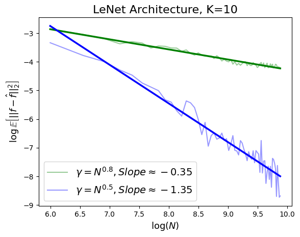
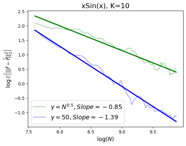
Figure 1: Log-log plot illustrating the convergence rates of approximation error for the function $f(x)=x\sin(x)$ and LeNet5 network under various number of adversarial worker nodes.

V Experimental Results

In this section, we evaluate the performance of the proposed scheme in different adversarial settings. Two types of computing functions are considered: a one-dimensional function $f_{1}(x)=x\sin(x)$ and the LeNet5 neural network [26], a high-dimensional function $\mathbf{f}_{2}:\mathbb{R}^{1024}\to\mathbb{R}^{10}$ trained for handwritten image classification. Equidistant points are used for both the encoder and decoder. The scheme’s approximation error is quantified as empirical approximation of $\mathrm{E}_{\mathbf{x}\sim\mathcal{X}}[\mathcal{R}(\hat{\mathbf{f}})]$, averaged over 20 repetitions for each $N$.

The adversary’s strategy is defined as modifying the values of $f(u_{\textrm{e}}(\beta_{i}))$ for all $\beta_{i}$ near $\{\alpha_{k}\}_{k=1}^{K}$. Specifically, the adversary changes $\frac{\gamma}{K}$ values around each $\alpha_{i}$ for $i\in[K]$ to maximum acceptable value $M$. As shown in Figure 1, for $\gamma=N^{0.8}$, the average approximation error for LeNet5 network converges at a rate of $N^{-0.35}$, which is smaller than the theoretical upper bound of $N^{-0.24}$ given by Corollary 1. Similarly, for $\gamma=N^{0.5}$, the approximation error converges at rates of $N^{-0.85}$ for $f_{1}(x)$ and $N^{-1.35}$ for the LeNet5 network, both smaller than the theoretical upper bound of $N^{-0.6}$. Additionally, a rate of $N^{-1.39}$ is achieved with $\gamma=50$ and $f_{1}(x)$, with a theoretical upper bound of $N^{-1.2}$.

VI Proof Sketch

In this section, we provide a proof sketch for the main theorems. The formal proof can be found in Appendix. To prove Theorem 1, we show that for the function $f(x)=x$, and the case $\gamma=\mu N$ for some $\mu\in(0,1)$, there is no encoder and decoder functions that $\lim_{N\to\infty}\mathcal{R}(\hat{f})=0$. In this case, $f(u_{\textrm{e}}(x))=u_{\textrm{e}}(x)$, which is a spline function defined on the set $\{\alpha_{k}\}_{k=1}^{K}$. First, note that if $\lim_{N\to\infty}\lambda_{\textrm{d}}\neq 0$, the proof becomes trivial, as the decoder function converges to a second-degree polynomial as $N$ increases, while the encoder function remains a piecewise degree-3 polynomial. Therefore, we assume that $\lim_{N\to\infty}\lambda_{\textrm{d}}=0$. Let $\alpha_{\min}=\max(0,\alpha-\frac{\gamma}{2})$ and $\alpha_{\max}=\min(1,\alpha+\frac{\gamma}{2})$. Assume that $u_{\textrm{e}}(\alpha_{\lfloor\frac{K}{2}\rfloor})-x_{\lfloor\frac{K}{2}\rfloor}=\delta$. Define $y_{a}=u_{\textrm{e}}(\alpha_{\lfloor\frac{K}{2}\rfloor})+\Delta+2|\delta|$. Consider the set $\mathcal{V}=\{i:\beta_{i}\in[\alpha_{\text{min}},\alpha_{\text{max}}]\}$. It can be verified that $|\mathcal{V}|\leq\mu$.

Let $P(\cdot)$ be a degree-7 polynomial that satisfies $P^{(j)}(\alpha_{\text{min}})=u_{\textrm{e}}^{(j)}(\alpha_{\text{min}})$, $P^{(j)}(\alpha_{\text{max}})=u_{\textrm{e}}^{(j)}(\alpha_{\text{max}})$, for $j\leqslant 2$, and $P(\alpha_{\lfloor\frac{K}{2}\rfloor})=y_{a}$. With seven degrees of freedom in $P(\cdot)$ and these seven constraints, the adversary can configure $P(\cdot)$ to satisfy all conditions. The adversary then changes the computed value of worker node $i\in\mathcal{V}$ from $f(u_{\textrm{e}}(\beta_{i}))$ to $P(\beta_{i})$. As a result, the master node receives $\overline{\mathbf{y}}_{i}=f(u_{\textrm{e}}(\beta_{i})$, for $\beta_{i}\notin[\alpha_{\text{min}},\alpha_{\text{max}}]$, and $P(\beta_{i})$, otherwise, from the worker nodes.

Consider the following function

$$\widetilde{f}(x)=\begin{cases}f(u_{\textrm{e}}(x))&\text{if }x\notin[\alpha_{\text{min}},\alpha_{\text{max}}],\\ P(x)&\text{if }x\in[\alpha_{\text{min}},\alpha_{\text{max}}].\end{cases}$$ (7)

It can be verified that $\widetilde{f}(\cdot)$ has bounded first and second derivatives, and thus $\widetilde{f}(\cdot)\in\mathcal{H}^{2}\left(\Omega\right)$. Using the error bound for smoothing splines in Sobolev space functions (see Lemma 1), we have:

$$|u_{\textrm{d}}(\alpha_{\lfloor\frac{K}{2}\rfloor})-\widetilde{f}(\alpha_{\lfloor\frac{K}{2}\rfloor})|\leqslant\sup_{z}|u_{\textrm{d}}(z)-\widetilde{f}(z)|\leqslant\mathcal{O}(\lambda_{\textrm{d}}^{\frac{3}{4}}+N^{-3}).$$

Since $\lambda_{\textrm{d}}>C_{\lambda}N^{-4}$ and $\lim_{N\to\infty}\lambda_{\textrm{d}}=0$, for every $|\delta|>\epsilon>0$, there exists $n_{0}\in\mathbb{N}$ such that for $N>n_{0}$, $|u_{\textrm{d}}(\alpha_{\lfloor\frac{K}{2}\rfloor})-\widetilde{f}(\alpha_{\lfloor\frac{K}{2}\rfloor})|\leqslant\epsilon<|\delta|.$ Thus, we have:

$$u_{\textrm{d}}(\alpha_{\lfloor\frac{K}{2}\rfloor})-x_{\lfloor\frac{K}{2}\rfloor}=u_{\textrm{d}}(\alpha_{\lfloor\frac{K}{2}\rfloor})-u_{\textrm{e}}(\alpha_{\lfloor\frac{K}{2}\rfloor})+\delta=u_{\textrm{d}}(\alpha_{\lfloor\frac{K}{2}\rfloor})-\widetilde{f}(\alpha_{\lfloor\frac{K}{2}\rfloor})+\Delta+2|\delta|+\delta\geqslant\Delta+|\delta|+\delta\geqslant\Delta.$$

To prove Theorem 2, note that since $|f^{\prime}|\leqslant\nu$, for some $\nu\in\mathbb{R}_{+}$, function $f$ is $\nu$-Lipschitz. Thus:

$$\mathcal{L}_{\textrm{enc}} =\frac{2}{K}\sum^{K}_{k=1}\left(f(u_{\textrm{e}}(\alpha_{k}))-f(x_{k})\right)^{2}\leqslant\frac{2\nu^{2}}{K}\sum^{K}_{k=1}(u_{\textrm{e}}(\alpha_{k})-x_{k})^{2}.$$ (8)

Let $u_{\textrm{d}}^{\circ}(\cdot)$ represent the decoder function if all server nodes were honest, i.e., $\bar{y}_{n}=f(u_{\textrm{e}}(\beta_{n}))$, for all $n\in[N]$. Thus, from (3), we have:

$$u_{\textrm{d}}^{\circ}=\underset{u\in\mathcal{H}^{2}\left(\Omega\right)}{\operatorname{argmin}}\frac{1}{N}\sum^{N}_{n=1}\left(u\left(\beta_{n}\right)-f(u_{\textrm{e}}(\beta_{n}))\right)^{2}+\lambda_{\textrm{d}}\int_{\Omega}u^{\prime\prime}(t)^{2}\,dt.$$ (9)

Then, starting from $\mathcal{L}_{\textrm{dec}}$ in (III), we have:

$$\mathcal{L}_{\textrm{dec}}(\hat{f}) \stackrel{{\scriptstyle\text{}}}{{=}} \mathop{\sup}_{\mathcal{A}_{\gamma}}\frac{2}{K}\sum^{K}_{k=1}\left|u_{\textrm{d}}\left(\alpha_{k}\right)-f\left(u_{\textrm{e}}\left(\alpha_{k}\right)\right)\right|^{2}$$

$$\stackrel{{\scriptstyle\text{}}}{{\leqslant}}2 \mathop{\sup}_{\mathcal{A}_{\gamma}}\mathop{\sup}_{z}\left|u_{\textrm{d}}\left(z\right)-f\left(u_{\textrm{e}}\left(z\right)\right)\right|^{2}$$

$$\stackrel{{\scriptstyle\text{}}}{{=}}2 \mathop{\sup}_{\mathcal{A}_{\gamma}}\mathop{\sup}_{z}\left|u_{\textrm{d}}\left(z\right)-u_{\textrm{d}}^{\circ}\left(z\right)+u_{\textrm{d}}^{\circ}\left(z\right)-f\left(u_{\textrm{e}}\left(z\right)\right)\right|^{2}$$

$$\stackrel{{\scriptstyle\text{(a)}}}{{\leqslant}} \underbrace{4\mathop{\sup}_{\mathcal{A}_{\gamma}}\mathop{\sup}_{z}|u_{\textrm{d}}\left(z\right)-u_{\textrm{d}}^{\circ}\left(z\right)|^{2}}_{\mathcal{L}_{\textrm{dec}}^{a}(\hat{f})}+\underbrace{4\mathop{\sup}_{z}|u_{\textrm{d}}^{\circ}\left(z\right)-f\left(u_{\textrm{e}}\left(z\right)\right)|^{2}}_{\mathcal{L}_{\textrm{dec}}^{g}(\hat{f})},$$ (10)

where (a) follows by the AM-GM inequality. Note that, $\mathcal{L}_{\textrm{dec}}^{g}(\hat{f})$ in (VI) represents the maximum decoder error in the non-adversarial regime. Thus, it represents a special case of [6], where there is no stragglers. By defining $h(t):=u_{\textrm{d}}^{\circ}(t)-f(u_{\textrm{e}}(t))$ and leveraging the results in [6], we can prove the following lemma:

Lemma 1.

Consider the proposed scheme with the same assumptions as in Theorem 2. Then, we have $\mathcal{L}_{\textrm{dec}}^{g}(\hat{f})=4\left\lVert h\right\rVert^{2}_{{L}^{\infty}\left(\Omega\right)}\leqslant 4\left\lVert(f\circ u_{\textrm{e}})^{(2)}\right\rVert^{2}_{{L}^{2}\left(\Omega\right)}\left(c_{4}\lambda_{\textrm{d}}^{\frac{3}{4}}+c_{5}N^{-3}\right)$, where $c_{4},c_{5}$ are constants.

To complete the proof of Theorem 2, we also need to develop an upper bound for $\mathcal{L}_{\textrm{dec}}^{a}(\hat{f})$ in (VI). To do so, in [23] it is shown that solution of the optimization (9) is a linear operator and can be expressed as follows:

$$u_{\textrm{d}}^{\circ}(x)=\frac{1}{N}\sum_{i=1}^{N}G_{N,\lambda_{\textrm{d}}}(x,\beta_{i})y_{i},$$

where, $y_{i}:=f(u_{\textrm{e}}(\beta_{i}))$ for $i\in[N]$. The weight function $G_{N,\lambda_{\textrm{d}}}(\cdot)$ has a complex dependence on the points $\{\beta_{i}\}_{i=1}^{N}$ and the smoothing parameter $\lambda_{\textrm{d}}$. Consequently, obtaining an explicit expression for it, is quite challenging [27, 28]. However, in [28, 29, 30] $G_{N,\lambda_{\textrm{d}}}(x,t)$ is approximated by a well-defined kernel function $K_{\lambda_{\textrm{d}}}(x,t)$ for the case where $\{\beta_{i}\}^{N}_{i=1}$ are equidistant. Thus, we have:

$$u_{\textrm{d}}(x)\approx\frac{1}{N}\sum_{i=1}^{N}K_{\lambda_{\textrm{d}}}(x,\beta_{i})\overline{y}_{i},\quad u_{\textrm{d}}^{\circ}(x)\approx\frac{1}{N}\sum_{i=1}^{N}K_{\lambda_{\textrm{d}}}(x,\beta_{i})y_{i}.$$

Here, the kernel function $K_{\lambda_{\textrm{d}}}(x,\beta)$ has a bandwidth of $\mathcal{O}(\lambda_{\textrm{d}}^{\frac{1}{4}})$ and its absolute value is bounded by $\tau\lambda_{\textrm{d}}^{\frac{1}{4}}\exp(|x-\beta|\lambda_{\textrm{d}}^{-\frac{1}{4}})$, for some constant $\tau>0$ [29, 28].

Using the properties of the $K_{\lambda_{\textrm{d}}}(\cdot,\cdot)$ outlined in [29, 28], it can be shown that if $\{\beta_{i}\}_{i=1}^{N}$ are equidistant and $N\lambda_{\textrm{d}}^{\frac{1}{4}}>c_{0}$ for some constant $c_{0}>0$, then there exist positive constants $c_{3}$ and $c_{4}$ depending on $c_{0}$, such that:

$$\sup_{0\leq x,\beta\leq 1}\left|G_{N,\lambda_{\textrm{d}}}(x,\beta)-K_{\lambda_{\textrm{d}}}(x,\beta)\right|<\frac{c_{3}}{N}+c_{4}\lambda_{\textrm{d}}^{-\frac{1}{4}}\exp({-\frac{1}{\sqrt{2}}\lambda_{\textrm{d}}^{-\frac{1}{4}}}).$$

Using the kernel representation of $u_{\textrm{d}}(\cdot),u_{\textrm{d}}^{\circ}(\cdot)$, we have:

$$|u_{\textrm{d}}\left(z\right)-u_{\textrm{d}}^{\circ}(z)| \stackrel{{\scriptstyle\text{}}}{{=}}|\frac{1}{N}\sum_{i=1}^{N}G_{N,\lambda}(z,\beta_{i})(\overline{y}_{i}-y_{i})|$$

$$\stackrel{{\scriptstyle\text{}}}{{=}}\left|\frac{1}{N}\sum_{i=1}^{N}\left(G_{N,\lambda}(z,\beta_{i})-K_{\lambda}(z,\beta_{i})\right)\overline{y}_{i}+\frac{1}{N}\sum_{i=1}^{N}K_{\lambda}(z,\beta_{i})(\overline{y}_{i}-y_{i})+\frac{1}{N}\sum_{i=1}^{N}\left(K_{\lambda}(z,\beta_{i})-G_{N,\lambda}(z,\beta_{i})\right){y_{i}}\right|$$

$$\stackrel{{\scriptstyle\text{}}}{{\leqslant}}\frac{1}{N}\sum_{i=1}^{N}\left|y_{i}-\overline{y}_{i}\right|\left|G_{N,\lambda}(z,\beta_{i})-K_{\lambda}(z,\beta_{i})\right|+\frac{1}{N}\sum_{i=1}^{N}\left|y_{i}-\overline{y}_{i}\right|\left|K_{\lambda}(z,\beta_{i})\right|$$

$$\stackrel{{\scriptstyle\text{}}}{{\leqslant}}\frac{2M\gamma}{N}\sup_{z,\beta\in\{\beta_{i}\}^{N}_{i=1}}\left|G_{N,\lambda}(z,\beta)-K_{\lambda}(z,\beta)\right|+\frac{2M\gamma}{N}\sup_{z,\beta\in\{\beta_{i}\}^{N}_{i=1}}\left|K_{\lambda}(z,\beta)\right|$$

$$\stackrel{{\scriptstyle\text{(a)}}}{{\leqslant}}\frac{2M\gamma}{N}\left(\frac{c_{3}}{N}+c_{4}\lambda_{\textrm{d}}^{-\frac{1}{4}}e^{-\frac{1}{\sqrt{2}}\lambda_{\textrm{d}}^{-\frac{1}{4}}}+\tau\lambda_{\textrm{d}}^{\frac{1}{4}}e^{|x-\beta|\lambda_{\textrm{d}}^{-\frac{1}{4}}}\right),$$

where (a) follows from $\sup_{z,\beta}\left|K_{\lambda}(z,\beta)\right|\leqslant\tau\lambda_{\textrm{d}}^{\frac{1}{4}}\exp(|x-\beta|\lambda_{\textrm{d}}^{-\frac{1}{4}})$. Using the above result with Lemma 1 and (8) completes the proof of Theorem 2.

To prove Theorem 3, we first prove that If $|f^{\prime}|\leqslant\nu$ and $|f^{\prime\prime}|\leqslant\eta$, then there exists a monotonically increasing function $\xi:[0,\infty)\to\mathbb{R}$ such that: $\left\lVert(f\circ u_{\textrm{e}})^{\prime\prime}\right\rVert^{2}_{{L}^{2}\left(\Omega\right)}\leqslant(\eta^{2}+\nu^{2})\cdot\xi\left(\left\lVert u_{\textrm{e}}\right\rVert^{2}_{\widetilde{\mathcal{H}}^{2}\left(\Omega;\mathbb{R}\right)}\right).$ As a result, defining $\psi(t):=2+\xi(t)$ and $\lambda_{\textrm{e}}:=\max\{C_{1}\frac{M^{2}\gamma^{2}}{N^{4}},C_{2}\frac{M^{2}\gamma^{2}}{N^{2}}\lambda_{\textrm{d}}^{-\frac{1}{2}}(e^{({\sqrt{2}}\lambda_{\textrm{d}}^{-\frac{1}{4}})}+C_{3}),(\nu^{2}+\eta^{2})(C_{4}\lambda_{\textrm{d}}^{\frac{3}{4}}+C_{5}N^{-3})\}$ completes the proof of the Theorem 3.

Appendix A Preliminaries: Sobolev spaces and Sobolev norms

Let $\Omega$ be an open interval in $\mathbb{R}$ and $M$ be a positive integer. We denote by ${L}^{p}\left(\Omega;\mathbb{R}^{M}\right)$ the class of all measurable functions $g:\mathbb{R}\to\mathbb{R}^{M}$ that satisfy:

$$\int_{\Omega}|g_{j}(t)|^{p}\,dt\ <\infty,\quad\forall j\in[M],$$ (11)

where $g(\cdot)=[g_{1}(\cdot),\dots,g_{M}(\cdot)]^{T}$. The space ${L}^{p}\left(\Omega;\mathbb{R}^{M}\right)$ can be endowed with the following norm, known as the ${L}^{p}$ norm:

$$\|g\|_{{L}^{p}\left(\Omega;\mathbb{R}^{M}\right)}:=\left(\sum^{M}_{j=1}\int_{\Omega}|g_{i}(t)|^{p}\,dt\right)^{\frac{1}{p}},$$ (12)

for $1\leqslant p<\infty$, and

$$\|g\|_{{L}^{\infty}\left(\Omega;\mathbb{R}^{M}\right)}:=\max_{j\in[M]}\sup_{t\in\Omega}|g_{j}(t)|.$$ (13)

for $p=\infty$. Additionally, a function $g:\Omega\to\mathbb{R}^{M}$ is in ${L}_{\textrm{loc}}^{p}\left(\Omega;\mathbb{R}^{M}\right)$ if it lies in ${L}^{p}(V;\mathbb{R}^{M})$ for all compact subsets $V\subseteq\Omega$.

Definition 1 (Sobolev Space).

The Sobolev space $\mathbb{W}^{m,p}\left(\Omega;\mathbb{R}^{M}\right)$ is the space of all functions $g\in{L}^{p}\left(\Omega;\mathbb{R}^{M}\right)$ such that all weak derivatives of order $i$, denoted by $g^{(i)}$, belong to ${L}^{p}\left(\Omega;\mathbb{R}^{M}\right)$ for $i\in[m]$. This space is endowed with the norm:

$$\left\lVert g\right\rVert_{\mathbb{W}^{m,p}\left(\Omega;\mathbb{R}^{M}\right)}:=\left(\left\lVert g\right\rVert_{{L}^{p}\left(\Omega;\mathbb{R}^{M}\right)}^{p}+\sum^{m}_{i=1}\left\lVert g^{(i)}\right\rVert_{{L}^{p}\left(\Omega;\mathbb{R}^{M}\right)}^{p}\right)^{\frac{1}{p}},$$ (14)

for $1\leqslant p<\infty$, and

$$\|g\|_{\mathbb{W}^{m,\infty}\left(\Omega;\mathbb{R}^{M}\right)}:=\max\left\{\left\lVert g\right\rVert_{{L}^{\infty}\left(\Omega;\mathbb{R}^{M}\right)},\max_{i\in[m]}\left\lVert g^{(i)}\right\rVert_{{L}^{\infty}\left(\Omega;\mathbb{R}^{M}\right)}\right\},$$ (15)

for $p=\infty$.

Similarly, $\mathbb{W}_{\textrm{loc}}^{m,p}\left(\Omega;\mathbb{R}^{M}\right)$ is defined as the space of all functions $g\in{L}_{\textrm{loc}}^{p}\left(\Omega;\mathbb{R}^{M}\right)$ with all weak derivatives of order $i$ belonging to ${L}_{\textrm{loc}}^{p}\left(\Omega;\mathbb{R}^{M}\right)$ for $i\in[m]$. $\left\lVert g\right\rVert_{\mathbb{W}_{\textrm{loc}}^{m,p}\left(\Omega;\mathbb{R}^{M}\right)}$ and $\left\lVert g\right\rVert_{\mathbb{W}_{\textrm{loc}}^{m,\infty}\left(\Omega;\mathbb{R}^{M}\right)}$ are defined similar to (14) and (17) respectively, using ${L}_{\textrm{loc}}^{p}\left(\Omega;\mathbb{R}\right)$ instead of ${L}^{p}\left(\Omega\right)$.

Definition 2.

(Sobolev Space with compact support): Denoted by $\mathbb{W}_{0}^{m,p}\left(\Omega;\mathbb{R}^{M}\right)$ collection of functions $g$ defined on interval $\Omega=(a,b)$ such that $g(a)=\mathbf{0},g^{\prime}(a)=\mathbf{0},\dots,g^{(m-1)}(a)=\mathbf{0}$ and $\left\lVert g^{(m)}\right\rVert_{{L}^{2}\left(\Omega\right)}<\infty$. This space can be endowed with the following norm:

$$\left\lVert g\right\rVert_{\mathbb{W}^{m,p}\left(\Omega;\mathbb{R}^{M}\right)}:=\left\lVert g^{(m)}\right\rVert_{{L}^{p}\left(\Omega;\mathbb{R}^{M}\right)},$$ (16)

for $1\leqslant p<\infty$, and

$$\|g\|_{\mathbb{W}^{m,\infty}\left(\Omega;\mathbb{R}^{M}\right)}:=\left\lVert g^{(m)}\right\rVert_{{L}^{\infty}\left(\Omega;\mathbb{R}^{M}\right)},$$ (17)

for $p=\infty$.

The next theorem provides an upper bound for ${L}^{p}$ norm of functions in the Sobolev space, which plays a crucial role in the proof of the main theorems of the paper.

Theorem 5 (Theorem 7.34, [31]).

Let $\Omega\subseteq\mathbb{R}$ be an open interval and let $g\in\mathbb{W}_{\textrm{loc}}^{1,1}\left(\Omega;\mathbb{R}^{M}\right)$. Assume $1\leqslant p,q,r\leqslant\infty$ and $r\geqslant q$. Then:

$$\left\lVert g\right\rVert_{{L}^{r}\left(\Omega;\mathbb{R}^{M}\right)}\leqslant\ell^{\frac{1}{r}-\frac{1}{q}}\left\lVert g\right\rVert_{{L}^{q}\left(\Omega;\mathbb{R}^{M}\right)}+\ell^{1-\frac{1}{p}+\frac{1}{r}}\left\lVert g^{\prime}\right\rVert_{{L}^{p}\left(\Omega;\mathbb{R}^{M}\right)},$$ (18)

for every $0<\ell<\mathcal{L}^{1}(\Omega)$.

Note that $\mathcal{L}^{1}(\Omega)$ in Theorem 5 is the length of the interval $\Omega$.

Corollary 2.

Suppose $g\in\mathbb{W}_{\textrm{loc}}^{1,1}\left(\Omega;\mathbb{R}^{M}\right)$ and $\Omega\subseteq\mathbb{R}$ be an open interval. If $\frac{\left\lVert g\right\rVert_{{L}^{2}\left(\Omega;\mathbb{R}^{M}\right)}}{\left\lVert g^{\prime}\right\rVert_{{L}^{2}\left(\Omega;\mathbb{R}^{M}\right)}}<\mathcal{L}^{1}(\Omega)$, then:

$$\left\lVert g\right\rVert_{{L}^{\infty}\left(\Omega;\mathbb{R}^{M}\right)}\leqslant 2\sqrt{\left\lVert g\right\rVert_{{L}^{2}\left(\Omega;\mathbb{R}^{M}\right)}\cdot\left\lVert g^{\prime}\right\rVert_{{L}^{2}\left(\Omega;\mathbb{R}^{M}\right)}}.$$ (19)

Proof.

Substituting $p,q=2$ and $r=\infty$ in Theorem 5 and optimizing over $\ell$, one can derive the optimum value of $\ell$, denoted by $\ell^{*}$ as

$$\ell^{*}=\frac{\left\lVert g\right\rVert_{{L}^{2}\left(\Omega;\mathbb{R}^{M}\right)}}{\left\lVert g^{\prime}\right\rVert_{{L}^{2}\left(\Omega;\mathbb{R}^{M}\right)}}.$$ (20)

Since $\frac{\left\lVert g\right\rVert_{{L}^{2}\left(\Omega;\mathbb{R}^{M}\right)}}{\left\lVert g^{\prime}\right\rVert_{{L}^{2}\left(\Omega;\mathbb{R}^{M}\right)}}<\mathcal{L}^{1}(\Omega)$, the optimum value is in the valid interval mentioned in Theorem 5. ∎

Corollary 3 (Corollary 7.36, [31]).

Let $\Omega=(a,b)$, let $1\leq p,q,r\leq\infty$ be such that $1+1/r\geq$ $1/p$ and $r\geq q$ and let $g\in\mathbb{W}_{\textrm{loc}}^{1,1}\left(\Omega;\mathbb{R}^{M}\right)$ with $g^{\prime}\in{L}^{p}\left(\Omega;\mathbb{R}^{M}\right)$. Let $x_{0}\in[a,b]$ be such that $\left|g\left(x_{0}\right)\right|=\min_{[a,b]}|g|$. Then

$$\left\|g-g\left(x_{0}\right)\right\|_{{L}^{r}\left(\Omega;\mathbb{R}^{M}\right)}\leq 8\|g\|_{{L}^{q}\left(\Omega;\mathbb{R}^{M}\right)}^{\alpha}\left\|g^{\prime}\right\|_{{L}^{p}\left(\Omega;\mathbb{R}^{M}\right)}^{1-\alpha}$$ (21)

where $\alpha:=0$ if $r=q$ and $1-1/p+1/r=0$ and otherwise

$$\alpha:=\frac{1-1/p+1/r}{1-1/p+1/q}.$$

Corollary 4.

[6, Corollary 3] Theorem 5 and Corollary 3 hold true when $f\in\mathbb{W}^{2,2}\left(\Omega;\mathbb{R}^{M}\right)$.

Equivalent norms. There have been various norms defined on Sobolev spaces in the literature that are equivalent to (14) (see [32], [33, Ch. 7], and [24, Sec. 10.2]). Note that two norms $\left\lVert\cdot\right\rVert_{W_{1}},\left\lVert\cdot\right\rVert_{W_{2}}$ are equivalent if there exist positive constants $\eta_{1},\eta_{2}$ such that $\eta_{1}\cdot\left\lVert g\right\rVert_{W_{2}}\leqslant\left\lVert g\right\rVert_{W_{1}}\leqslant\eta_{2}\cdot\left\lVert g\right\rVert_{W_{2}}$. The equivalent norm in which we are interested is the one introduced in [34]. Let $\Omega=(a,b)\subset\mathbb{R}$. We define $\widetilde{\mathbb{W}}^{m,p}\left(\Omega;\mathbb{R}^{M}\right)$ as the Sobolev space endowed with the following norm:

$$\left\lVert g\right\rVert_{\widetilde{\mathbb{W}}^{m,p}\left(\Omega;\mathbb{R}^{M}\right)}:=\left(\sum^{M}_{j=1}\left(g_{j}(a)^{p}+\sum^{m-1}_{i=1}\left(g_{j}^{(i)}(a)\right)^{p}\right)+\left\lVert g^{(m)}\right\rVert_{{L}^{p}\left(\Omega;\mathbb{R}^{M}\right)}^{p}\right)^{\frac{1}{p}}.$$ (22)

The following lemma derives the equivalence constants ($\eta_{1},\eta_{2}$) for the norms $\left\lVert\cdot\right\rVert_{\mathbb{W}^{2,2}\left(\Omega;\mathbb{R}\right)}$ and $\left\lVert\cdot\right\rVert_{\widetilde{\mathbb{W}}^{2,2}\left(\Omega;\mathbb{R}\right)}$.

Lemma 2.

[6, Lemma 1] Let $\Omega=(a,b)$ be an arbitrary open interval in $\mathbb{R}$. Then for every $g\in\mathbb{W}^{2,2}\left(\Omega;\mathbb{R}\right)$:

$$\left\lVert g\right\rVert^{2}_{\mathbb{W}^{2,2}\left(\Omega;\mathbb{R}\right)}\leqslant\left[2(b-a)\max\{1,(b-a)\}\left(2\max\{1,(b-a)\}^{2}+1\right)+1\right]\cdot\left\lVert g\right\rVert^{2}_{\widetilde{\mathbb{W}}^{2,2}\left(\Omega;\mathbb{R}\right)}$$ (23)

$$\left\lVert g\right\rVert^{2}_{\widetilde{\mathbb{W}}^{2,2}\left(\Omega;\mathbb{R}\right)}\leqslant\left(\frac{4}{(b-a)}\max\{1,(b-a)\}^{2}+1\right)\cdot\left\lVert g\right\rVert^{2}_{\mathbb{W}^{2,2}\left(\Omega;\mathbb{R}\right)}.$$ (24)

Corollary 5.

Based on Lemma 2, for $\Omega=(0,1)$ we have

$$\frac{1}{5}\cdot\left\lVert g\right\rVert^{2}_{\widetilde{\mathbb{W}}^{2,2}\left(\Omega;\mathbb{R}\right)}\leqslant\left\lVert g\right\rVert^{2}_{\mathbb{W}^{2,2}\left(\Omega;\mathbb{R}\right)}\leqslant 7\cdot\left\lVert g\right\rVert^{2}_{\widetilde{\mathbb{W}}^{2,2}\left(\Omega;\mathbb{R}\right)}.$$ (25)

Corollary 5 directly follows from Lemma 2 by substituting $(a,b)=(0,1)$.

Corollary 6.

The result of Lemma 2 remains valid for multi-dimensional cases, where $g:\mathbb{R}\to\mathbb{R}^{M}$, for $M>1$.

Corollary 6 directly follows from applying Lemma 2 to each component of the function $g(\cdot)$ and using the definition of vector-valued function norm:

$$\left\lVert g\right\rVert^{2}_{\mathbb{W}^{2,2}\left(\Omega;\mathbb{R}^{M}\right)}=\sum^{M}_{j=1}\left\lVert g^{(j)}\right\rVert^{2}_{\mathbb{W}^{2,2}\left(\Omega;\mathbb{R}\right)},\quad\left\lVert g\right\rVert^{2}_{\widetilde{\mathbb{W}}^{2,2}\left(\Omega;\mathbb{R}^{M}\right)}=\sum^{M}_{j=1}\left\lVert g^{(j)}\right\rVert^{2}_{\widetilde{\mathbb{W}}^{2,2}\left(\Omega;\mathbb{R}\right)}.$$

Proposition 1.

([31, Section 7.2], [33, Theorem 121],[24]) For any open interval $\Omega\subseteq\mathbb{R}$ and $m,M\in\mathbb{N}$,

$$\mathcal{H}^{m}_{M}\left(\Omega\right) :=\mathbb{W}^{m,2}\left(\Omega;\mathbb{R}^{M}\right),$$

$$\widetilde{\mathcal{H}}^{m}\left(\Omega;\mathbb{R}^{M}\right) :=\widetilde{\mathbb{W}}^{m,2}\left(\Omega;\mathbb{R}^{M}\right),$$

$$\mathcal{H}_{0}^{m}\left(\Omega;\mathbb{R}^{M}\right) :=\mathbb{W}_{0}^{m,2}\left(\Omega;\mathbb{R}^{M}\right),$$ (26)

are Reproducing Kernel Hilbert Spaces (RKHSs).

The full expression of the kernel function of $\mathcal{H}^{m}\left(\Omega\right)$ and $\widetilde{\mathcal{H}}^{m}\left(\Omega;\mathbb{R}\right)$ and other equivalent norms of Sobolev spaces can be found in [33, Section 4]. For $\widetilde{\mathcal{H}}^{m}\left(\Omega;\mathbb{R}\right)$ the kernel function is as follows:

$$R(t,s)=\sum_{j=0}^{m-1}\frac{t^{j}s^{j}}{j!^{2}}+\int_{\Omega}\frac{(t-x)_{+}^{m-1}(s-x)_{+}^{m-1}}{(m-1)!^{2}}\,dx,$$ (27)

where $(\cdot)_{+}$ is positive part function.

Appendix B Smoothing Splines

Consider the data model $y_{i}=f(t_{i})+\epsilon_{i}$ for $i=1,\dots,n$, where $t_{i}\in\Omega=(a,b)\subset\mathbb{R}$, $\mathbb{E}[\epsilon_{i}]=0$, and $\mathbb{E}[\epsilon_{i}^{2}]\leqslant\sigma_{0}^{2}$. Assuming $f\in\widetilde{\mathbb{W}}^{m,2}\left(\Omega;\mathbb{R}\right)$, the solution to the following optimization problem is referred to as the smoothing spline:

$$\mathbf{S}_{\lambda,n,m}[\mathbf{y}]:=\underset{g\in\widetilde{\mathbb{W}}^{m,2}\left(\Omega;\mathbb{R}\right)}{\operatorname{argmin}}\frac{1}{n}\sum^{n}_{i=1}\left(g\left(t_{i}\right)-y_{i}\right)^{2}+\lambda\int_{\Omega}\left(g^{(m)}(t)\right)^{2}\,dt,$$ (28)

where $\mathbf{y}=[y_{1},\dots,y_{n}]$. Based on Proposition 1, $\widetilde{\mathcal{H}}^{m}\left(\Omega;\mathbb{R}\right):=\widetilde{\mathbb{W}}^{m,2}\left(\Omega;\mathbb{R}\right)$ with the norm $\left\lVert\cdot\right\rVert_{\widetilde{\mathbb{W}}^{m,2}\left(\Omega;\mathbb{R}\right)}$ is a RKHS for some kernel function $\phi(\cdot,\cdot)$. Therefore for any $v\in\widetilde{\mathbb{W}}^{m,2}\left(\Omega;\mathbb{R}\right)$, we have:

$$v(t)=\langle v(\cdot),\phi(\cdot,t)\rangle_{\widetilde{\mathcal{H}}^{m}\left(\Omega;\mathbb{R}\right)}.$$ (29)

It can be shown that $\phi(t,s)=R^{P}(t,s)+\phi_{0}(t,s)$ where $\phi_{0}(t,s)$ is kernel function of $\mathcal{H}_{0}^{m}\left(\Omega\right)$ and $R^{P}(t,s)$ is a null space of $\mathcal{H}_{0}^{m}\left(\Omega\right)$ which is the space of all polynomials with degree less than $m$.

The solution of (28) has the following form [24, 35]:

$$u^{*}(\cdot)=\sum^{m}_{i=1}d_{i}\zeta_{i}(\cdot)+\sum^{n}_{j=1}c_{j}\phi_{0}(\cdot,t_{j}),$$ (30)

where $\left\{\zeta_{i}(\cdot)\right\}_{i=1}^{m}$ are the basis functions of the space of polynomials of degree at most $m-1$. Substituting $u^{*}$ into (28) and optimizing over $\mathbf{c}=[c_{1},\dots,c_{n}]^{T}$ and $\mathbf{d}=[d_{1},\dots,d_{m}]^{T}$, we obtain the following result [24]:

$$\mathbf{S}_{\lambda,n,m}[\mathbf{y}](\mathbf{y}) =\mathbf{Q}\left(\mathbf{Q}^{T}\mathbf{Q}+\lambda\mathbf{\Gamma}\right)^{-1}\mathbf{Q}^{T}\mathbf{y},$$ (31)

$$\mathbf{d} =\left(\mathbf{P}^{T}\mathbf{L}^{-1}\mathbf{P}\right)^{-1}\mathbf{P}^{T}\mathbf{L}^{-1}\mathbf{y},$$ (32)

$$\mathbf{c} =\mathbf{L}^{-1}\left(\mathbf{I}-\mathbf{P}\left(\mathbf{P}^{T}\mathbf{L}^{-1}\mathbf{P}\right)^{-1}\mathbf{P}^{T}\mathbf{L}^{-1}\right)\mathbf{y},$$ (33)

where

$$\mathbf{Q}_{n\times(n+m)} =\left[\begin{array}[]{ll}\mathbf{P}_{n\times m}&\bm{\Sigma}_{n\times n}\end{array}\right],$$ (35)

$$\mathbf{\Gamma}_{(n+m)\times(n+m)} =\left[\begin{array}[]{cc}\mathbf{0}_{m\times m}&\mathbf{0}_{m\times n}\\ \mathbf{0}_{n\times 1}&\bm{\Sigma}_{n\times n}\end{array}\right],$$ (37)

$$\bm{P}_{ij} =\zeta_{j}(t_{i}),$$

$$\bm{\Sigma}_{ij} =\phi_{0}(t_{i},t_{j}),$$

$$\mathbf{L} =\mathbf{\Sigma}+n\lambda\mathbf{I}.$$ (38)

Equation (31) states that the smoothing spline fitted on the data points $\mathbf{y}$ is a linear operator:

$$\mathbf{S}_{\lambda,n,m}[\mathbf{y}](\mathbf{z}):=\mathbf{A_{\lambda}}\mathbf{z},$$ (39)

for $\mathbf{z}\in\mathbb{R}^{n}$, where $\mathbf{A_{\lambda}}:=\mathbf{Q}\left(\mathbf{Q}^{T}\mathbf{Q}+\lambda\mathbf{\Gamma}\right)^{-1}\mathbf{Q}^{T}$.

To characterize the estimation error of the smoothing spline, $|f-\mathbf{S}_{\lambda,n,m}(\mathbf{y})|$, we need to define two variables quantify the minimum and maximum consecutive distance of the regression points $\{t_{i}\}^{n}_{i=1}$:

$$\Delta_{\textrm{max}}:=\underset{i\in\{0\}\cup[n]}{\max}\left\{t_{i+1}-t_{i}\right\},\quad\Delta_{\textrm{min}}:=\underset{i\in[n-1]}{\min}\left\{t_{i+1}-t_{i}\right\},$$ (40)

where boundary points are defined as $(t_{0},t_{n+1}):=(a,b)$. The following theorem offers an upper bound for the $j$-th derivative of the smoothing spline estimator error function in the absence of noise ($\sigma_{0}=0$).

Theorem 6.

([36, Theorem 4.10]) Consider data model $y_{i}=f(t_{i})$ with $\{t_{i}\}^{n}_{i=1}$ belong to $\Omega=[a,b]$ for $i\in[n]$. Let

$$L=p_{2(m-1)}(\frac{\Delta_{\textrm{max}}}{\Delta_{\textrm{min}}})\cdot\frac{n\Delta_{\textrm{max}}}{b-a}\frac{\lambda}{2}+D(m)\cdot\left({\Delta_{\textrm{max}}}\right)^{2m},$$ (41)

where $p_{d}(\cdot)$ is a degree $d$ polynomial with positive weights and $D(m)$ is a function of $m$. Then for each $j\in\{0,1,\dots,m\}$ and any $f\in\mathbb{W}^{m,2}\left(\Omega;\mathbb{R}\right)$, there exist a function $H(m,j)$ such that:

$$\left\lVert\left(f-\mathbf{S}_{\lambda,n,m}(\mathbf{y})\right)^{(j)}\right\rVert_{{L}^{2}\left(\Omega\right)}^{2}\leqslant H(m,j)\left(1+\left(\frac{L}{(b-a)^{2m}}\right)\right)^{\frac{j}{m}}\cdot L^{\frac{(m-j)}{m}}\cdot\left\lVert f^{(m)}\right\rVert^{2}_{{L}^{2}\left(\Omega\right)}.$$ (42)

Note that $\left(f-\mathbf{S}_{\lambda,n,m}(\mathbf{y})\right)^{(0)}:=f-\mathbf{S}_{\lambda,n,m}(\mathbf{y})$.

Substituting (33) and (32) into (30), one can conclude that:

$$u^{*}(x)=\bm{\zeta}(x)^{T}\mathbf{M_{1}}\mathbf{y}+\bm{\phi_{0}}(x)^{T}\mathbf{M_{2}}\mathbf{y},$$ (43)

where $\bm{\phi_{0}}(x):=[\phi_{0}(x,t_{1})\dots\phi_{0}(x,t_{n})]^{T}$, $\bm{\zeta}(x):=[\zeta_{1}(x)\dots\zeta_{m}(x)]^{T}$, and matrices $M_{1}$ and $M_{2}$ are defined as $\mathbf{M_{1}}:=\left(\mathbf{P}^{T}\mathbf{L}^{-1}\mathbf{P}\right)^{-1}\mathbf{P}^{T}\mathbf{L}^{-1}$ and $\mathbf{M_{2}}\,:=\,\mathbf{L}^{-1}\left(\mathbf{I}-\mathbf{P}\left(\mathbf{P}^{T}\mathbf{L}^{-1}\mathbf{P}\right)^{-1}\mathbf{P}^{T}\mathbf{L}^{-1}\right)$. Thus, there exists a weight function, denoted by $G_{n,\lambda}(x,t)$, such that:

$$u^{*}(x)=\frac{1}{n}\sum_{i=1}^{n}G_{n,\lambda}(x,t_{i})y_{i},$$ (44)

where $G_{n,\lambda}(x,t)$ depends on the regression points $\{t_{i}\}_{i=1}^{n}$ and the smoothing parameter $\lambda$.

Obtaining an explicit expression for $G_{n,\lambda}(x,t)$ is challenging due to the complexity of the inverse matrix operation and the kernel of $\mathcal{H}^{2}_{1}\left(\Omega\right)$ in general cases. However, it has been shown that the weight function $G_{n,\lambda}(x,t)$ can be approximated by a well-defined kernel function $K_{\lambda}(x,t)$ under certain assumptions about the regression points ${t_{i}}_{i=1}^{n}$ [27, 28, 29, 30].

In an early work, [27] proposed the following kernel function:

$$\kappa(u)=\frac{1}{2}\exp\left(\frac{-|u|}{\sqrt{2}}\right)\sin\left(\frac{|u|}{\sqrt{2}}+\frac{\pi}{4}\right).$$ (45)

[27] demonstrated that for $t$ sufficiently far from the boundary, the following holds:

$$\lambda^{\frac{1}{4}}q(t)^{-\frac{1}{4}}G_{n,\lambda}\left(t+\lambda^{\frac{1}{4}}q(t)^{-\frac{1}{4}}x,t\right)\xrightarrow{n\to\infty}\frac{\kappa(x)}{q(t)},$$ (46)

where $q(t)$ represents the asymptotic probability density function of the regression points.

According to (46), as $n$ increases, the smoothing spline behaves like a kernel smoother with a bandwidth of $\lambda^{\frac{1}{4}}q(t)^{-\frac{1}{4}}$. However, this approximation was later found to be insufficient for establishing certain asymptotic properties [28].

Consider the continuous formulation of the smoothing spline objective over the domain $\Omega=[0,1]$:

$$g^{*}(\cdot):=\underset{g\in\widetilde{\mathbb{W}}^{m,2}\left(\Omega;\mathbb{R}\right)}{\operatorname{argmin}}\int_{0}^{1}\left(f(t)-g(t)\right)^{2},dt+\lambda\int_{0}^{1}\left(g^{\prime\prime}(t)\right)^{2},dt.$$ (47)

It can be shown that the solution to (47) is characterized by a unique Green’s function $G_{\lambda}(x,t)$, satisfying:

$$h(x):=\int_{0}^{1}G_{\lambda}(x,t)f(t),dt.$$ (48)

[29] proposed an alternative approximated kernel function for equidistant regression points, i.e. $t_{i}=\frac{i}{n}$, which addresses the asymptotic issues of (46):

$$K_{\lambda}(x,t)= \left(2\sqrt{2}\lambda^{\frac{1}{4}}\right)^{-1}e^{-\frac{|x-t|}{\sqrt{2}\lambda^{\frac{1}{4}}}}\left(\sin\frac{|x-t|}{\sqrt{2}\lambda^{\frac{1}{4}}}+\cos\left(\frac{x-t}{\sqrt{2}\lambda^{\frac{1}{4}}}\right)\right)$$

$$+\left(2\sqrt{2}\lambda^{\frac{1}{4}}\right)^{-1}\left(\Phi\left(\frac{x+t}{\sqrt{2}\lambda^{\frac{1}{4}}},\frac{x-t}{\sqrt{2}\lambda^{\frac{1}{4}}}\right)+\Phi\left(\frac{1-x}{\sqrt{2}\lambda^{\frac{1}{4}}}+\frac{1-t}{\sqrt{2}\lambda^{\frac{1}{4}}},\frac{1-x}{\sqrt{2}\lambda^{\frac{1}{4}}}-\frac{1-t}{\sqrt{2}\lambda^{\frac{1}{4}}}\right)\right),$$ (49)

where, $\Phi(u,v):=e^{-u}\left(\cos(u)-\sin(u)+2\cos(v)\right)$. Note that the absolute values of the kernels in (45) and (B) decay exponentially to zero as the distance $|t-z|$ increases. The bandwidth of the kernels are $\mathcal{O}(\lambda^{\frac{1}{4}})$.

Lemma 3.

For the the kernel function proposed in (B), there exist a constant $\tau$ such that:

$$\sup_{0\leq x,t\leq 1}\left|K_{\lambda}(x,t)\right|\leqslant\tau\lambda^{-\frac{1}{4}}.$$ (50)

Proof.

From (B), and using the bounds $|\sin(x)|\leqslant 1$ and $|\cos(x)|\leqslant 1$, we obtain:

$$K_{\lambda}(x,t) \leqslant\left(\sqrt{2}\lambda^{\frac{1}{4}}\right)^{-1}e^{-\frac{|x-t|}{\sqrt{2}\lambda^{\frac{1}{4}}}}+4\left(\sqrt{2}\lambda^{\frac{1}{4}}\right)^{-1}\left(e^{-\frac{(x+t)}{\sqrt{2}\lambda^{\frac{1}{4}}}}+e^{-\frac{(2-x-t)}{\sqrt{2}\lambda^{\frac{1}{4}}}}\right)\ \leqslant\left(\sqrt{2}\lambda^{\frac{1}{4}}\right)^{-1}+8\left(\sqrt{2}\lambda^{\frac{1}{4}}\right)^{-1}\ \leqslant\frac{9}{\sqrt{2}}\lambda^{-\frac{1}{4}}.$$

∎

The following lemma that characterize the relationship between their proposed kernel $K_{\lambda}(x,t)$ and continuous Green function $G_{\lambda}(x,t)$:

Lemma 4.

[29, Theorem 4.1] For $0<\lambda\leqslant 1$, there exists constant $C$ such that:

$$\sup_{0\leq x,t\leq 1}\left|K_{\lambda}(x,t)-G_{\lambda}(x,t)\right|\leq C\frac{e^{-\left(\frac{1}{\sqrt{2}}\lambda^{-\frac{1}{4}}\right)}}{\lambda^{\frac{1}{4}}}.$$ (51)

According to Lemma 4, if $\lambda\to 0$ as $n\to\infty$, the proposed kernel converges exponentially to the true Green’s function. Moreover, with an appropriate choice of $\lambda$, in the case of uniform regression points, it can be ensured that the weight function $G_{n,\lambda}(x,t)$ defined in (44) converges to the Green’s function $G_{\lambda}(x,t)$:

Lemma 5.

[30, Theorem 2.1] For uniformly distributed regression points in $[0,1]$, if $n\lambda^{\frac{1}{4}}>C_{0}$ for some constant $C_{0}>0$, then there exist positive constants $\mu_{1}$ and $\mu_{2}$ such that:

$$\sup_{0\leq x,t\leq 1}\left|G_{n,\lambda}(x,t)-\mathrm{G}_{\lambda}(x,t)\right|<\frac{\mu_{1}n^{-1}}{1-\mu_{1}n^{-1}\lambda^{-\frac{1}{4}}}\mathrm{e}^{-{\mu_{2}\left|t-x\right|}{\lambda^{-\frac{1}{4}}}}.$$ (52)

We now present our main lemma, which characterizes the relationship between the weight function $G_{n,\lambda}(x,t)$ and the approximated kernel $K_{\lambda}(x,t)$:

Lemma 6.

For uniformly distributed regression points in $[0,1]$, if $n\lambda^{\frac{1}{4}}>C_{0}$ for some constant $C_{0}>0$ and $0<\lambda\leqslant 1$, then there exist positive constants $\mu_{3}$ and $\mu_{4}$ depending on $C_{0}$, such that:

$$\sup_{0\leq x,t\leq 1}\left|G_{n,\lambda}(x,t)-K_{\lambda}(x,t)\right|<\frac{\mu_{3}}{n}e^{\left(-\lambda^{-\frac{1}{4}}|x-t|\right)}+\mu_{4}\lambda^{-\frac{1}{4}}e^{\left(-\frac{1}{\sqrt{2}}\lambda^{-\frac{1}{4}}\right)}.$$ (53)

Proof.

Lemma 6 can directly derive from Lemma 4 and Lemma 5 and using the fact that:

$$\sup_{0\leq x,t\leq 1}\left|G_{n,\lambda}(x,t)-K_{\lambda}(x,t)\right| \leqslant\sup_{0\leq x,t\leq 1}\left|G_{n,\lambda}(x,t)-G_{\lambda}(x,t)|+|G_{\lambda}(x,t)+K_{\lambda}(x,t)\right|$$

$$\leqslant\sup_{0\leq x,t\leq 1}|G_{n,\lambda}(x,t)-G_{\lambda}(x,t)|+\sup_{0\leq x,t\leq 1}|G_{\lambda}(x,t)+K_{\lambda}(x,t)|$$ (54)

∎

Appendix C Proof of Theorem 2

Recall from (III) and (VI) that $\mathcal{R}(\hat{f})\leqslant\mathcal{L}_{\textrm{enc}}(\hat{f})+\mathcal{L}_{\textrm{dec}}^{a}(\hat{f})+\mathcal{L}_{\textrm{dec}}^{g}(\hat{f})$, where

$$\mathcal{L}_{\textrm{dec}}^{a}(\hat{f}) =4\mathop{\sup}_{\mathcal{A}_{\gamma}}\mathop{\sup}_{z}\left|u_{\textrm{d}}\left(z\right)-u_{\textrm{d}}^{\circ}(z)\right|^{2},$$ (55)

$$\mathcal{L}_{\textrm{dec}}^{g}(\hat{f}) =4\mathop{\sup}_{z}\left|u_{\textrm{d}}^{\circ}\left(z\right)-f(u_{\textrm{e}}(z))\right|^{2},$$ (56)

$$\mathcal{L}_{\textrm{enc}}(\hat{f}) =\frac{2}{K}\sum^{K}_{k=1}\left|f(u_{\textrm{e}}(\alpha_{k}))-f(x_{k})\right|^{2}.$$ (57)

Let us begin with $\mathcal{L}_{\textrm{enc}}$. Since $|f^{\prime}|\leqslant\nu$, $f(\cdot)$ is $\nu$-Lipschitz property. Thus, we have:

$$\mathcal{L}_{\textrm{enc}} =\frac{2}{K}\sum^{K}_{k=1}\left(f(u_{\textrm{e}}(\alpha_{k}))-f(x_{k})\right)^{2}$$

$$=\frac{2}{K}\sum^{K}_{k=1}\left(|f(u_{\textrm{e}}(\alpha_{k}))-f(x_{k})|\right)^{2}$$

$$\leqslant\frac{2}{K}\sum^{K}_{k=1}\left(\nu\cdot|u_{\textrm{e}}(\alpha_{k})-x_{k}|\right)^{2}$$

$$=\frac{2\nu^{2}}{K}\sum^{K}_{k=1}(u_{\textrm{e}}(\alpha_{k})-x_{k})^{2}.$$ (58)

Next, we continue to $\mathcal{L}_{\textrm{dec}}^{g}(\hat{f})$. As noted earlier, $\mathcal{L}_{\textrm{dec}}^{g}(\hat{f})$ quantifies the how generalized the decoder function is. To apply the results from Theorem 6, it is necessary to ensure that $f\circ u_{\textrm{e}}\in\mathbb{W}^{2,2}\left(\Omega;\mathbb{R}\right)$.

Lemma 7.

[6, Lemma 3] Let $f:\mathbb{R}\to\mathbb{R}$ be a $\nu$-Lipschitz continuous function with $\left\lVert f^{\prime\prime}\right\rVert_{{L}^{\infty}\left(\Omega\right)}\leqslant\eta$ and $\Omega\subset\mathbb{R}$ be an open interval. If $u_{\textrm{e}}\in\mathbb{W}^{2,2}\left(\Omega;\mathbb{R}\right)$ then $f\circ u_{\textrm{e}}\in\mathbb{W}^{2,2}\left(\Omega;\mathbb{R}\right)$.

Define the function $h(t):=u_{\textrm{d}}^{\circ}(t)-f(u_{\textrm{e}}(t))$. By Lemma 7, and under the assumption that both $u_{\textrm{d}}^{\circ}$ and $f\circ u_{\textrm{e}}$ belong to the Sobolev space $\mathbb{W}^{2,2}\left(\Omega;\mathbb{R}\right)$, it follows that $h\in\mathbb{W}^{2,2}\left(\Omega;\mathbb{R}\right)$. The subsequent lemmas derive upper bounds for $\left\lVert h\right\rVert_{{L}^{\infty}\left(\Omega\right)}$ and $\left\lVert h^{\prime}\right\rVert_{{L}^{\infty}\left(\Omega\right)}$ by utilizing the fundamental properties of Sobolev spaces.

Lemma 8.

If $\Omega=(a,b)$, then:

$$\|h\|^{2}_{{L}^{2}\left(\Omega\right)}\leqslant\left\|h^{\prime}\right\|^{2}_{{L}^{2}\left(\Omega\right)}\cdot\left(x_{0}^{2}-x_{0}(a+b)+\frac{a^{2}+b^{2}}{2}\right)$$ (59)

Proof.

Assume $\exists\,x_{0}\in\Omega:h\left(x_{0}\right)=0$. Therefore, $|h(x)|=\left|\int_{x_{0}}^{x}h^{\prime}(x)\,dx\right|$ for $x\in\left[x_{0},b\right)$. Thus

$$|h(x)|=\left|\int_{x_{0}}^{x}h^{\prime}(x)\,dx\right|\stackrel{{\scriptstyle\text{(a)}}}{{\leqslant}}\int_{x_{0}}^{x}\left|h^{\prime}(x)\right|\,dx\stackrel{{\scriptstyle\text{(b)}}}{{\leqslant}}\left(\int_{x_{0}}^{x}1^{2}\,dx\right)^{\frac{1}{2}}\left(\int_{x_{0}}^{x}|h^{\prime}(x)|^{2}\,dx\right)^{\frac{1}{2}},$$ (60)

where (a) and (b) are followed by the triangle and Cauchy-Schwartz inequalities respectively. Integrating the square of both sides over the interval $[x_{0},b)$ yields:

$$\int_{x_{0}}^{b}|h(x)|^{2}\,dx\stackrel{{\scriptstyle\text{}}}{{\leqslant}}\int_{x_{0}}^{b}\left(z-x_{0}\right)\cdot\left(\int_{x_{0}}^{b}\left|h^{\prime}(x)\right|^{2}\,dx\right)\,dz\stackrel{{\scriptstyle\text{(a)}}}{{\leqslant}}\int_{x_{0}}^{b}\left(z-x_{0}\right)\,dz\cdot\int_{a}^{b}\left|h^{\prime}(x)\right|^{2}\,dx,$$ (61)

where (a) follows by $x_{0}\geqslant a$. On the other side, we have the following for every $x\in\left(a,x_{0}\right]$:

$$|h(x)|=\left|\int_{x}^{x_{0}}h^{\prime}(x)\,dx\right|\leqslant\int_{x}^{x_{0}}\left|h^{\prime}(x)\right|\,dx\leqslant\left(\int_{x}^{x_{0}}1^{2}\,dx\right)^{\frac{1}{2}}\cdot\left(\int_{x}^{x_{0}}\left|h^{\prime}(x)\right|^{2}\,dx\right)^{\frac{1}{2}}.$$ (62)

Therefore, we have a similar inequality:

$$\qquad\int_{a}^{x_{0}}|h(x)|^{2}\,dx\leqslant\int_{a}^{x_{0}}\left(x_{0}-x\right)\,dx\cdot\int_{a}^{b}|h^{\prime}(x)|^{2}\,dx.$$ (63)

Using (61) and (63) completes the proof:

$$\|h\|_{L^{2}(\Omega)}^{2} =\int_{a}^{x_{0}}|h(x)|^{2}\,dx+\int_{x_{0}}^{b}|h(x)|^{2}\,dx$$

$$\leqslant\left\|h^{\prime}\right\|_{{L}^{2}\left(\Omega\right)}^{2}\cdot\left(\int_{a}^{x_{0}}\left(x_{0}-x\right)\,dx+\int_{x_{0}}^{b}\left(x-x_{0}\right)\,dx\right)$$

$$\leqslant\left\|h^{\prime}\right\|_{{L}^{2}\left(\Omega\right)}^{2}\cdot\left(x_{0}\left(x_{0}-a\right)-\left(\frac{x_{0}^{2}-a^{2}}{2}\right)+\left(\frac{b^{2}-x_{0}^{2}}{2}\right)-x_{0}\left(b-x_{0}\right)\right)$$ (64)

$$=\left\|h^{\prime}\right\|_{{L}^{2}\left(\Omega\right)}^{2}\cdot\left(x_{0}^{2}-x_{0}(a+b)+\frac{a^{2}+b^{2}}{2}\right).$$ (65)

Thus, if $x_{0}$ exists, the proof is complete. In the next step, we prove the existence of $x_{0}\in\Omega$ such that $h\left(x_{0}\right)=0$. Recall that $h(t)=u_{\textrm{d}}^{\circ}(t)-f(u_{\textrm{e}}(t))$ and $u_{\textrm{d}}^{\circ}(\cdot)$ is the solution of (9). Assume there is no such $x_{0}$. Since $h\in\mathbb{W}^{2,2}\left(\Omega;\mathbb{R}\right)$, then $h(\cdot)$ is continuous. Therefore, if there exist $t_{1},t_{2}\in\Omega$ such that $h(t_{1})<0$ and $h(t_{2})>0$, then the intermediate value theorem states that there exists $x_{0}\in(t_{1},t_{2})$ such that $h(x_{0})=0$. Thus, $h(t)>0$ or $h(t)<0$ for all $t\in\Omega$. Without loss of generality, assume the first case where $h(t)>0$ for all $t\in\Omega$. It means that $u_{\textrm{d}}^{\circ}(t)>f(u_{\textrm{e}}(t))$ for all $t\in\Omega$. Let us define

$$\beta^{*}:=\underset{\beta\in[N]}{\operatorname{argmin}}\,u_{\textrm{d}}^{\circ}(\beta)-f(u_{\textrm{e}}(\beta)).$$

Let $\bar{u}_{\textrm{d}}^{\circ}(t):=u_{\textrm{d}}^{\circ}(t)-u_{\textrm{d}}^{\circ}(\beta^{*})$. Note that $\int_{\Omega}\left(\bar{u}_{\textrm{d}}^{0^{\prime\prime}}(t)\right)^{2}\,dt=\int_{\Omega}\left(u_{\textrm{d}}^{0^{\prime\prime}}(t)\right)^{2}\,dt$. Therefore,

$$\sum_{v\in[N]}\left[u_{\textrm{d}}^{\circ}\left(\beta_{v}\right)-f\left(u_{\textrm{e}}\left(\beta_{v}\right)\right)\right]^{2} =\sum_{v\in[N]}\left[\bar{u}_{\textrm{d}}^{\circ}\left(\beta_{v}\right)+u_{\textrm{d}}^{\circ}(\beta^{*})-f\left(u_{\textrm{e}}\left(\beta_{v}\right)\right)\right]^{2}$$

$$=\sum_{v\in[N]}\left[\bar{u}_{\textrm{d}}^{\circ}\left(\beta_{v}\right)-f\left(u_{\textrm{e}}\left(\beta_{v}\right)\right)\right]^{2}+N\cdot u_{\textrm{d}}^{\circ}(\beta^{*})^{2}$$

$$\quad\quad\quad+2u_{\textrm{d}}^{\circ}(\beta^{*})\sum_{v\in[N]}[\bar{u}_{\textrm{d}}^{\circ}(\beta_{v})-f(u_{\textrm{e}}(\beta_{v}))]$$

$$\stackrel{{\scriptstyle\text{(a)}}}{{\geqslant}}\sum_{v\in[N]}\left[\bar{u}_{\textrm{d}}^{\circ}\left(\beta_{v}\right)-f\left(u_{\textrm{e}}\left(\beta_{v}\right)\right)\right]^{2},$$ (66)

where (a) follows from $u_{\textrm{d}}^{\circ}(\beta^{*})>0$ and $\bar{u}_{\textrm{d}}^{\circ}(\beta_{v})>f(u_{\textrm{e}}(\beta_{v}))$ for all $v\in[N]$. This leads to a contradiction since it implies that $u_{\textrm{d}}^{\circ}$ is not the solution of the (9). Therefore, our initial assumption must be wrong. Thus, there exists $x_{0}\in\Omega$ such that $h(x_{0})=0$. ∎

Lemma 9.

Let $\Omega=(0,1)$. For $h(t)=u_{\textrm{d}}^{\circ}(t)-f(u_{\textrm{e}}(t))$ we have:

$$\left\lVert h\right\rVert_{{L}^{\infty}\left(\Omega\right)}\leqslant 2\left\lVert h\right\rVert^{\frac{1}{2}}_{{L}^{2}\left(\Omega\right)}\cdot\left\lVert h^{\prime}\right\rVert^{\frac{1}{2}}_{{L}^{2}\left(\Omega\right)}<\infty,$$ (67)

and

$$\left\lVert h^{\prime}\right\rVert_{{L}^{\infty}\left(\Omega\right)}\leqslant\left\lVert h^{\prime}\right\rVert_{{L}^{2}\left(\Omega\right)}+\left\lVert h^{\prime\prime}\right\rVert_{{L}^{2}\left(\Omega\right)}<\infty.$$ (68)

Proof.

Using Lemma 8 for $a=0,b=1$, one can conclude

$$\frac{\left\lVert h\right\rVert_{{L}^{2}\left(\Omega\right)}}{\left\lVert h^{\prime}\right\rVert_{{L}^{2}\left(\Omega\right)}}\leqslant\frac{1}{\sqrt{2}}.$$ (69)

Since $h\in\mathbb{W}^{2,2}\left(\Omega;\mathbb{R}\right)$ we can apply Corollary 2 and Theorem 5 with $r=\infty$ and $p,q=2$ to complete the proof of (67). Furthermore, using Theorem 5 with $r=\infty$ and $p,q=2$ and $\ell=1$ completes the proof of (68). ∎

Using Lemma 9 and beginning with (56), an upper bound for $\mathcal{L}_{\textrm{dec}}^{g}(\hat{f})$ can be obtained:

$$\mathcal{L}_{\textrm{dec}}^{g}(\hat{f}) =4\mathop{\sup}_{z\in\Omega}\left|u_{\textrm{d}}^{\circ}\left(z\right)-f(u_{\textrm{e}}(z))\right|^{2}$$

$$\stackrel{{\scriptstyle\text{}}}{{=}}4\left\lVert h\right\rVert^{2}_{{L}^{\infty}\left(\Omega\right)}$$

$$\stackrel{{\scriptstyle\text{(a)}}}{{\leq}}8\left\lVert h\right\rVert_{{L}^{2}\left(\Omega\right)}\cdot\left\lVert h^{\prime}\right\rVert_{{L}^{2}\left(\Omega\right)},$$ (70)

where (a) follows from Lemma 9. Applying Theorem 6 with $\Omega=(0,1),m=2$, we have

$$\left\lVert h\right\rVert^{2}_{{L}^{2}\left(\Omega\right)}\stackrel{{\scriptstyle\text{}}}{{\leqslant}}H_{0}\left\lVert(f\circ u_{\textrm{e}})^{(2)}\right\rVert^{2}_{{L}^{2}\left(\Omega\right)}\cdot L,$$ (71)

and

$$\left\lVert h^{\prime}\right\rVert^{2}_{{L}^{2}\left(\Omega\right)} \stackrel{{\scriptstyle\text{}}}{{\leqslant}}H_{1}\left\lVert(f\circ u_{\textrm{e}})^{(2)}\right\rVert^{2}_{{L}^{2}\left(\Omega\right)}\cdot L^{\frac{1}{2}}(1+\frac{L}{16})^{\frac{1}{2}},$$ (72)

where $L=p_{2}\left(\frac{\Delta_{\textrm{max}}}{\Delta_{\textrm{min}}}\right)\cdot\frac{N\Delta_{\textrm{max}}}{4}\lambda_{\textrm{d}}+D(2)\cdot\left({\Delta_{\textrm{max}}}\right)^{4}$ and $H_{0},H_{1}:=H(2,0),H(2,1)$ as defined in Theorem 6. Since, $\beta_{i}=\frac{i}{N}$, $\Delta_{\textrm{max}}=\Delta_{\textrm{min}}=\frac{1}{N}$. Thus, we have:

$$\mathcal{L}_{\textrm{dec}}^{g}(\hat{f}) \stackrel{{\scriptstyle\text{}}}{{\leqslant}}\sqrt{H_{0}H_{1}}\cdot\left\lVert(f\circ u_{\textrm{e}})^{(2)}\right\rVert^{2}_{{L}^{2}\left(\Omega\right)}L^{\frac{3}{4}}\left(1+\frac{L}{16}\right)^{\frac{1}{4}}$$

$$\stackrel{{\scriptstyle\text{}}}{{\leqslant}}\sqrt{H_{0}H_{1}}\cdot\left\lVert(f\circ u_{\textrm{e}})^{(2)}\right\rVert^{2}_{{L}^{2}\left(\Omega\right)}\left(c_{1}\lambda_{\textrm{d}}+c_{2}N^{-4}\right)^{\frac{3}{4}}\left(1+c_{1}\lambda_{\textrm{d}}\ +c_{2}N^{-4}\right)^{\frac{1}{4}}$$

$$\stackrel{{\scriptstyle\text{(a)}}}{{\leqslant}}\sqrt{H_{0}H_{1}}\cdot\left\lVert(f\circ u_{\textrm{e}})^{(2)}\right\rVert^{2}_{{L}^{2}\left(\Omega\right)}\left(c_{1}\lambda_{\textrm{d}}+c_{2}N^{-4}\right)^{\frac{3}{4}}\left(1+c_{1}+c_{2}\right)^{\frac{1}{4}}$$

$$\stackrel{{\scriptstyle\text{(b)}}}{{\leqslant}}\sqrt{H_{0}H_{1}}\cdot\left\lVert(f\circ u_{\textrm{e}})^{(2)}\right\rVert^{2}_{{L}^{2}\left(\Omega\right)}\left(\left(c_{3}\lambda_{\textrm{d}}\right)^{\frac{3}{4}}+\left(c_{4}N^{-4}\right)^{\frac{3}{4}}\right),$$ (73)

where $c_{1}:=\frac{p_{2}(1)}{4}$, $c_{2}:=D(2)$, $c_{3}:=c_{1}(1+c_{1}+c_{2})^{\frac{1}{3}}$, and $c_{4}:=c_{2}(1+c_{1}+c_{2})^{\frac{1}{3}}$. Step (a) follows from the conditions $N>1$ and $\lambda_{\textrm{d}}\leqslant 1$, while (b) is derived from the inequality $(x+y)^{r}\leqslant x^{r}+y^{r}$, which holds for $x,y>0$ and $0<r<1$.

Finally, for $\mathcal{L}_{\textrm{dec}}^{a}(\hat{f})$, let us define $y_{i}:=f(u_{\textrm{e}}(\beta_{i}))$. Leveraging the weight function representation of smoothing splines we have:

$$\mathop{\sup}_{\mathcal{A}_{\gamma}}\mathop{\sup}_{z}\left|u_{\textrm{d}}\left(z\right)-u_{\textrm{d}}^{\circ}(z)\right| \stackrel{{\scriptstyle\text{}}}{{=}}\mathop{\sup}_{\mathcal{A}_{\gamma}}\mathop{\sup}_{z} \left|\frac{1}{N}\sum_{i=1}^{N}G_{N,\lambda}(z,\beta_{i})\overline{y}_{i}-\frac{1}{N}\sum_{i=1}^{N}G_{N,\lambda}(z,\beta_{i})y_{i}\right|$$

$$\stackrel{{\scriptstyle\text{(a)}}}{{=}}\mathop{\sup}_{\mathcal{A}_{\gamma}}\mathop{\sup}_{z} |\frac{1}{N}\sum_{i=1}^{N}G_{N,\lambda}(z,\beta_{i})\overline{y}_{i}-\frac{1}{N}\sum_{i=1}^{N}K_{\lambda}(z,\beta_{i})\overline{y}_{i}$$

$$+\frac{1}{N}\sum_{i=1}^{N}K_{\lambda}(z,\beta_{i})\overline{y}_{i}-\frac{1}{N}\sum_{i=1}^{N}K_{\lambda}(z,\beta_{i})y_{i}$$

$$+\frac{1}{N}\sum_{i=1}^{N}K_{\lambda}(z,\beta_{i}){y_{i}}-\frac{1}{N}\sum_{i=1}^{N}G_{N,\lambda}(z,\beta_{i}){y_{i}}|$$

$$\stackrel{{\scriptstyle\text{}}}{{\leqslant}}\mathop{\sup}_{\mathcal{A}_{\gamma}}\mathop{\sup}_{z} \frac{1}{N}\sum_{i=1}^{N}\left|y_{i}-\overline{y}_{i}\right|\cdot\left|G_{N,\lambda}(z,\beta_{i})-K_{\lambda}(z,\beta_{i})\right|$$

$$+\frac{1}{N}\sum_{i=1}^{N}\left|y_{i}-\overline{y}_{i}\right|\cdot\left|K_{\lambda}(z,\beta_{i})\right|,$$ (74)

where (a) follows from adding and subtracting two terms: $\frac{1}{N}\sum_{i=1}^{N}K_{\lambda}(z,\beta_{i})\overline{y}_{i},\frac{1}{N}\sum_{i=1}^{N}K_{\lambda}(z,\beta_{i})y_{i}$. By defining $d_{z}:=\min_{i\in[N]}\left|z-\beta_{i}\right|$, we have:

$$\mathop{\sup}_{\mathcal{A}_{\gamma}}\mathop{\sup}_{z}\left|u_{\textrm{d}}\left(z\right)-u_{\textrm{d}}^{\circ}(z)\right| \stackrel{{\scriptstyle\text{(a)}}}{{\leqslant}} \mathop{\sup}_{z}\frac{2M\gamma}{N}\left(\frac{\mu_{3}}{N}e^{\left(-d_{z}\lambda^{-\frac{1}{4}}\right)}+\mu_{4}\lambda^{-\frac{1}{4}}e^{\left(-\frac{1}{\sqrt{2}}\lambda^{-\frac{1}{4}}\right)}\right)+\frac{2M\gamma}{N}\frac{9}{\sqrt{2}}\lambda^{-\frac{1}{4}}$$

$$\stackrel{{\scriptstyle\text{}}}{{\leqslant}} \mu_{3}\frac{2M\gamma}{N^{2}}+\mu_{4}\frac{2M\gamma}{N}\lambda^{-\frac{1}{4}}e^{\left(-\frac{1}{\sqrt{2}}\lambda^{-\frac{1}{4}}\right)}+\frac{9\sqrt{2}M\gamma}{N}\lambda^{-\frac{1}{4}},$$ (75)

where (a) comes from applying Lemmas 6 and 3. Therefore, we have:

$$\mathcal{L}_{\textrm{dec}}^{a}(\hat{f}) =4\mathop{\sup}_{\mathcal{A}_{\gamma}}\mathop{\sup}_{z}\left|u_{\textrm{d}}\left(z\right)-u_{\textrm{d}}^{\circ}(z)\right|^{2}$$

$$\stackrel{{\scriptstyle\text{}}}{{\leqslant}}4\left|\mu_{3}\frac{2M\gamma}{N^{2}}+\mu_{4}\frac{2M\gamma}{N}\lambda^{-\frac{1}{4}}e^{\left(-\frac{1}{\sqrt{2}}\lambda^{-\frac{1}{4}}\right)}+\frac{9\sqrt{2}M\gamma}{N}\lambda^{-\frac{1}{4}}\right|^{2}$$

$$\stackrel{{\scriptstyle\text{(a)}}}{{\leqslant}}C_{1}\frac{M^{2}\gamma^{2}}{N^{4}}+C_{2}\frac{M^{2}\gamma^{2}}{N^{2}}\lambda^{-\frac{1}{2}}e^{\left({-\sqrt{2}}\lambda^{-\frac{1}{4}}\right)}+C_{3}\frac{M^{2}\gamma^{2}}{N^{2}}\lambda^{-\frac{1}{2}},$$ (76)

where (a) follows by AM-GM inequality and $C_{1}:=48(\mu_{3})^{2},C_{2}:=48(\mu_{4})^{2},C_{3}:=4\times 3\times(9\sqrt{2})^{2}=1944$.

Combining (C), (C), and (C) along with defining $C_{4}:=c_{3}^{\frac{3}{4}}$ and $C_{5}:=c_{4}^{\frac{3}{4}}$ complete the proof.

Appendix D Proof of Theorem 3

According to Theorem 2, we have:

$$\mathcal{R}(\hat{f}) \leqslant C_{1}\frac{M^{2}\gamma^{2}}{N^{4}}+C_{2}\frac{M^{2}\gamma^{2}}{N^{2}}\lambda_{\textrm{d}}^{-\frac{1}{2}}\left(e^{\left({-\sqrt{2}}\lambda_{\textrm{d}}^{-\frac{1}{4}}\right)}+C_{3}\right)+\left(C_{4}\lambda_{\textrm{d}}^{\frac{3}{4}}+C_{5}N^{-3}\right)\left\lVert(f\circ u_{\textrm{e}})^{\prime\prime}\right\rVert^{2}_{{L}^{2}\left(\Omega\right)}+\frac{2\nu^{2}}{K}\sum^{K}_{k=1}(u_{\textrm{e}}(\alpha_{k})-x_{k})^{2}$$

$$\stackrel{{\scriptstyle\text{(a)}}}{{\leqslant}} C_{1}\frac{M^{2}\gamma^{2}}{N^{4}}+C_{2}(1+C_{3})\frac{M^{2}\gamma^{2}}{N^{2}}\lambda_{\textrm{d}}^{-\frac{1}{2}}+\left(C_{4}\lambda_{\textrm{d}}^{\frac{3}{4}}+C_{5}N^{-3}\right)\left\lVert(f\circ u_{\textrm{e}})^{\prime\prime}\right\rVert^{2}_{{L}^{2}\left(\Omega\right)}+\frac{2\nu^{2}}{K}\sum^{K}_{k=1}(u_{\textrm{e}}(\alpha_{k})-x_{k})^{2},$$ (77)

where (a) holds because $\lambda_{\textrm{d}}>0$.

The following lemma provides a uniform upper bound for the complex term $\left\lVert(f\circ u_{\textrm{e}})^{\prime\prime}\right\rVert^{2}_{{L}^{2}\left(\Omega\right)}$ in terms of $\left\lVert u_{\textrm{e}}\right\rVert^{2}_{\widetilde{\mathcal{H}}^{2}\left(\Omega;\mathbb{R}\right)}$.

Lemma 10.

If $f$ is $\nu$-Lipschitz function and $|f^{\prime\prime}|\leqslant\eta$, we have:

$$\left\lVert(f\circ u_{\textrm{e}})^{\prime\prime}\right\rVert^{2}_{{L}^{2}\left(\Omega\right)}\leqslant(\eta^{2}+\nu^{2})\cdot\xi\left(\left\lVert u_{\textrm{e}}\right\rVert^{2}_{\widetilde{\mathcal{H}}^{2}\left(\Omega;\mathbb{R}\right)}\right).$$ (78)

Proof.

By applying the chain rule and following similar steps as those outlined in [6, Theorem 3], we can demonstrate that:

$$\int_{\Omega}\left[f(u_{\textrm{e}}(t))^{\prime\prime}\right]^{2}\,dt \stackrel{{\scriptstyle\text{(a)}}}{{=}}\int_{\Omega}\left[u_{\textrm{e}}^{\prime\prime}(t)\cdot f^{\prime}(u_{\textrm{e}}(t))+u_{\textrm{e}}^{\prime}(t)^{2}\cdot f^{\prime\prime}(u_{\textrm{e}}(t))\right]^{2}\,dt$$

$$\stackrel{{\scriptstyle\text{(b)}}}{{\leqslant}}\int_{\Omega}\left[u_{\textrm{e}}^{\prime\prime}(t)^{2}+u_{\textrm{e}}^{\prime}(t)^{4}\right]\left[f^{\prime}(u_{\textrm{e}}(t))^{2}+f^{\prime\prime}(u_{\textrm{e}}(t))^{2}\right]\,dt$$

$$\stackrel{{\scriptstyle\text{(c)}}}{{\leqslant}}(\eta^{2}+\nu^{2})\int_{\Omega}\left[u_{\textrm{e}}^{\prime\prime}(t)^{2}+u_{\textrm{e}}^{\prime}(t)^{4}\right]\,dt$$

$$\stackrel{{\scriptstyle\text{}}}{{=}}(\eta^{2}+\nu^{2})\left(\left\lVert u_{\textrm{e}}^{\prime\prime}(t)\right\rVert^{2}_{{L}^{2}\left(\Omega\right)}+\left\lVert u_{\textrm{e}}^{\prime}(t)\right\rVert^{4}_{{L}^{4}\left(\Omega\right)}\right)$$

$$\stackrel{{\scriptstyle\text{(d)}}}{{\leqslant}}(\eta^{2}+\nu^{2})\left(\left\lVert u_{\textrm{e}}^{\prime\prime}(t)\right\rVert^{2}_{{L}^{2}\left(\Omega\right)}+\left(\left\lVert u_{\textrm{e}}^{\prime}(t)\right\rVert_{{L}^{2}\left(\Omega\right)}+\left\lVert u_{\textrm{e}}^{\prime\prime}(t)\right\rVert_{{L}^{2}\left(\Omega\right)}\right)^{4}\right)$$

$$\stackrel{{\scriptstyle\text{(e)}}}{{\leqslant}}(\eta^{2}+\nu^{2})\left(\left\lVert u_{\textrm{e}}^{\prime\prime}(t)\right\rVert^{2}_{{L}^{2}\left(\Omega\right)}+4\left(\left\lVert u_{\textrm{e}}^{\prime}(t)\right\rVert^{2}_{{L}^{2}\left(\Omega\right)}+\left\lVert u_{\textrm{e}}^{\prime\prime}(t)\right\rVert^{2}_{{L}^{2}\left(\Omega\right)}\right)^{2}\right)$$

$$\stackrel{{\scriptstyle\text{(f)}}}{{\leqslant}}(\eta^{2}+\nu^{2})\left(\left\lVert u_{\textrm{e}}\right\rVert^{2}_{\mathbb{W}^{2,2}\left(\Omega;\mathbb{R}\right)}+4\left\lVert u_{\textrm{e}}\right\rVert^{4}_{\mathbb{W}^{2,2}\left(\Omega;\mathbb{R}\right)}\right)$$

$$\stackrel{{\scriptstyle\text{(g)}}}{{\leqslant}}(\eta^{2}+\nu^{2})\left(7\left\lVert u_{\textrm{e}}\right\rVert^{2}_{\widetilde{\mathbb{W}}^{2,2}\left(\Omega;\mathbb{R}\right)}+4\times 7^{2}\left\lVert u_{\textrm{e}}\right\rVert^{4}_{\widetilde{\mathbb{W}}^{2,2}\left(\Omega;\mathbb{R}\right)}\right)$$

$$\stackrel{{\scriptstyle\text{(h)}}}{{=}}(\eta^{2}+\nu^{2})\cdot\xi\left(\left\lVert u_{\textrm{e}}\right\rVert^{2}_{\widetilde{\mathbb{W}}^{2,2}\left(\Omega;\mathbb{R}\right)}\right),$$

$$\stackrel{{\scriptstyle\text{(i)}}}{{=}}(\eta^{2}+\nu^{2})\cdot\xi\left(\left\lVert u_{\textrm{e}}\right\rVert^{2}_{\widetilde{\mathcal{H}}^{2}\left(\Omega;\mathbb{R}\right)}\right),$$ (79)

where (a) follows from the chain rule, (b) is derived using the Cauchy-Schwartz inequality, (c) relies on the bound $\left\lVert f^{\prime\prime}\right\rVert_{{L}^{\infty}\left(\Omega\right)}\leqslant\eta$, (d) utilizes Theorem 5 with $r=4$, $p=q=2$, and $l=1$, (e) is based on the AM-GM inequality, (f) results from adding positive terms $\left\lVert u_{\textrm{e}}\right\rVert^{2}_{\mathbb{W}^{2,2}\left(\Omega;\mathbb{R}\right)}$ and $\left\lVert u_{\textrm{e}}^{\prime}\right\rVert^{2}_{\mathbb{W}^{2,2}\left(\Omega;\mathbb{R}\right)}$ to the first term and $\left\lVert u_{\textrm{e}}\right\rVert^{2}_{\mathbb{W}^{2,2}\left(\Omega;\mathbb{R}\right)}$ to the second term within the parentheses, (g) follows from applying Corollary 5, (h) is derived by defining $\xi(t):=7t+4\times 7^{2}t^{2}$, and (i) is justified by Proposition 1. ∎

As a result, by using Lemma 10 and (D), we have:

$$\mathcal{R}(\hat{f}) \stackrel{{\scriptstyle\text{(a)}}}{{\leqslant}}\frac{2\nu^{2}}{K}\sum^{K}_{k=1}(u_{\textrm{e}}(\alpha_{k})-x_{k})^{2}+C_{1}\frac{M^{2}\gamma^{2}}{N^{4}}+\widetilde{C_{2}}\frac{M^{2}\gamma^{2}}{N^{2}}\lambda_{\textrm{d}}^{-\frac{1}{2}}+(\eta^{2}+\nu^{2})\left(\left(C_{4}\lambda_{\textrm{d}}\right)^{\frac{3}{4}}+\left(C_{5}N^{-4}\right)^{\frac{3}{4}}\right)\cdot\xi\left(\left\lVert u_{\textrm{e}}\right\rVert^{2}_{\widetilde{\mathcal{H}}^{2}\left(\Omega;\mathbb{R}\right)}\right)$$

$$\stackrel{{\scriptstyle\text{(b)}}}{{\leqslant}}\frac{2\nu^{2}}{K}\sum^{K}_{k=1}(u_{\textrm{e}}(\alpha_{k})-x_{k})^{2}+\lambda_{\textrm{e}}\cdot\left(2+\xi\left(\left\lVert u_{\textrm{e}}\right\rVert^{2}_{\widetilde{\mathcal{H}}^{2}\left(\Omega;\mathbb{R}\right)}\right)\right)$$

$$\stackrel{{\scriptstyle\text{(c)}}}{{\leqslant}}\frac{2\nu^{2}}{K}\sum^{K}_{k=1}(u_{\textrm{e}}(\alpha_{k})-x_{k})^{2}+\lambda_{\textrm{e}}\cdot\psi\left(\left\lVert u_{\textrm{e}}\right\rVert^{2}_{\widetilde{\mathcal{H}}^{2}\left(\Omega;\mathbb{R}\right)}\right),$$ (80)

where (a) follows from $\widetilde{C_{2}}:=C_{2}(1+C_{3})$, (b) follows by $\lambda_{\textrm{e}}:=\max\{C_{1}\frac{M^{2}\gamma^{2}}{N^{4}},\widetilde{C}_{2}\frac{M^{2}\gamma^{2}}{N^{2}}\lambda_{\textrm{d}}^{-\frac{1}{2}},(\nu^{2}+\eta^{2})(C_{4}\lambda_{\textrm{d}}^{\frac{3}{4}}+C_{5}N^{-3})\}$, (c) is comes from $\psi(t):=\xi(t)+2$.

Appendix E Proof of Corollary 1

Consider a natural spline function, $\widetilde{u_{\textrm{e}}}(\cdot)$, fitted to the data points $\{\alpha_{k},x_{k}\}_{k=1}^{K}$. Let $u_{\textrm{e}}^{*}(\cdot)$ represent the minimizer of the upper bound specified in (5). This leads to the following inequality:

$$\mathcal{R}(\hat{f}) \leqslant\frac{2\nu^{2}}{K}\sum_{k=1}^{K}\left(u_{\textrm{e}}^{*}(\alpha_{k})-x_{k}\right)^{2}+\lambda_{\textrm{e}}\cdot\psi\left(\left\lVert u_{\textrm{e}}^{*}\right\rVert^{2}_{\widetilde{\mathcal{H}}^{2}\left(\Omega;\mathbb{R}\right)}\right)$$

$$\stackrel{{\scriptstyle\text{(a)}}}{{\leqslant}}\frac{2\nu^{2}}{K}\sum_{k=1}^{K}\left(\widetilde{u_{\textrm{e}}}(\alpha_{k})-x_{k}\right)^{2}+\lambda_{\textrm{e}}\cdot\psi\left(\left\lVert\widetilde{u_{\textrm{e}}}\right\rVert^{2}_{\widetilde{\mathcal{H}}^{2}\left(\Omega;\mathbb{R}\right)}\right)$$

$$\stackrel{{\scriptstyle(b)}}{{\leq}}\max\left\{C_{1}\frac{M^{2}\gamma^{2}}{N^{4}},\widetilde{C}_{2}\frac{M^{2}\gamma^{2}}{N^{2}}\lambda_{\textrm{d}}^{-\frac{1}{2}},(\nu^{2}+\eta^{2})(C_{4}\lambda_{\textrm{d}}^{\frac{3}{4}}+C_{5}N^{-3})\right\}\cdot\psi\left(\left\lVert u_{\textrm{e}}^{*}\right\rVert^{2}_{\widetilde{\mathcal{H}}^{2}\left(\Omega;\mathbb{R}\right)}\right),$$ (81)

where (a) follows from the optimality of $u_{\textrm{e}}^{*}(\cdot)$, and (b) results from substituting the definition of $\lambda_{\textrm{e}}$ and the fact that the natural spline overfits the data, i.e., $\widetilde{u_{\textrm{e}}}(\alpha_{k})=x_{k}$ for all $k\in[K]$.

The upper bound in (E) holds for all $1\geqslant\lambda_{\textrm{d}}>CN^{-4}$. By optimizing over $\lambda$, we conclude that $\lambda_{\textrm{d}}^{*}=JN^{\frac{8}{5}(a-1)}$, where the constant $J$ depends on $\widetilde{C}_{2},C_{4},C_{5},\nu,\eta$, and $M$. Substituting $\lambda_{\textrm{d}}^{*}$ yields:

$$\mathcal{R}(\hat{f})\leqslant\max\left\{C_{1}M^{2}N^{2a-4},\,\widetilde{C}_{2}M^{2}J^{-\frac{1}{2}}N^{\frac{6}{5}(a-1)},\,(\nu^{2}+\eta^{2})\left(C_{4}J^{\frac{3}{4}}N^{\frac{6}{5}(a-1)}+C_{5}N^{-3}\right)\right\}.$$ (82)

Since $a\in[0,1)$, we have $\frac{6}{5}(a-1)\geqslant\max\{2a-4,-3\}$. Consequently, $\mathcal{R}(\hat{f})\leqslant\mathcal{O}\left(N^{\frac{6}{5}(a-1)}\right)$.

Appendix F Proof of Theorem 4

For the first part, note that if $t\leqslant E$, we have:

$$\psi(t) \stackrel{{\scriptstyle\text{}}}{{=}}2+\xi(t)$$

$$\stackrel{{\scriptstyle\text{}}}{{\leqslant}}2+t(7+196E)$$

$$\stackrel{{\scriptstyle\text{}}}{{=}}c_{1}(E)+c_{2}(E)t.$$ (83)

Therefore, we have:

$$\psi\left(\left\lVert u_{\textrm{e}}\right\rVert^{2}_{\widetilde{\mathcal{H}}^{2}\left(\Omega;\mathbb{R}\right)}\right) \stackrel{{\scriptstyle\text{}}}{{\leqslant}}c_{1}(E)+c_{2}(E)\left(\left\lVert u_{\textrm{e}}\right\rVert^{2}_{\widetilde{\mathcal{H}}^{2}\left(\Omega;\mathbb{R}\right)}\right)$$

$$\stackrel{{\scriptstyle\text{(a)}}}{{=}}c_{1}(E)+c_{2}(E)\left(u_{\textrm{e}}(0)^{2}+u_{\textrm{e}}^{\prime}(0)^{2}+\int_{\Omega}|u_{\textrm{e}}^{\prime\prime}(t)|^{2}\,dt\right)$$

$$\stackrel{{\scriptstyle\text{(b)}}}{{\leqslant}}c_{1}(E)+c_{2}(E)\left(E+\int_{\Omega}|u_{\textrm{e}}^{\prime\prime}(t)|^{2}\,dt\right),$$ (84)

where (a) follows from the definition of $\left\lVert\cdot\right\rVert^{2}_{\widetilde{\mathcal{H}}^{2}\left(\Omega;\mathbb{R}\right)}$, and (b) holds because $\left\lVert u_{\textrm{e}}\right\rVert^{2}_{\widetilde{\mathcal{H}}^{2}\left(\Omega;\mathbb{R}\right)}\leqslant E$. Defining $D_{1}(E):=c_{1}(E)+E\cdot c_{2}(E)$ and $D_{2}(E):=c_{2}(E)$ completes the proof of the first part.

For the second part, the same steps as those in [6, Proposition 1] can be followed to prove the statement.

References

• [1] T. Jahani-Nezhad and M. A. Maddah-Ali, “Berrut approximated coded computing: Straggler resistance beyond polynomial computing,” IEEE Transactions on Pattern Analysis and Machine Intelligence, vol. 45, no. 1, pp. 111–122, 2022.
• [2] Q. Yu, M. A. Maddah-Ali, and A. S. Avestimehr, “Straggler mitigation in distributed matrix multiplication: Fundamental limits and optimal coding,” IEEE Transactions on Information Theory, vol. 66, no. 3, pp. 1920–1933, 2020.
• [3] C. Karakus, Y. Sun, S. Diggavi, and W. Yin, “Straggler mitigation in distributed optimization through data encoding,” Advances in Neural Information Processing Systems, vol. 30, 2017.
• [4] M. Soleymani, R. E. Ali, H. Mahdavifar, and A. S. Avestimehr, “ApproxIFER: A model-agnostic approach to resilient and robust prediction serving systems,” in Proceedings of the AAAI Conference on Artificial Intelligence, vol. 36, no. 8, 2022, pp. 8342–8350.
• [5] Q. Yu, S. Li, N. Raviv, S. M. M. Kalan, M. Soltanolkotabi, and S. A. Avestimehr, “Lagrange coded computing: Optimal design for resiliency, security, and privacy,” in The 22nd International Conference on Artificial Intelligence and Statistics. PMLR, 2019, pp. 1215–1225.
• [6] P. Moradi, B. Tahmasebi, and M. A. Maddah-Ali, “Coded computing for resilient distributed computing: A learning-theoretic framework,” in The Thirty-eighth Annual Conference on Neural Information Processing Systems.
• [7] A. B. Das, A. Ramamoorthy, and N. Vaswani, “Random convolutional coding for robust and straggler resilient distributed matrix computation,” arXiv preprint arXiv:1907.08064, 2019.
• [8] C. Karakus, Y. Sun, S. Diggavi, and W. Yin, “Redundancy techniques for straggler mitigation in distributed optimization and learning,” The Journal of Machine Learning Research, vol. 20, no. 1, pp. 2619–2665, 2019.
• [9] Q. Yu, M. A. Maddah-Ali, and A. S. Avestimehr, “Straggler mitigation in distributed matrix multiplication: Fundamental limits and optimal coding,” IEEE Transactions on Information Theory, vol. 66, no. 3, pp. 1920–1933, 2020.
• [10] Q. Yu, M. Maddah-Ali, and S. Avestimehr, “Polynomial codes: an optimal design for high-dimensional coded matrix multiplication,” Advances in Neural Information Processing Systems, vol. 30, 2017.
• [11] A. B. Das, A. Ramamoorthy, and N. Vaswani, “Efficient and robust distributed matrix computations via convolutional coding,” IEEE Transactions on Information Theory, vol. 67, no. 9, pp. 6266–6282, 2021.
• [12] V. Gupta, S. Wang, T. Courtade, and K. Ramchandran, “Oversketch: Approximate matrix multiplication for the cloud,” in 2018 IEEE International Conference on Big Data (Big Data). IEEE, 2018, pp. 298–304.
• [13] T. Jahani-Nezhad and M. A. Maddah-Ali, “CodedSketch: A coding scheme for distributed computation of approximated matrix multiplication,” IEEE Transactions on Information Theory, vol. 67, no. 6, pp. 4185–4196, 2021.
• [14] S. Dutta, M. Fahim, F. Haddadpour, H. Jeong, V. Cadambe, and P. Grover, “On the optimal recovery threshold of coded matrix multiplication,” IEEE Transactions on Information Theory, vol. 66, no. 1, pp. 278–301, 2020.
• [15] S. Dutta, V. Cadambe, and P. Grover, “Short-Dot: Computing large linear transforms distributedly using coded short dot products,” vol. 65, no. 10, 2019, pp. 6171–6193.
• [16] R. E. Blahut, Algebraic codes on lines, planes, and curves: an engineering approach. Cambridge University Press, 2008.
• [17] M. Fahim and V. R. Cadambe, “Numerically stable polynomially coded computing,” IEEE Transactions on Information Theory, vol. 67, no. 5, pp. 2758–2785, 2021.
• [18] M. Soleymani, H. Mahdavifar, and A. S. Avestimehr, “Analog Lagrange coded computing,” IEEE Journal on Selected Areas in Information Theory, vol. 2, no. 1, pp. 283–295, 2021.
• [19] A. Ramamoorthy and L. Tang, “Numerically stable coded matrix computations via circulant and rotation matrix embeddings,” IEEE Transactions on Information Theory, vol. 68, no. 4, pp. 2684–2703, 2021.
• [20] A. M. Subramaniam, A. Heidarzadeh, and K. R. Narayanan, “Random Khatri-Rao-product codes for numerically-stable distributed matrix multiplication,” CoRR, vol. abs/1907.05965, 2019.
• [21] V. Gupta, S. Wang, T. Courtade, and K. Ramchandran, “OverSketch: Approximate matrix multiplication for the cloud,” in 2018 IEEE International Conference on Big Data (Big Data), 2018, pp. 298–304.
• [22] B. Schölkopf, R. Herbrich, and A. J. Smola, “A generalized representer theorem,” in International conference on computational learning theory. Springer, 2001, pp. 416–426.
• [23] G. Wahba, “Smoothing noisy data with spline functions,” Numerische mathematik, vol. 24, no. 5, pp. 383–393, 1975.
• [24] ——, Spline models for observational data. SIAM, 1990.
• [25] P. H. Eilers and B. D. Marx, “Flexible smoothing with b-splines and penalties,” Statistical science, vol. 11, no. 2, pp. 89–121, 1996.
• [26] Y. LeCun, L. Bottou, Y. Bengio, and P. Haffner, “Gradient-based learning applied to document recognition,” Proceedings of the IEEE, vol. 86, no. 11, pp. 2278–2324, 1998.
• [27] B. W. Silverman, “Spline smoothing: the equivalent variable kernel method,” The annals of Statistics, pp. 898–916, 1984.
• [28] K. Messer, “A comparison of a spline estimate to its equivalent kernel estimate,” The Annals of Statistics, pp. 817–829, 1991.
• [29] K. Messer and L. Goldstein, “A new class of kernels for nonparametric curve estimation,” The Annals of Statistics, pp. 179–195, 1993.
• [30] D. Nychka, “Splines as local smoothers,” The Annals of Statistics, pp. 1175–1197, 1995.
• [31] G. Leoni, A first course in Sobolev spaces. American Mathematical Society, 2024, vol. 181.
• [32] R. A. Adams and J. J. Fournier, Sobolev spaces. Elsevier, 2003.
• [33] A. Berlinet and C. Thomas-Agnan, Reproducing kernel Hilbert spaces in probability and statistics. Springer Science & Business Media, 2011.
• [34] G. Kimeldorf and G. Wahba, “Some results on tchebycheffian spline functions,” Journal of mathematical analysis and applications, vol. 33, no. 1, pp. 82–95, 1971.
• [35] J. Duchon, “Splines minimizing rotation-invariant semi-norms in sobolev spaces,” in Constructive Theory of Functions of Several Variables: Proceedings of a Conference Held at Oberwolfach April 25–May 1, 1976. Springer, 1977, pp. 85–100.
• [36] D. L. Ragozin, “Error bounds for derivative estimates based on spline smoothing of exact or noisy data,” Journal of approximation theory, vol. 37, no. 4, pp. 335–355, 1983.