Shortcuts and Transitive-Closure Spanners Approximation

We study polynomial-time approximation algorithms for two closely-related problems, namely computing shortcuts and transitive-closure spanners (TC spanner). For a directed unweighted graph $G=(V,E)$ and an integer $d$, a set of edges $E^{\prime}\subseteq V\times V$ is called a $d$-TC spanner of $G$ if the graph $H:=(V,E^{\prime})$ has (i) the same transitive-closure as $G$ and (ii) diameter at most $d.$ The set $E^{\prime\prime}\subseteq V\times V$ is a $d$-shortcut of $G$ if $E\cup E^{\prime\prime}$ is a $d$-TC spanner of $G$. Our focus is on the following $(\alpha_{D},\alpha_{S})$-approximation algorithm: given a directed graph $G$ and integers $d$ and $s$ such that $G$ admits a $d$-shortcut (respectively $d$-TC spanner) of size $s$, find a $(d\alpha_{D})$-shortcut (resp. $(d\alpha_{D})$-TC spanner) with $s\alpha_{S}$ edges, for as small $\alpha_{S}$ and $\alpha_{D}$ as possible. These problems are important special cases of graph sparsification and arise naturally in the context of reachability problems across computational models.

As our main result, we show that, under the Projection Game Conjecture (PGC), there exists a small constant $\epsilon>0$, such that no polynomial-time $(n^{\epsilon},n^{\epsilon})$-approximation algorithm exists for finding $d$-shortcuts as well as $d$-TC spanners of size $s$. Previously, super-constant lower bounds were known only for $d$-TC spanners with constant $d$ and ${\alpha_{D}}=1$ [Bhattacharyya, Grigorescu, Jung, Raskhodnikova, Woodruff 2009]. Similar lower bounds for super-constant $d$ were previously known only for a more general case of directed spanners [Elkin, Peleg 2000]. No hardness of approximation result was known for shortcuts prior to our result.

As a side contribution, we complement the above with an upper bound of the form $(n^{\gamma_{D}},n^{\gamma_{S}})$-approximation which holds for $3\gamma_{D}+2\gamma_{S}>1$ (e.g., $(n^{1/5+o(1)},n^{1/5+o(1)})$-approximation). The previous best approximation factor is obtained via a naive combination of known techniques from [Berman, Bhattacharyya, Makarychev, Raskhodnikova, Yaroslavtsev 2011] and [Kogan, Parter 2022], and can provide $(n^{\gamma_{D}},n^{\gamma_{S}})$-approximation under the condition $3\gamma_{D}+\gamma_{S}>1$; in particular, for a fixed value $\gamma_{D}$, our improvement is nearly quadratic.

1 Introduction

This paper focuses on polynomial-time approximation algorithms for two important formalizations of diameter reduction techniques called shortcuts and transitive-closure spanners (TC spanners). We discuss the contexts briefly below. More details are discussed after we state our results.

Shortcut and TC spanner approximation.

For a directed unweighted graph $G=(V,E)$ and vertices $u,v\in V$, let $\mathrm{dist}_{G}(u,v)$ be the length of the shortest path from $u$ to $v$ in $G$. For an integer $d$, a set of edges $E^{\prime}\subseteq V\times V$ is called a $d$-TC spanner of $G$ if the graph $H:=(V,E^{\prime})$ has (i) the same transitive-closure as $G$ (i.e. for any $u,v\in V$, $\mathrm{dist}_{G}(u,v)\neq\infty\iff\mathrm{dist}_{H}(u,v)\neq\infty$) and (ii) diameter at most $d.$ A set $E^{\prime\prime}\subseteq V\times V$ is a $d$-shortcut of $G$ if $E\cup E^{\prime\prime}$ is a $d$-TC spanner of $G$.

TC spanners and shortcuts have been extensively studied. The general goal is to find $d$-shortcuts and $d$-TC spanners of small size. There are two main research directions: (1) Motivated by solving reachability problems with small worst-case guarantees in various computational models, the first direction concerns the globally optimal TC spanners and shortcuts over a class of graphs; for example, a recent breakthrough of Kogan and Parter [42] showed that every $n$-vertex graph admits an $n^{1/3}$-shortcut of size $\tilde{O}(n)$ which admits a fast algorithm [41]. (For earlier work on planar graphs, trees, efficient computation, etc. see e.g. [28, 52, 15, 54].) (2) This paper focuses on making progress in a very different, but complementary, direction that witnessed much less progress in recent years. It concerns instance optimal shortcuts and TC-spanners. Roughly, the problem is:

Given a directed graph $G$ and integers $d$ and $s$ such that $G$ admits a $d$-shortcut of size $s$, find a $(d\alpha_{D})$-shortcut with $s\alpha_{S}$ edges, for as small $\alpha_{S}$ and $\alpha_{D}$ as possible. The problem is defined similarly for $d$-TC spanners. (See Appendix A for a formal definition.)

We call algorithms for finding such shortcuts and TC spanners $(\alpha_{D},\alpha_{S})$-approximation algorithms. We are mainly interested in the case where $s\geq n$ and $d\gg\log(n)$ as it suffices in most applications (e.g., Kogan and Parter’s result also has $s=\tilde{\Theta}(n)$).

An ultimate goal of this direction is $(\alpha_{D},\alpha_{S})$-approximation algorithms that are efficient in various computational settings (e.g. parallel, distributed, two-party communication and streaming settings) for some small $\alpha_{D}$ and $\alpha_{S}$ (e.g. $\alpha_{D},\alpha_{S}=\mathrm{polylog}(n)$ or even $\alpha_{D},\alpha_{S}=O(n^{0.01})$). Such algorithms would provide beyond-worst-case structure-oblivious performance guarantees—they would solve reachability faster on input graphs that admit better shortcuts or TC spanners (e.g. planar graphs) without the need to know the input structures. As discussed more in Section 1.1, lower bounds for the second direction can be an intermediate step for proving strong worst-case lower bounds for reachability and other problems, which would be a major breakthough in graph algorithms. Unfortunately, the progress towards this ultimate goal has stalled and we still know very little about how to design instance-optimal algorithms or argue lower bounds in any settings.

Polynomial-time sequential algorithms.

Since efficient algorithms in many settings are typically adaptations of efficient sequential algorithms, a major step forward would be to better understand the sequential setting. In this setting, the main obstacle is that not much was known even when we relax to polynomial-time algorithms: (a) On the lower bound side, super-constant lower bounds were known only for $d$-TC spanners with constant $d$ and $\alpha_{D}=1$ [11]. The case of $d=\omega(1)$ or even $d=\omega(\log n)$ is crucial because algorithms’ performances are typically bad when $d$ is large. Lower bounds for super-constant $d$ were previously known only for a more general case of directed spanners [25]. (b) On the upper bound side, the current best approximation factors only need naïve techniques in the sense that they can be achieved by one of the following methods: (i) By using the $O(\sqrt{n}\ln n)$-approximation algorithm [9] for the directed spanner problem which generalizes both shortcut and TC spanner, we get a $(\alpha_{D}=1,\alpha_{S}=O(\sqrt{n}\ln n))$-approximation factor. (ii) By returning the aforementioned globally-optimal shortcut of [42] and, since we assume $s\geq n$, we get $(\alpha_{D}=n^{1/3},\alpha_{S}=\mathrm{polylog}(n))$-approximation factor; extending this argument to exploit the trade-off provided by [42] gives $(n^{\gamma_{D}},n^{\gamma_{S}})$-approximation factor for all $3\gamma_{D}+\gamma_{S}>1$ (e.g. an $(n^{1/4+o(1)},n^{1/4+o(1)})$-approximation factor). (We discuss previous results more in Section 1.3.)

The state-of-the-art results above illustrate how little we know about the instance-optimal case, not only in the sequential setting but in general. Even simple questions remain unanswered. For example, is it possible to get a $(\alpha_{D}=1,\alpha_{S}=\mathrm{polylog}(n))$-approximation ratio for super-constant $d$, or even just $(n^{o(1)},n^{o(1)})$-approximation ratio (which is still very good)? Are there techniques to design approximation algorithms beyond the naive arguments above? Having no answers to these questions, it looks hopeless to reach the ultimate goal. This also reflects the barriers in making progress on approximating other types of spanners (for more detail, we refer the readers to [10, 24, 39, 23, 1]).

Our results.

We present new lower and upper bounds that answer the aforementioned questions. Note that, when $s\geq n$, a polynomial-time $(\alpha_{D},\alpha_{S})$-approximation algorithm for finding a shortcut implies a polynomial-time $(\alpha_{D},\alpha_{S}+1)$-approximation algorithm for finding a TC spanner (see Lemma A.5). Thus, we need to prove an upper bound only for shortcuts and prove a lower bound only for TC spanners. The proof overview is in Section 2. See Section A.4 for detailed statements of the results.

A simplified statement of our result under the Projection Games Conjecture (PGC) [49] is as follows.

Theorem 1.1 (Lower bound; informal).

Under PGC, there exists a small constant $\epsilon>0$, such that no polynomial-time $(n^{\epsilon},n^{\epsilon})$-approximation algorithm exists for finding $d$-shortcuts as well as $d$-TC spanners of size $s$.

Our result improves upon and extends the existing hardness result in two ways: (i) This is the first super-constant lower bound for the important case of $d=\Omega(\log n)$ (our result holds up to polynomial value of $d$). The range of $d$ for which the hardness result applies is exponentially larger. Similar lower bounds for super-constant $d$ were previously known only for a more general case of directed spanner [25]. (ii) Our result gives a bicriteria hardness while the previous does not.

Given this hardness result, which holds even in our setting of interest $s=\Omega(n)$, it is unlikely that these problems admit $(n^{o(1)},n^{o(1)})$-approximation algorithms. Therefore, it is natural to shift attention to designing a bicriteria $(n^{\gamma_{D}},n^{\gamma_{S}})$-approximation for some constants $\gamma_{D}$ and $\gamma_{S}$. As a side result, we complement the above with the following upper bound.

Theorem 1.2 (Upper bound; informal).

There is a polynomial time randomized (Las Vegas) algorithm that, given a directed $n$-vertex graph $G$ and integers $s\geq n$ and $d$ such that $G$ admits a $d$-shortcut (respectively $d$-TC spanner) of size $s$, the algorithm can find a $(dn^{\gamma_{D}})$-shortcut (resp. $(dn^{\gamma_{D}})$-TC spanner) with $sn^{\gamma_{S}}$ edges for all $3\gamma_{D}+2\gamma_{S}>1$.

In comparison to the previous result, when $\gamma_{D}$ is fixed, our algorithm provides $n^{(1-3\gamma_{D})/2}$-approximation on the size, while the existing bound is $n^{1-3\gamma_{S}}$. This is a quadratic improvement. We remark that our assumption $s\geq n$ is a natural assumption for studying both upper and lower bounds: For applications such as parallel algorithms, $s=\tilde{O}(m)$ would be ideal. For other applications, such as distributed, streaming, and communication complexity, we need a smaller $s=\Theta(n)$. We are not aware of any applications where smaller value of $s=o(n)$ is needed.

While bicriteria approximation algorithms have not been studied in the context of spanners, it is a natural and well-studied approach for many problems such as graph partitioning [46], CSPs [47], and clustering [48, 8, 26]. For our problems in particular, obtaining $(n^{0.01},n^{0.01})$-approximation would be very interesting and would suffice for applications.

Below we discuss our results in broader contexts.

1.1 Implications of our results

Our problems have connections to other fundamental problems that arise in various models of computation. Here we highlight those connections and discuss implications of our results.

Reachability computation:

The $st$-reachability problem aims at answering whether there is a directed path from vertex $s$ to vertex $t$. Despite being solvable in the sequential setting easily via breadth-first search (BFS), this basic problem has been one of the most challenging goals in parallel, streaming, dynamic, and other settings. Shortcuts and spanners has been the only tool in developing efficient algorithms in these settings (e.g. [43, 35, 36, 29, 45, 27, 33, 12, 13, 14, 44]). Indeed, a major goal has been to solve reachability as fast as the best shortcuts and TC spanners would allow, e.g., $st$-reachability can be solved in near-linear work and $\tilde{O}(\sqrt{n})$ depth in the parallel setting due to [45], and the depth would be further improved to $\tilde{O}(n^{1/3})$ if we could efficiently compute the better $\tilde{O}(n^{1/3})$-shortcut of size $\tilde{O}(n)$ by [42].

The concept of instance-optimal shortcuts studied in this paper would serve as an “oblivious” method to tackle the reachability problem, i.e., a non-constructive improvement on the sizes and diameters of shortcuts would, when combined with instance-optimal algorithms, immediately lead to improved algorithms in various models of computation. As discussed earlier, efficient algorithms in various settings were typically adapted from fast sequential algorithms. Thus, understanding the power of polynomial-time $(\alpha_{D},\alpha_{S})$-approximation algorithms is a stepping stone to achieving beyond-worst-case guarantees. While our lower bounds suggest that there is little hope to achieve $\alpha_{D},\alpha_{S}=n^{o(1)}$ in these settings (and no hope for efficient parallel algorithms assuming PGC), our upper bounds leave some hope for slightly bigger $\alpha_{D}$ and $\alpha_{S}$, e.g., for the input instances where the optimal shortcut is small (e.g., $d=n^{o(1)}$), our $(n^{1/5},n^{1/5})$-approximation would already perform better than the $n^{1/3}$ upper bound that holds universally for every instance.

Proving strong lower bounds:

Studying approximation algorithms also serves as an intermediate step to prove strong lower bounds for reachability. One major challenge of reachability computation is the lack of lower-bound techniques. For example, despite a number of recent breakthrough lower bound results [18, 7, 2, 32], we still cannot rule out the possibility that $st$-reachability can be solved in the streaming settings using $\tilde{O}(n)$ space and (say) $\tilde{O}(n^{0.49})$ passes. (We know that $\tilde{O}(n^{0.5})$ passes are possible.) Similar situations hold for, e.g., the parallel and two-party communication settings. Observe that if we could rule out this possibility, then we would also rule out $(\alpha_{D},\alpha_{S})$-approximation algorithms that are efficient in the corresponding settings when, e.g., $\alpha_{D},\alpha_{S}=\mathrm{polylog}(n)$ (because every graph admits an $n^{1/3}$-shortcut of size $\tilde{O}(n)$ [42]). Thus, developing techniques for ruling out efficient $(\mathrm{polylog}(n),\mathrm{polylog}(n))$-approximation algorithms in any computational model is an intermediate step for proving strong reachability lower bounds. This paper (Theorem 1.1) provides techniques for ruling out some polynomial-time approximation algorithms. This also immediately rules out efficient parallel algorithms. Extending these techniques to prove similar results in other settings can shed some light on the techniques required to prove strong reachability lower bounds, which in turn imply lower bounds for many other problems such as strong connectivity, shortest path, st-flow, matrix inverse, determinant, and rank [3, 53].

Spanners and sparsification:

Graph sparsification plays a key role in solving many fundamental graph problems such as min-cut, maxflow and vertex connectivity [17, 21, 38]. One classic graph sparsification technique, introduced by [50], is spanners: Given a weighted directed graph $G$, a subgraph $H$ of $G$ is a $k$-spanner of $G$ if $\mathrm{dist}_{H}(u,v)\leq k\cdot\mathrm{dist}_{G}(u,v)$ for every pair of vertices $(u,v).$ Directed spanners have received a lot of attention in the past decades [11, 9, 25, 42, 22, 23]. The TC-spanner problem corresponds to the directed spanner problem in transitive closure graphs: For a graph $G$, its transitive-closure graph $G^{T}$ contains an edge $(u,v)$ if and only if $u$ can reach $v$ in $G$. When all edges in $G^{T}$ have unit cost and length, a $d$-spanner of $G^{T}$ is exactly a $d$-TC spanner of $G$. When the cost of all edges in $G$ is zero and other edges in $G^{T}$ have cost one, a $d$-spanner of $G^{T}$ of cost $s$ corresponds to a $d$-shortcut of $G$ of size $s$. So our work can be seen as studying a natural special case of spanners, and therefore our techniques may find further use in that context.

1.2 Open problems

We hope that our results serve as a stepping stone toward the ultimate goals of proving a tight lower bound and designing algorithms with beyond-worst-case guarantees for reachability across different computational models. These goals are still far to reach. Improving our bounds would be an obvious step closer to these goals. Besides this, we believe that answering the following questions is the next important step toward these goals.

1. Can we achieve similar lower bounds in other settings? Some of the most interesting next steps include (i) the $\mathrm{polylog}(n)$-pass $\tilde{O}(n)$-space streaming setting and (ii) the $\tilde{O}(\sqrt{n})$-round distributed (CONGEST) setting. Are there some reasonable conjectures in these settings that would help in arguing lower bounds?

2. Can we improve the approximation factor to (say) $(\alpha_{D}=n^{0.01},\alpha_{S}=n^{0.01})$? Additionally, we consider it a major breakthrough if this can be achieved with an efficient algorithm such as a nearly-linear polylogarithmic-depth parallel algorithm, a $\mathrm{polylog}(n)$-pass $\tilde{O}(n)$-space streaming algorithm or a $\tilde{O}(\sqrt{n})$-round distributed (CONGEST) algorithm.

3. Does the graph spanner problem admit bicriteria approximation algorithms with the same ratio? In particular, is there $(n^{\gamma_{D}},n^{\gamma_{S}})$-approximation for $3\gamma_{D}+2\gamma_{S}>1$? Notice that this goal would roughly interpolate between $(n^{1/3},n^{o(1)})$-approximation and $(n^{o(1)},\sqrt{n})$-approximation.

1.3 Further related work

We provide further related works on spanner approximation. For polynomial-time algorithms, the main question is finding a spanner of approximately minimum cost. This problem has been extensively studied since its introduction in 1990s [39]. For the rather general case of directed graphs with edge costs in $\{0,1,\ldots,O(1)\}$ and arbitrary edge lengths, the best approximation factor is $O(\sqrt{n}\ln{n})$ (due to Berman, Bhattacharyya, Makarychev, Raskhodnikova, and Yaroslavtsev [9] which improved from the first sublinear approximation factor by Dinitz and Krauthgamer [22]).

Given the importance of the problem and the difficulties of the general case, many special cases have been extensively studied. One special case is when $k$ is small; e.g. for $k=4$ and directed graphs with unit length and cost, the approximation ratio can be improved to $\tilde{O}(n^{1/3})$ [10, 24, 39, 40]. Another natural special case is when we restrict the input graph class. One of the most basic classes is undirected graphs, where an $O(n^{2/(k+1)})$-approximation factor exists; in particular, this factor is $O(\log n)$ when $k=\Omega(\log n)$. This approximation factor is achieved in a rather naive way: by using a well-known fact that every $n$-vertex connected undirected graph contains a $k$-spanner with $O(n^{1+\frac{2}{k+1}})$ edges. Since every spanner requires $n-1$ edges to keep the graph connected, the $O(n^{2/(k+1)})$ approximation factor follows. Interestingly, this naive approximation ratio is fairly tight [23]. A more interesting graph class is planar graphs, where $(1+\epsilon)$-spanner with $O(1/\epsilon)$ approximate cost can be found in polynomial time [4]. This is a building block in the polynomial-time approximation scheme for the traveling salesperson problem on weighted planar graphs [5]. While there are sophisticated algorithms for many variants of spanners (see [1] for a comprehensive survey), we are not aware of any nontrivial algorithm for any special graph classes besides that for planar graphs.

For transitive closure graphs, we only have naive techniques to approximate spanners for graphs in this class, and our knowledge about hardness is also very limited: On the one hand, the best approximation factors for both problems are achieved by either (i) using the $O(\sqrt{n}\ln n)$-approximation algorithm for the general case [9] or (ii) adapting (in a similar manner as in the case of undirected graphs) the fact that, for every $p\geq 1$, every $n$-vertex graph admits a $(n^{1/3}p)$-shortcut of size $\tilde{O}(np^{3})$ [42]; these give, e.g., the following approximation factors of TC spanners when $s\geq n$: (i) $\alpha_{D}=1$ and $\alpha_{S}=O(\sqrt{n}\ln n)$ and (ii) $\alpha_{S}=\tilde{O}(n^{2}/(sd^{3}\alpha_{D}^{3}))$ (which implies, e.g., $\alpha_{S}=\alpha_{D}=n^{1/4}$). On the other hand, super-constant lower bounds are known only for $d$-TC spanners with constant $d\geq 2$ and $\alpha_{D}=1$: Assuming $P\neq NP$, an $\alpha_{S}=\Omega(\log n)$ inapproximability result is known for $d=2$ and, furthermore, assuming $NP\subsetneq DTIME(2^{\mathrm{polylog}(n)})$, an $\alpha_{S}=\Omega(2^{\log^{1-\varepsilon}n})$ inapproximability result is known for a constant $d\geq 3$ and any constant $0<\varepsilon<1$.

2 Overview of techniques

2.1 Lower bound: Hardness of $(n^{\varepsilon},n^{\varepsilon})$-approximation

Here we give a brief overview of our approach and techniques to prove Theorem 1.1. For convenience, we refer to the problem of approximating shortcut of a given directed graph as MinShC. Indeed, our goal is to prove that MinShC is $(n^{\epsilon},n^{\epsilon})$-hard to approximate even when assuming that $s=\Omega(m)$ and diameter $d=n^{\epsilon}$ for some small constant $\epsilon$. As mentioned in the introduction, the hardness result for this parameter range would imply the same hardness for TC-spanners as well (see, e.g., Lemma A.5 for a formal statement).

Label Cover.

Our hardness result is based on a reduction from the well-known LabelCover problem to MinShC. We now briefly state what LabelCover is: Given an input instance denoted by $\mathcal{I}=(G,\mathcal{L},\pi)$, where $G=(A\cup B,E)$ is a bipartite undirected graph, ${\mathcal{L}}$ is an alphabet, and $\pi=\{\pi_{e}\subseteq\mathcal{L}\times\mathcal{L}\}_{e\in E}$ is a family of relations defined for each edge $e\in E$, we say, for any assignment (labeling) $\psi:A\cup B\rightarrow\mathcal{L}$, that $e=(u,v)$ is covered if $(\psi(u),\psi(v))\in\pi_{e}$.

The objective of this problem is to compute a labeling $\psi$ that covers as many edges as possible. We sometimes allow the labeling function to assign more than one label to vertices, i.e., a multi-labeling $\psi:A\cup B\rightarrow 2^{\mathcal{L}}$ covers edge $(u,v)$ if $\psi(u)\times\psi(v)$ contains at least one pair of labels in $\pi_{(u,v)}$. The cost of such multi-labeling is the total number of labels assigned, that is, $\sum_{u\in A\cup B}|\psi(u)|$. Assuming the projection game conjecture (PGC) [49], it is hard to distinguish between the following two cases: In the completeness case, there exists an assignment $\psi$ that covers every edge, while in the soundness case, we cannot cover more than $|\mathcal{I}|^{-\epsilon}$ fraction of edges even when using a multi-labeling $\psi:A\cup B\rightarrow 2^{\mathcal{L}}$ of cost $|\mathcal{I}|^{\epsilon}(|A|+|B|)$.

Initial attempt (Section B.1).

We start from a simple (base) reduction that takes a label cover instance $\mathcal{I}$ and a target diameter $\rho$ as input and produces a directed graph $H_{\mathcal{I},\rho}$, or $H$ is short, with $|V(H)|=\mathrm{poly}(\mathcal{I})$, such that the following happens (see Figure 2):

1. Bijection: There is a special set of pairs of vertices $C_{H}\subseteq V(H)\times V(H)$, denoted as the canonical set, such that any subset of $C_{H}$ corresponds to a multi-labeling in $\mathcal{I}$ and vice versa.

2. Completeness: A multi-labeling in $\mathcal{I}$ would precisely correspond to a shortcut solution that chooses only the pairs in $C_{H}$; moreover, if the multi-labeling covers all edges, then the corresponding shortcut will reduce the diameter of $H$ to be at most $d=\rho+1$. This means any optimal perfectly covering labeling $\psi$ for $\mathcal{I}$ corresponds to feasible shortcuts $C_{\psi}\subseteq C_{H}$ of exactly the same cost.

3. Soundness: Conversely, we prove that any shortcut solution $C^{\prime}$ that reduces the diameter of $H$ to $d$ corresponds to a multi-labeling of roughly the same size (thereby, corresponds to a different shortcut within $C_{H}$ of roughly the same size), while covering at least $|\mathcal{I}|^{-\epsilon}$ fraction of edges in $\mathcal{I}$.

To summarize, this reduction establishes that the optimal shortcut value in $H$ is roughly the same as the optimal cost of multi-labeling in $\mathcal{I}$. In the completeness case, we therefore are guaranteed to have a shortcut set of cost $|A|+|B|$, while in the soundness case, there is no feasible shortcut set of cost less than $|\mathcal{I}|^{\epsilon}(|A|+|B|)$. This would imply a factor of $|\mathcal{I}|^{\epsilon}\approx|V(H)|^{\Omega(\epsilon)}$ hardness.

The construction is similar to the previous work for proving the hardness of approximating directed spanner [25]. However, it has two major deficiencies.

1. Small shortcut set: Recall from the statement of Theorem 1.1 that we need $s=\omega(|E(H)|)$. This is crucial to transfer our shortcut lower bound to TC-spanner lower bound (see Lemma A.6). However, by construction, the canonical set $C_{H}$, and thereby the shortcut set, is much smaller than $|E(H)|$, i.e., $s\leq|C_{H}|=o(|E(H)|)$. Phrased somewhat differently, by construction, the density of the canonical set, $d_{H}=|C_{H}|/|E(H)|=o(1)$ is vanishing which we cannot tolerate.

2. Small diameter approximation: The reduction only rules out $(O(1),n^{\epsilon})$-approximation algorithms under PGC (i.e. $\alpha_{D}$ is very small). That is unavoidable if we use constructions similar to $H$ (see Figure 2), because $H$ itself has diameter $O(d)$ without adding any shortcut. To get a hardness result for much larger $\alpha_{D}$, we need a construction where the shortcuts can reduce the diameter significantly.

Overcoming these two deficiencies is the main technical contribution of this paper.

Boosting canonical set density (Section B.3).

In order to overcome the first drawback, we want, as a necessary condition, a construction that boosts the density $d_{H}$ of the canonical solution. One natural idea to this end (which is also implicitly used by [11]) is to “compose” the base construction $H$ with some “combinatorial object” $O$ that has desirable properties (for instance, one such property is that the density of canonical pairs inside $O$ should be high, that is, $\omega(1)$.). In particular, the reduction takes LabelCover instance $\mathcal{I}$ and outputs $H^{*}=H\odot O$ (where $\odot$ represents some kind of composition between $H$ and $O$ that would not be made explicit here). The object $O$ would be chosen so that the density $d_{H^{*}}=|C_{H^{*}}|/|E(H^{*})|$ can be made $\omega(1)$. In this way, we have $|C_{H^{*}}|=\omega(|E(H^{*})|)$ which means $s$ can be $\omega(m)$.

Let us denote by $\gamma_{O}=d_{H\odot O}/d_{H}$ the (effective) boosting factor of the object $O$; this parameter reflects how much we can increase the contribution of the canonical set after composing the base construction with $O$. If we can make $\gamma_{O}$ to be sufficiently high, this would allow us to obtain the desired result for large shortcut set.

In the case of [11], the properties of the combinatorial object they need are provided by the butterfly graph (denoted by $O_{B}$), whose effective boosting factor decreases exponentially in the target diameter $d$, that is $\gamma_{O_{B}}=O(n^{1/d})$ (or equivalently, the butterflies grow exponentially, i.e., $|O_{B}|=\gamma_{O_{B}}^{\Omega(d)}$), and therefore, when $d=\Omega(\log n)$, such a construction faces its theoretical limit (the boosting factor is a constant), obtaining only an NP-hardness result. We circumvent this barrier via two new ideas:

• Intermediate problem(see Definition B.5): We introduce a “Steiner” variant of the MinShC problem as an intermediate problem (that we call the minimum steiner shortcut problem (MinStShC)). In this variant, we are additionally given, as input, two disjoint sets $L,R\subseteq V(H):L\cap R=\emptyset$, and a set of pairs $P\subseteq L\times R$. Our goal is to distinguish whether (i) adding a size $s$ shortcut reduces the distance between any pairs $(u,v)\in L\times R$ to constant, or (ii) adding a size $sn^{\epsilon}$ shortcut cannot reduce the distance of even $o(1)$ fraction of pairs in $P$ to $d/3$. We shortly explain why we consider this variant.

• More efficient combinatorial object: Our goal now turns into canonical boosting for MinStShC (instead of the MinShC problem) by composition with a combinatorial object having the desired properties. Our combinatorial object is inspired by the techniques of Hesse [34], Huang and Pettie [37]. It ensures weaker combinatorial properties than the butterflies but would still be sufficient for our purpose (crucially because we work with the intermediate problem). We denote our object by $O^{*}$. The main advantage of $O^{*}$ is its relatively compact size, i.e., to obtain a boosting factor of $\gamma_{O^{*}}$, the size of $O^{*}$ required is only $|O^{*}|\leq{\rm poly}(\gamma_{O^{*}})$.

We briefly explain our rationale why we work with the intermediate problem MinStShC now. Our use of MinStShC allows a simpler and cleaner canonical boosting process. For example, [11] needs to modify the LabelCover instance to be “noise-resilient” (and therefore their reduction adds an extra pre-processing step that turns any LabelCover instance $\mathcal{I}$ into a noise-resilient instance $\mathcal{I}^{\prime}$ which is suitable for performing canonical boosting). In contrast, our reduction works with any given LabelCover instance $\mathcal{I}$ in a blackbox fashion. We remark that, unlike [11], our canonical boosting process would not work with the original MinShC problem, so the use of the intermediate problem is really crucial for us.

As our ultimate goal is to obtain hardness for MinShC, we somehow need to convert the hardness of MinStShC to MinShC(We explain more on this in the next paragraph.). To accomplish this, we need the gap version of MinStShC hardness (for technical reasons). This is not a significant concern in the reduction from ${\sf LabelCover}{}$ to MinStShC, because the hardness for LabelCover is itself a gap version.

From MinStShC to $(n^{\epsilon},n^{\epsilon})$ hardness for MinShC (Section B.2).

It turns out that our object $O^{*}$ can be used in two crucial ways: (i) to perform canonical boosting and (ii) to serve as a gadget that turns the hardness of the steiner variant into the hardness of MinShC in a way that preserves all important parameters (the hardness factor and the relative size of the canonical set) while obtaining the $(n^{\epsilon},n^{\epsilon})$-bicriteria hardness (boosting the value of $\alpha_{D}$ from $O(1)$ to $n^{\epsilon}$ as a by-product of this composition). In particular, the hard instance $J$ of MinStShC can be composed with $O^{*}$ to obtain the final instance $J\oplus O^{*}$ for MinShC. This step bears a certain similarity with some known constructions in the literature of hardness of approximation, e.g., [31, 16] for directed disjoint path problems and the use of graph products [20, 19]. However, the combinatorial objects necessary (for the composition step) are often problem-specific, and therefore these works are all technically very different from this paper.

To summarize, our reduction takes LabelCover instance $\mathcal{I}$ and produces a base instance $H$ of the steiner shortcut problem. After that, we perform the canonical boosting by composing $H$ with $O^{*}$, obtaining the hard instance $H\odot O^{*}$ of the MinStShC with our desired density parameter. Finally, we perform another composition to turn the instance $H\odot O^{*}$ into the instance $(H\odot O^{*})\otimes O^{*}$ of MinShC (again $\otimes$ denotes a certain composition between instances that would not be made explicit in this section). See Figure 1 for illustration.

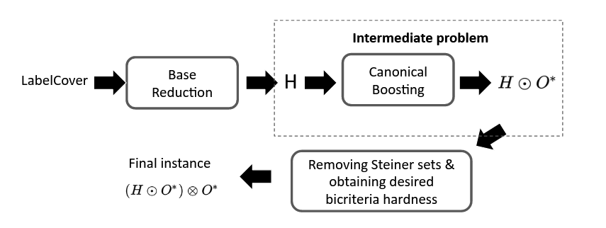
Figure 1: A high-level structure of our reduction. The boosting step handles the instances of the intermediate problem.

2.2 Upper Bound: An $(\alpha_{D},\alpha_{S})$-approximation algorithm

In this section, we give an overview of an approximately instance optimal shortcut (and TC-spanner) algorithm as mentioned in Theorem 1.2. Our goal is to find an $(\alpha_{D}d,\alpha_{S}s)$-shortcut in a given graph $G$ and integers $d$ and $s$ such that $G$ admits an $(d,s)$-shortcut. Our algorithm incorporates many ideas from the previous algorithm of [10]. Below, we present an overview and discuss how our techniques differ from theirs.

Denote by $\mathcal{P}\subseteq V(G)\times V(G)$ the (ordered) set of reachable pairs in $G$. The shortcut edges are chosen from $E^{T}\setminus E$ where $E^{T}$ are the edges in the transitive closure of $G$. We say that $F\subseteq(E^{T}\setminus E)$ $d^{\prime}$-settles the pair $(u,v)$ if the distance between them in $E\cup F$ is at most $d^{\prime}$. Therefore, to get $(\alpha_{D},\alpha_{S})$-approximation, it suffices to compute a subset $F\subseteq E^{T}\setminus E$ so that every pair in $\mathcal{P}$ is $(\alpha_{D}\cdot d)$-settled by $F$. We will handle two types of pairs in $\mathcal{P}$ separately. We say that $(u,v)\in\mathcal{P}$ is thick if the total number of vertices $w$ that are reachable from $u$ and can reach $v$ is at least $\beta$; otherwise, the pair $(u,v)$ is thin. Intuitively, a thick pair is “very well connected”. Divide $\mathcal{P}$ into $\mathcal{P}=\mathcal{P}_{thick}\cup\mathcal{P}_{thin}$.

The high-level ideas in dealing with these cases roughly follow [10]. At a high-level, a generic approach to turn a (single-criteria) approximation algorithm into a bicriteria one is to prove a certain “scaling advantage” result, e.g., proving that a $(1,\alpha_{S})$-approximation implies $(\alpha_{D},O(\alpha_{S}/\alpha_{D}))$-approximation (so when $\alpha_{D}=1$, we achieve roughly the same result).

Settling thick pairs.

Sample $V^{\prime}\subseteq V(G):|V^{\prime}|=\tilde{\Theta}(n/\beta)$ uniformly. For each sampled vertex $v\in V^{\prime}$, add edges from $v$ to all $v^{\prime}$ such that $v^{\prime}$ is reachable from $v$ or can reach $v$. Denote by $F_{1}$ the set of edges that are added by this process, so $|F_{1}|=\tilde{\Theta}(n^{2}/\beta)$. It is easy to see (via a hitting set argument) that, with constant probability, this set of shortcut edges reduces the diameter to two and the total number of shortcut edges is at most $\tilde{O}(n^{2}/\beta)$.

This simple sampling strategy has already been explored by [10] in the context of spanner construction. To incorporate the scaling advantage, we adapt the technique used in a recent paper demonstrating how to construct an $(\widetilde{O}(n^{1/3}),n)$-shortcut for any graph [42]. This adaptation reduces the size of the shortcut set to $\tilde{O}\left(n^{2}/\beta(\alpha_{D}d)^{2}\right)$ while still ensuring that the endpoints of all thick edges have a distance of at most $\alpha_{D}d$.

Settling the thin pairs.

Thin pairs are handled via LP-rounding techniques. We say that a set $A\subseteq E^{T}\backslash E$ is $d^{\prime}$-critical for thin pair $(u,v)\in\mathcal{P}_{thin}$ if in $E^{T}\setminus A$, the distance from $u$ to $v$ is larger than $d$; in other words, not taking any edge from $A$ would make the solution infeasible. Denote by $\mathcal{A}_{d^{\prime}}$ the set of all minimal and $d^{\prime}$-critical edges. Our definition of critical set is analogous to the notion of antispanners in [10]. The following claim is intuitive: It asserts an alternative characterization of shortcuts as a set of edges that hit every critical set.

Claim 2.1 (Adapted from [10]).

An edge set $E^{\prime}$ is a $d^{\prime}$-shortcut set for all thin pairs if and only if $E^{\prime}\cap A\neq\emptyset$ for all $A\in\mathcal{A}_{d^{\prime}}$.

The above claim allows us to write the following LP constraints for finding a $(d,s)$-shortcut.

$$\text{(LP)}:\qquad\sum_{e\in E^{T}\backslash E}x_{e} \leq s$$

$$\sum_{e\in A}x_{e} \geq 1\qquad\forall A\in\mathcal{A}_{d}$$

$$x_{e} \geq 0\qquad\forall e\in E^{T}\setminus E$$

Each variable $x_{e}$ indicate whether edge $e\in E^{T}\setminus E$ is included into the shortcut solution. Each constraint $\sum_{e\in A}x_{e}\geq 1$ asserts that critical edge set $A$ must be “hit” by the solution. There can be exponentially many constraints, but an efficient separation oracle exists, as we sketch below.

The high-level idea of [10] (when translated into our setting) is a “round-or-cut” procedure that, from a feasible solution $\textbf{x}\in[0,1]^{E^{T}\setminus E}$, randomly computes $F_{2}\subseteq E^{T}\setminus E$ of size $O(\beta s)$ that either (i) successfully $d$-settles all thin pairs in $\mathcal{P}_{thin}$ or (ii) can be used to find a critical set $A\in\mathcal{A}_{d}$ such that $\sum_{e\in A}x_{e}<1$. If Case (i) happens, we have successfully computed the solution $F_{2}$. Otherwise, when Case (ii) happens, we have a separation oracle. In order to incorporate the scaling advantage into this algorithm, we prove a decomposition lemma (Lemma C.14) which asserts that each $(\alpha_{D}\cdot d)$-critical set $A\in\mathcal{A}_{\alpha_{D}d}$ can be partitioned into $\alpha_{D}$ sets in $\mathcal{A}_{d}$, and such decomposition can be computed efficiently. This decomposition lemma allows us to generalize [10] to the bicriteria setting, leading to the set of size $O(\beta s/\alpha_{D})$ that $(\alpha_{D}d)$-settles thin pairs.

The full proofs are deferred to the appendix.

Appendix A Preliminaries

Graph terminology.

Given a directed graph (digraph) $G=(V,E)$, a directed edge, denoted by an ordered pair of vertices $(u,v)\in E$, is called an in-edge for $v$ and an out-edge for $u$. The vertices $u$ and $v$ are called the endpoints of the edge $(u,v)$. The out-degree of a node $u\in V$ denotes the number of out-edges $(u,v)\in E$, and the in-degree denotes the number of in-edges $(v,u)\in E$. The maximum in-degree and out-degree of $G$ are the highest in-degree and out-degree values among all nodes, respectively.

A path $p$ of length $\ell$ is a vertex sequence $(v_{0},v_{1},...,v_{\ell})$ where $(v_{i},v_{i+1})\in E$ for any $0\leq i<\ell$. The following phrases are equivalent and used interchangeably: $p$ is a path from $v_{0}$ to $v_{\ell}$, $v_{0}$ has a path to $v_{\ell}$, $v_{0}$ can reach $v_{\ell}$, $v_{\ell}$ is reachable from $v_{0}$, and $(v_{0},v_{\ell})$ is a reachable (ordered) pair. The distance between a pair of vertices $(v_{0},v_{\ell})$ is defined as the minimum length of paths from $v_{0}$ to $v_{\ell}$, denoted by $\text{dist}_{G}\left(v_{0},v_{\ell}\right)$. The diameter of graph $G$ is defined as the maximum distance between any two reachable vertex pairs.

Given a digraph $G$, we use $G^{T}=(V,E^{T})$ to represent the transitive closure of $G$. In other words, $(u,v)\in E^{T}$ if and only if vertex $u$ can reach vertex $v$ in $G$. For an edge $(u,v)\in E$, vertices $u$ and $v$ are referred to as the endpoints of the edge $(u,v)$. A subgraph of $G$ is a graph $G^{\prime}=(V^{\prime},E^{\prime})$, where $E^{\prime}\subseteq E$ and $V^{\prime}$ contain all vertices that are endpoints of edges in $E^{\prime}$. We will slightly stretch the terminology and use $E^{\prime}$ to also denote the subgraph $G^{\prime}$. For a given set of vertices $V^{\prime}\subseteq V$, the subgraph induced by $V^{\prime}$ is denoted by $G[V^{\prime}]$.

A.1 Shortcut and TC spanner

We first introduce the definition of TC spanner.

Definition A.1 (TC spanner).

For a digraph $G=(V,E)$, any subset of edges $E^{\prime}\subseteq E^{T}\backslash E$ that have the same transitive closure of $G$ is called a TC spanner of $G$. If $E^{\prime}$ has diameter at most $d$ and size at most $s$, we call $E^{\prime}$ as $(d,s)$-TC spanner.

The following problem is about TC spanner approximation.

Definition A.2 ($(\alpha_{D},\alpha_{S})$-MinTC).

Given a directed graph $G$ and integers $d$ and $s$, such that $G$ admits a $(d,s)$-TC spanner, the goal is to find a $(\alpha_{D}d,\alpha_{S}s)$-TC spanner.

Definition A.3 (Shortcut).

For a digraph $G=(V,E)$, any subset of edges $E^{\prime}\subseteq E^{T}$ is called a shortcut of $G$. For $s,d\in\mathbb{N}$, we say $E^{\prime}$ is a $(d,s)$-shortcut of $G$ if $|E^{\prime}|\leq s$ and the diameter of $E\cup E^{\prime}$ is at most $d$.

The following problem is about shortcut approximation.

Definition A.4 ($(\alpha_{D},\alpha_{S})$-MinShC).

Given a directed graph $G$ and integers $d$ and $s$, such that $G$ admits an $(d,s)$-shortcut, the goal is to find an $(\alpha_{D}d,\alpha_{S}s)$-shortcut.

When we write $\alpha_{S},\alpha_{D}$ as a function of $n$, the variable $n$ corresponds to the number of nodes present in graph $G$.

A.2 Reductions between Shortcut and TC spanner

In this section, we prove an approximate equivalence between the two problems.

Lemma A.5.

If there is a polynomial time algorithm solving $(\alpha_{D},\alpha_{S})$-MinShC, then there is a polynomial time algorithm solving $(\alpha_{D},\alpha_{S}+1)$-MinTC.

Proof.

Given a graph $G$ that admits a $(d,s)$-TC spanner, we will show how to find a $(\alpha_{D}d,(\alpha_{S}+1)s)$-TC spanner.

According to Theorem 1 [6], a unique subgraph $H$ exists such that deleting any edge of $H$ will make the transitive closure of $G^{T}$ and $H$ unequal. Therefore, we can find $H$ in polynomial time: start with $G^{T}$, and repeatedly delete edges if deleting an edge will not change the transitive closure until no edge can be deleted. Since $G$ admits a $(d,s)$-TC spanner, and a TC spanner must have the same transitive closure as $G$, we have $|E(H)|\leq s$.

After finding $H$, we use the $(\alpha_{D},\alpha_{S})$-shortcut algorithm with input $H$ and $s,d$ to find a $(\alpha_{D}d,\alpha_{S}s)$-shortcut $E^{\prime}$. $H$ admits a $(d,s)$-shortcut because the $(d,s)$-TC spanner of $G$ is also a $(d,s)$-shortcut of $H$. We claim that the graph $(V(H),E^{\prime}\cup E(H))$ is a $(\alpha_{D}d,(\alpha_{S}+1)s)$-TC spanner. According to the definition of shortcut, $(V(H),E^{\prime}\cup E(H))$ has a diameter at most $\alpha_{D}d$. The size is at most $\alpha_{S}s+|E(H)|\leq(\alpha_{S}+1)s$ since $|E(H)|\leq s$.

∎

Lemma A.6.

If there is a polynomial time algorithm solving $(\alpha_{D},\alpha_{S})$-MinTC, then there is a polynomial time algorithm solving $(\alpha_{D},2\alpha_{S})$-MinShC with input $s$ restricted to $s\geq m$.

Proof.

Given a graph $G$ with $m$ edges and $s\geq m,d$ such that $G$ admits a $(d,s)$-shortcut, we will show how to find a $(\alpha_{D}d,2\alpha_{S}s)$-shortcut.

We first prove that $G$ admits a $(d,2s)$-TC spanner. Let the $(d,s)$-shortcut of $G$ be $E^{\prime}$, then $E^{\prime}\cup E$ has size at most $2s$ since $s\geq m$, and has diameter $d$. Thus, $E^{\prime}\cup E$ is a $(d,2s)$-TC spanner of $G$.

We apply the $(\alpha_{D},\alpha_{S})$-MinTC algorithm on $G$ with inputs $2s,d$ to get a $(\alpha_{D}d,2\alpha_{S}s)$-TC spanner, which is also a $(\alpha_{D}d,2\alpha_{S}s)$-shortcut.

∎

A.3 Label cover and PGC.

In this section, we introduce the label cover problem and state the projection game conjecture formally.

Definition A.7 (LabelCover).

The LabelCover problem takes as input an instance $\mathcal{I}=(A,B,E,\mathcal{L},$ $(\pi_{e})_{e\in E})$ described as follows:

• $(A\cup B,E)$ is a bipartite regular graph with partitions $|A|=|B|$,

• a label set $\mathcal{L}$ and an non-empty acceptable label pair associated with each each $e=(u,v)\in E$ denoted by $\pi_{e}\subseteq\mathcal{L}\times\mathcal{L}$.

A labeling $\psi:V\to{\mathcal{L}}$ is a function that gives a label to each vertex $\psi(v)\in\mathcal{L}$. $\psi$ is said to cover an edge $e=(u,v)\in E$ if $(\psi(u),\psi(v))\in\pi_{e}$. The goal of the problem is to find a labeling that covers the most number of edges.

Conjecture A.8 (PGC).

There exists a universal constant $\epsilon>0$ such that, given a LabelCover instance on input of size $N$, it is hard to distinguish between the following two cases:

• (Completeness:) There is a labeling that covers every edge.

• (Soundness:) Any labeling covers at most $N^{-\epsilon}$ fraction of the edges.

We will use a slightly stronger hardness result where the soundness case is allowed to assign multiple labels. The hardness of this variant is a simple implication of the PGC. A multilabeling $\psi:V\to 2^{\mathcal{L}}$ gives a set of labels $\psi(v)\subseteq\mathcal{L}$ to a vertex $v$. Such a multilabeling is said to cover an edge $e=(u,v)\in E$ if there exists $a\in\psi(u),b\in\psi(v)$ such that $(a,b)\in\pi_{e}$. The cost of $\psi$ is denoted by $\sum_{u\in A\cup B}|\psi(u)|$. Notice that a valid labeling is a multi-labeling of cost $|A|+|B|$.

Lemma A.9.

Assuming PGC, there exists a sufficiently small constant $\epsilon_{L}{}>0$ such that, given a LabelCover instance of size $N$, there is no randomized polynomial time algorithm that distinguishes betweehn the following two cases:

• (Completeness:) There is a labeling that covers every edge.

• (Soundness:) Any multilabeling of cost at most $N^{\epsilon_{L}{}}(|A|+|B|)$ covers at most $N^{-\epsilon_{L}{}}$ fraction of edges.

Proof.

Suppose there is an algorithm that can distinguish the two cases described in Lemma A.9, we will show that it also distinguishes the two cases in Conjecture A.8. Completeness in Conjecture A.8 trivially implies completeness in Lemma A.9, we only need to show that it also holds for soundness. In other words, we want to show that if there exists a multilabeling $\phi$ of cost at most $N^{\epsilon_{L}}(|A|+|B|)$ that covers more than $N^{-\epsilon_{L}}$ fraction of edges for sufficiently small constant $\epsilon_{L}$, then there exists a labeling $\phi^{\prime}$ that covers more than $N^{-\epsilon}$ fraction of edges.

To construct $\phi^{\prime}$, we uniformly at random sample $1$ label from $\phi(v)$ for every $v\in A\cup B$ as the label $\phi^{\prime}(v)$. For each edge $(u,v)$ covered by $\phi$, the probability that $(u,v)$ is covered by $\phi^{\prime}$ is at least $1/(|\phi(u)|\cdot|\phi(v)|)$. Let $P$ contain all edges $(u,v)$ covered by $\phi$ such that $|\phi(u)|<N^{3\epsilon_{L}}$ and $|\phi(v)|<N^{3\epsilon_{L}}$. Since $\sum_{u\in A\cup B}|\phi(u)|\leq N^{\epsilon_{L}}(|A|+|B|)$, the number of nodes $u\in A\cup B$ that $|\phi(u)|\geq N^{3\epsilon_{L}}$ is bounded by $(|A|+|B|)/N^{2\epsilon_{L}}$. Remember that the bipartite graph is regular, so the number of edges $(u,v)$ with $|\phi(u)|\geq N^{3\epsilon_{L}}$ or $|\phi(v)|\geq N^{3\epsilon_{L}}$ is at most

$$\frac{2|E|}{|A|+|B|}\cdot\frac{|A|+|B|}{N^{2\epsilon_{L}}}=\frac{2|E|}{N^{2\epsilon_{L}}}$$

Since the number of edges covered by $\phi$ is at least $N^{-\epsilon_{L}}|E|$, we have

$$|P|\geq\frac{|E|}{N^{\epsilon_{L}}}-\frac{2|E|}{N^{2\epsilon_{L}}}\geq\frac{|E|}{N^{2\epsilon_{L}}}$$

The expectation of the number of covered edges by $\phi^{\prime}$ is at least

$$\sum_{(u,v)\in P}\frac{1}{|\phi(u)|\cdot|\phi(v)|}\geq\frac{|E|}{N^{8\epsilon_{L}}}$$

By setting $\epsilon_{L}<\epsilon/8$, the expectation is at least $\frac{|E|}{N^{\epsilon}}$, which means there must exists a labeling $\phi$ that covers more than $N^{-\epsilon}$ fraction of edges. ∎

A.4 Main Results

We restate the main results in the introduction in a formal way.

Theorem A.10 (Lower bound).

Under PGC, there exists a small constant $\epsilon>0$, such that no polynomial-time algorithm exists for solving $(n^{\epsilon},n^{\epsilon})$-MinShC as well as $(n^{\epsilon},n^{\epsilon})$-MinTC, even if we restricted the input $s=\Omega(m^{1+\epsilon}),d=\Omega(n^{\epsilon})$.

Recall that the Las Vegas algorithm is one that either generates a correct output or, with probability at most $1/2$, outputs $\bot$ to indicate its failure.

Theorem A.11 (Upper bound).

There is a polynomial time Las Vegas algorithm solving $(\alpha_{D},\alpha_{S})$-MinShC whenever the inputs $G,s,d$ satisfy the following conditions.

1. $s\geq|V(G)|$ and

2. $\alpha_{S}\geq\frac{Cn\log^{2}n}{\sqrt{sd^{2}\alpha_{D}^{3}}}$ for sufficiently large constant $C$.

Moreover, if we further require $\alpha_{S}\geq 2$, then there is a polynomial time Las Vegas algorithm solving $(\alpha_{D},\alpha_{S})$-MinTC.

Notice that the upper bound result is stated here in a slightly different form, as this form will be more convenient to derive formally. It is easy to show that Theorem A.11 implies $(n^{\gamma_{D}},n^{\gamma_{S}})$-approximation for $3\gamma_{D}+2\gamma_{S}>1$ (using the fact that $s\geq n$ and $d\geq 1$.)

Appendix B Lower Bounds

This section contains three parts.

In Section B.1, we will prove that there is no polynomial algorithm solving $(1,n^{\epsilon})$-MinShC. The technique is similar to the construction used by Elkin and Peleg [25] to prove the hardness of approximating directed spanner. We will also define MinStShC, as discussed in Section 2, and prove the hardness for MinStShC when $s=o(m)$.

In Section B.2, we will show how to prove the lower bound for $(n^{\epsilon},n^{\epsilon})$-MinShC, using the lower bound for MinStShC while preserving the relative size of $s$ versus $m$. It will only prove that $(n^{\epsilon},n^{\epsilon})$-MinShC is hard for some input $s=o(m)$ by combining with the result in Section B.1, which is still not what we want in Theorem A.10.

In Section B.3, we boost $s$ to be $\omega(m)$ in the lower bound proof of MinStShC. Combined with the lemma proved in Section B.2, this will show us $(n^{\epsilon},n^{\epsilon})$-MinShC is hard for some input $s=\Omega(m^{1+\epsilon})$, which is what we want in Theorem A.10.

B.1 Warm up: Lower Bounds when $\alpha_{D}=1$

This section will use a simple construction to prove the following lemma.

Lemma B.1.

Assuming PGC (Conjecture A.8), there are no polynomial time algorithm solving $(1,n^{\epsilon})$-MinShC for some small constant $\epsilon$.

The construction relies on the following LabelCover graph.

Definition B.2 (LabelCover graph).

Given a LabelCover instance $\mathcal{I}=(A,B,E,\mathcal{L},(\pi_{e})_{e\in E})$ descirbed in Definition A.7 and a parameter $\rho$, we define the LabelCover graph $G_{\mathcal{I},\rho}$ as a directed graph defined as follows (see Figure 2):

• Suppose $A=\{1,...,|A|\},B=\{1,...,|B|\},\mathcal{L}=\{1,2,...,|\mathcal{L}|\}$. In $G_{\mathcal{I},\rho}$ we have vertices $\{a^{(i)}_{j},b^{(i)}_{j}\mid 1\leq i\leq|A|=|B|,1\leq j\leq|\mathcal{L}|\}$ and edges $\{(a^{(i)}_{j},b^{(i^{\prime})}_{j^{\prime}})\mid(i,i^{\prime})\in E,(j,j^{\prime})\in\pi_{(i,i^{\prime})}\}$.

• In addition, $G_{\mathcal{I},\rho}$ also contains vertices $\{a^{(i)},b^{(i)}\mid 1\leq i,j\leq|A|=|B|\}$, where $a^{(i)}$ has a directed path with length $\rho$ to each vertex in $\{a^{(i)}_{j}\mid 1\leq j\leq|\mathcal{L}|\}$ denoted by $\alpha^{(i)}_{j}$, the vertices along the path are $\{\alpha^{(i)}_{j}[k]\mid 1\leq k\leq\rho-1\}$; similarly, $b^{(i)}$ has a directed path with length $\rho$ from each vertex in $\{b^{(i)}_{j}\mid 1\leq j\leq|\mathcal{L}|\}$ denoted by $\beta^{(i)}_{j}$, the vertices along the path are $\{\beta^{(i)}_{j}[k]\mid 1\leq k\leq\rho-1\}$.

• Finally, we add edges $(\alpha^{(i)}_{j}[k],a^{(i)}),(b^{(i)},\beta^{(i)}_{j}[k]),(a^{(i)}_{j},a^{(i)})$, $(b^{(i)},b^{(i)}_{j})$ for any possible $i,j,k$.

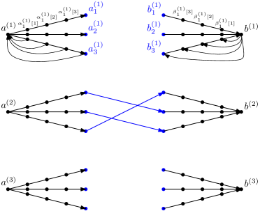
0.95

Figure 2: In this example, $|A|=|B|=|\mathcal{L}|=\rho-1=3$. Suppose $A=\{1,2,3\},B=\{1,2,3\},\mathcal{L}=\{1,2,3\}$, then in this example we have $E=\{(2,2)\}$ and $\pi_{(2,2)}=\{(1,2),(2,3),(3,1)\}$, which corresponds to the three edges in the middle.

Proof of Lemma B.1.

Given a LabelCover instance $\mathcal{I}=(A,B,E,\mathcal{L},(\pi_{e})_{e\in E})$, we use $\Delta$ to denote the size of $A$ (and also $B$). We now describe how to distinguish between the case. Notice that $N$ is the input size of the LabelCover instance $\mathcal{I}$.

• (Completeness:) There is a labeling that covers every edge.

• (Soundness:) Any multilabeling of cost at most $N^{\epsilon_{L}{}}(|A|+|B|)$ covers at most $N^{-\epsilon_{L}{}}$ fraction of edges.

According to Lemma A.9, this violates PGC.

If $|E|\leq 2\Delta n^{\epsilon_{L}}$, then it cannot be the Soundness case, so we assume $|E|>2\Delta n^{\epsilon_{L}}$.

First, we use polynomial time to compute the LabelCover graph $G_{\mathcal{I},\mathcal{\rho}{}}$ with $n$ vertices, where $\mathcal{\rho}{}$ is polynomial on $N$ and can be arbitrarily large. Then We run the $(1,n^{\epsilon})$-MinShC algorithm with input $G_{\mathcal{I},\mathcal{\rho}{}}$ and parameters $s=2\Delta,d=\mathcal{\rho}{}+1$. We will prove the following two claims, which will lead to the solution to the LabelCover problem.

Claim B.3.

If the LabelCover instance is in case (completness), then $G_{\mathcal{I},\mathcal{\rho}{}}$ has a $(\mathcal{\rho}{}+1,2\Delta)$-shortcut. Moerover, for any $(i,j)\in E$, $(a^{(i)},b^{(j)})$ has distance at most $3$ after adding this shortcut.

Proof.

Suppose the labeling is $\psi$. For any $i\in A$, we include the edge $(a^{(i)},a^{(i)}_{\psi(i)})$ in the shortcut; for any $i\in B$, we include the edge $(b^{(i)}_{\psi(i)},b^{(i)})$ in the shortcut. The shortcut has size $2\Delta$. Since $(i,j)$ is covered by $\psi$, there exists an edge $(a^{(i)}_{i^{\prime}},b^{(j)}_{j^{\prime}})$ such that $i^{\prime}=\psi(i),j^{\prime}=\psi(j)$. In that case, we have the length 3 path $(a^{(i)},a^{(i)}_{i^{\prime}},b^{(j)}_{j^{\prime}},b^{(j)})$ after adding the shortcut. This proves the second statement of this lemma. Now we verify the distances between reachable pairs are at most $\mathcal{\rho}{}+1$ one by one.

1. (start from $a^{(i)}$) $a^{(i)}$ can reach any $a^{(i)}_{j},\alpha^{(i)}_{j}[k]$ with distance at most $\mathcal{\rho}{}$, $a^{(i)}$ can reach any $b^{(j)}$ with $(i,i^{\prime})\in E$ with distance $3$, which means $a^{(i)}$ can reach any $\beta^{(i^{\prime})}_{j}[k],b^{(i^{\prime})}_{j}$ with distance $4$.

2. (start from $\alpha^{(i)}_{j}[k],a^{(i)}_{j}$) $\alpha^{(i)}_{j}[k]$ or $a^{(i)}_{j}$ has an edge to $a^{(i)}$, so they can reach any node that $a^{(i)}$ can reach with distance at most $\mathcal{\rho}{}+1$.

3. (start from $\beta^{(i)}_{j}[k],b^{(i)}_{j},b^{(i)}$) These nodes can reach any reachable nodes with distance at most $\mathcal{\rho}{}+1$ in $G_{\mathcal{I},\mathcal{\rho}{}}$.

∎

Claim B.4.

If the LabelCover instance is in case (soundness), then $G_{\mathcal{I},\mathcal{\rho}{}}$ does not have a $(\mathcal{\rho}{}+1,2\Delta\cdot n^{\epsilon})$-shortcut for sufficiently small constant $\epsilon$. Moreover, by adding any shortcut with size at most $2\Delta\cdot n^{\epsilon}$, at most $o(1)$ fraction of pairs in $\{(a^{(i)},b^{(j)})\mid(i,j)\in E\}$ will have distance less than $\mathcal{\rho}{}+1$.

Proof.

Suppose $G_{\mathcal{I},\mathcal{\rho}{}}$ has a shortcut $E^{\prime}$ adding which reduces the diameter between $\Omega(1)$ fraction of pairs in $\{(a^{(i)},b^{(j)})\mid(i,j)\in E\}$ to less than $\mathcal{\rho}{}+1$. We will try to get a contradiction. We first use $E^{\prime}$ to build a multilabeling $\psi$ in the following way: for any $1\leq i\leq|A|$, we let $\psi(i)$ to be the set of vertices among $\{a^{(i)}_{j}\mid 1\leq j\leq\mathcal{L}\}$ that $a^{(i)}$ has distance at most $\mathcal{\rho}{}-1$ to after adding the shortcut.

$\psi$ covers more than $N^{-\epsilon_{L}}$ fraction of edges.

We first argue that $\psi$ covers $\Omega(1)$ fraction of the edges. Write $A_{i}=\{a^{(i)},a^{(i)}_{j},\alpha^{(i)}_{j}[k]\mid 1\leq j\leq\mathcal{L},1\leq k\leq\mathcal{\rho}{}-1\},B_{i}=\{b^{(i)},b^{(i)}_{j},\beta^{(i)}_{j}[k]\mid 1\leq j\leq\mathcal{L},1\leq k\leq\mathcal{\rho}{}-1\}$. For an edges $(i,j)\in E$ (recall that $E$ is the edge set in the LabelCover instance $\mathcal{I}$), we say it is crossed if there is an edge $(u,v)\in E^{\prime}$ with $u\in A_{i},v\in B_{j}$ in $E^{\prime}$. Remember that we assumed $|E|\geq\Delta\cdot N^{\epsilon_{L}{}}$, otherwise, the case (soundness) can never happen. Therefore, the number of crossed edges is at most $2\Delta\cdot n^{\epsilon}=o(|E|)$ for sufficiently small $\epsilon$. Now We prove that for any non-crossed edge $(i,j)\in E$ such that $(a^{(i)},b^{(j)})$ has distance less than $\mathcal{\rho}{}+1$ after adding $E^{\prime}$, $(i,j)$ is covered by $\psi$. If we can prove this, then at least $\Omega(1)$ fraction of edges in $E$ are covered. To prove this, notice that if $(i,j)$ is not covered, then consider the shortest path $p$ from $a^{(i)}$ to $b^{(j)}$ after adding the shortcut, we write the part where $p$ is inside $A_{i}$ as $p_{A}$, and the part where $p$ is inside $B_{j}$ as $p_{B}$. if both $p_{A},p_{B}$ has length at most $\mathcal{\rho}{}-1$, then $(i,j)$ is covered. Thus, one of $p_{A}$ or $p_{B}$ has length at least $\mathcal{\rho}{}$. Then we have $|p|=|p_{A}|+1+|p_{B}|\geq\mathcal{\rho}{}+1+1\geq\mathcal{\rho}{}+2$, which is a contradiction.

$\psi$ has cost at most $N^{\epsilon_{L}}(|A|+|B|)$.

Then we argue that $\sum_{u\in A\cup B}|\psi(u)|\leq|E^{\prime}|\leq 2\Delta\cdot n^{\epsilon}$ (which will give us $\sum_{u\in A\cup B}|\psi(u)|\leq N^{\epsilon_{L}{}}(|A|+|B|)$ for sufficiently small $\epsilon$). For a label $j\in\psi(i)$, we have $\text{dist}_{(V,E\cup E^{\prime})}\left(a^{(i)},a^{(i)}_{j}\right)<\mathcal{\rho}{}$. Thus, there exists a path $p=(v_{0},...,v_{\ell})$ from $a^{(i)}$ to $a^{(i)}_{j}$ with length at most $\mathcal{\rho}{}-1$. Let $p^{\prime}=(a^{(i)},\alpha^{(i)}_{j}[1],\alpha^{(i)}_{j}[2],...,a^{(i)}_{j})$. Let $k$ be the last index such that $v_{k}\not\in p^{\prime}$ and $v_{k+1}\in p^{\prime}$. Since $v_{\ell}$ in $p^{\prime}$ and the length of $p^{\prime}$ equals $\mathcal{\rho}{}$, such $k$ must exist. Since $(v_{k},v_{k+1})\not\in E$, we have $(v_{k},v_{k+1})\in E^{\prime}$. We call this edge $(v_{k},v_{k+1})$ a critical edge of $(i,j)$. For different $i$ and $j$ with $j\in\psi(i)$, they have different critical edges in $E^{\prime}$ because the corresponding $v_{k+1}$ is always different. Thus, $\sum_{u\in A\cup B}|\psi(u)|\leq|E^{\prime}|\leq 2\Delta\cdot n^{\epsilon}$.

∎

If the LabelCover instance is in case (completeness), by B.3, $G_{\mathcal{I},\mathcal{\rho}{}}$ admits a $(\mathcal{\rho}{}+1,2\Delta)$-shortcut, which means the output by the $(1,n^{\epsilon})$-MinShC algorithm will be a $(\mathcal{\rho}{}+1,2\Delta\cdot n^{\epsilon})$-shortcut; on the other hand, if the LabelCover instance is in case (soundness), by B.4, the output cannot be a $(\mathcal{\rho}{}+1,2\Delta\cdot n^{\epsilon})$-shortcut since $G_{\mathcal{I},\mathcal{\rho}{}}$ does not have one. Since checking whether the output is $(\mathcal{\rho}{}+1,2\Delta\cdot n^{\epsilon})$-shortcut or not is in polynomial time, LabelCover is solved in polynomial time.

∎

In the following definition, we will abstract all the necessary properties of graph $G_{\mathcal{I},d}$ in a black box that we are going to use to prove the hardness for $(n^{\epsilon},n^{\epsilon})$-MinShC.

Definition B.5.

For $1>\epsilon,c_{M}{}>0$, the $\epsilon$-MinStShC$\mid_{c_{M}{}}$ problem has inputs

1. a directed connected graph $G=(V,E)$ with $m$ edges, $n$ nodes and diameter polynomial on $m$, let the diameter be $d$,

2. two sets $L,R\subseteq V$ with $L\cap R=\emptyset$, where $|L|$ is polynomial on $m$,

3. a set of reachable vertex pairs $P\subseteq L\times R$,

4. a positive integer $s=\Omega(m^{c_{M}{}})$.

The problem asks to distinguish the following two types of graphs.

Type 1.

There exists a shortcut $E^{\prime}$ of $G$ with size $s$ such that all reachable pairs $(u,v)\in L\times R$ have distance $O(1)$ after adding $E^{\prime}$ to $G$.

Type 2.

By adding any shortcut with size $s\cdot n^{\epsilon}$, at most $o(1)$ fraction of the pairs in $P$ have distance at most $d/3$.

The following lemma shows that Figure 2 is a hard instance for $\epsilon$-MinStShC$\mid_{c_{M}{}}$.

Lemma B.6.

Under PGC (Conjecture A.8), there exist constants $\epsilon,c_{M}{}$ such that $\epsilon$-MinStShC$\mid_{c_{M}{}}$ cannot be solved in polynomial time.

Proof.

Given any LabelCover instance $\mathcal{I}=(A,B,E,\mathcal{L},\pi)$ (we write $|A|=\Delta$), we construct a $\epsilon$-MinStShC$\mid_{c_{M}{}}$ instance with the following inputs.

1. The graph is $G_{\mathcal{I},\mathcal{\rho}{}}$ (see Definition B.2) for $\mathcal{\rho}{}$ arbitrarily large such that $\mathcal{\rho}{}$ is polynomial on $N$ (the bit length of instance $\mathcal{I}$). $G_{\mathcal{I},d}$ has diameter $d=2\mathcal{\rho}{}+1$.

2. $L=\{a_{i}\mid 1\leq i\leq\Delta\},R=\{b_{i}\mid 1\leq i\leq\Delta\}$, clearly $|L|=|R|\leq m$ and $|L|$ is polynomial on $m$.

3. $P=\{(a_{i},b_{j})\mid(i,j)\in E\}$.

4. $s=|A|+|B|$, it is polynomial on $m$.

Now we prove that if we have a polynomial time algorithm to distinguish the two types of graphs as described in Definition B.5, then we can solve LabelCover in polynomial time.

If $\mathcal{I}$ is in case (completeness), according to B.3, by adding a shortcut with size $s=(|A|+|B|)$, all reachable pairs $(a_{i},b_{j})$ (with $(i,j)\in E$) has distance at most 3.

If $\mathcal{I}$ is in case (soundness), according to B.4, by adding a shortcut with size less than $s\cdot n^{\epsilon}$ for sufficiently small $\epsilon$, at most $o(1)$ fraction of pairs in $P$ has distance less than $(2d+1)/3<\mathcal{\rho}{}$. ∎

B.2 Lower Bound when $\alpha_{D}>1$ and $s=o(m)$

In this section, we prove the following lemma, which shows how to use the hardness of $\epsilon$-MinStShC$\mid_{c_{M}{}}$ to get lower bounds for $\alpha_{D}>1$.

Lemma B.7.

For any constant $1>\epsilon,c_{M}{}>0$, if there is no polynomial algorithm solving $\epsilon$-MinStShC$\mid_{c_{M}{}}$, then for sufficiently small constant $\gamma$, there is no polynomial algorithm solving $(n^{\gamma\epsilon},n^{\gamma\epsilon})$-MinShC even if the input is restricted to $s=\Omega(m^{1+\gamma(c_{M}{}-1)})$.

By combining Lemmas B.6 and B.7, we can get the following corollary. Notice that this corollary is not the same as Theorem A.10, since it does not restrict $s$ to be $\omega(m)$.

Corollary B.8.

Under PGC (Conjecture A.8), there is no polynomial algorithm solving $(n^{\epsilon},n^{\epsilon})$-MinShC for sufficiently small constant $\epsilon$.

The following geometric graph [37] is a crucial part of our proof for Lemma B.7. We say a graph $G=(V,E)$ is a $k$-layered directed graph if $V=V_{1}\uplus V_{2}\uplus...\uplus V_{k}$ ($V$ is partitioned into $V_{1},...,V_{k}$), such that for any edge $(u,v)\in E$, there exists $1\leq i<k$ and $u\in V_{i},v\in V_{i+1}$. $V_{i}$ is called the $i$-th layer of $G$.

Lemma B.9 (Section 2.2 [37]).

For any $\Delta\in\mathbb{N}^{+}$, for arbitrary constant $0<{c_{lrs}}{}<1$, we can compute in polynomial time a $\Delta^{c_{lrs}}$ layered graph $G=(V,E)$, a set of pairs $P$ and an indexing $I{}$ satisfying the following properties.

1. Each layer of $G$ contains $\tilde{\Theta}\left(\Delta^{10}\right)$ vertices and has a maximum in-degree and out-degree of at most $\Delta$. Let the first layer be denoted as $V_{1}=\{s_{1},s_{2},\dots,s_{K_{1}}\}$ and the last layer as $V_{2}=\{t_{1},t_{2},\dots,t_{K_{2}}\}$.

2. $P\subseteq[K_{1}]\times[K_{2}]$. For every $i\in[K_{1}]$, there are $\Omega(\Delta^{2})$ pairs $(i,j)\in P$. For every $(i,j)\in P$, there is a unique path from $s_{i}$ to $t_{j}$ in $G$, denoted by $p_{i,j}$. $p_{i,j}$ and $p_{i^{\prime},j^{\prime}}$ shares at most one edge for different pairs $(i,j)\not=(i^{\prime},j^{\prime})$.

3. The function $I{}$ assigns a value from $[\Delta]$ to each $(v,e)$ pair, where $e$ is either an in-edge or an out-edge of vertex $v$. For a given vertex $v$, $I{}$ assigns distinct values to its different in-edges, and similarly, $I{}$ assigns distinct values to its different out-edges. For any $(x,y)\in[\Delta]\times[\Delta]$, there exists $\Omega(\Delta^{10})$ paths $p_{i,j}$ (where $(i,j)\in P$) such that for any edge $(u,v)$ on $p_{i,j}$,

   • if $v$ is in the even layer, then $I{}[v,(u,v)]=x$,

   • if $u$ is in the even layer, then $I{}[u,(u,v)]=y$.

Proof of Lemma B.9.

The general idea is to use the graph described in Section 2.2 [37] with max degree $\Delta$, and cut the first $\Delta^{{c_{lrs}}{}}$ layers to get our disired graph. Readers are recommanded to read the construction in Section 2.2 [37], and the construction for Lemma B.9 is followed straightforwardly.

Let the graph $G_{1}\otimes G_{2}$ described in Section 2.2 [37] with parameters $d_{1}=d_{2}=2,r_{1}=\Delta^{3/2}$ be $G_{\Delta}$. $G_{\Delta}$ has $\Omega(\Delta)$ layers, where each layer has $\tilde{\Theta}\left(\Delta^{10}\right)$ vertices. The max in/out-degree is $\Delta$. We use the subgraph of $G_{\Delta}$ induced by the first $\Delta^{{c_{lrs}}{}}$ layers to get the desired graph described in Lemma B.9, denoted by $G^{\prime}_{\Delta}$. We construct $P$ in the following way. According to Section 2.2 [37], there exist $\Omega(\Delta^{12})$ Critical Pairs in $G_{\Delta}$ between the first and last laryer nodes where each of them has a unique path connecting them. We cut each unique path at the first $\Delta^{{c_{lrs}}{}}$ layers, resulting in $\Omega(\Delta^{12})$ pairs between the first and last layer in $G^{\prime}_{\Delta}$. Now we verify the properties of $P$ one by one.

1. In Section 2.2 [37], each critical pairs is $((a,b,0),(a+Dv,b+Dw,2D))$ for some $v,w\in\mathcal{V}_{2}(r_{1})$. There are $\Delta$ possible choices for $v$ or $w$. Thus, for every $a$, there are $\Omega(\Delta^{2})$ choices of $b$ such that $(a,b)\in P$.

2. If the path between $(a,b)\in P$ is not unique, then the path between two critical pair in $G_{\Delta}$ is also not unique.

3. Since every two path between two critical pairs in $G_{\Delta}$ share at most one edge according to Lemma 2.6 [37], our path segments in the first $\Delta^{{c_{lrs}}{}}$ layers also share at most one edge.

Now we construct $I{}$. We fix an order for the set $\mathcal{V}_{2}(r_{1})=\{w_{1},w_{2},...,w_{\Delta}\}$. Each node in the even layer $(a,b,i)$ has out-edges $\{(a+w_{j},b,i+1)\left((a,b,i),(a+w_{j},b,i+1)\right)\mid j\in[\Delta]\}$. $I{}$ assign index $j$ to the edge $\left((a,b,i),(a+w_{j},b,i+1)\right)$. $(a,b,i)$ has in-edges $\{\left((a,b-w_{j},i-1),(a,b,i)\right)\mid j\in[\Delta],b-w_{j}\in B_{2}(R_{1}+\left\lceil(i-1)/2\right\rceil r_{1})\}$. $I{}$ assign $j$ to the edge $\left((a,b-w_{j},i-1),(a,b,i)\right)$. Now for any $(x,y)\in[\Delta]\times[\Delta]$, we consider all the unique paths from $(a,b,0)$ to $(a+\Delta^{{c_{lrs}}{}}x,b+\Delta^{{c_{lrs}}{}}y,\Delta^{{c_{lrs}}{}}-1)$. All edges in this path is either $\left((a+ix,b+iy,2i),(a+(i+1)x,b+iy,2i+1)\right)$, which is the in-edge of $(a+(i+1)x,b+iy,2i+1)$ assigned as $x$, or $((a+(i+1)x,b+iy,2i+1)$,$(a+(i+1)x,b+(i+1)y,2i+2))$, which is the out-edge of $(a+(i+1)x,b+iy,2i+1)$ assigned as $y$. ∎

Now we are ready to prove the main lemma in this section.

Proof of Lemma B.7.

Suppose $\mathcal{A}$ is the polynomial time algorithm for $(n^{\gamma\epsilon},n^{\gamma\epsilon})$-MinShC where input must satisfy $s=\Omega(m^{1+\gamma(c_{M}{}-1)})$. Given a $\epsilon$-MinStShC$\mid_{c_{M}{}}$ instance $G_{inr},(L,R),P^{\prime},{s^{\prime}}$ (see Definition B.5, we use $G_{inr},P^{\prime},s^{\prime}$ instead of $P,s$ to avoid conflicting of notations), we will show how to use $\mathcal{A}$ as an oracle to solve it in polynomial time.

Definition of $G$.

Let $\Delta=|L|=|R|$, let $M$ denote the number of edges in $G_{inr}$ and let the diameter of $G_{inr}$ be $\rho{}$. We first construct a graph $G$ in the following way. Let the graph, pairs, and indexing described in Lemma B.9 with parameter $\Delta$ and sufficiently small constant ${c_{lrs}}$ be $G_{geo},P,I$. Without loss of generality, we assume $\Delta^{c_{lrs}}$ is odd. $G$ contains the following parts. See Figure 3 as an example.

0.95

Figure 3: Suppose the graph above is the graph $G_{geo}$ with $\Delta=2$ (notice that for ease of explanation, the graph does not satisfy properties described in Lemma B.9). The graph below shows how we substitute each node $v$ by $G_{v}$. If $v$ is in the even layer, then $G_{v}$ is a copy of $G_{inr}$; otherwise, if $v$ is not in the first or last layer, $G_{v}$ is a star graph.

1. (Substitute nodes in even layers by copies of $G_{geo}$) for each vertex $v$ in the even layers of $G_{geo}$, create a copy of graph $G_{inr}$, denoted as $G_{v}$ as part of $G$. Suppose $L=\{a_{1},...,a_{\Delta}\},R=\{b_{1},...,b_{\Delta}\}$ (remember that $L,R$ are inputs to $\epsilon$-MinStShC$\mid_{c_{M}{}}$). $a_{i}$ and $b_{i}$ are denoted by $a^{v}_{i},b^{v}_{i}$ in $G_{v}$.

2. (Substitute nodes in odd layers by star graphs) for each vertex $v$ in the odd layers except the first and last layer of $G_{geo}$, create vertices $s_{1},...,s_{\Delta},t_{1},...,t_{\Delta},v$, and create edges $(s_{1},v),,...,(s_{\Delta},v),(v,t_{1}),...,(v,t_{\Delta})$.

3. (Keep first and last layer) remember that $I$ is the input to $\epsilon$-MinStShC$\mid_{c_{M}{}}$. $G$ includes all nodes in the first and last layer of $G_{geo}$, denoted by $s_{1},s_{2},...,s_{K_{1}}$ and $t_{1},t_{2},...,t_{K_{2}}$.

4. (Edges connected different parts) for each edge $e=(u,v)$ in $G_{geo}$, create an edge $(b^{u}_{I{}[u,e]},a^{v}_{I{}[v,e]})$ in $G$. If $u$ is in the first layer or $v$ is in the last layer, just create edge $(u,a^{v}_{I{}[v,e]})$ or $(b^{u}_{I{}[u,e]},v)$ instead.

Remember that $G_{geo}$ has $\Delta^{{c_{lrs}}{}}$ layers, each with $\Delta^{10}$ vertices, and the max degree of $G_{geo}$ is $\Delta$. The number of edges $m$ in $G$ can be calculated as

$$m=\tilde{\Theta}\left(\Delta^{10+{c_{lrs}}{}}\cdot M\right)+\tilde{\Theta}\left(\Delta^{10+{c_{lrs}}{}}\cdot\Delta\right)+O(\Delta^{10+{c_{lrs}}{}}\cdot\Delta)=\tilde{\Theta}\left(\Delta^{10+{c_{lrs}}{}}\cdot(\Delta+M)\right)$$

Use $\mathcal{A}$ to solve $\epsilon$-MinStShC$\mid_{c_{M}{}}$.

After constructing $G$, we apply $\mathcal{A}$ on $G$ with parameter $s=\Delta^{10+{c_{lrs}}}\cdot{s^{\prime}},d=C\rho$ for sufficiently large constant $C$. We first argue that $s=\Omega(m^{1+\gamma(c_{M}{}-1)})$ for sufficiently small $\gamma$ so this is a valid input. Remember that ${s^{\prime}}$ is one of the inputs to $\epsilon$-MinStShC$\mid_{c_{M}{}}$ such that $s^{\prime}=\Omega(M^{c_{M}{}})$. Also remember in Definition B.5, we require $|L|=|R|=\Delta\leq M$ to be polynomial on $M$. Denote $M=\Delta^{c_{\Delta}}$. Then we have $m=\tilde{\Theta}\left(\Delta^{10+{c_{lrs}}{}+c_{\Delta}}\right)$ and $s=\Delta^{10+{c_{lrs}}{}+c_{\Delta}c_{M}{}}$. Now we have $s/m=\tilde{\Theta}\left(\Delta^{c_{\Delta}(c_{M}{}-1)}\right)$, where $\Delta^{c_{\Delta}}=m^{\gamma}$ for some constant $\gamma$. Thus, we have $s=\Omega(m^{1+\gamma(c_{M}{}-1)})$.

Remember that $\rho$ is the diameter of $G_{inr}$. According to Definition B.5, $\rho{}$ is polynomial on $M$. Let $\rho{}=M^{c_{D}}$. Remember our goal is to distinguish the following two types of $\epsilon$-MinStShC$\mid_{c_{M}{}}$ instances.

Type 1.

There exists a shortcut $E^{\prime}$ of $G_{inr}$ with size $O(s^{\prime})$ such that all reachable pairs $(u,v)\in L\times R$ have distance $O(1)$ after adding $E^{\prime}$ to $G_{inr}$.

Type 2.

By adding any shortcut with size ${s^{\prime}}\cdot M^{\epsilon}$, at most $o(1)$ fraction of the pairs in $P^{\prime}$ have distance at most $\rho{}/3$.

We prove the following two lemmas to show the output of $\mathcal{A}$ suffices to distinguish whether the $\epsilon$-MinStShC$\mid_{c_{M}{}}$ instance is in type 1 or type 2.

Lemma B.10.

If the $\epsilon$-MinStShC$\mid_{c_{M}{}}$ instance is type 1, then $G$ has a $(O(\rho{}),s=\Delta^{10+{c_{lrs}}}\cdot{s^{\prime}})$-shortcut.

Proof.

For each copy of $G_{inr}$ (denoted as $G_{v}$) in $G$, we add ${s^{\prime}}$ edges to the shortcut to make all reachable pairs $(a^{v}_{i},b^{v}_{j})$ have distance $O(1)$. The shortcut has size at most $\Delta^{10+{c_{lrs}}}\cdot{s^{\prime}}$. Consider a reachable $(u,v)$ in $G$, we first argue that they have distance $O(\rho{}+\Delta^{c_{lrs}})$ after adding the shortcut. To see this, notice that a path connecting $u,v$ can only be in the form of $(u,p_{1},p_{2},...,p_{\ell},v)$ where $p_{i}$ is a path inside $G_{v}$ for some $v$, and $\ell\leq\Delta^{{c_{lrs}}}$. Each $p_{i}$ with $1<i<\ell$ will be in the form $(a^{v}_{i},...,b^{v}_{j})$ for some $v,i,j$. Notice that $(a^{v}_{i},b^{v}_{j})$ has distance $O(1)$ after adding the shortcut if $v$ is in the even layer (if $v$ is in the odd layer then there is already an existing length 2 paths connecting $(a^{v}_{i},b^{v}_{j})$). Therefore, $u$ has distance $O(\rho{}+\Delta^{c_{lrs}})$ to $v$. Remember that $\rho{}=M^{c_{D}}=\Delta^{c_{\Delta}c_{D}}$. By setting ${c_{lrs}}{}<c_{\Delta}c_{D}$, the distance is at most $O(\rho{})$. ∎

Lemma B.11.

If the $\epsilon$-MinStShC$\mid_{c_{M}{}}$ instance is type 2, then $G$ has no $(n^{\gamma\epsilon}\rho{},n^{\gamma\epsilon}s)$-shortcut.

Proof.

Before we prove our lemma, we need to do some preparations. Remember that $P^{\prime}$ is the input to $\epsilon$-MinStShC$\mid_{c_{M}{}}$ such that for any $(x,y)\in P^{\prime}\subseteq[\Delta]\times[\Delta]$, $a^{v}_{x}$ can reach $b^{v}_{y}$ for any $v$. Also recall that according to Lemma B.9 item 3, for every $(x,y)\in P^{\prime}\subseteq[\Delta]\times[\Delta]$, in $G_{geo}$ there exists $\Omega(\Delta^{10})$ paths $p_{i,j}$ (which is the unique path connecting $s_{i},t_{j}$) that all edges $(u,v)$ in this path is the in-edge indexed by $I$ as $x$ of $v$ if $v$ is in the even layer, or the out-edge indexed by $I$ as $y$ of $u$ if $u$ is in the even layer. That means in $G$, there is a path from $s_{i}$ to $t_{j}$ in the form of $p^{\prime}_{i,j}=(s_{i},a^{v_{2,q_{2}}}_{x},...,b^{v_{2,q_{2}}}_{y},a^{v_{3,q_{3}}}_{x},...,b^{v_{3,q_{3}}}_{y},...,t_{j})$. We say $p^{\prime}_{i,j}$ covers vertices $v_{2,q_{2}},v_{3,q_{3}},...$ at $(x,y)$. Moreover, for $(i^{\prime},j^{\prime})\not=(i,j)$, we know from Lemma B.9 item 2 that $p_{i,j},p_{i^{\prime},j^{\prime}}$ shares at most one edge. Thus, $p^{\prime}_{i,j}$ and $p^{\prime}_{i^{\prime},j^{\prime}}$ cannot cover the same vertex $v$ at the same $(x,y)$, otherwise they share two edges: the in-edge indexed as $x$ of $v$ and the out-edge indexed as $y$ of $v$. In summary, we have $\Omega(\Delta^{10}|P^{\prime}|)$ pairs $(i,j)$, which we call critical pairs, satisfying the following properties.

1. $s_{i}$ can reach $t_{i}$ in $G$, where all paths from $s_{i}$ to $t_{i}$ must be in the form $(s_{i},a^{v_{2,q_{2}}}_{x},...,b^{v_{2,q_{2}}}_{y},a^{v_{3,q_{3}}}_{x},$ $...,b^{v_{3,q_{3}}}_{y},...,t_{j})$.

2. Any path from $s_{i}$ to $t_{j}$ cover one vertex $v$ in each layer at some pair $(x,y)\subseteq P^{\prime}$. For different critical pairs $(i,j)\not=(i^{\prime},j^{\prime})$, they will not cover the same vertex $v$ at the same pair $(x,y)\subseteq P^{\prime}$.

Now we are ready to prove Lemma B.11. We will prove that $G$ does not have a $(\rho{}\Delta^{{c_{lrs}}}/9,\Delta^{10+{c_{lrs}}}\cdot{s^{\prime}}\cdot M^{\epsilon/2})$-shortcut. We first show why this implies Lemma B.11. Remember that $s=\Delta^{10+{c_{lrs}}}\cdot{s^{\prime}}$, thus, $\Delta^{10+{c_{lrs}}}\cdot{s^{\prime}}\cdot M^{\epsilon/2}>m^{\gamma\epsilon}s)$ for sufficiently small constant $\gamma$. Also remember that $m$ is polynomial on $\Delta$, thus, $\rho{}\Delta^{{c_{lrs}}{}}/9>m^{\gamma\epsilon}\rho{}$ for sufficiently small constant $\gamma$.

Suppose to the contrary, $G$ has a $(\rho{}\Delta^{{c_{lrs}}}/9,\Delta^{10+{c_{lrs}}}\cdot{s^{\prime}}\cdot M^{\epsilon/2})$-shortcut, we will make a contradiction. We first claim that $G$ also has a $(\rho{}\Delta^{{c_{lrs}}}/8,\Delta^{10+{c_{lrs}}}\cdot{s^{\prime}}\cdot M^{\epsilon/2}\cdot\Delta^{{c_{lrs}}})$-shortcut, denoted by $E^{\prime}$, such that both end points for every edge in $E^{\prime}$ is in the same layer. We can achieve this by taking any edge $(u,v)$ in the original shortcut that crosses different layers, finding the path from $u$ to $v$ denoted by $p$, and cut $p$ into at most $\Delta^{c_{lrs}}$ segments $p_{1},p_{2},...,p_{\ell}$ where each segment is in the same layer, and replace $(u,v)\in E^{\prime}$ by $\Delta^{{c_{lrs}}}$ new edges each connecting two end points of $p_{i}$ from $i=1$ to $i=\ell$. In this way, the shortcut increase by a factor of at most $\Delta^{c_{lrs}}$. The distance between two vertices increases by at most an additive factor of $O(\Delta^{c_{lrs}})$. Another property of $E^{\prime}$ is that every edge in $E^{\prime}$ has both endpoints in $G_{v}$ for some $v$. That is because different $G_{v}$ where $v$ in the same layer are not reachable from each other.

Now with $E^{\prime}$ added to $G$, we denote the new graph by $G^{\prime}$. We define an indicator variable $I_{v,i,j}$ to be $1$ if $\text{dist}_{G^{\prime}}\left(a^{v}_{i},b^{v}_{j}\right)\leq\rho{}/3$. We know from the property of type 2 that for any $v$ and arbitrary small constant $\eta$, $\sum_{i,j\in P^{\prime}}I_{v,i,j}>\eta|P^{\prime}|$ implies $E^{\prime}$ has at least ${s^{\prime}}\cdot M^{\epsilon}$ edges in $G_{v}$. Since $|E^{\prime}|\leq\Delta^{10+{c_{lrs}}}\cdot{s^{\prime}}\cdot M^{\epsilon/2}\cdot\Delta^{{c_{lrs}}}$, by setting ${c_{lrs}}<1/2$, at most $o(\Delta^{10+{c_{lrs}}})$ vertices $v$ has the property that $\sum_{i,j\in P^{\prime}}I_{v,i,j}>\eta|P^{\prime}|$, which means $\sum_{v,(i,j)\in P^{\prime}}I_{v,i,j}\leq 2\eta\Delta^{10+{c_{lrs}}}|P^{\prime}|$. However, for each critical pair $(i,j)$, suppose $T_{i,j}=\{(v,x,y)\mid(i,j)\text{ covers }v\text{ at }(x,y)\}$, then we have $\sum_{(v,x,y)\in T_{i,j}}I_{v,x,y}\geq(1/2)\Delta^{c_{lrs}}$, otherwise the distance $\text{dist}_{G^{\prime}}\left(s_{i},t_{j}\right)$ with be at least $(\Delta^{c_{lrs}})/2\cdot\rho{}/3>\rho{}\Delta^{c_{lrs}}/6$. We also know that $T_{i,j}$ is disjoint for different $i,j$. Thus, we get $\sum_{v,i,j}I_{v,i,j}=\Omega(\Delta^{10}|P^{\prime}|)\cdot\Delta^{c_{lrs}}/2=\Omega(|P^{\prime}|\Delta^{10+{c_{lrs}}})$, contradicts the fact that $\sum_{v,i,j}I_{v,i,j}\leq 2\eta\Delta^{10+{c_{lrs}}}|P^{\prime}|$ for sufficiently small constant $\eta$.

∎

If the $\epsilon$-MinStShC$\mid_{c_{M}{}}$ instance is type 1, then according to Lemma B.10, $G$ admits a $(O(\rho{}),s=\Delta^{10+{c_{lrs}}}\cdot{s^{\prime}})$-shortcut, so $\mathcal{A}$ will output a $(n^{\gamma\epsilon}\rho{},n^{\gamma\epsilon}s)$-shortcut; on the other hand, if the $\epsilon$-MinStShC$\mid_{c_{M}{}}$ instance is type 2, then according to Lemma B.10, $G$ cannot output a $(n^{\gamma\epsilon}\rho{},n^{\gamma\epsilon}s)$-shortcut. Since checking whether an edge set is a $(n^{\gamma\epsilon}\rho{},n^{\gamma\epsilon}s)$-shortcut or not is in polynomial time, the output of $\mathcal{A}$ distinguish type 1 from type 2.

∎

B.3 Lower Bound when $\alpha_{D}>1$ and $s=\omega(m)$

In this section, we prove the following lemma.

Lemma B.12.

Assuming PGC (Conjecture A.8), there exists two constants $0<\delta,\epsilon<1$ such that $\epsilon$-MinStShC$\mid_{1+\delta}$ cannot be solved in polynomial time.

by combining Lemmas B.12 and B.7, we can get the proof of Theorem A.10.

Proof of Theorem A.10.

According to Lemma B.12, under PGC, there exists two constants $0<\delta,\epsilon<1$ such that $\epsilon$-MinStShC$\mid_{1+\delta}$ cannot be solved in polynomial time. According to Lemma B.7, there are no polynomial algorithm solving $(m^{\gamma\epsilon},m^{\gamma\epsilon})$-MinShC when input $s=\Omega(m^{1+\gamma(1+\delta-1)})=\Omega(m^{1+\gamma\delta})$ for some constant $\gamma$. ∎

Proof of Lemma B.12.

Given a LabelCover instance $\mathcal{I}=(A,B,E,\mathcal{L},(\pi_{e})_{e\in E})$ described in Definition A.7, PGC implies we cannot distinguish the following two cases in polynomial time for some small constant $\epsilon_{L}{}$ according to to Lemma A.9. Remember that $N$ is the input bit length of $\mathcal{I}$.

• (Completeness:) There is a labeling that covers every edge.

• (Soundness:) Any multilabeling of cost at most $N^{\epsilon_{L}{}}(|A|+|B|)$ covers at most $N^{-\epsilon_{L}{}}$ fraction of edges.

Assuming there is a polynomial time algorithm $\mathcal{A}$ solving $\epsilon$-MinStShC$\mid_{1+\delta}$ for sufficiently small constant $\epsilon$, we will show how to distinguish the above two cases in polynomial time, which will lead to a contradiction.

Definition of $G$.

First, we construct a graph $G$ (see Figure 4) according to the instance $\mathcal{I}$. Let $\Delta=N^{c_{\Delta}}$ for a sufficiently large constant $c_{\Delta}$. Denote the graph described by Lemma B.9 with parameter $\Delta$ as $G_{geo}$. Remember that $G_{geo}$ has $\Delta^{{c_{lrs}}{}}$ layers, each with size $\Theta(\Delta^{10})$, where the first layer is $S=\{s_{1},s_{2},...,s_{K_{1}}\}$, the last layer is $T=\{t_{1},t_{2},...,t_{K_{2}}\}$.

1. $G$ has two sides: $A$ side and $B$ side. Each side contains $K_{1}$ batches, each batch is composed by $|A|=|B|$ fans. Let the reversed graph of $G_{geo}$ (where we reverse all the edge directions in this graph) as $G^{R}_{geo}$. On the $A$ side, each fan is composed of $\mathcal{L}$ copies of graph $G^{R}_{geo}$; on the $B$ side, each is composed of $\mathcal{L}$ copies of a graph $G_{geo}$. All $G^{R}_{geo}$ or $G_{geo}$ in the same fan share the same $T$ vertex set. On the $A/B$ side, the $k$-th copied graph in the $i$-th batch, $j$-th fan is denoted by $G^{A/B}_{i,j,k}$, where the node $s_{\ell}$ in $G_{geo}$ is denoted by $s^{A/B}_{(i,j),\ell}$ for $1\leq\ell\leq K_{1}$ (recall that for different $k$, they share the same $s_{\ell}$), and the node $t_{\ell}$ in $G_{geo}$ is denoted by $t^{A/B}_{(i,j,k),\ell}$ for $1\leq\ell\leq K_{2}$.

2. $G$ has edges defined by the LabelCover instance $\mathcal{I}$ from $A$ side to $B$ side described as follows. Remember that $\mathcal{I}=(A,B,E,\mathcal{L},(\pi_{e})_{e\in E})$ where $A=\{1,2,...,|A|\},B=\{1,2,...,|B|\},\mathcal{L}=\{1,2,...,|\mathcal{L}|\}$. For every $(j,j^{\prime})\in E,(k,k^{\prime})\in\pi_{(j,j^{\prime})}$ and $i,\ell\in[K_{1}]$, there is an edge from $s^{A}_{(i,j,k),\ell}$ to $s^{B}_{(\ell,j^{\prime},k^{\prime}),i}$. An intuition of why the edges are defined in this way is that, now if a path is from the $A$ side of the $i$-th batch to $B$ side of the $\ell$-th batch, the path must go through $s^{A}_{(i,j,k),\ell}$ to $s^{B}_{(\ell,j^{\prime},k^{\prime}),i}$ for some $(j,j^{\prime})\in E,(k,k^{\prime})\in\pi_{(j,j^{\prime})}$.

3. For every $\ell\in[K_{2}]$, create a node $p^{A}_{\ell}$ and edges $\{(t^{A}_{(i,j),\ell},p^{A}_{\ell})\mid 1\leq i\leq K_{1},1\leq j\leq|A|)\}$. For every $i\in[K_{1}]$, create a node $q^{B}_{i}$ and edges $\{(q^{B}_{i},t^{B}_{(i,j),\ell})\mid 1\leq j\leq|A|,1\leq\ell\leq K_{2}\}$. Remember that in Lemma B.9, $P$ is a set of pairs between first and last layer indexes of nodes in $G_{geo}$. For every $\ell\in[K_{2}],i\in[K_{1}]$ where $(i,\ell)\not\in P$, we create an edge $(p^{A}_{\ell},q^{B}_{i})$.

   We also create a mirror of the above nodes and edges (Figure 4 does not draw) by reversing $A$ and $B$. i.e., for every $\ell\in[K_{2}]$, create a node $p^{B}_{\ell}$ with edges $\{(p^{B}_{\ell},t^{B}_{(i,j),\ell})\mid 1\leq i\leq K_{1},1\leq j\leq|A|)\}$. For every $i\in[K_{1}]$, create a node $q^{A}_{i}$ with edges $\{(t^{A}_{(i,j),\ell},q^{A}_{i})\mid 1\leq j\leq|A|,1\leq\ell\leq K_{2}\}$. For every $\ell\in[K_{2}],i\in[K_{1}]$ where $(i,\ell)\not\in P$, we create an edge $(q^{A}_{i},p^{B}_{\ell})$.

Remember that the number of edges in $G_{geo}$ is $M=O(\Delta^{11+{c_{lrs}}{}})$. Let $n$ be the number of nodes in $G$. Let $m$ be the number of edges in $G$. $m$ can be calculated as

$$m={\color[rgb]{.5,.5,.5}M\cdot K_{1}|A||\mathcal{L}|}+{\color[rgb]{0,0,1}O(|\mathcal{L}|^{2}|A|^{2})\cdot K_{1}^{2}}+{\color[rgb]{1,.5,0}4K_{1}K_{2}|A|}+{\color[rgb]{1,0,0}O(K_{1}K_{2})}=\Theta(M\cdot K_{1}|A||\mathcal{L}|)$$

The third and fourth terms are trivially less than the first term. The second term is less than the first term since we set $\Delta=N^{c_{\Delta}}$ for sufficiently large constant $c_{\Delta}$.

Figure 4: $G^{A}_{i,j,k}$ is one copy of the graph described in Lemma B.9 in the $i$-th batch (from right to left), $j$-th fan (from top to bottom) and $k$-th piece. For different $k$ and fixed $i,j$, $G^{A}_{i,j,k}$ shares the same first layer nodes (which are $s^{A}_{(i,j),\ell}$), but have different last layer nodes (which are $t^{A}_{(i,j,k),\ell}$). By changing $A$ to $B$ we get another side of the graph. Each dashed rectangle specifies the graph similar to the middle part in Figure 2 according to the input LabelCover instance $\mathcal{I}$. Fix $j,k$, for any $i,\ell$, we have $t^{A}_{(i,j,k),\ell}$ and $t^{B}_{(\ell,j,k),i}$ in the same dashed rectangle.

Solve LabelCover using $\epsilon$-MinStShC$\mid_{1+\delta}$

Now we run the $\epsilon$-MinStShC$\mid_{1+\delta}$ algorithm $\mathcal{A}$ with the following inputs. We need to verify that the inputs satisfy the requirements specified by Definition B.5.

1. Graph $G$ with $m$ edges. The diameter of $G$ is $d=2\Delta^{{c_{lrs}}{}}$, which is polynomial on $m$.

2. Two sets $L=\{t^{A}_{(i,j),k}\mid 1\leq i\leq K_{1},1\leq j\leq|A|,1\leq k\leq|\mathcal{L}|\},R=\{t^{B}_{(i,j),k}\mid 1\leq i\leq K_{1},1\leq j\leq|A|,1\leq k\leq|\mathcal{L}|\}$. The size of each set is $K_{1}|A||\mathcal{L}|$ which is polynomial on $m$.

3. A set of reachable vertex pairs $P^{\prime}\subseteq L\times R$ defined as follows. Recall that in the LabelCover instance, we have $A=\{1,...,|A|\},B=\{1,...,|B|\}$, and $P$ is the set of pairs defined in Lemma B.9. For every $i\in[K_{1}]$ let $I_{i}$ contain all indexes $x\in[K_{2}]$ such that $(i,x)\in P$. Let $I_{i}[\ell]$ be the $\ell$-th element in $I_{i}$. Now we define our $P^{\prime}$.

   $$P^{\prime}=\left\{\left(t^{A}_{(i,j),I_{i^{\prime}}[\ell]},t^{B}_{(i^{\prime},j^{\prime}),I_{i}[\ell]}\right)\mid 1\leq i,i^{\prime}\leq K_{2},(j,j^{\prime})\in E,1\leq\ell\leq\min(|I_{i^{\prime}}|,|I_{i}|)\right\}$$

   We need to argue that $P^{\prime}$ only contains reachable pairs. Notice that $t^{A}_{(i,j),I_{i^{\prime}}[\ell]}$ can reach $s^{A}_{(i,j,k),i^{\prime}}$ for any $k$ since $(i^{\prime},I_{i}[\ell])\in P^{\prime}$ (recall that $G^{A}_{(i,j,k)}$ is the reversed graph $G^{R}_{geo}$); for the same reason $t^{B}_{(i^{\prime},j^{\prime}),I_{i}[\ell]}$ can be reached from $s^{B}_{(i^{\prime},j^{\prime},k^{\prime}),i}$ for any $k^{\prime}$. Now we only need to argue that there exists $k,k^{\prime}$ such that $t^{A}_{(i,j,k),i^{\prime}}$ can reach $s^{B}_{(i^{\prime},j^{\prime},k^{\prime}),i}$. We can take the $(k,k^{\prime})\in\pi_{(j,j^{\prime})}$ where $\pi_{(j,j^{\prime})}$ must be non-empty since $(j,j^{\prime})\in E$.

Remember that the output of $\mathcal{A}$ will distinguish the following two types of instances.

Type 1.

There exists a shortcut $E^{\prime}$ of $G$ with size $O(m^{1+\delta})$ such that all reachable pairs $(u,v)\in L\times R$ have distance $O(1)$ after adding $E^{\prime}$ to $G$.

Type 2.

By adding any shortcut with size $O(m^{1+\delta+\epsilon})$, at most $o(1)$ fraction of pairs in $P$ have distance at most $d/3$.

Next we show the output can already distinguish the LabelCover instance (completeness) from (soundness).

(Completeness) implies Type 1.

Suppose the multilabeling covering all edges in (completeness) is $\psi$. Recall that $P^{\prime}$ is the pair set described in Lemma B.9. We create a shortcut $E^{\prime}$ defined as

$$E^{\prime} =\{(t^{A}_{(i,j),\ell},s^{A}_{(i,j,k),\ell^{\prime}})\mid i\in[K_{1}],j\in[|A|],k\in\psi(j),(\ell^{\prime},\ell)\in P^{\prime}\}$$

$$\cup\{(s^{B}_{(i,j,k),\ell},t^{B}_{(i,j),\ell^{\prime}})\mid i\in[K_{1}],j\in[|B|],k\in\psi(j),(\ell,\ell^{\prime})\in P^{\prime}\}$$

We have $|E^{\prime}|=O(K_{1}|A|\Delta^{12})$. Remember that $m=\Theta(M\cdot K_{1}|A||\mathcal{L}|)$, we have $|E^{\prime}|=\Theta(m^{1+\delta})$ for some constant $\delta$. Now we prove that all reachable pairs $(t^{A}_{(i,j),\ell},t^{B}_{(i^{\prime},j^{\prime}),\ell^{\prime}})$ has distance $O(1)$ after adding $E^{\prime}$. If $(i^{\prime},\ell)\not\in P$ or $(i,\ell^{\prime})\not\in P$, then $t^{A}_{(i,j),\ell}$ can reach $t^{B}_{(i^{\prime},j^{\prime}),\ell^{\prime}}$ in $3$ steps. Thus, we only consider the case when $(i^{\prime},\ell),(i,\ell^{\prime})\in P$. If $(j,j^{\prime})\not\in E$, then $(t^{A}_{(i,j),\ell},t^{B}_{(i^{\prime},j^{\prime}),\ell^{\prime}})$ is not reachable. Suppose $(j,j^{\prime})\in E$, let $k\in\psi(j),k^{\prime}\in\psi(j^{\prime})$, since $(j,j)$ is covered by $\psi$, there is a blue edge $(s^{A}_{(i,j,k),i^{\prime}},s^{B}_{(i^{\prime},j^{\prime},k^{\prime}),i})$. Besides, we have $(t^{A}_{(i,j),\ell},s^{A}_{(i,j,k),i^{\prime}}),(s^{B}_{(i^{\prime},j^{\prime},k^{\prime}),i},t^{B}_{(i^{\prime},j^{\prime}),\ell^{\prime}})\in E^{\prime}$ due to the fact that $(i^{\prime},\ell),(i,\ell^{\prime})\in P$. Thus, the distance between $(t^{A}_{(i,j),\ell},t^{B}_{(i^{\prime},j^{\prime}),\ell^{\prime}})$ is $3$.

(Soundness) implies Type 2.

We will prove it by contradiction. Suppose there exists a shortcut $E^{\prime}$ with size $O(m^{1+\delta+\epsilon})=O(K_{1}|A|\Delta^{12}\cdot n^{\epsilon})$, after adding which, not $o(1)$ fraction of pairs in $P$ have distance at most $d/3=(2/3)\Delta^{{c_{lrs}}{}}$. We first turn $E^{\prime}$ into another shortcut $E^{\prime\prime}$ where each shortcut in $E^{\prime\prime}$ is totally in a copy of graph $G_{geo}$ in the following way. Suppose $(u,v)\in E^{\prime}$ where $u,v$ are not in the same copy of $G_{geo}$, a path from $u$ to $v$ must cross at most two copies of $G_{geo}$, one on thie $A$ size and another on the $B$ size. We split this path into the two copies, and creat two edges connected two end points of both path . $E^{\prime\prime}$ will have size twice of $E^{\prime}$, and the distance after adding $E^{\prime\prime}$ will be at most $(2/3)\Delta^{{c_{lrs}}{}}+2$.

Recall that for every $i\in[K_{1}]$, we defined $I_{i}$ as all indexes $x\in[K_{2}]$ such that $(i,x)\in P$. We create multilabeling $\psi_{i,i^{\prime},\ell}$ in the following way: for every $j\in A,j^{\prime}\in B$, we let

$$\psi_{i,i^{\prime},\ell}(j)=\left\{k\in\mathcal{L}\mid\text{dist}_{G+E^{\prime\prime}}\left(t^{A}_{(i,j),I_{i^{\prime}}[\ell]},s^{A}_{(i,j,k),i^{\prime}}\right)<\Delta^{{c_{lrs}}{}}\right\}$$

$$\psi_{i,i^{\prime},\ell}(j)=\left\{k\in\mathcal{L}\mid\text{dist}_{G+E^{\prime\prime}}\left(s^{B}_{(i^{\prime},j,k),i},t^{B}_{(i^{\prime},j),I_{i}[\ell]}\right)<\Delta^{{c_{lrs}}{}}\right\}$$

One importance observation is, for every $\psi_{i,i^{\prime},\ell}$ and $k\in\mathcal{L}$, there is a unique path from $t^{A}_{(i,j),I_{i^{\prime}}[\ell]}$ to $t^{A}_{(i,j,k),i^{\prime}}$ or from $s^{B}_{(i^{\prime},j^{\prime},k),I_{i}[\ell]}$ to $t^{B}_{(i^{\prime},j^{\prime}),\ell}$; any two of these unique paths shares at most one edge. The reason is $(i,I_{i}[\ell])\in P$ (see Lemma B.9). As a result, each edge in $E^{\prime\prime}$ can make at most one pair of vertices $(t^{A}_{(i,j),I_{i^{\prime}}[\ell]},s^{A}_{(i,j,k),i^{\prime}})$ or $(s^{B}_{(i^{\prime},j,k),i},t^{B}_{(i^{\prime},j),I_{i}[\ell]})$ to have distance less that the original distance $\Delta^{{c_{lrs}}{}}$. Therefore,

$$\sum_{i,i^{\prime}\in[K_{1}],\ell\leq\min(|I_{i^{\prime}}|,|I_{i}|)}\left(|\psi_{i,i^{\prime},\ell}(j)|+|\psi_{i,i^{\prime},\ell}(j)|\right)\leq|E^{\prime\prime}|=O(K_{1}|A|\Delta^{12}\cdot n^{\epsilon})$$

According to Lemma B.9, we know $\min(|I_{i^{\prime}}|,|I_{i}|)=\Omega(\Delta^{2})$, which means the number of multilabeling $\psi_{i,i^{\prime},\ell}$ is $T=\Theta(K_{1}^{2}\Delta^{2})=\Theta(K_{1}\Delta^{12})$. Thus, only $o(K_{1}\Delta^{12})$ of them will have size at least $N^{\epsilon_{L}{}}(|A|+|B|)$ for sufficiently small constant $\epsilon$, where $N$ is the input size of $\mathcal{I}$ which is polynomial on $n$. Let $C(\psi_{i,i^{\prime},\ell})$ be the number of edges covered by $\psi_{i,i^{\prime},\ell}$ for instance $\mathcal{I}$. We have

$$\sum_{i,i^{\prime},\ell}C(\psi_{i,i^{\prime},\ell})\leq o(K_{1}\Delta^{12})\cdot|E|+T\cdot o(|E|)\leq o(T|E|)$$

One can see that if $\psi_{i,i^{\prime},\ell}$ does not cover an edge $(j,j^{\prime})$, then the distance from $t^{A}_{(i,j),I_{i^{\prime}}[\ell]}$ to $t^{B}_{(i^{\prime},j),I_{i}[\ell]}$ is at least $\Delta^{{c_{lrs}}{}}>(2/3)n^{c_{D}}$, where $(t^{A}_{(i,j),I_{i^{\prime}}[\ell]},t^{B}_{(i^{\prime},j),I_{i}[\ell]})\in P^{\prime}$. That is because the only path from $t^{A}_{(i,j),I_{i^{\prime}}[\ell]}$ to $t^{B}_{(i^{\prime},j),I_{i}[\ell]}$ must be the concatenation of paths between $t^{A}_{(i,j),I_{i^{\prime}}[\ell]},s^{A}_{(i,j,k),i^{\prime}}$ and between $s^{B}_{(i^{\prime},j,k^{\prime}),i},t^{B}_{(i^{\prime},j),I_{i}[\ell]}$ for some $k,k^{\prime}\in\mathcal{L}$, where at least one of them has length $\Delta^{{c_{lrs}}{}}$. Therefore, we have at least $(1-o(1))T|E|=(1-o(1))|P^{\prime}|$ pairs in $P^{\prime}$ that have distance at least $\Delta^{{c_{lrs}}{}}$, which is a contradiction.

∎

Appendix C Upper Bounds

We use the algorithm idea of a previous spanner approximation algorithm [10]. We explain our algorithm in the language of the shortcut problem.

C.1 Preliminaries

Large diameter case:

If we aim for a relatively large diameter, i.e., $d\cdot\alpha_{D}\geq n^{0.34}$, we can simply use the known result.

Theorem C.1 ([42]).

There is an efficient algorithm that, given input graph $G$, computes a $(d,s)$-shortcut for $d=\tilde{O}(n^{1/3})$ and $s=\tilde{O}(n)$.

Using the above theorem, if $\alpha_{D}{}d=\Omega(n^{0.34})$, we can easily achieve $(\alpha_{D},\alpha_{S})$-approximation for all $\alpha_{S}=\tilde{O}(1)$. Therefore, we make the following assumption throughout this section.

Remark C.2.

We can assume w.l.o.g. that $\alpha_{D}d=O(n^{0.34})$.

Reduction to DAGs:

We argue that DAGs, in some sense, capture hard instances for our problems. This will allow us to focus on DAGs in the subsequent sections. The formal statement is encapsulated in the following lemma.

Lemma C.3.

If there exists an efficient $(\alpha_{D},\alpha_{S})$ approximation algorithm for DAGs, then there exists an efficient $(3\alpha_{D},3\alpha_{S})$-approximation algorithm for all directed graphs.

Proof.

Assume that we are given an access to the algorithm $\mathcal{A}(G,s,d)$ that produces $(\alpha_{D},\alpha_{S})$ approximation algorithm for the DAG case. Let $G$ be an input digraph, together with the input parameters $(d,s)$. Compute a collection ${\mathcal{S}}$ of strongly connected components (SCC) of $G$, and let $G^{\prime}$ be the DAG obtained by contracting each SCC into a single node. Invoke the algorithm $\mathcal{A}(G^{\prime},s,d)$. Let $E^{\prime}\subseteq E(G^{\prime})$ be the shortcut edges so that $|E^{\prime}|\leq\alpha_{S}\cdot s$ and the diameter of $G^{\prime}\cup E^{\prime}$ is at most $\alpha_{D}\cdot d$. These edges would be responsible for connecting the pairs whose endpoints are in distinct SCCs.

For each SCC $C\in{\mathcal{S}}$, we pick an arbitrary “center” $u_{C}\in V(C)$ and connect it to every other vertex in $V(C)$. These edges are called $E^{\prime\prime}_{C}$. Define $E^{\prime\prime}=\bigcup_{C\in{\mathcal{S}}}E^{\prime\prime}_{C}$. The final shortcut $F$ can be constructed by combining these two sets $E^{\prime}$ and $E^{\prime\prime}$: Edges in $E^{\prime\prime}$ can be added into $F$ directly. For each edge that connects $C$ to $C^{\prime}$ in $E^{\prime}$, we create the corresponding edge $(u_{C},u_{C}^{\prime})$ connecting the centers. Notice that $|F|\leq|E^{\prime}|+|E^{\prime\prime}|\leq\alpha_{S}\cdot s+2n\leq 3\alpha_{S}\cdot s$ (here we used the assumption that $s\geq n$). Moreover, it is easy to verify that, for each reachable pair $(v,w)$ in $G$ where $v\in C$ and $w\in C^{\prime}$, there is a path from $v$ to $w$ of length at most $3\alpha_{D}\cdot d$. ∎

C.2 Overview

Suppose $G=(V,E)$ is a directed acyclic graph and $G^{T}=(V,E^{T})$ be its transitive closure, i.e., $(u,v)\in E^{T}$ if $u$ has a directed path with length at least $1$ to $v$ in $G$. Since $G$ is acyclic, $G^{T}$ contains no self loop.

Definition C.4 (Local graphs).

For a pair $u,v\in V(G)$, we define the local graph $G^{u,v}$. Let $G^{u,v}=(V^{u,v},E^{u,v})$ be the subgraph of $G^{T}$ induced by the vertices that can reach $v$ and can be reached from $u$ (i.e., these vertices lie on at least one path from $u$ to $v$).

Definition C.5 (Thick and thin pairs).

Let $u,v\in V(G)$. If $|V^{u,v}|\geq\beta$ ($1\leq\beta\leq n$ will be determined later), the corresponding edge $(s,t)$ is said to be $\beta$-thick, and otherwise, it is $\beta$-thin. When $\beta$ is clear from context, we will simply write thick and thin pairs respectively.

Denote by $\mathcal{P}$ the set of pairs of vertices that are reachable in $G$. We can partition $\mathcal{P}$ into $\mathcal{P}_{thick}\cup\mathcal{P}_{thin}$.

Definition C.6.

Let $d^{\prime}\in{\mathbb{N}}$. A set $E^{\prime}\subseteq E^{T}\setminus E$ is said to $d^{\prime}$-settle a pair $(u,v)\in E$ if $(V,E\cup E^{\prime})$ contains a path of length at most $d^{\prime}$ from $u$ to $v$.

Our algorithm will find two edge sets $F_{1},F_{2}\subseteq E^{T}\setminus E$ such that the set $F_{1}$ is responsbile for $(\alpha_{D}{}d)$-settling all thick pairs, while $F_{2}$ will $(\alpha_{D}{}d)$-settle all thin pairs. The final solution be $F_{1}\cup F_{2}$ (Notice that $F_{1}\cup F_{2}$ $(\alpha_{D}{}d)$-settles all the pairs.) These are encapsulated in the following two lemmas:

[thick pairs]lemmasettlethick We can efficiently compute $F_{1}$ such that $|F_{1}|\leq O\left(\frac{n^{2}\log^{2}n}{\beta\alpha_{D}{}^{2}d^{2}}+n\log n\right)$ and it $(\alpha_{D}{}d)$-settles all thick pairs w.h.p.

Lemma C.7 (thin pairs).

We can efficiently compute $F_{2}$ such that $|F_{2}|\leq O\left(\frac{\beta\log^{2}ns}{\alpha_{D}}\right)$ and $(\alpha_{D}d)$-settles all thin pairs with high probability.

We will prove these two lemmas later. Meanwhile, we complete the proof of Theorem A.11. We minimize the sum $|F_{1}|+|F_{2}|$ by setting the value of $\beta=\frac{n}{d\sqrt{s\alpha_{D}{}}}$. Now we have

$$|F_{1}\cup F_{2}|=O\left(\frac{ns^{0.5}\log^{2}n}{d\alpha_{D}{}^{1.5}}+n\log n\right)\leq s\cdot O\left(\frac{n\log^{2}n}{d\alpha_{D}{}^{1.5}s^{0.5}}\right).$$

C.3 Settling the thick pairs

In this Section, we prove Lemma C.6. For convenience we assume $\alpha_{D}{}d=\omega(\log n)$. We will show the case when $\alpha_{D}{}d=O(\log n)$ later. We will use the idea from [42] to construct $F_{1}$. First, the following lemma allows us to decompose a DAG into a collection of paths and independent sets.

Lemma C.8 (Theorem 3.2 [30]).

There is a polynomial time algorithm given an $n$-vertex acyclic graph $G=(V,E)$ and an integer $k\in[1,n]$, partition $G$ into $k$ directed paths $P_{1},...,P_{k}$ and at most $2n/k$ independent set $Q_{1},...,Q_{2n/k}$ in $G^{T}$. In other words, $P_{1},...,P_{k},Q_{1},...,Q_{2n/k}$ are disjoint and $\left(\cup_{i\in[k]}P_{i}\right)\cup\left(\cup_{i\in[2n/k]}Q_{i}\right)=V$.

We first apply the following lemma with $k=n/(\alpha_{D}{}d)$ to get $P_{1},...,P_{8n/(\alpha_{D}{}d)}$ and $Q_{1},...,Q_{\alpha_{D}{}d/4}$. Notice that $\alpha_{D}d=\omega(\log n)$ and $\alpha_{D}d=O(n^{0.34})$, we can safely assume $8n/(\alpha_{D}{}d)$ and $\alpha_{D}{}d/4$ are integers without loss of generality. We will use Lemma 1.1 [51].

Lemma C.9 (Lemma 1.1 [51]).

For any integer $n\geq 3$, the directed path with length $\ell$ has a $2$-shortcut with at most $\ell\log\ell$ edges.

We first add $n\log n$ edges to $F_{1}$ and reduce the diameter of every path $P_{i}$ to $2$. To accomplish this, for each path, we use Lemma C.9. Since different paths are disjoint regarding vertices, $n\log n$ edges suffice.

Next, let $R\subseteq V$ be obtained by sampling $\min\left((9\log n)\cdot n/\beta,n\right)$ vertices from $V$ uniformly at random. The algorithm also samples $\min\left((999\log n)\cdot n/(\alpha_{D}{}d)^{2},n/(\alpha_{D}{}d)\right)$ paths from $P_{1},...,$ $P_{n/(\alpha_{D}{}d)}$ uniformly at random; let ${\mathcal{Q}}$ denote the set of sampled paths. For each vertex $u\in R$ and path $p\in{\mathcal{Q}}$, add $(u,v_{1})$ to $F_{1}$ where $v_{1}$ is the first node in $p$ that $u$ can reach (if it exists), and add $(v_{2},u)$ to $F_{1}$ where $v_{2}$ is the last node in $p$ that can reach $u$ (if it exists). Observe that $\beta$ is between $1$ and $n$, $(\alpha_{D}d)$ is between $\omega(\log n)$ and $O(n^{0.34})$, so both $(9\log n)\cdot n/\beta$ and $(999\log n)\cdot n/(\alpha_{D}{}d)^{2}$ will not be too small, and we can safely assume they are integers without loss of generality.

*

Proof.

It is straightforward to verify that $|F_{1}|\leq(999n^{2}\log^{2}n)/(\beta\alpha_{D}{}^{2}d^{2})+n\log n$ by the construction.

Suppose $(s,t)\in E^{T}$ is a thick pair. Since $|V^{s,t}|\geq\beta$, a vertex $u\in R\cap V^{s,t}$ exists with high probability (w.h.p.). Let $G^{\prime}$ be the graph obtained after adding all edges that reduce the diameter for each $P_{i}$. Denote the shortest path between $s$ and $t$ in $G^{\prime}$ as $P_{s,t}$. The path $P_{s,t}$ intersects each path $P_{i}$ at no more than three nodes. Otherwise, there are four nodes in $P_{i}\cap P_{s,t}$ $v_{1},v_{2},v_{3},v_{4}$ such that $v_{1}$ has distance at least $3$ to $v_{4}$ since $P_{s,t}$ is a shortest path, which contradict the fact that $P_{i}$ has diameter $2$. The path $P_{s,t}$ intersects each $Q_{i}$ at no more than one node since $Q_{i}$ is an independent set on $E^{T}$. Therefore, if we disregard all nodes in $Q_{i}$ from $i=1$to $i=\alpha_{D}{}d/4$ (which incurs an additional $\alpha_{D}{}d/4$ steps) and examine the first $\alpha_{D}{}d/4$ vertices and the last $\alpha_{D}{}d/4$ vertices of $P_{s,t}$, both of them will intersect a path in ${\mathcal{Q}}$ w.h.p. since we sample $(999\log n)\cdot n/(\alpha_{D}{}d)^{2}$ paths into ${\mathcal{Q}}$ among all $8n/(\alpha_{D}d)$ paths. This implies that $s$ can first use a $\alpha_{D}{}d/4+\alpha_{D}{}d/9+1$ path to reach $u$, and then $u$ can use another $1+\alpha_{D}{}d/9+\alpha_{D}{}d/4$ path to reach $t$. ∎

For the case when $\alpha_{D}{}d=O(\log n),\alpha_{D}{}d>1$, to get similar result as Definition C.6, we want $|F_{1}|=O(n^{2}\log n/\beta+n)$. This is easy to construct by sampling $(n/\beta)\log n$ nodes, where w.h.p. one of them will be in $V^{s,t}$ for every thick pair $s,t$. For every sample node $u$, we just need to include $(v,u)$ to $F_{1}$ for every $v$ that can reach $u$, and $(u,v)$ to $F_{1}$ for every $v$ that $u$ can reach. Now every thick pair has distance $2$ in $F_{1}$.

For the extreme case when $\alpha_{D}{}d=1$, their is a unique way of adding edges, which is connecting every reachable pair by one edge, thus, we ignore this situation.

C.4 Settling the thin pairs

Definition C.10 (Critical sets).

A set $A\subseteq E^{T}$ is a $k$-critical set of a pair $(u,v)\in E^{T}$ if $E^{T}\backslash A$ contains no path from $uv$ to $v$ with a length of at most $k$. If there does not exist an $A^{\prime}\subset A$ such that $A^{\prime}$ is also a $k$-critical, then we say $A$ is minimal.

Definition C.11 ($\mathcal{A}_{k}$).

Let $\mathcal{A}_{k}$ consist of all sets $A$ satisfying both (i) $A$ is a minimal critical set of some thin pair, and (ii) $A\cap E=\emptyset$.

This gives an alternate characterization of a shortcut set.

Claim C.12 (Adapted from [10]).

An edge set $E^{\prime}$ is a $d$-shortcut set for all thin pairs if and only if $E^{\prime}\cap A\neq\emptyset$ for all $A\in\mathcal{A}_{d}$.

Proof.

We briefly sketch the proof of this claim below.

• We first argue that $E^{\prime}$ must intersect each $A\in\mathcal{A}_{d}$ with at least one edge. Suppose, on the contrary, that $E^{\prime}$ is disjoint from a set $A\in\mathcal{A}_{d}$, which is a $d$-critical set of some pair $(u,v)$. Then, $E^{\prime}\cup E\subseteq E^{T}\backslash A$, and the distance between $u$ and $v$ in $E^{\prime}\cup E$ is larger than $d$, which contradicts our assumption.

• On the other hand, assume that $E^{\prime}$ intersects every $A\in\mathcal{A}_{d}$ with at least one edge then it must be a $d$-shortcut. Otherwise, there exists a pair $(u,v)\in E^{T}$ such that, in $E^{\prime}\cup E$, $u$ has a distance larger than $d$ to $v$. This implies that $A=E^{T}\backslash(E^{\prime}\cup E)$ is a $d$-critical set of $u,v$ and $A\cap E^{\prime}=\emptyset$ (a contradiction).

∎

We define the following polytope ${\mathcal{P}}_{G,d}$. It includes at most $n^{2}$ variables: for each $e\in E^{T}$, there is a corresponding variable $x_{e}$. The polytope has an exponentially large number of constraints. However, it must be non-empty since we assume $G$ admits a $(d,s)$-shortcut.

$$\text{Polytope }{\mathcal{P}}_{G,d}:\qquad\sum_{e\in E^{T}\backslash E}x_{e} \leq s$$

$$\sum_{e\in A}x_{e} \geq 1\qquad\forall A\in\mathcal{A}_{d}$$

$$x_{e} \geq 0\qquad\forall e\in E^{T}$$

The algorithm employs the cutting-plane method to attempt to find a point within the polytope. According to established analyses, the running time of the cutting-plane method is polynomial with respect to the number of variables, provided that a separation oracle with a polynomial running time exists based on the number of variables. A separation oracle either asserts that the point lies within the polytope or returns a violated constraint, which can function as a cutting plane. Since the constraints $\sum_{e\in E^{T}\backslash E}x_{e}\leq s$ and $x_{e}\geq 0$ can be verified in polynomial time, identifying a cutting plane is straightforward if either of these constraints is violated. Consequently, we assume $\sum_{e\in E^{T}\backslash E}x_{e}\leq s$ and $x_{e}\geq 0$.

In the subsequent algorithm, we accept a point as input and either return a non-trivial violated constraint (one of $\sum_{e\in A}x_{e}\geq 1$), which can act as a separation plane, or output a set $E_{2}$ that settles all thin pairs.

1

2

Data: A vector ${\bf x}\in[0,1]^{E^{T}\setminus E}$ satisfying $\sum_{e\in E^{T}\backslash E}x_{e}\leq s$ and $x_{e}\geq 0$.

Result: A set $A\in\mathcal{A}_{d}$ s.t. $\sum_{e\in A}x_{e}<1$, or a set $F_{2}\subset E^{T}\setminus E$ that $(\alpha_{D}{}d)$-settles all thin pairs.

3 Include edge edge $e\in E^{T}$ independently into $F_{2}$ with probability $(500\log n)(\beta/\alpha_{D}{})x_{e}$;

4

5if all thin pairs are $(\alpha_{D}{}d)$-settled then

6   if $|F_{2}\backslash E|\leq(1000\log^{2}n)(\beta/\alpha_{D}{})s$ then

7      return $F_{2}$;

8   else

9      return fail;

10   

11else

12    Use $F_{2}$ to find a $(\alpha_{D}{}d)$-critical set $A^{\prime}\in\mathcal{A}_{\alpha_{D}{}d}$ with $F_{2}\cap A^{\prime}=\emptyset$ using the algorithm from Claim 2.4 in [10];

13    if $\sum_{e\in A^{\prime}}x_{e}<\alpha_{D}{}/9$ then

14       Find a $d$-critical set $A\subseteq\mathcal{A}_{d}$ such that $\sum_{e\in A}x_{e}\geq 1$ using Lemma C.14;

15       return violated constraint $\sum_{e\in A}x_{e}\geq 1$;

16   else

17      return fail;

18   

Algorithm 1 Cut-or-Round$({\bf x})$

Claim C.13.

The algorithm will fail with probability at most $\frac{1}{n^{\omega(1)}}$.

Proof.

The first fail condition is $|F_{2}\backslash E|>(1000\log^{2}n)(\beta/\alpha_{D}{})s$. Notice that each edge $e$ is included in $F_{2}$ independently with probability $(500\log n)(\beta/\alpha_{D}{})x_{e}$ where $\sum_{e\in E^{T}\backslash E}x_{e}\leq s$. By chernoff bound, $|F_{2}\backslash E|>(1000\log^{2}n)(\beta/\alpha_{D}{})s$ happens with probability at most $e^{-(\log n)(\beta/\alpha_{D}{})s}$. Remember that $s\geq n$ and $\alpha_{D}{}=O(n^{0.34})$, which means we have $e^{-(\log n)(\beta/\alpha_{D}{})s}\leq n^{-\omega(1)}$.

Now we show that the second fail condition happens with small probability. We define event $\mathcal{E}$ as “all $B\subseteq A_{\alpha_{D}{}d}$ with $\sum_{e\in B}x_{e}\geq\alpha_{D}{}/9$ satisfies $B\cap F_{2}\not=\emptyset$”. If the second fail is triggered, then there exists a set $A^{\prime}\in\mathcal{A}_{\alpha_{D}{}d}$ with $\sum_{e\in A^{\prime}}x_{e}\geq\alpha_{D}{}/9$ satisfies $A^{\prime}\cap F_{2}=\emptyset$, which means $\mathcal{E}$ does not happen. Thus, the probability that the second fail is triggered is bounded by $1-\Pr[\mathcal{E}]$. For $B\subseteq A_{\alpha_{D}{}d}$ with $\sum_{e\in B}x_{e}\geq\alpha_{D}{}/9$, the probability that $B\cap F_{2}=\emptyset$ is bounded by $\exp\left(-9\beta\log n\right)$ according to Chernoff bound (remember that each edges is included in $F_{2}$ with probability $(500\log n)(\beta/\alpha_{D}{})x_{e}$). Now we count the size of $\mathcal{A}_{\alpha_{D}{}d}$. According to claim 2.5 in [10], we have $|\mathcal{A}_{\alpha_{D}{}d}|\leq|E|\cdot\beta^{\beta}\leq\exp\left(2\beta\log\beta\right)$. Finally, by using union bound, $\Pr[\mathcal{E}]\geq 1-\frac{1}{n^{\omega(1)}}$. ∎

Lemma C.14 (critical set decomposition).

There exists a polynomial time algorithm that, given $A^{\prime}\in\mathcal{A}_{\alpha_{D}{}d}$ with $\sum_{e\in A^{\prime}}x_{e}<\alpha_{D}{}/9$, outputs $A\in\mathcal{A}_{d}$ such that $\sum_{e\in A}x_{e}<1$.

Proof.

The algorithm first use polynomial time to find $(s,t)\in E^{T}$ such that $A^{\prime}$ is a $(\alpha_{D}{}d)$-critical set of $(s,t)$. Then the algorithm constructs a shortest path tree rooted at $s$ on the subgraph $E^{T}\backslash A^{\prime}$, where all the nodes in the $i$-th laryer of the tree has distance $i$ from $s$. Denote the vertex set of the $i$-th layer as $L_{i}$. According to the definition of critical set, $t$ is on at least the $(\alpha_{D}{}d+1)$-th layer. The algorithm devides the first $\alpha_{D}{}d$ layers into at least $\alpha_{D}{}/3$ batches, where the $i$-th batch contains all vertices between layer $2(i-1)d$ to $2i\cdot d-1$. Denote the set of all the edges in $A^{\prime}$ that has at least one end point in the $i$-th batch as $A_{i}$. Since each edge in $A^{\prime}$ will be included in at most two $A_{i}$, it is easy to see that at least one of $A_{i}$ has the property $\sum_{e\in A_{i}}x_{e}<1$.

Now we prove that for any $i$, $A_{i}\in\mathcal{A}_{d}$. Since $A_{i}$ is a subset of $A^{\prime}$, the second condition, i.e., $A_{i}\cap E=\emptyset$ is satisfied trivially. We only need to verify that $A_{i}$ is a $d$-critical set of some edge in $E^{T}$. The idea is to choose a vertex in $L_{2(i-1)d}$ and another vertex in $L_{2id-1}$, and argue that they are reachable and have distance more than $d$ in $E^{T}\backslash A_{i}$. Let $S$ contain all the vertices in $L_{2(i-1)d}$ that has at least one edge towards a vertex in $L_{2id-1}$. Notice that $G$ (and also $G^{T}$) is acyclic (Remark C.2), which also means the induced subgraph $G^{T}[S]$ is acyclic. Thus, there exists a vertex $u\in S$ such that it has no edge in $E^{T}$ towards other vertices in $S$. Take an arbitrary vertex $v\in L_{2id-1}$ such that $(u,v)\in E^{T}$, now we argue that $u$ has distance more than $d$ to $v$ in $E^{T}\backslash A_{i}$.

We prove it by induction. Induction hypothesis: any vertex that $u$ has distance $x$ to in $E^{T}\backslash A_{i}$ is one of the following two types (i) a vertex that cannot reach $v$ in $G$ (ii) a vertex in $L_{2(i-1)d+x}$. If the induction hypothesis is correct for any $0\leq x\leq d+10$, then $u$ cannot have distance at most $d$ to $v$ in $E^{T}\backslash A_{i}$. Now we prove the induction hypothesis. When $x=0$, the hypothesis is correct. For $x>0$, suppose $w_{2}$ is a vertex with $\text{dist}_{E^{T}\backslash A_{i}}\left(u,w_{2}\right)=x$, then there exists an edge $(w_{1},w_{2})\in E^{T}\backslash A_{i}$ such that $\text{dist}_{E^{T}\backslash A_{i}}\left(u,w_{1}\right)=x-1$. According to induction hypothesis, we can assume $w_{1}$ is either type (i) or type (ii). If $w_{1}$ is type (i), then $w_{2}$ cannot reach $v$ in $G$, which means $w_{2}$ is also type (i). Now suppose $w_{1}$ is type (ii) and can reach $v$ in $G$. First of all, $w_{2}$ cannot be in the first $2(i-1)d$-th layer, otherwise $w_{2}$ has a path $p$ in $G$ to $v$ where $p$ must contain a vertex in $L_{2(i-1)d}$ (two consecutive vertices in $p$ cannot skip a layer since all edges in $p$ is in $E$, which is also in $E^{T}\backslash A^{\prime}$), which means $u$ has an edge in $E^{T}$ to another vertex in $L_{2(i-1)d}$, leading to a contradiction. Then, $w_{2}$ cannot be a vertex in $L_{2(i-1)d+b}$ where $1\leq b<x$ since $u$ has distance less than $x$ to them according to induction hypothesis. $w_{2}$ cannot be a vertex in $L_{2(i-1)d+b}$ where $b>x$, otherwise $(w_{1},w_{2})$ is not in $A_{i}$, also not in $A^{\prime}$, which contradicts the fact that layers are constructed by shortest path tree on $E^{T}\backslash A^{\prime}$. $w_{2}$ cannot be a vertex outside the tree because $s$ can reach $w_{2}$ in $E^{T}\backslash A^{\prime}$. Finially, $w_{2}\in L_{2(i-1)d+x}$ and the induction hypothesis holds. ∎

As mentioned in Section C.2, Theorem A.11 now follows combining the size of sets $F_{1}$ and $F_{2}$ from Definition C.6 and Lemma C.7 respectively.

References

- ABS+ [20] Abu Reyan Ahmed, Greg Bodwin, Faryad Darabi Sahneh, Keaton Hamm, Mohammad Javad Latifi Jebelli, Stephen G. Kobourov, and Richard Spence. Graph spanners: A tutorial review. Comput. Sci. Rev., 37:100253, 2020.
- ACK [19] Sepehr Assadi, Yu Chen, and Sanjeev Khanna. Polynomial pass lower bounds for graph streaming algorithms. In STOC, pages 265–276. ACM, 2019.
- AD [16] Amir Abboud and Søren Dahlgaard. Popular conjectures as a barrier for dynamic planar graph algorithms. In FOCS, pages 477–486. IEEE Computer Society, 2016.
- ADD+ [93] Ingo Althöfer, Gautam Das, David P. Dobkin, Deborah Joseph, and José Soares. On sparse spanners of weighted graphs. Discret. Comput. Geom., 9:81–100, 1993.
- AGK+ [98] Sanjeev Arora, Michelangelo Grigni, David R. Karger, Philip N. Klein, and Andrzej Woloszyn. A polynomial-time approximation scheme for weighted planar graph TSP. In SODA, pages 33–41. ACM/SIAM, 1998.
- AGU [72] Alfred V. Aho, M. R. Garey, and Jeffrey D. Ullman. The transitive reduction of a directed graph. SIAM J. Comput., 1(2):131–137, 1972.
- AR [20] Sepehr Assadi and Ran Raz. Near-quadratic lower bounds for two-pass graph streaming algorithms. In FOCS, pages 342–353. IEEE, 2020.
- AS [17] Soroush Alamdari and David B. Shmoys. A bicriteria approximation algorithm for the k-center and k-median problems. In WAOA, volume 10787 of Lecture Notes in Computer Science, pages 66–75. Springer, 2017.
- BBM+ [11] Piotr Berman, Arnab Bhattacharyya, Konstantin Makarychev, Sofya Raskhodnikova, and Grigory Yaroslavtsev. Improved approximation for the directed spanner problem. In ICALP (1), volume 6755 of Lecture Notes in Computer Science, pages 1–12. Springer, 2011.
- BBM+ [13] Piotr Berman, Arnab Bhattacharyya, Konstantin Makarychev, Sofya Raskhodnikova, and Grigory Yaroslavtsev. Approximation algorithms for spanner problems and directed steiner forest. Inf. Comput., 222:93–107, 2013.
- BGJ+ [12] Arnab Bhattacharyya, Elena Grigorescu, Kyomin Jung, Sofya Raskhodnikova, and David P. Woodruff. Transitive-closure spanners. SIAM J. Comput., 41(6):1380–1425, 2012. announced at SODA’11.
- BGW [20] Aaron Bernstein, Maximilian Probst Gutenberg, and Christian Wulff-Nilsen. Near-optimal decremental SSSP in dense weighted digraphs. In Sandy Irani, editor, 61st IEEE Annual Symposium on Foundations of Computer Science, FOCS 2020, Durham, NC, USA, November 16-19, 2020, pages 1112–1122. IEEE, 2020.
- CFR [20] Nairen Cao, Jeremy T. Fineman, and Katina Russell. Efficient construction of directed hopsets and parallel approximate shortest paths. In Konstantin Makarychev, Yury Makarychev, Madhur Tulsiani, Gautam Kamath, and Julia Chuzhoy, editors, Proccedings of the 52nd Annual ACM SIGACT Symposium on Theory of Computing, STOC 2020, Chicago, IL, USA, June 22-26, 2020, pages 336–349. ACM, 2020.
- CFR [21] Nairen Cao, Jeremy T. Fineman, and Katina Russell. Brief announcement: An improved distributed approximate single source shortest paths algorithm. In Avery Miller, Keren Censor-Hillel, and Janne H. Korhonen, editors, PODC ’21: ACM Symposium on Principles of Distributed Computing, Virtual Event, Italy, July 26-30, 2021, pages 493–496. ACM, 2021.
- Cha [87] Bernard Chazelle. Computing on a free tree via complexity-preserving mappings. Algorithmica, 2:337–361, 1987.
- CK [09] Julia Chuzhoy and Sanjeev Khanna. Polynomial flow-cut gaps and hardness of directed cut problems. Journal of the ACM (JACM), 56(2):1–28, 2009.
- CKL+ [22] Li Chen, Rasmus Kyng, Yang P. Liu, Richard Peng, Maximilian Probst Gutenberg, and Sushant Sachdeva. Maximum flow and minimum-cost flow in almost-linear time. In FOCS, pages 612–623. IEEE, 2022.
- CKP+ [21] Lijie Chen, Gillat Kol, Dmitry Paramonov, Raghuvansh R. Saxena, Zhao Song, and Huacheng Yu. Almost optimal super-constant-pass streaming lower bounds for reachability. In STOC, pages 570–583. ACM, 2021.
- CLN [13] Parinya Chalermsook, Bundit Laekhanukit, and Danupon Nanongkai. Graph products revisited: Tight approximation hardness of induced matching, poset dimension and more. In Proceedings of the twenty-fourth annual ACM-SIAM symposium on Discrete algorithms, pages 1557–1576. SIAM, 2013.
- CLN [14] Parinya Chalermsook, Bundit Laekhanukit, and Danupon Nanongkai. Pre-reduction graph products: Hardnesses of properly learning dfas and approximating edp on dags. In 2014 IEEE 55th Annual Symposium on Foundations of Computer Science, pages 444–453. IEEE, 2014.
- CLN+ [21] Ruoxu Cen, Jason Li, Danupon Nanongkai, Debmalya Panigrahi, Thatchaphol Saranurak, and Kent Quanrud. Minimum cuts in directed graphs via partial sparsification. In FOCS, pages 1147–1158. IEEE, 2021.
- DK [11] Michael Dinitz and Robert Krauthgamer. Directed spanners via flow-based linear programs. In STOC, pages 323–332. ACM, 2011.
- DKR [16] Michael Dinitz, Guy Kortsarz, and Ran Raz. Label cover instances with large girth and the hardness of approximating basic k-spanner. ACM Trans. Algorithms, 12(2):25:1–25:16, 2016.
- DZ [16] Michael Dinitz and Zeyu Zhang. Approximating low-stretch spanners. In SODA, pages 821–840. SIAM, 2016.
- EP [07] Michael Elkin and David Peleg. The hardness of approximating spanner problems. Theory Comput. Syst., 41(4):691–729, 2007.
- FEKS [19] Eli Fox-Epstein, Philip N Klein, and Aaron Schild. Embedding planar graphs into low-treewidth graphs with applications to efficient approximation schemes for metric problems. In Proceedings of the Thirtieth Annual ACM-SIAM Symposium on Discrete Algorithms, pages 1069–1088. SIAM, 2019.
- Fin [18] Jeremy T. Fineman. Nearly work-efficient parallel algorithm for digraph reachability. In Ilias Diakonikolas, David Kempe, and Monika Henzinger, editors, Proceedings of the 50th Annual ACM SIGACT Symposium on Theory of Computing, STOC 2018, Los Angeles, CA, USA, June 25-29, 2018, pages 457–470. ACM, 2018.
- Fin [20] Jeremy T. Fineman. Nearly work-efficient parallel algorithm for digraph reachability. SIAM J. Comput., 49(5), 2020. announced at STOC’18.
- FN [18] Sebastian Forster and Danupon Nanongkai. A faster distributed single-source shortest paths algorithm. In FOCS, pages 686–697. IEEE Computer Society, 2018.
- GIL+ [21] Fabrizio Grandoni, Giuseppe F. Italiano, Aleksander Lukasiewicz, Nikos Parotsidis, and Przemyslaw Uznanski. All-pairs LCA in dags: Breaking through the O(n) barrier. In SODA, pages 273–289. SIAM, 2021.
- GKR+ [99] Venkatesan Guruswami, Sanjeev Khanna, Rajmohan Rajaraman, Bruce Shepherd, and Mihalis Yannakakis. Near-optimal hardness results and approximation algorithms for edge-disjoint paths and related problems. In Proceedings of the thirty-first Annual ACM Symposium on Theory of Computing, pages 19–28, 1999.
- GO [16] Venkatesan Guruswami and Krzysztof Onak. Superlinear lower bounds for multipass graph processing. Algorithmica, 76(3):654–683, 2016.
- GW [20] Maximilian Probst Gutenberg and Christian Wulff-Nilsen. Decremental SSSP in weighted digraphs: Faster and against an adaptive adversary. In Shuchi Chawla, editor, Proceedings of the 2020 ACM-SIAM Symposium on Discrete Algorithms, SODA 2020, Salt Lake City, UT, USA, January 5-8, 2020, pages 2542–2561. SIAM, 2020.
- Hes [03] William Hesse. Directed graphs requiring large numbers of shortcuts. In SODA, pages 665–669. ACM/SIAM, 2003.
- HKN [14] Monika Henzinger, Sebastian Krinninger, and Danupon Nanongkai. Sublinear-time decremental algorithms for single-source reachability and shortest paths on directed graphs. In David B. Shmoys, editor, Symposium on Theory of Computing, STOC 2014, New York, NY, USA, May 31 - June 03, 2014, pages 674–683. ACM, 2014.
- HKN [15] Monika Henzinger, Sebastian Krinninger, and Danupon Nanongkai. Improved algorithms for decremental single-source reachability on directed graphs. In Magnús M. Halldórsson, Kazuo Iwama, Naoki Kobayashi, and Bettina Speckmann, editors, Automata, Languages, and Programming - 42nd International Colloquium, ICALP 2015, Kyoto, Japan, July 6-10, 2015, Proceedings, Part I, volume 9134 of Lecture Notes in Computer Science, pages 725–736. Springer, 2015.
- HP [21] Shang-En Huang and Seth Pettie. Lower bounds on sparse spanners, emulators, and diameter-reducing shortcuts. SIAM J. Discret. Math., 35(3):2129–2144, 2021.
- Kar [00] David R. Karger. Minimum cuts in near-linear time. J. ACM, 47(1):46–76, 2000. Announced at STOC’96.
- KP [94] Guy Kortsarz and David Peleg. Generating sparse 2-spanners. J. Algorithms, 17(2):222–236, 1994.
- KP [98] Guy Kortsarz and David Peleg. Generating low-degree 2-spanners. SIAM J. Comput., 27(5):1438–1456, 1998.
- [41] Shimon Kogan and Merav Parter. Beating matrix multiplication for nˆ{1/3}-directed shortcuts. In ICALP, volume 229 of LIPIcs, pages 82:1–82:20. Schloss Dagstuhl - Leibniz-Zentrum für Informatik, 2022.
- [42] Shimon Kogan and Merav Parter. New diameter-reducing shortcuts and directed hopsets: Breaking the barrier. In SODA, pages 1326–1341. SIAM, 2022.
- KS [97] Philip N. Klein and Sairam Subramanian. A randomized parallel algorithm for single-source shortest paths. J. Algorithms, 25(2):205–220, 1997.
- KS [21] Adam Karczmarz and Piotr Sankowski. A deterministic parallel APSP algorithm and its applications. In Dániel Marx, editor, Proceedings of the 2021 ACM-SIAM Symposium on Discrete Algorithms, SODA 2021, Virtual Conference, January 10 - 13, 2021, pages 255–272. SIAM, 2021.
- LJS [19] Yang P. Liu, Arun Jambulapati, and Aaron Sidford. Parallel reachability in almost linear work and square root depth. In FOCS, pages 1664–1686. IEEE Computer Society, 2019.
- MM [14] Konstantin Makarychev and Yury Makarychev. Nonuniform graph partitioning with unrelated weights. In ICALP (1), volume 8572 of Lecture Notes in Computer Science, pages 812–822. Springer, 2014.
- MM [17] Konstantin Makarychev and Yury Makarychev. Approximation algorithms for csps. In The Constraint Satisfaction Problem, volume 7 of Dagstuhl Follow-Ups, pages 287–325. Schloss Dagstuhl - Leibniz-Zentrum für Informatik, 2017.
- MMSW [16] Konstantin Makarychev, Yury Makarychev, Maxim Sviridenko, and Justin Ward. A bi-criteria approximation algorithm for k-means. In APPROX-RANDOM, volume 60 of LIPIcs, pages 14:1–14:20. Schloss Dagstuhl - Leibniz-Zentrum für Informatik, 2016.
- Mos [15] Dana Moshkovitz. The projection games conjecture and the np-hardness of ln n-approximating set-cover. Theory Comput., 11:221–235, 2015.
- PS [89] David Peleg and Alejandro A. Schäffer. Graph spanners. J. Graph Theory, 13(1):99–116, 1989.
- Ras [10] Sofya Raskhodnikova. Transitive-closure spanners: A survey. In Property Testing, volume 6390 of Lecture Notes in Computer Science, pages 167–196. Springer, 2010.
- Tho [97] Mikkel Thorup. Parallel shortcutting of rooted trees. J. Algorithms, 23(1):139–159, 1997.
- vdBNS [19] Jan van den Brand, Danupon Nanongkai, and Thatchaphol Saranurak. Dynamic matrix inverse: Improved algorithms and matching conditional lower bounds. In FOCS, pages 456–480. IEEE Computer Society, 2019.
- Yao [82] Andrew Chi-Chih Yao. Space-time tradeoff for answering range queries (extended abstract). In STOC, pages 128–136. ACM, 1982.