Benchmarking nuclear matrix elements of decay with high-energy nuclear collisions
Abstract
Reducing uncertainties in the nuclear matrix element (NME) remains a critical challenge in designing and interpreting experiments aimed at discovering neutrinoless double beta () decay. Here, we identify a class of observables, distinct from those employed in low-energy nuclear structure applications, that are strongly correlated with the NME: momentum correlations among hadrons produced in high-energy nuclear collisions. Focusing on the 150Nd150Sm transition, we combine a Bayesian analysis of the structure of 150Nd with simulations of high-energy 150Nd+150Nd collisions. We reveal prominent correlations between the NME and features of the quark-gluon plasma (QGP) formed in these processes, such as spatial gradients and anisotropies, which are accessible via collective flow measurements. Our findings demonstrate collider experiments involving decay candidates as a platform for benchmarking theoretical predictions of the NME.
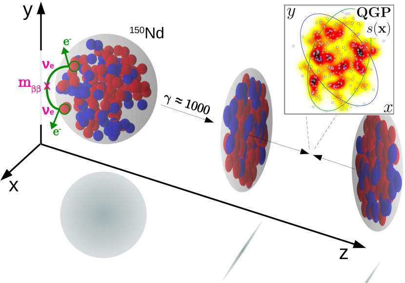
Introduction. The discovery of neutrino oscillations shows that neutrinos are massive particles [1, 2, 3], providing a compelling case for the search of decay, a hypothetical nuclear transition [4] in which two neutrons decay into two protons with the emission of two electrons, but no (anti)neutrinos. Its observation would allow us to determine the nature of the neutrino (Dirac or Majorana) [5], and would demonstrate the violation of the lepton number in nature, shedding light on the origin of the matter-antimatter asymmetry [6]. Furthermore, if this process is driven by the standard mechanism of light Majorana neutrino exchange (left of Fig. 1), the half-life of decay could give insights into the absolute neutrino masses and their hierarchy. Having a good theoretical control of the NME of the transition, which links experimental signals to the effective neutrino mass, is crucial for the design and interpretation of current and future ton-scale experiments [7].
Obtaining a knowledge of the NME that is both accurate and consistent across models poses a major challenge for nuclear theory. The values predicted by different models vary by factors of three or more, leading to an uncertainty of an order of magnitude in the half-life for a given effective neutrino mass [8, 9, 7]. Despite significant progress in calculating the NMEs of candidate nuclei from first principles [10, 11, 12, 13], the uncertainty dominated by many-body truncations remains substantial [14]. To mitigate this problem, considerable effort has been devoted to exploring correlations between the NMEs and experimental observables from low-energy nuclear structure experiments, such as double Gamow-Teller transitions [15, 16, 17, 18] and double-gamma transitions [19, 20]. Notably, correlations between the NMEs and the low-lying states of the candidate nuclei have been examined using a Bayesian analysis within the interacting shell models [21, 22], the valence-space in-medium similarity renormalization group [23], as well as the multi-reference covariant density functional theory (MR-CDFT) [24, 25]. These studies have revealed strong correlations between the NMEs, the excitation energies of the first states, and the values of the candidates. These findings corroborate the observation that the NMEs are sensitive to the deformation parameters of the candidate isotopes [26, 27, 14, 28].
At the other end of the energy spectrum, collider studies have established that measurements of the collective flow of hadrons in the soft sector of high-energy nuclear collisions enable us to experimentally access fine properties of the shapes and radial distributions of nuclei in their ground states [29, 30, 31, 32, 33, 34, 35, 36, 37]. In particular, by studying how observables such as anisotropic flow coefficients vary across collision systems involving isobaric isotopes [38], one can measure signatures of the structure of these nuclei while drastically mitigating the impact of theoretical uncertainties on poorly understood features of the QGP, such as out-of-equilibrium or hadronization phenomena, in the interpretation of the data [39, 40, 41, 42, 43, 44, 45, 46, 47]. Therefore, collider experiments with isobars provide robust probes of the nuclear geometry, and since decay is expected to occur between two isobaric ground states, it is natural to leverage this new knowledge to assess how high-energy experiments constrain model determinations of the NME.
In this Letter, we take a first step in this direction. We couple the aforementioned MR-CDFT-based Bayesian analysis [24, 25] to state-of-the-art simulations of high-energy nuclear collisions, and study the correlation between the NME of the 150Nd150Sm transition and geometric properties of the QGP that are experimentally accessible via collective flow measurements. The signal we find is as strong as that obtained by correlating the NME with more traditional electromagnetic probes of the nuclear geometry. We demonstrate, thus, an experimental technique for the benchmark of NME calculations that is complementary to low-energy nuclear physics methods.
NME, nuclear structure, and heavy-ion collisions. The NME of decay for the transition from the ground state () of \nuclide[150]Nd to the ground state () of \nuclide[150]Sm is given by
| (1) |
where is the transition operator based on the standard mechanism of exchange of light Majorana neutrinos.
The decay operator receives contributions from vector coupling (VV), axial-vector coupling (AA), interference of axial-vector and induced pseudoscalar coupling (AP), induced pseudoscalar coupling (PP), and weak-magnetism coupling (MM) terms, which are related to the products of two current operators [48, 27]. We note that the contact transition operator [49] and two-body currents are not included, as it has been shown that, within the relativistic framework, the renormalizability of the transition amplitude is automatically ensured at leading order [50], rendering the contact transition operator a subleading contribution.
The ground-state wave functions, , of the candidates are determined within the MR-CDFT approach. As detailed in the Supplemental Material (SM), the wave functions are constructed as linear combinations of particle-number (, ), and angular-momentum () projected mean-field wave functions, , with collective coordinate ,
| (2) |
where is a weight, and are projection operators. The states are determined through a deformation-constrained relativistic mean-field (RMF) model coupled to Bardeen–Cooper–Schrieffer (BCS) theory [51, 52]. For the nuclear Hamiltonian, we employ a relativistic energy density functional (EDF) composed of the kinetic energy, , the electromagnetic energy, , as well as the nucleon-nucleon () interaction energy [51, 52, 25],
| (3) |
where and encode different types of densities and currents, and their derivatives. The interaction energy, , is parameterized as a function of via parameters collectively denoted by . The subscripts indicate the scalar and vector types of interaction vertices in Minkowski space, respectively, while subscript is for the vector type in isospin space [52].
Subsequently, the ground-state wave functions obtained from Eq. (2) are used to initialize simulations of high-energy 150Nd+150Nd collisions. With knowledge of the first and states, we compute the electric quadrupole transition strength . As both \nuclide[150]Nd and \nuclide[150]Sm are well-deformed nuclei [53], it is reasonable to relate the quadrupole deformation parameter, , of the intrinsic proton density to the square root of [54]:
| (4) |
where fm. Due to the ultra-short time scales involved, a heavy-ion collision at high energy is understood to take a snapshot of the positions of the nucleons as sampled from the nuclear intrinsic shape with a random orientation in space (right of Fig. 1). Following previous studies [55, 56, 57, 44], the relevant intrinsic density in three-dimensional space, , is determined through a RMF+BCS calculation, denoted single-reference (SR)-CDFT, with a constraint on the mass quadrupole deformation parameter, . Using with the constrained as input, we simulate 150Nd+150Nd collisions at ultrarelativistic energy.
The simulations follow the TENTo model of initial conditions [58], whose working principles are recalled in the SM. The output of the collisions is the entropy density of the QGP in the transverse plane, , one example of which is shown in Fig. 1. To relate this density to experimental observables, two quantities are used:
| (5) |
where . The first quantity, , is the dimensionless spatial ellipticity of the QGP [59], strongly sensitive to the quadrupole deformation of the colliding nuclei [60]. The quantity is proportional to the ratio of the total energy of the QGP to its total entropy. The energy density, , is obtained by applying the QCD equation of state. In particular, at the initial condition of heavy-ion collisions the temperature of the QGP is high enough to justify a simple ideal gas prescription, namely, , with . The total energy is determined, thus, by the steepness of the spatial gradients of the entropy density. As determines the amount of final-state hadrons, is proportional to the energy per particle.
We simulate 106 collisions (or events) at zero impact parameter (ultra-central collisions), which present a strong sensitivity to nuclear deformations. From the ensemble of and values, we evaluate the following averages:
| (6) |
with , which give access to final-state observable quantities, as we explain in the next section.
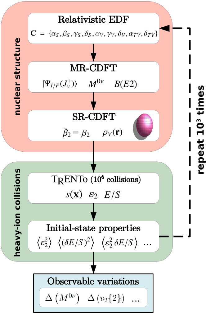
Our workflow is summarized in Fig. 2. We start by generating a set, , of parameters of the nuclear EDF. From that, we evaluate the NME, , as well as an intrinsic nuclear shape with quadrupole deformation, , determined from the transition strength . The intrinsic nuclear shape is used to simulate 106 ultra-central 150Nd+150Nd collisions. We obtain thus a distribution of and values, from which we evaluate the averages in Eq. (6). The process is repeated for 103 samplings of EDF parameters. We stress that for each choice of the initial , the results of the subsequent CDFT calculation represent equally good descriptions of the structure of 150Nd, as they come from a Bayesian analysis of nuclear structure data [25]. This means that any spread in results for the quantities in Eq. (6) should be understood as a systematic theoretical uncertainty due to the imperfect knowledge of nuclear deformation in a model fitted to low-energy data.
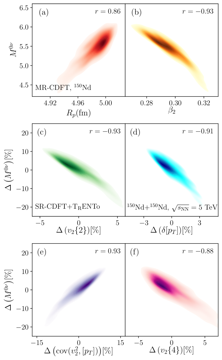
Results and discussion. In Fig. 3(a)-(b), we show how the NME is correlated with the nuclear proton radius, , and the quadrupole deformation parameter, , in the Bayesian analysis. The notable feature is that, while the relative systematic uncertainty on the proton radius is less than 0.5%, the distribution of shows variations up to 10% around the mean value. This implies that fitting observables such as does not lead to a precise knowledge of the detailed many-body properties of the ground state. As a consequence, the NME also shows a relative systematic uncertainty larger than 10%.
We now move on to discuss correlations between the NME and observable features of the QGP produced in 150Nd+150Nd collisions. We recall that signatures of nuclear structure are mainly observed in the distribution of the soft hadrons emitted to the final states [61]. Their spectrum in a class of events (e.g., ultra-central collisions) in the transverse plane at (following, e.g., Fig. 1) is measured differentially in transverse momentum, . Its angular distribution is decomposed in modes [62]:
| (7) |
In what follows we shall need the second harmonic, , which quantifies the elliptic flow of the system, as well as the average hadron momentum, .
Hydrodynamic simulations indicate that the final-state elliptic flow coefficient, , is in a strong linear correlation with the initial-state ellipticity parameter, [63, 64, 65]. Similarly, the average transverse momentum (which measures the energy per particle) is correlated with the value of [66, 67]. For an observable , we define its relative variation by:
| (8) |
where the subscript denotes an average over samples of the EDF parameter set. We consider, then, the variation of the following observables, where the pre-factors ensure that they can be meaningfully compared to each other:
| (9) |
The proportionality factors in the relations and cancel out in the definition of . Therefore, the variations of the final-state observables in Eq. (Benchmarking nuclear matrix elements of decay with high-energy nuclear collisions) can be estimated from the variations of the initial-state quantities in Eq. (6).
.
Our results are in Fig.3(c)-(f) for ultra-central 150Nd+150Nd collisions. We see that driven by the change in quadrupole deformation, both and the fluctuation [panel (c) and (d)] vary by several percent, in agreement with recent hydrodynamic studies [68, 69]. A similar variation is observed for the cumulant [panel (f)], as nuclear deformation enhances the non-Gaussianity (kurtosis) of the distribution of the elliptic flow vector [29, 70, 71]. Finally, the covariance of and in Fig. 3(e) presents the strongest variation, changing by about 10%, with a positive correlation due to the fact that and are anti-correlated in the presence of a large [72, 73, 74, 75, 68, 69, 36].
Our main result is that all of these variations are strongly correlated with the value of the NME. The question, then, is whether the spread in NME values would be reduced if the nuclear model were constrained to ensure a precise description of the collective flow measurements following high-energy collision simulations. For this to be the case, the addition of high-energy data to the Bayesian analysis should effectively improve the extraction of the nuclear deformation, without introducing any substantial systematic uncertainties. We reiterate, then, that by combining flow observables among different collision systems of similar size (as done recently for 96Ru+96Ru vs. 96Zr+96Zr, or 197Au+197Au vs. 238U+238U), it is possible to isolate signatures of the geometry of the colliding isotopes while suppressing the impact of the uncertainty on our knowledge of the QGP, such as the detailed values of its transport coefficient in hydrodynamics [39, 40, 36, 47]. For example, taking the well-known near-spherical nucleus 208Pb as a baseline, the hydrodynamic studies suggest that a ratio of observables of the type: , will depend almost exclusively on the differences in structure between 150Nd and 208Pb. Therefore, we expect that a combined Bayesian analysis of low-energy nuclear structure data and high-energy heavy-ion data will lead to an improved determination of . As a consequence, the uncertainty on the NME will decrease.
Summary and outlook. The results of a Bayesian analysis of low-energy nuclear structure data in the framework of CDFT are coupled to simulations of high-energy collisions, highlighting the existence of strong correlations between the value of the NME of decay and quantities accessible at colliders. Our conclusion is that it is possible to leverage measurements of the observables discussed in Fig. 3 to benchmark theoretical predictions of the NME.
This result has to be followed up by a combined Bayesian analysis of low- and high-energy data (likely by means of mock experimental data in the absence of collider results on the candidate isotopes), which would yield a better handle on the nuclear deformation and thus on the NME. In doing so, one should also include the octupole and the triaxial deformation of the candidate isotopes, which are expected to impact the values of the matrix elements, and which can be targeted by observables such as , the triangular flow, , or the skewness of fluctuations [55, 76, 75, 77]. Moreover, it should be investigated whether combining data sets from 150Nd+150Nd and 150Sm+150Sm collisions (or other pairs of candidates) gives access to relative observables that may present an even tighter correlation with the NME.
We note that, from a high-energy experiment point of view, it is rather straightforward to collect a statistics of ultra-central events sufficient to measure observables including with a relative uncertainty of 1% or less, which seems required from the plots shown in Fig. 3. At the Large Hadron Collider (LHC), and thanks to upcoming detector upgrades such as ALICE 3 [78], such results could be obtained via short special collision runs of only a few hours. The potential upgrade of the ion injector complex with the addition of a second ion source [79] will enable us, furthermore, to collide ions in the aforementioned isobar operation mode, which will reduce experimental and theoretical systematic uncertainties on the flow measurements, isolating clean signals of the nuclear geometries. Therefore, a potential spin-off of the LHC ion program connecting with the next generation of decay searches appears technically within reach and worth pursuing.
Acknowledgements.
Acknowledgments. We thank Lotta Jokiniemi, Huichao Song, as well as the participants of the CERN workshop “Nuclear Shape and BSM Searches at Colliders” for useful discussions. This work was supported in part by the National Natural Science Foundation of China (Grant Nos. 12375119 and 12141501), and the Guangdong Basic and Applied Basic Research Foundation (2023A1515010936).I Supplemental material
MR-CDFT framework.
The wave function of nuclear low-lying state is constructed as a superposition of quantum-number projected mean-field wave functions [80],
| (10) |
where distinguishes different states with the same quantum numbers , while is the number of deformed projected basis functions which are constructed as
| (11) |
The weight function is determined by solving the Hill-Wheeler-Griffin equation [81, 80],
| (12) |
The intrinsic mean-field states are obtained by minimizing the EDF with respect to the single-particle wave function , which leads to Dirac equation
| (13) |
where is the mass of the nucleon, while the scalar and vector potentials, respectively and , are functions of densities and currents [52].
The total number density of an atomic nucleus, corresponding to the time-like component of the four-component current, is given by the sum of the densities of each nucleon,
| (14) |
where is the occupation probability of the -th single-particle state, and its value is determined by BCS theory based on a zero-range pairing force. The wave function , corresponding to collective coordinate , is approximated by a BCS wave function. The intrinsic shape of the nucleus is characterized with dimensionless multipole moments,
| (15) |
with fm. The value of is in particular matched to the value of obtained using Eq. (4). The transition strength is also determined in the full MR-CDFT framework. With the weight functions for the initial and final states, the electric quadrupole () transition strength for can be computed by
where is the bare electric quadrupole moment operator. More details about the MR-CDFT, its emulator, and the sampling of parameter sets for the relativistic EDF can be found in Ref. [25].
Collision simulations and observables.
The particle density in Eq. (14) is utilized as input for performing high-energy 150Nd+150Nd collisions. For completeness, we report here a brief summary of the TENTo model employed in these simulations. The same model setup has been described in greater detail in previous publications, see e.g. [55].
The coordinates of nucleons are sampled for each of the colliding ions using as a particle density. We generate a random orientation for both colliding nuclei (six Euler angles in total), and then rotate the coordinates of the sampled nucleons accordingly. These coordinates are eventually shifted by an impact parameter in the transverse plane, , which we can take along the direction without any loss of generality. Inter-nucleon distances among nucleons coming from different nuclei are evaluated, and a given nucleon in nucleus is flagged as a participant if it lies within a radius from another nucleon belonging to nucleus , or vice versa. We take fm2 to simulate collisions at top LHC energy, TeV.
The thickness functions of the nuclei, respectively, and , are given by a superposition of nucleonic profiles:
| (17) |
Here is the coordinate in the plane transverse to the beam direction ( direction), while is the location of the th participant nucleon inside nucleus (which has a total of participants). Each nucleon is associated with a Gaussian profile of width fm, and a random normalization, , sampled from a gamma distribution of unit mean and variance, , with , a choice consistent with a previous Bayesian analysis of LHC data [82].
From the thickness functions we construct the entropy of the initial state, , following the Ansatz:
| (18) |
strongly supported by phenomenological applications. Next, we compute the th order spatial anisotropy, , and the energy over the entropy of the system, , as discussed in the text. For each initial we simulate 106 collisions, and then calculate the event averages that lead to the observable quantities shown in Fig. 3 for collisions at .
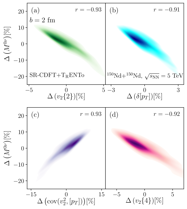
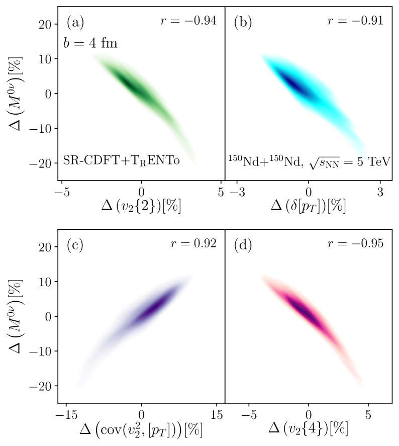
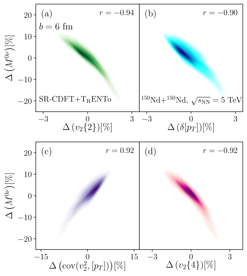
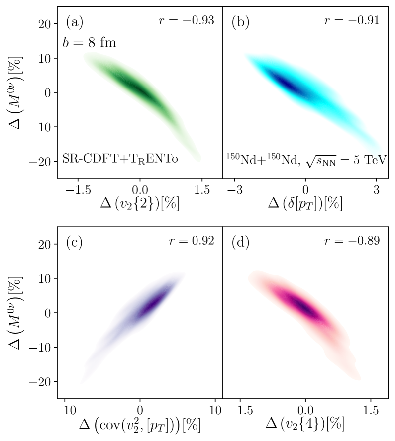
For completeness, Figs. 4, 5, 6, 7 present results for higher values of the impact parameter of the collisions. The strong correlations between the observables and the NME persist up to large impact parameters. However, one can note that the relative variations in terms of percentage are much reduced at the highest values of , consistent with the fact that the nuclear deformations impact mostly central collisions that fully resolve the geometry of the colliding bodies.
References
- Ahmad et al. [2001] Q. R. Ahmad et al. (SNO), Measurement of the rate of interactions produced by 8B solar neutrinos at the Sudbury Neutrino Observatory, Phys. Rev. Lett. 87, 071301 (2001), arXiv:nucl-ex/0106015 .
- Eguchi et al. [2003] K. Eguchi et al. (KamLAND), First results from KamLAND: Evidence for reactor anti-neutrino disappearance, Phys. Rev. Lett. 90, 021802 (2003), arXiv:hep-ex/0212021 .
- An et al. [2012] F. P. An et al. (Daya Bay), Observation of electron-antineutrino disappearance at Daya Bay, Phys. Rev. Lett. 108, 171803 (2012), arXiv:1203.1669 [hep-ex] .
- Furry [1939] W. H. Furry, On transition probabilities in double beta-disintegration, Phys. Rev. 56, 1184 (1939).
- Schechter and Valle [1982] J. Schechter and J. W. F. Valle, Neutrinoless Double beta Decay in SU(2) x U(1) Theories, Phys. Rev. D 25, 2951 (1982).
- Fukugita and Yanagida [1986] M. Fukugita and T. Yanagida, Baryogenesis Without Grand Unification, Phys. Lett. B 174, 45 (1986).
- Agostini et al. [2023] M. Agostini, G. Benato, J. A. Detwiler, J. Menéndez, and F. Vissani, Toward the discovery of matter creation with neutrinoless decay, Rev. Mod. Phys. 95, 025002 (2023), arXiv:2202.01787 [hep-ex] .
- Engel and Menéndez [2017] J. Engel and J. Menéndez, Status and Future of Nuclear Matrix Elements for Neutrinoless Double-Beta Decay: A Review, Rept. Prog. Phys. 80, 046301 (2017), arXiv:1610.06548 [nucl-th] .
- Yao et al. [2022a] J. M. Yao, J. Meng, Y. F. Niu, and P. Ring, Beyond-mean-field approaches for nuclear neutrinoless double beta decay in the standard mechanism, Prog. Part. Nucl. Phys. 126, 103965 (2022a), arXiv:2111.15543 [nucl-th] .
- Yao et al. [2020] J. M. Yao, B. Bally, J. Engel, R. Wirth, T. R. Rodríguez, and H. Hergert, Ab initio treatment of collective correlations and the neutrinoless double beta decay of , Phys. Rev. Lett. 124, 232501 (2020).
- Belley et al. [2021] A. Belley, C. G. Payne, S. R. Stroberg, T. Miyagi, and J. D. Holt, Neutrinoless Double-Beta Decay Matrix Elements for 48Ca , 76Ge , and 82Se, Phys. Rev. Lett. 126, 042502 (2021), arXiv:2008.06588 [nucl-th] .
- Novario et al. [2021] S. Novario, P. Gysbers, J. Engel, G. Hagen, G. R. Jansen, T. D. Morris, P. Navrátil, T. Papenbrock, and S. Quaglioni, Coupled-Cluster Calculations of Neutrinoless Double- Decay in 48Ca, Phys. Rev. Lett. 126, 182502 (2021), arXiv:2008.09696 [nucl-th] .
- Belley et al. [2024a] A. Belley, J. Pitcher, T. Miyagi, S. R. Stroberg, and J. D. Holt, Correlation of neutrinoless double-beta decay nuclear matrix elements with nucleon-nucleon phase shifts, (2024a), arXiv:2408.02169 [nucl-th] .
- Belley et al. [2024b] A. Belley, J. M. Yao, B. Bally, J. Pitcher, J. Engel, H. Hergert, J. D. Holt, T. Miyagi, T. R. Rodríguez, A. M. Romero, S. R. Stroberg, and X. Zhang, Ab initio uncertainty quantification of neutrinoless double-beta decay in , Phys. Rev. Lett. 132, 182502 (2024b).
- Shimizu et al. [2018] N. Shimizu, J. Menéndez, and K. Yako, Double Gamow-Teller Transitions and its Relation to Neutrinoless Decay, Phys. Rev. Lett. 120, 142502 (2018), arXiv:1709.01088 [nucl-th] .
- Yao et al. [2022b] J. M. Yao, I. Ginnett, A. Belley, T. Miyagi, R. Wirth, S. Bogner, J. Engel, H. Hergert, J. D. Holt, and S. R. Stroberg, Ab initio studies of the double–Gamow-Teller transition and its correlation with neutrinoless double- decay, Phys. Rev. C 106, 014315 (2022b), arXiv:2204.12971 [nucl-th] .
- Jokiniemi and Menéndez [2023] L. Jokiniemi and J. Menéndez, Correlations between neutrinoless double-, double Gamow-Teller, and double-magnetic decays in the proton-neutron quasiparticle random-phase approximation framework, Phys. Rev. C 107, 044316 (2023), arXiv:2302.05399 [nucl-th] .
- Wang et al. [2024] Y. K. Wang, P. W. Zhao, and J. Meng, Correlation between neutrinoless double- decay and double Gamow-Teller transitions, Phys. Lett. B 855, 138796 (2024), arXiv:2403.06455 [nucl-th] .
- Romeo et al. [2022] B. Romeo, J. Menéndez, and C. Peña Garay, decay as a probe of neutrinoless decay nuclear matrix elements, Phys. Lett. B 827, 136965 (2022), arXiv:2102.11101 [nucl-th] .
- Romeo et al. [2025] B. Romeo, D. Stramaccioni, J. Menéndez, and J. J. Valiente-Dobón, A pathway to unveiling neutrinoless decay nuclear matrix elements via decay, Phys. Lett. B 860, 139186 (2025), arXiv:2411.03539 [nucl-th] .
- Horoi et al. [2022] M. Horoi, A. Neacsu, and S. Stoica, Statistical analysis for the neutrinoless double--decay matrix element of Ca48, Phys. Rev. C 106, 054302 (2022), arXiv:2203.10577 [nucl-th] .
- Horoi et al. [2023] M. Horoi, A. Neacsu, and S. Stoica, Predicting the neutrinoless double--decay matrix element of Xe136 using a statistical approach, Phys. Rev. C 107, 045501 (2023), arXiv:2302.03664 [nucl-th] .
- Belley et al. [2022] A. Belley, T. Miyagi, S. R. Stroberg, and J. D. Holt, Constraining Neutrinoless Double-Beta Decay Matrix Elements from Ab Initio Nuclear Theory, in Matrix Elements for the Double-beta-decay EXperiments (2022) arXiv:2210.05809 [nucl-th] .
- Zhang et al. [2024a] X. Zhang, C. C. Wang, C. R. Ding, and J. M. Yao, Subspace-projected multireference covariant density functional theory, (2024a), arXiv:2408.00691 [nucl-th] .
- Zhang et al. [2024b] X. Zhang, C. C. Wang, C. R. Ding, and J. M. Yao, Global sensitivity analysis and uncertainty quantification of nuclear low-lying states and double-beta decay with a covariant energy density functional, (2024b), arXiv:2408.13209 [nucl-th] .
- Rodríguez and Martínez-Pinedo [2010] T. R. Rodríguez and G. Martínez-Pinedo, Energy density functional study of nuclear matrix elements for neutrinoless decay, Phys. Rev. Lett. 105, 252503 (2010).
- Yao et al. [2015a] J. M. Yao, L. S. Song, K. Hagino, P. Ring, and J. Meng, Systematic study of nuclear matrix elements in neutrinoless double- decay with a beyond-mean-field covariant density functional theory, Phys. Rev. C 91, 024316 (2015a).
- Jiao et al. [2023] C. Jiao, C. Yuan, and J. Yao, Correlation of Neutrinoless Double- Decay Nuclear Matrix Element with E2 Strength, Symmetry 15, 552 (2023).
- Adamczyk et al. [2015] L. Adamczyk et al. (STAR), Azimuthal anisotropy in UU and AuAu collisions at RHIC, Phys. Rev. Lett. 115, 222301 (2015), arXiv:1505.07812 [nucl-ex] .
- Acharya et al. [2018] S. Acharya et al. (ALICE), Anisotropic flow in Xe-Xe collisions at TeV, Phys. Lett. B 784, 82 (2018), arXiv:1805.01832 [nucl-ex] .
- Sirunyan et al. [2019] A. M. Sirunyan et al. (CMS), Charged-particle angular correlations in XeXe collisions at 5.44 TeV, Phys. Rev. C 100, 044902 (2019), arXiv:1901.07997 [hep-ex] .
- Aad et al. [2020] G. Aad et al. (ATLAS), Measurement of the azimuthal anisotropy of charged-particle production in collisions at TeV with the ATLAS detector, Phys. Rev. C 101, 024906 (2020), arXiv:1911.04812 [nucl-ex] .
- Abdallah et al. [2022] M. Abdallah et al. (STAR), Search for the chiral magnetic effect with isobar collisions at =200 GeV by the STAR Collaboration at the BNL Relativistic Heavy Ion Collider, Phys. Rev. C 105, 014901 (2022), arXiv:2109.00131 [nucl-ex] .
- Acharya et al. [2022] S. Acharya et al. (ALICE), Characterizing the initial conditions of heavy-ion collisions at the LHC with mean transverse momentum and anisotropic flow correlations, Phys. Lett. B 834, 137393 (2022), arXiv:2111.06106 [nucl-ex] .
- Aad et al. [2023] G. Aad et al. (ATLAS), Correlations between flow and transverse momentum in Xe+Xe and Pb+Pb collisions at the LHC with the ATLAS detector: A probe of the heavy-ion initial state and nuclear deformation, Phys. Rev. C 107, 054910 (2023), arXiv:2205.00039 [nucl-ex] .
- Abdulhamid et al. [2024] M. I. Abdulhamid et al. (STAR), Imaging shapes of atomic nuclei in high-energy nuclear collisions, Nature 635, 67 (2024), arXiv:2401.06625 [nucl-ex] .
- Acharya et al. [2024] S. Acharya et al. (ALICE), Exploring nuclear structure with multiparticle azimuthal correlations at the LHC, (2024), arXiv:2409.04343 [nucl-ex] .
- Giacalone et al. [2021a] G. Giacalone, J. Jia, and V. Somà, Accessing the shape of atomic nuclei with relativistic collisions of isobars, Phys. Rev. C 104, L041903 (2021a), arXiv:2102.08158 [nucl-th] .
- Xu et al. [2023] H.-j. Xu, W. Zhao, H. Li, Y. Zhou, L.-W. Chen, and F. Wang, Probing nuclear structure with mean transverse momentum in relativistic isobar collisions, Phys. Rev. C 108, L011902 (2023), arXiv:2111.14812 [nucl-th] .
- Nijs and van der Schee [2023] G. Nijs and W. van der Schee, Inferring nuclear structure from heavy isobar collisions using Trajectum, SciPost Phys. 15, 041 (2023), arXiv:2112.13771 [nucl-th] .
- Zhang et al. [2022] C. Zhang, S. Bhatta, and J. Jia, Ratios of collective flow observables in high-energy isobar collisions are insensitive to final-state interactions, Phys. Rev. C 106, L031901 (2022), arXiv:2206.01943 [nucl-th] .
- Zhao et al. [2023] S. Zhao, H.-j. Xu, Y.-X. Liu, and H. Song, Probing the nuclear deformation with three-particle asymmetric cumulant in RHIC isobar runs, Phys. Lett. B 839, 137838 (2023), arXiv:2204.02387 [nucl-th] .
- Gardim et al. [2024] F. G. Gardim, A. V. Giannini, F. Grassi, K. P. Pala, and W. M. Serenone, Impact of the pre-equilibrium stage for the determination of nuclear geometry in high-energy isobar collisions, Phys. Rev. C 110, 064907 (2024), arXiv:2305.03703 [nucl-th] .
- Giacalone et al. [2024a] G. Giacalone et al., The unexpected uses of a bowling pin: exploiting 20Ne isotopes for precision characterizations of collectivity in small systems, (2024a), arXiv:2402.05995 [nucl-th] .
- Giacalone et al. [2024b] G. Giacalone et al., The unexpected uses of a bowling pin: anisotropic flow in fixed-target 208Pb+20Ne collisions as a probe of quark-gluon plasma, (2024b), arXiv:2405.20210 [nucl-th] .
- Xu et al. [2024] H.-j. Xu, J. Zhao, and F. Wang, Hexadecapole Deformation of U238 from Relativistic Heavy-Ion Collisions Using a Nonlinear Response Coefficient, Phys. Rev. Lett. 132, 262301 (2024), arXiv:2402.16550 [nucl-th] .
- Mäntysaari et al. [2024] H. Mäntysaari, B. Schenke, C. Shen, and W. Zhao, Probing nuclear structure of heavy ions at energies available at the CERN Large Hadron Collider, Phys. Rev. C 110, 054913 (2024), arXiv:2409.19064 [nucl-th] .
- Song et al. [2014] L. S. Song, J. M. Yao, P. Ring, and J. Meng, Relativistic description of nuclear matrix elements in neutrinoless double- decay, Phys. Rev. C 90, 054309 (2014).
- Cirigliano et al. [2018] V. Cirigliano, W. Dekens, J. de Vries, M. L. Graesser, E. Mereghetti, S. Pastore, and U. van Kolck, New leading contribution to neutrinoless double- decay, Phys. Rev. Lett. 120, 202001 (2018).
- Yang and Zhao [2024] Y. Yang and P. Zhao, Relativistic model-free prediction for neutrinoless double beta decay at leading order, Physics Letters B 855, 138782 (2024).
- Burvenich et al. [2002] T. Burvenich, D. G. Madland, J. A. Maruhn, and P. G. Reinhard, Nuclear ground state observables and QCD scaling in a refined relativistic point coupling model, Phys. Rev. C 65, 044308 (2002), arXiv:nucl-th/0111012 .
- Zhao et al. [2010] P. W. Zhao, Z. P. Li, J. M. Yao, and J. Meng, New parametrization for the nuclear covariant energy density functional with point-coupling interaction, Phys. Rev. C 82, 054319 (2010), arXiv:1002.1789 [nucl-th] .
- Yao et al. [2015b] J. M. Yao, L. S. Song, K. Hagino, P. Ring, and J. Meng, Systematic study of nuclear matrix elements in neutrinoless double- decay with a beyond-mean-field covariant density functional theory, Phys. Rev. C 91, 024316 (2015b), arXiv:1410.6326 [nucl-th] .
- Raman et al. [2001] S. Raman, C. Nestor, and P. Tikkanen, Transition probability from the ground to the first-excited 2+ state of even–even nuclides, Atomic Data and Nuclear Data Tables 78, 1 (2001).
- Bally et al. [2022] B. Bally, M. Bender, G. Giacalone, and V. Somà, Evidence of the triaxial structure of 129Xe at the Large Hadron Collider, Phys. Rev. Lett. 128, 082301 (2022), arXiv:2108.09578 [nucl-th] .
- Bally et al. [2023] B. Bally, G. Giacalone, and M. Bender, The shape of gold, Eur. Phys. J. A 59, 58 (2023), arXiv:2301.02420 [nucl-th] .
- Ryssens et al. [2023] W. Ryssens, G. Giacalone, B. Schenke, and C. Shen, Evidence of Hexadecapole Deformation in Uranium-238 at the Relativistic Heavy Ion Collider, Phys. Rev. Lett. 130, 212302 (2023), arXiv:2302.13617 [nucl-th] .
- Moreland et al. [2015] J. S. Moreland, J. E. Bernhard, and S. A. Bass, Alternative ansatz to wounded nucleon and binary collision scaling in high-energy nuclear collisions, Phys. Rev. C 92, 011901 (2015), arXiv:1412.4708 [nucl-th] .
- Teaney and Yan [2011] D. Teaney and L. Yan, Triangularity and Dipole Asymmetry in Heavy Ion Collisions, Phys. Rev. C 83, 064904 (2011), arXiv:1010.1876 [nucl-th] .
- Giacalone et al. [2021b] G. Giacalone, J. Jia, and C. Zhang, Impact of Nuclear Deformation on Relativistic Heavy-Ion Collisions: Assessing Consistency in Nuclear Physics across Energy Scales, Phys. Rev. Lett. 127, 242301 (2021b), arXiv:2105.01638 [nucl-th] .
- Giacalone [2023] G. Giacalone, Many-body correlations for nuclear physics across scales: from nuclei to quark-gluon plasmas to hadron distributions, Eur. Phys. J. A 59, 297 (2023), arXiv:2305.19843 [nucl-th] .
- Ollitrault [2023] J.-Y. Ollitrault, Measures of azimuthal anisotropy in high-energy collisions, Eur. Phys. J. A 59, 236 (2023), arXiv:2308.11674 [nucl-ex] .
- Niemi et al. [2013] H. Niemi, G. S. Denicol, H. Holopainen, and P. Huovinen, Event-by-event distributions of azimuthal asymmetries in ultrarelativistic heavy-ion collisions, Phys. Rev. C 87, 054901 (2013), arXiv:1212.1008 [nucl-th] .
- Noronha-Hostler et al. [2016] J. Noronha-Hostler, L. Yan, F. G. Gardim, and J.-Y. Ollitrault, Linear and cubic response to the initial eccentricity in heavy-ion collisions, Phys. Rev. C 93, 014909 (2016), arXiv:1511.03896 [nucl-th] .
- Sousa et al. [2024] J. Sousa, J. Noronha, and M. Luzum, Initial energy-momentum to final flow: A general framework for heavy-ion collisions, Phys. Rev. C 110, 044909 (2024), arXiv:2405.13600 [nucl-th] .
- Schenke et al. [2020] B. Schenke, C. Shen, and D. Teaney, Transverse momentum fluctuations and their correlation with elliptic flow in nuclear collision, Phys. Rev. C 102, 034905 (2020), arXiv:2004.00690 [nucl-th] .
- Giacalone et al. [2021c] G. Giacalone, F. G. Gardim, J. Noronha-Hostler, and J.-Y. Ollitrault, Correlation between mean transverse momentum and anisotropic flow in heavy-ion collisions, Phys. Rev. C 103, 024909 (2021c), arXiv:2004.01765 [nucl-th] .
- Fortier et al. [2025a] N. M. Fortier, S. Jeon, and C. Gale, Comparisons and predictions for collisions of deformed U238 nuclei at sNN=193 GeV, Phys. Rev. C 111, 014901 (2025a), arXiv:2308.09816 [nucl-th] .
- Fortier et al. [2025b] N. M. Fortier, S. Jeon, and C. Gale, Heavy-ion collisions as probes of nuclear structure, Phys. Rev. C 111, L011901 (2025b), arXiv:2405.17526 [nucl-th] .
- Giacalone [2019] G. Giacalone, Elliptic flow fluctuations in central collisions of spherical and deformed nuclei, Phys. Rev. C 99, 024910 (2019), arXiv:1811.03959 [nucl-th] .
- Mehrabpour and Tabatabaee [2023] H. Mehrabpour and S. M. A. Tabatabaee, Flow distribution analysis as a probe of nuclear deformation, Phys. Rev. C 108, 034902 (2023), arXiv:2301.07770 [nucl-th] .
- Giacalone [2020a] G. Giacalone, Observing the deformation of nuclei with relativistic nuclear collisions, Phys. Rev. Lett. 124, 202301 (2020a), arXiv:1910.04673 [nucl-th] .
- Giacalone [2020b] G. Giacalone, Constraining the quadrupole deformation of atomic nuclei with relativistic nuclear collisions, Phys. Rev. C 102, 024901 (2020b), arXiv:2004.14463 [nucl-th] .
- Jia et al. [2022] J. Jia, S. Huang, and C. Zhang, Probing nuclear quadrupole deformation from correlation of elliptic flow and transverse momentum in heavy ion collisions, Phys. Rev. C 105, 014906 (2022), arXiv:2105.05713 [nucl-th] .
- Jia [2022] J. Jia, Probing triaxial deformation of atomic nuclei in high-energy heavy ion collisions, Phys. Rev. C 105, 044905 (2022), arXiv:2109.00604 [nucl-th] .
- Zhang and Jia [2022] C. Zhang and J. Jia, Evidence of Quadrupole and Octupole Deformations in Zr96+Zr96 and Ru96+Ru96 Collisions at Ultrarelativistic Energies, Phys. Rev. Lett. 128, 022301 (2022), arXiv:2109.01631 [nucl-th] .
- Nielsen et al. [2024] E. G. D. Nielsen, F. K. Rømer, K. Gulbrandsen, and Y. Zhou, Generic multi-particle transverse momentum correlations as a new tool for studying nuclear structure at the energy frontier, Eur. Phys. J. A 60, 38 (2024), arXiv:2312.00492 [nucl-th] .
- ALI [2022] Letter of intent for ALICE 3: A next-generation heavy-ion experiment at the LHC, (2022), arXiv:2211.02491 [physics.ins-det] .
- Alemany Fernandez [2025] R. Alemany Fernandez, Prospects for light-ion operation at the HL-LHC: machine developments and physics opportunities, PoS LHCP2024, 335 (2025).
- Ring and Schuck [1980] P. Ring and P. Schuck, The nuclear many-body problem (Springer-Verlag, New York, 1980).
- Hill and Wheeler [1953] D. L. Hill and J. A. Wheeler, Nuclear constitution and the interpretation of fission phenomena, Phys. Rev. 89, 1102 (1953).
- Bernhard et al. [2016] J. E. Bernhard, J. S. Moreland, S. A. Bass, J. Liu, and U. Heinz, Applying Bayesian parameter estimation to relativistic heavy-ion collisions: simultaneous characterization of the initial state and quark-gluon plasma medium, Phys. Rev. C 94, 024907 (2016), arXiv:1605.03954 [nucl-th] .