Initialization Matters: Unraveling the Impact of Pre-Training on Federated Learning

Abstract

Initializing with pre-trained models when learning on downstream tasks is becoming standard practice in machine learning. Several recent works explore the benefits of pre-trained initialization in a federated learning (FL) setting, where the downstream training is performed at the edge clients with heterogeneous data distribution. These works show that starting from a pre-trained model can substantially reduce the adverse impact of data heterogeneity on the test performance of a model trained in a federated setting, with no changes to the standard FedAvg training algorithm. In this work, we provide a deeper theoretical understanding of this phenomenon. To do so, we study the class of two-layer convolutional neural networks (CNNs) and provide bounds on the training error convergence and test error of such a network trained with FedAvg. We introduce the notion of aligned and misaligned filters at initialization and show that the data heterogeneity only affects learning on misaligned filters. Starting with a pre-trained model typically results in fewer misaligned filters at initialization, thus producing a lower test error even when the model is trained in a federated setting with data heterogeneity. Experiments in synthetic settings and practical FL training on CNNs verify our theoretical findings.

1 Introduction

Federated Learning (FL) (McMahan et al., 2017) has emerged as the de-facto paradigm for training a Machine Learning (ML) model over data distributed across multiple clients with privacy protection due to its no data-sharing philosophy. Ever since its inception, it has been observed that heterogeneity in client data can severely slow down FL training and lead to a model that has poorer generalization performance than a model trained on Independent and Identically Distributed (IID) data (Kairouz et al., 2021; Li et al., 2020; Yang et al., 2021a). This has led works to propose several algorithmic modifications to the popular Federated Averaging (FedAvg) algorithm such as variance-reduction (Acar et al., 2021; Karimireddy et al., 2020), contrastive learning (Li et al., 2021; Tan et al., 2022) and sophisticated model-aggregation techniques (Lin et al., 2020; Wang et al., 2020), to combat the challenge of data heterogeneity.

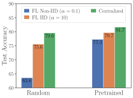
Figure 1: Test accuracy ($\%$) on CIFAR10 with SqueezeNet model (Iandola et al., 2016) under random and pretrained initializations for FL and centralized training. Pre-training benefits FL more than centralized setting and significantly reduces the gap between IID and non-IID FL model performance.

A recent line of work (Chen et al., 2022; Nguyen et al., 2022) has sought to understand the benefits of starting from pre-trained models instead of randomly initializing the global model when doing FL. This idea has been popularized by results in the centralized setting (Devlin et al., 2019; Radford et al., 2019; He et al., 2019; Dosovitskiy et al., 2021), which show that starting from a pre-trained model can lead to state-of-the-art accuracy and faster convergence on downstream tasks. Pre-training is usually done on internet-scale public data (Schuhmann et al., 2022; Thomee et al., 2016; Raffel et al., 2020; Gao et al., 2020) in order for the model to learn fundamental data representations (Sun et al., 2017; Mahajan et al., 2018; Radford et al., 2019), that can be easily applied for downstream tasks. Thus, while it would not be unexpected to see some gains of using pre-trained models even in FL, what is surprising is the sheer scale of improvement. In many cases (Nguyen et al., 2022; Chen et al., 2022) show that just starting from a pre-trained model can significantly reduce the gap between the performance of a model trained in a federated setting with non-IID versus IID data partitioning with no algorithmic modifications. Figure˜1 shows our own replication of this phenomenon, where starting from a pre-trained model can lead to almost $14\%$ improvement in accuracy for FL with non-IID data (i.e., high data heterogeneity) compared to $4\%$ for FL with IID data and $2\%$ in the centralized setting. This observation leads us to ask the question:

Why can pre-trained initialization drastically improve model performance in FL?

One reason suggested by (Nguyen et al., 2022) is a lower value of the training loss at initialization when starting from pre-trained models. However, this observation can only explain improvement in training convergence speed (see Theorem V in (Karimireddy et al., 2021)) and not the significantly improved generalization performance of the trained model. Also, a pre-trained initialization can have larger loss than random initialization while continuing to have faster convergence and better generalization (see Table 1 in (Nguyen et al., 2022)). Chen et al. (2022); Nguyen et al. (2022), also observe some optimization-related factors when starting from a pre-trained model including smaller distance to optimum, better conditioned loss surface (smaller value of the largest eigen value of Hessian) and more stable global aggregation. However, it has not been formally proven that these factors can reduce the adverse effect of non-IID data. Thus, there is still a lack of fundamental understanding of why pre-trained initialization benefits generalization for non-IID FL.

Our contributions. In this work we provide a deeper theoretical understanding of the importance of initialization for FedAvg by studying two-layer ReLU Convolutional Neural Networks (CNNs) for binary classification. This class of neural networks lends itself to tractable analysis while providing valuable insights that extend to training deeper CNNs as shown by several recent works (Cao et al., 2022; Du et al., 2018; Kou et al., 2023; Zou et al., 2023; Jelassi & Li, 2022; Bao et al., 2024; Oh & Yun, 2024). Our data generation model, also studied in (Cao et al., 2022; Kou et al., 2023), allows us to utilize a signal-noise decomposition result (see Proposition˜1) to perform a fine-grained analysis of the CNN filter weight updates than can be done with general non-convex optimization. Some highlights of our results are as follows:

1. We introduce the notion of aligned and misaligned filters at initialization (Lemma˜1) and show that data heterogeneity affects signal learning only on misaligned filters while noise memorization is unaffected by data heterogeneity (see Lemma˜2). A pre-trained model is expected to have fewer misaligned filters, which can explain the reduced effect of non-IID data.

2. We provide a test error upper bound for FedAvg that depends on the number of misaligned filters at initialization and data heterogeneity. The effect of data heterogeneity on misaligned filters is exacerbated as clients perform more local steps, which explains why FL benefits more from pre-trained initialization than centralized training. To our knowledge, this is the first result where the test error for FedAvg explicitly depends on initialization conditions (Theorem˜2).

3. We prove the training error convergence of FedAvg by adopting a two-stage analysis: a first stage where the local loss derivatives are lower bounded by a constant and second stage where the model is in the neighborhood of a global minimizer with nearly convex loss landscape. Our analysis shows a provable benefit of using local steps in the first stage to reduce communication cost.

4. We experimentally verify our upper bound on the test error in a synthetic data setting (see Section˜3 as well as conduct experiments on practical FL tasks which show that our insights extend to deeper CNNs (see Section˜4).

Related Work. The two-layer CNN model that we study in this work was originally introduced in (Zou et al., 2023) for the purpose of analyzing the generalization error of the Adam optimizer in the centralized setting. Later (Cao et al., 2022) study the same model to analyze the phenomenon of benign overfitting in two-layer CNN, i.e., give precise conditions under which the CNN can perfectly fit the data while also achieving small population loss. (Oh & Yun, 2024) use this model to prove the benefit of patch-level data augmentation techniques such as Cutout and CutMix. (Kou et al., 2023) relaxes the the polynomial ReLU activation in (Cao et al., 2022) to the standard ReLU activation and also introduces label-flipping noise when analyzing benign overfitting in the centralized setting. We do not consider label-flipping in our work for simplicity; however this can be easily incorporated as future work. To the best of our knowledge, we are only aware of two other works (Huang et al., 2023; Bao et al., 2024) that analyze the two-layer CNN in a FL setting. The focus in (Huang et al., 2023) is on showing the benefit of collaboration in FL by considering signal heterogeneity across the data in clients while (Bao et al., 2024) considers signal heterogeneity to show the benefit of local steps. Both (Huang et al., 2023) and (Bao et al., 2024) do not consider any label heterogeneity and there is no emphasis on the importance of initialization, making their analysis quite different from ours. We defer more discussion on other related works to the Appendix.

2 Problem Setup

We begin by introducing the data generation model and the two-layer convolutional neural network, followed by our FL objective and a brief primer on the FedAvg algorithm. We note that given integers $a,b$, we denote by $[a:b]$ the set of integers $\{a,a+1,\dots,b\}$. Also, $[n]$ denotes $\{1,2,\dots,n\}$.

Data-Generation Model.

Let $\mathcal{D}$ be the global data distribution. A datapoint $({\bf x},y)\sim\mathcal{D}$ contains feature vector ${\bf x}=[{\bf x}(1)^{\top},{\bf x}(2)^{\top}]^{\top}\in\mathbb{R}^{2d}$ with two components ${\bf x}(1),{\bf x}(2)\in\mathbb{R}^{d}$ and label $y\in\{+1,-1\}$, that are generated as follows:

1. Label $y\in\{-1,1\}$ is generated as $\mathbb{P}\left[y=1\right]=\mathbb{P}\left[y=-1\right]=1/2$.

2. One of ${\bf x}(1)$, ${\bf x}(2)$ is chosen at random and assigned as $y\bm{\mu}$, where $\bm{\mu}\in\mathbb{R}^{d}$ is the signal vector that we are interested in learning. The other of ${\bf x}(1)$, ${\bf x}(2)$ is set to be the noise vector $\bm{\xi}\in\mathbb{R}^{d}$, which is generated from the Gaussian distribution $\mathcal{N}(\bm{0},\sigma_{p}^{2}\cdot({\bf I}-\bm{\mu}\bm{\mu}^{\top}\cdot\left\|\bm{\mu}\right\|_{2}^{-2}))$.

This data generation model is inspired by image classification tasks (Cao et al., 2022) where it has been observed that only some of the image patches (for example, the foreground) contain information (i.e. the signal) about the label. We would like the model to predict the label by focusing on such informative image patches and ignoring background patches that act as noise and are irrelevant to the classification. Note that by definition, the noise vector $\bm{\xi}$ is orthogonal to the signal $\bm{\mu}$, i.e., $\bm{\xi}^{\top}\bm{\mu}=0$. We assume orthogonality just for simplicity of analysis and can be easily relaxed as done in . Our theoretical insights will remain the same with the only difference being that we need a slightly stronger condition on the dimension of the filters ((C2)).

Measure of Data Heterogeneity.

We consider $n$ datapoints drawn from the distribution $\mathcal{D}$, and partitioned across $K$ clients such that each client has $N=n/K$ datapoints. The assumption of equal-sized client datasets is made for simplicity of analysis and can be easily relaxed. The data partitioning determines the level of heterogeneity across clients.

Let $D_{+,k}$ and $D_{-,k}$ denote the set of samples at client $k$ with positive ($y=+1$) and negative ($y=-1$) labels respectively. Define Note that a smaller $h$ implies a higher data heterogeneity. In the IID setting, with uniform partitioning across clients, we expect $\min(\left|D_{+,k}\right|,\left|D_{-,k}\right|)\approx\nicefrac{{n}}{{2K}}$ for all $k\in[K]$, and therefore $h\approx\nicefrac{{1}}{{2}}$. In the extreme non-IID setting where each client only has samples from one class, $h=0$.

Two-Layer CNN.

We now describe our two-layer CNN model. The first layer in our model consists of $2m$ filters $\{{\bf w}_{j,r}\}_{r=1}^{m},j\in\{\pm 1\}$, where each ${\bf w}_{j,r}\in\mathbb{R}^{d}$ performs a 1-D convolution on the feature ${\bf x}$ with stride $d$ followed by ReLU activation and average pooling (Lin et al., 2013; Yu et al., 2014). The weights in the second layer then aggregate the outputs produced after pooling to get the final output and are fixed as $2/m$ for $j=+1$ filters and $-2/m$ for $j=-1$ filters. Formally, we have,

$$\textstyle f({\bf W},{\bf x}) =\underbrace{\mfrac{1}{m}\sum_{r=1}^{m}\left[\sigma\left(\langle{\bf w}_{+1,r},y\bm{\mu}\rangle\right)+\sigma\left(\langle{\bf w}_{+1,r},\bm{\xi}\rangle\right)\right]}_{:=F_{+1}({\bf W}_{+1},{\bf x})}$$

$$-\underbrace{\mfrac{1}{m}\sum_{r=1}^{m}\left[\sigma\left(\langle{\bf w}_{-1,r},y\bm{\mu}\rangle\right)+\sigma\left(\langle{\bf w}_{-1,r},\bm{\xi}\rangle\right)\right]}_{:=F_{-1}({\bf W}_{-1},{\bf x})}.$$ (1)

Here ${\bf W}\in\mathbb{R}^{2md}$ parameterizes all the weights of our neural network, ${\bf W}_{+1},{\bf W}_{-1}\in\mathbb{R}^{md}$ parameterize the weights of the $j=+1$ filters and $j=-1$ filters respectively, and $\sigma(z)=\max(0,z)$ is the ReLU activation. Intuitively $F_{j}({\bf W}_{j},{\bf x})$ represents the ‘logit score’ that the model assigns to label $j$.

FL Training and Test Objectives.

Let $\{({\bf x}_{k,i},y_{k,i})\}_{i=1}^{N}$ be the local dataset at client $k$. Then the global FL objective can be written as follows:

$$\min_{{\bf W}\in\mathbb{R}^{2d}}\left\{L({\bf W})=\mfrac{1}{K}\textstyle\sum_{k=1}^{K}L_{k}({\bf W})\right\},$$

$$L_{k}({\bf W})=\mfrac{1}{N}\textstyle\sum_{i=1}^{N}\ell(y_{k,i}f({\bf W},{\bf x}_{k,i})),$$ (2)

where $L_{k}({\bf W})$ is the local objective at client $k$ and $\ell(z)=\log(1+\exp(-z))$ is the cross-entropy loss. We also define the test-error $L_{\mathcal{D}}^{0-1}$ as the probability that ${\bf W}$ will misclassify a point $({\bf x},y)\sim\mathcal{D}$:

$$L_{\mathcal{D}}^{0-1}({\bf W}):=\mathbb{P}_{({\bf x},y)\sim\mathcal{D}}\left(y\neq\mathrm{sign}(f({\bf W},{\bf x}))\right).$$ (3)

The FedAvg Algorithm.

The standard approach to minimizing objectives of the form in Section˜2 is the FedAvg algorithm. In each round $t$ of the algorithm, the central server sends the current global model ${\bf W}^{(t)}$ to the clients. Clients initialize their local models to the current global model by setting ${\bf W}_{k}^{(t,0)}={\bf W}^{(t)}$, for all $k\in[K]$, and run $\tau$ local steps of gradient descent (GD) as follows

$$\textstyle\text{Local GD:}\hskip 5.0pt{\bf W}_{k}^{(t,s+1)}={\bf W}_{k}^{(t,s)}-\eta\nabla L_{k}({\bf W}_{k}^{(t,s)})$$ (4)

for all $s\in[0:\tau-1]$ and for all $k\in[K]$. After $\tau$ steps of Local GD, the clients send their local models $\{{\bf W}_{k}^{(t,\tau)}\}$ to the server, which aggregates them to get the global model for the next round: ${\bf W}^{(t+1)}=\sum_{k=1}^{K}{\bf W}_{k}^{(t,\tau)}/K$. While we focus on FedAvg with local GD in this work, we note that several modifications such as stochastic gradients instead of full-batch GD, partial client participation (Yang et al., 2021b) and server momentum (Reddi et al., 2021) are considered in both theory and practice. Studying these modifications is an interesting future research direction.

3 Main Results

In this section we first introduce our definition of filter alignment at initialization and a fundamental result regarding the signal-noise decomposition of the CNN filter weights. We then state our main result regarding the convergence of FedAvg with random initialization for the problem setup described in Section˜2 and the impact of data heterogeneity and filter alignment at initialization on the test-error. Later we discuss why starting from a pre-trained model can improve the test accuracy of FedAvg.

3.1 Filter Alignment at Initialization

Given datapoint $({\bf x},y)$, for the CNN to correctly predict the label $y$ and minimize the loss $\ell(yf({\bf W},{\bf x}))$, from equation 1-equation 2, we want $yf({\bf W},{\bf x})=F_{y}({\bf W}_{y},{\bf x})-F_{-y}({\bf W}_{-y},{\bf x}))\gg 0$. At an individual filter $r\in[m]$, this can happen either with $\langle{\bf w}_{y,r},y\bm{\mu}\rangle\gg 0$ or $\langle{\bf w}_{y,r},\bm{\xi}\rangle\gg 0$. However, we want the model to focus on the signal $y\bm{\mu}$ in ${\bf x}$ while making the prediction. Therefore, for filter $(j,r)$ we want $\langle{\bf w}_{j,r},y\bm{\mu}\rangle\gg 0$ if $j=y$ and $\langle{\bf w}_{j,r},y\bm{\mu}\rangle\ll 0$ if $j=-y$. Depending on the initialization of our CNN, we have the following definition of aligned and misaligned filters.

Definition 1.

The $(j,r)$-th filter (with $j\in\{\pm 1\},r\in[m]$) is said to be aligned (with signal) at initialization if $\langle{\bf w}_{j,r}^{(0)},j\bm{\mu}\rangle\geq 0$ and misaligned otherwise.

We shall see in Section˜3.4 that the alignment of a filter at initialization plays a crucial role in how well it learns the signal and also the overall generalization performance of the CNN in Theorem˜2.

3.2 Signal Noise Decomposition of CNN Filter Weights

One of the key insights in (Cao et al., 2022) is that when training the two-layer CNN with GD, the filter weights at each iteration can be expressed as a linear combination of the initial filter weights, signal vector and noise vectors. Our first result below shows that this is true for FedAvg as well.

Proposition 1.

Let $\{{\bf w}_{j,r}^{(t)}\}$, for $j\in\{\pm 1\}$ and $r\in[m]$, be the global CNN filter weights in round $t$. Then there exist unique coefficients $\Gamma_{j,r}^{(t)}\geq 0$ and $\{P_{j,r,k,i}^{(t)}\}_{k,i}$ such that

$$\textstyle{\bf w}_{j,r}^{(t)} ={\bf w}_{j,r}^{(0)}+\underbrace{j\Gamma_{j,r}^{(t)}\cdot\left\|\bm{\mu}\right\|_{2}^{-2}\cdot\bm{\mu}}_{\text{Signal Term}}$$

$$+\underbrace{\textstyle\sum_{k=1}^{K}\sum_{i=1}^{N}P_{j,r,k,i}^{(t)}\cdot\left\|\bm{\xi}_{k,i}\right\|_{2}^{-2}\cdot\bm{\xi}_{k,i}}_{\text{Noise Term}},$$ (5)

where $k\in[K]$ and $i\in[N]$ denote the client and sample index respectively.

This decomposition allows us to decouple the effect of the signal and noise components on the CNN filter weights, and analyze them separately throughout training.

As we run more communication rounds (denoted by $t$), we expect the weights to learn the signal $y\bm{\mu}$, hence it is desirable for $\Gamma_{j,r}^{(t)}$ to increase with $t$. In addition, the filter weights also inevitably memorize noise $\bm{\xi}$ and overfit to it, therefore the noise coefficients $\{P_{j,r,k,i}^{(t)}\}$ will also grow with $t$. We are primarily interested in the growth of positive noise coefficients $\overline{P}_{j,r,k,i}^{(t)}=P_{j,r,k,i}^{(t)}\mathds{1}\big{(}P_{j,r,k,i}^{(t)}\geq 0\big{)}$ since the negative noise-coefficients $\underline{P}_{j,r,k,i}^{(t)}:=P_{j,r,k,i}^{(t)}\mathds{1}\big{(}P_{j,r,k,i}^{(t)}\leq 0\big{)}$ remain bounded (see Theorem˜3 in Appendix˜C) and we can show that $\sum_{k,i}P_{j,r,k,i}^{(t)}=\Theta(\sum_{k,i}\overline{P}_{j,r,k,i}^{(t)})$. Henceforth, we refer to $\Gamma_{j,r}^{(t)}$ and $\sum_{k,i}\overline{P}_{j,r,k,i}^{(t)}$, as the signal learning and noise memorization coefficients of filter $(j,r)$ respectively. As we see later in Theorem˜2, the ratio of signal learning to noise memorization $\Gamma_{j,r}^{(t)}/\sum_{k,i}\overline{P}_{j,r,k,i}^{(t)}$ is fundamental to the generalization performance of the CNN.

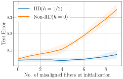
(a)

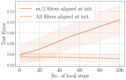
(b)

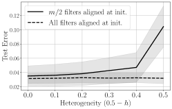
(c)

Figure 2: Empirical results on synthetic dataset to verify the upper bound on test error in Theorem˜2. We fix the training error $\epsilon=0.1$. Figure˜2a: Test error increases as we increase the number of misaligned filters, with much larger rate of increase in the non-IID setting. Figures 2b and 2c: Test error increases with local steps and heterogeneity when $m/2$ filters are misaligned at initialization, remains constant when all the filters are aligned.

3.3 Training Loss Convergence and Test Error Guarantee

Next, we state our main result regarding the convergence of FedAvg with random initialization. We assume the CNN weights are initialized as ${\bf w}_{j,r}^{(0)}\sim\mathcal{N}(\mathbf{0},\sigma_{0}^{2}\mathbf{I}_{d})$ for all filters, where $\mathbf{I}_{d}$ is the $(d\times d)$ identity matrix. We first state the following standard conditions used in our analysis.

Condition 1.

Let $\epsilon$ be a desired training error threshold and $\delta\in(0,1)$ be some failure probability.

1. The allowed number of communication rounds $t$ is bounded by $T^{*}=\frac{1}{\eta}\mathrm{poly}(\epsilon^{-1},m,n,d)$.

2. Dimension $d$ is sufficiently large: $d\gtrsim\max\left\{\tfrac{n\left\|\bm{\mu}\right\|_{2}^{2}}{\sigma_{p}^{2}},n^{2}\right\}$.

3. Training set size $n$ and neural network width $m$ satisfy: $m\gtrsim\log(n/\delta),n\gtrsim\log(m/\delta)$.

4. Standard deviation of Gaussian initialization is sufficiently small: $\sigma_{0}\lesssim\min\left\{\tfrac{\sqrt{n}}{\sigma_{p}d\tau},\tfrac{1}{\left\|\bm{\mu}\right\|_{2}}\right\}$.

5. The norm of the signal satisfies: $\left\|\bm{\mu}\right\|_{2}^{2}\gtrsim\sigma_{p}^{2}$.

6. Learning rate is sufficiently small: $\eta\lesssim\min\left\{\tfrac{nm}{\sigma_{p}^{2}d},\tfrac{1}{\left\|\bm{\mu}\right\|_{2}^{2}},\tfrac{1}{\sigma_{p}^{2}d}\right\}.$

The above conditions are standard and have also been made in (Cao et al., 2022; Kou et al., 2023) for the purpose of theoretical analysis. (C1) is a mild condition needed to ensure that the signal and noise coefficients remain bounded throughout the duration of training. Furthermore, we see in Theorem 1 that we only need $T=\mathcal{O}\left(mn\eta^{-1}\epsilon^{-1}d^{-1}\log(\tau/\epsilon)\right)$ rounds to reach a training error of $\epsilon$, which is well within the admissible number of rounds. (C2) is used to bound the correlation between the noise vectors and also the correlation of the initial filter weights with the signal and noise. (C3) is needed to ensure that a sufficient number of filters have non-zero activations at initialization so that the initial gradient is non-zero. (C4) is needed to ensure that the initial weights of the CNN are not too large and that it has bounded loss for all datapoints. (C5) is needed to ensure that signal learning is not too slow compared to noise memorization. Finally, a small enough learning rate in (C6) ensures that Local GD does not diverge. Additional discussion on these assumptions is provided in Appendix˜C. With this assumption we are now state our main results.

Theorem 1 (Training Loss Convergence).

For any $\epsilon>0$ under ˜1, there exists a $T=\mathcal{O}\left(\frac{mn}{\eta\sigma_{p}^{2}d\tau}\right)+\mathcal{O}\left(\frac{mn\log(\tau/\epsilon)}{\eta\sigma_{p}^{2}d\epsilon}\right)$ such that FedAvg satisfies $L({\bf W}^{(T)})\leq\epsilon$ with probability $\geq 1-\delta$.

Our training error convergence consists of two stages. In the first stage consisting of $T_{1}:=\mathcal{O}\left(\tfrac{mn}{\eta\sigma_{p}^{2}d\tau}\right)$ rounds, we show that the magnitudes of the cross-entropy loss derivatives are lower bounded by a constant, i.e., $|\ell^{\prime}(y_{k,i}f({\bf W}_{k}^{(t,s)},{\bf x}_{k,i}))|=\Omega\left(1\right)$. Using this we can show that the signal and noise coefficients $\{\Gamma_{j,r}^{(t)},\overline{P}_{j,r,k,i}^{(t)}\}$ grow linearly and are $\Theta\left(1\right)$ by the end of this stage. Consequently, by the end of the first stage, the model reaches a neighborhood of a global minimizer where the loss landscape is nearly convex. Then in the second stage, we can establish that the training error consistently decreases to an arbitrary error $\epsilon$ in $\mathcal{O}\left(\tfrac{mn\log(\tau/\epsilon)}{\eta\sigma_{p}^{2}d\epsilon}\right)$ rounds.

Note that our analysis does not require the condition $\eta\propto\nicefrac{{1}}{{\tau}}$ as is common in many works analyzing FedAvg. Therefore, by setting $\tau$ large enough we can make the number of rounds in the first stage as small as $\mathcal{O}\left(1\right)$, thereby reducing the communication cost of FL. However, in the second stage we do not see any continued benefit of local steps; in fact the number of rounds required grows as $\log(\tau)$. This suggests an optimal strategy would be to adapt $\tau$ throughout training: start with large $\tau$ and decrease $\tau$ after some rounds, which has also been found to work well empirically (Wang & Joshi, 2019).

Theorem 2 (Test Error Bound).

Define signal-to-noise ratio $\mathrm{SNR}:=\nicefrac{{\left\|\bm{\mu}\right\|_{2}}}{{\sigma_{p}\sqrt{d}}}$ and $A_{j}:=\{r\in[m]:\langle{\bf w}_{j,r}^{(0)},j\bm{\mu}\rangle\geq 0\}$ to be the set of aligned filters (Definition˜1) corresponding to label $j$. Then under the same conditions as Theorem˜1, our trained CNN achieves

1. When $\mathrm{SNR}^{2}\lesssim\nicefrac{{1}}{{\sqrt{nd}}}$, test error $L_{\mathcal{D}}^{0-1}({\bf W}^{(T)})\geq 0.1$.

2. When $\mathrm{SNR}^{2}\gtrsim\nicefrac{{1}}{{\sqrt{nd}}}$, test error

   $$L_{\mathcal{D}}^{0-1}({\bf W}^{(T)}) \leq\mfrac{1}{2}\textstyle\sum_{j\in\{\pm 1\}}\exp\Big{(}-\mfrac{n}{d}\Big{[}\tfrac{\left|A_{j}\right|}{m}\mathrm{SNR}^{2}$$

   $$+\big{(}1-\tfrac{\left|A_{j}\right|}{m}\big{)}\mathrm{SNR}^{2}\left(h+\tfrac{1}{\tau}(1-h)\right)\Big{]}^{2}\Big{)}.$$

Impact of SNR on harmful/benign overfitting.

Intuitively, if the $\mathrm{SNR}$ is too low ($\mathrm{SNR}^{2}\lesssim\nicefrac{{1}}{{\sqrt{nd}}}$), then there is simply not enough signal strength for the model to learn compared to the noise. Hence, we cannot expect the model to generalize well no matter how we train it. This generalizes the centralized training result in (Kou et al., 2023, Theorem 4.2) (with $p=0$), which corresponds to $\tau=1$ in FedAvg. In this case, the model is in the regime of harmful overfitting. However, if the $\mathrm{SNR}$ is sufficiently large ($\mathrm{SNR}^{2}\gtrsim\nicefrac{{1}}{{\sqrt{nd}}}$), we enter the regime of benign overfitting, where the model can fit the data and generalize well with the test error reducing exponentially with the global dataset size $n$.

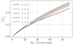
(a) IID Signal Learning

(b) IID Noise Memorization

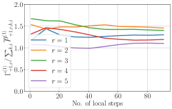
(c) IID Sig. Learning/Noise Mem.

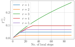
(d) NonIID Signal Learning

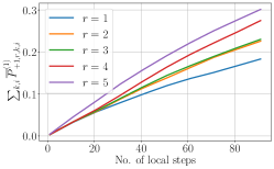
(e) NonIID Noise Memorization

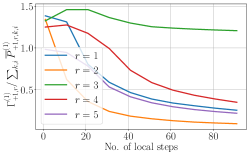
(f) NonIID Sig. Learning/Noise Mem.

Figure 3: Signal learning and noise memorization for our CNN model in the IID $(h=\nicefrac{{1}}{{2}})$ and NonIID $(h=0)$ setting after $1$ round. Figures 3a, 3d: In the IID setting signal learning coefficients are similar for all the filters and increase with the number of local steps $\tau$ but in the NonIID setting they saturate (Lemma˜1) for misaligned filters ($r=1,2,4,5$). Figures 3b, 3e: Noise memorization is similar for all filters in both settings and grows with $\tau$ Lemma˜2. Figures 3c, 3f: in the IID setting, the ratio of signal learning to noise memorization remains independent of $\tau$. But in the NonIID setting, the ratio decreases to zero as $\tau$ increases for misaligned filters ($r=1,2,4,5$).

Empirical Verification.

We now provide empirical verification of the upper bound on the test error in Theorem˜2 in the benign overfitting regime. We simulate a synthetic dataset following our data-generation model in Section˜2, with $n=20$ datapoints, $K=2$ clients and $m=10$ filters. Additional experimental details can be found in Appendix˜F. We fix a training error threshold of $\epsilon=0.1$ and then measure the test error of our CNN under various settings in Figure˜2. Figure˜2a shows the test error as a function of the number of misaligned filters ($m-|A_{j}|$ in Theorem˜2) under different data partitionings with the number of local steps fixed at $\tau=100$. While the test error grows with the number of misaligned filters in both data settings, the rate of growth is much larger in the non-IID setting. Figure˜2b shows the test error as a function of local steps $\tau$ under different initializations for fixed $h=0$ while Figure˜2c shows the test error as a function of heterogeneity under different initializations for fixed $\tau=100$. As predicted by our theory, heterogeneity and the number of local steps do not affect test error when all the filters are aligned at initialization. On the other hand, the test error grows with $\tau$ and heterogeneity when the number of misaligned filters is non-zero ($m/2=5$) for each $j\in\{\pm 1\}$. Therefore, our empirical results strongly validate our theoretical results showing the effect of heterogeneity, number of local steps and number of misaligned filters on the test error.

3.4 Impact of Filter Alignment and Data Heterogeneity on Signal Learning and Noise Memorization.

The key results in our analysis are the following lemmas which bound the growth of the signal learning and noise coefficient during the first stage of training, that is $0\leq t\leq T_{1}$ (see discussion under Theorem˜1). Using our definition of $A_{j}:=\{r\in[m]:\langle{\bf w}_{j,r}^{(0)},j\bm{\mu}\rangle\geq 0\}$ as the set of aligned filters, we have the following lemma for growth of the signal learning coefficient in the first stage.

Lemma 1.

Under ˜1, for all $0\leq t\leq T_{1}$, we have $\Gamma_{j,r}^{(t)}=\Omega\left(\frac{t\eta\left\|\bm{\mu}\right\|_{2}^{2}\tau}{m}\right)$ if $r\in A_{j}$ and $\Gamma_{j,r}^{(t)}=\Omega\left(\frac{t\eta\left\|\bm{\mu}\right\|_{2}^{2}(1+h(\tau-1))}{m}\right)$ if $r\notin A_{j}$.

This lemma shows that for aligned filters ($r\in A_{j}$), $\Gamma_{j,r}^{(t)}$ does not depend on heterogeneity and grows linearly with the number of local steps $\tau$. On the other hand, for misaligned filters $(r\notin A_{j})$, the growth depends on the heterogeneity parameter $h$. Furthermore, under extreme data heterogeneity ($h=0$), for misaligned filters $\Gamma_{j,r}^{(t)}$ does not scale with the number of local steps $\tau$. For the growth of noise coefficients we have the following corresponding lemma,

Lemma 2.

Under ˜1, for all $0\leq t\leq T_{1}$ we have $\sum_{k,i}\overline{P}_{j,r,k,i}^{(t)}=\Theta\left({\mfrac{t\eta\tau\sigma_{p}^{2}d}{m}}\right).$

This lemma shows that noise memorization does not depend on data-heterogeneity or filter alignment and always scales linearly with the number of local steps $\tau$. Intuitively, this can be expected because the noise vectors are independent of the label information $y$ in a datapoint following our data generation model in Section˜2 and for any given filter we can show there are $\Omega\left(N\right)$ noise vectors that are aligned with the filter at initialization for every client with high probability (see Lemma˜7).

Using the above two lemmas, we have the following bound on the ratio of signal learning to noise memorization for filter $(j,r)$ at the end of the first stage of training

$$\mfrac{\Gamma_{j,r}^{(T_{1})}}{\sum_{k,i}\overline{P}_{j,r,k,i}^{(T_{1})}}\geq\begin{cases}\mathrm{SNR}^{2},\text{ if }r\in A_{j},\\ \mathrm{SNR}^{2}(h+\frac{1}{\tau}(1-h)),\text{ if }r\in[m]\setminus A_{j}.\end{cases}$$ (6)

This ratio is key to bounding the generalization performance of the CNN model as we show later in the proof of Theorem˜2 in Section˜D.1. For aligned filters ($r\in A_{j}$), the ratio is unaffected by data heterogeneity $h$ and the number of local steps $\tau$. However, for misaligned filters ($r\in[m]\setminus A_{j}$), the ratio becomes smaller as heterogeneity increases ($h$ becomes smaller) or $\tau$ increases. Thus, for misaligned filters we see a corresponding dependence on heterogeneity and local steps in our upper bound on test error in Theorem˜2. Note that in centralized training with $\tau=1$, we have $(h+\frac{1}{\tau}(1-h))=1$ and thus we do not see any impact of heterogeneity at misaligned filters. Therefore, we recover the bound $L_{\mathcal{D}}^{0-1}({\bf W}^{(T)})\leq\exp(-n\mathrm{SNR}^{2}/d)$ in (Kou et al., 2023, Theorem 4.2). It is only in FL training with $\tau>1$ local steps that we encounter the adverse effect of data heterogeneity at the misaligned filters.

Empirical Verification.

We empirically verify the results above in the IID $(h=1/2)$ and Non-IID $(h=0)$ setting following the same simulation setup as done in Figure˜2. Figure Figure˜3a shows that in the IID setting signal learning coefficients are similar for all the filters and increases with the number of local step. However, as shown by Figure˜3d, in the NonIID setting signal learning saturates for misaligned filters. Figures 3b and 3e show that the growth of noise coefficients for all the filters is similar in the IID and non-IID case.

Figure 4: Initial alignment of the filters in Section˜3.3.

In Figure˜3c we see that ratio of signal learning to noise memorization is lower bounded by a constant for all filters in the IID setting whereas in the Non-IID setting it decays as $\tau$ increases for misaligned filters (Figure˜3f), thus verifying our theoretical analysis.

3.5 Impact of Pre-Training on Federated Learning

Given the result in Theorem˜2, we return to our question in Section˜1, about the effect of pre-trained initialization on improving generalization performance in FL. We focus on centralized pre-training but our discussion here can be extended to federated pre-training as well (see Lemma˜31 which states a federated counterpart of the lemma below).

Suppose we pre-train a CNN model in a centralized manner on a dataset with signal $\bm{\mu}^{(\text{pre})}$ generated according to the data model described in Section˜2. Now if we train for sufficient number of iterations, then we can show that all filters will be correctly aligned with the pre-training signal.

Lemma 3 (All Filters Aligned After Sufficient Training).

There exists $T_{1}=\mathcal{O}\left(\frac{mn}{\eta\sigma_{p}^{2}d}\right)$ such that for all $t\geq T_{1},j\in\{\pm 1\},r\in[m]$ we have $\langle{\bf w}^{(\text{pre},t)}_{j,r},j\bm{\mu}^{(\text{pre})}\rangle\geq 0$.

Now suppose we pre-train for $t\geq T_{1}$ iterations to get a model ${\bf W}^{(\text{pre},*)}$ and use this model to initialize for downstream federated training (i.e., ${\bf W}^{(0)}={\bf W}^{(\text{pre, *})}$) with signal vector $\bm{\mu}$. Then for all $j,r$ filters, we have $\langle{\bf w}_{j,r}^{(0)},j\bm{\mu}\rangle=\langle{\bf w}^{(\text{pre,*})}_{j,r},j\bm{\mu}^{(\text{pre})}\rangle+\langle{\bf w}^{(\text{pre,*})}_{j,r},j(\bm{\mu}-\bm{\mu}^{(\text{pre})})\rangle$. We also know that $\langle{\bf w}^{(\text{pre,*})}_{j,r},j\bm{\mu}^{(\text{pre})}\rangle\geq 0$ using Lemma˜3. Therefore, if $\|\bm{\mu}-\bm{\mu}^{(\text{pre})}\|_{2}$ is small, all the filters $\{{\bf w}_{j,r}^{(0)}\}$ are correctly aligned with the signal $j\bm{\mu}$. As a result, in Theorem˜2 $A_{j}=[m]$ for $j\in\{\pm 1\}$ and in the benign overfitting regime ($\mathrm{SNR}^{2}\gtrsim\nicefrac{{1}}{{\sqrt{nd}}}$), we recover the centralized result $L_{\mathcal{D}}^{0-1}({\bf W}^{(T)})\leq\exp(-n\mathrm{SNR}^{2}/d)$ (Kou et al., 2023, Theorem 4.2). Hence, the adverse effects of cross-client heterogeneity are mitigated with pre-trained initialization.

4 Experiments

In this section we provide empirical results showing how our insights from Section˜3 extend to practical FL training on real world datasets with deep CNN models. Unless specified otherwise, we use the ResNet18 model (He et al., 2016) in all our experiments and split the data across $20$ clients using the Dirichlet sampling scheme (Hsu et al., 2019) with non-iid parameter $\alpha=0.3$. For pre-training, we use a ResNet18 pre-trained on ImageNet (Russakovsky et al., 2015), available in PyTorch (Paszke et al., 2019). Additional experimental details can be found in Appendix˜F.

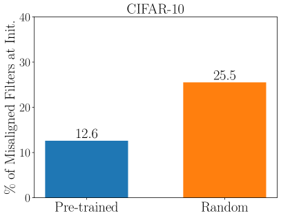
(a)

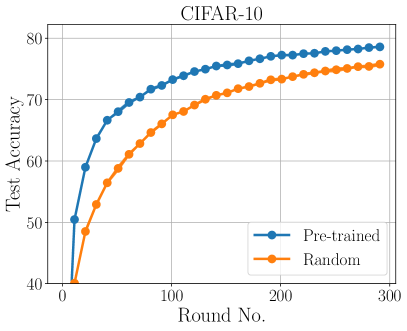
(b)

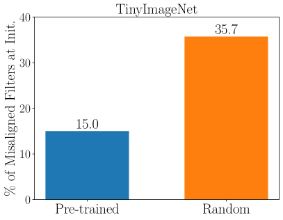
(c)

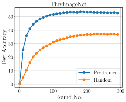
(d)

Figure 5: The percentage of misaligned filters (see Equation˜7 and test accuracy for different initializations on CIFAR-10 (Figure˜5a and Figure˜5b) and TinyImageNet (Figure˜5c and Figure˜5d). As the complexity of the signal information in the data grows from CIFAR-10 to TinyImageNet, we see a sharp increase in the ratio of misaligned filters for random initialization, explaining why pre-trained initialization offers larger improvements for TinyImageNet.

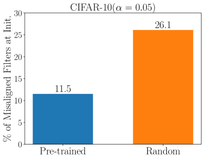
(a)

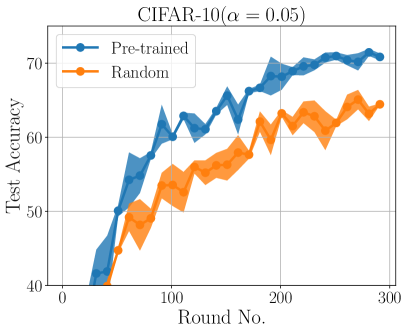
(b)

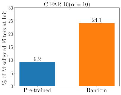
(c)

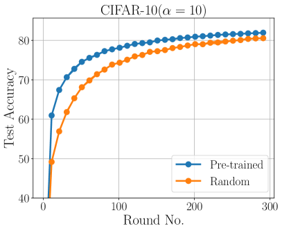
(d)

Figure 6: The percentage of misaligned filters (see Equation˜7) and test accuracy for different initializations on CIFAR-10 with $\alpha=0.05$ heterogeneity (Figure˜6a and Figure˜6b) and $\alpha=10$ heterogeneity (Figure˜6c and Figure˜6d). Although the percentage of misaligned filters does not vary significantly across the two settings for both initializations (signal information is the same in both settings), pre-training offers more improvement in the higher heterogeneity setting ($\alpha=0.05)$, as suggested by our theoretical analysis.

Empirical Measure of Misalignment.

Measuring filter alignment for deep CNNs is challenging since we cannot explicitly characterize the signal information present in real world datasets and furthermore different layers will learn the signal at different levels of granularity. Nonetheless, our theoretical findings suggest that given sufficient number of training rounds, filters will be aligned with the signal (see Section˜3) and once a filter is aligned, the sign of the output produced by the filter with respect to the signal does not change, i.e, if $\langle{\bf w}_{j,r}^{(t)},j\bm{\mu}\rangle>0$ then $\mathrm{sign}(\langle{\bf w}_{j,r}^{(t^{\prime})},\bm{\mu}\rangle)=\mathrm{sign}(\langle{\bf w}_{j,r}^{(t)},\bm{\mu}\rangle)$, for all $t^{\prime}\geq t$. Therefore, we propose to use the sign of the output produced by a filter at the end of training as a reference for alignment at any given round. Formally, let ${\bf W}^{(0)},{\bf W}^{(1)}\cdots{\bf W}^{(T)}$ be the sequence of iterates produced by federated training and let $\mathcal{F}({\bf w},{\bf x})=[\langle{\bf w},{\bf x}(1)\rangle,\langle{\bf w},{\bf x}(2)\rangle,\dots\langle{\bf w},{\bf x}(p)\rangle]\in\mathbb{R}^{p}$ be the feature map vector generated by filter ${\bf w}$ for input ${\bf x}$. For a given batch of data $\mathcal{B}$, we define the empirical measure of alignment of filter ${\bf w}^{(t)}$ relative to ${\bf w}^{(T)}$ as follows:

$$\mathcal{A}({\bf w}^{(t)}):=\sum_{x\in\mathcal{B},l\in[p]}\mathrm{sign}(\mathcal{F}_{l}({\bf w}^{(t)},{\bf x}))\mathrm{sign}(\mathcal{F}_{l}({\bf w}^{(T)},{\bf x})).$$ (7)

We say that the weight ${\bf w}^{(t)}$ at round $t$ is misaligned if $\mathcal{A}({\bf w}^{(t)})<0$, because this implies that the sign of the output produced by the filter ${\bf w}$ at round $t$ eventually changed for a majority of the inputs, hence indicating that the filter was misaligned at round $t$. We compute this measure over a batch of data to account for signal information coming from different classes of data as well as reduce the impact of noise in the data.

Measuring Misalignment on Real World Datasets with Varying Signal Information.

In this experiment our goal is to empirically demonstrate that (a) pre-trained initialization leads to much fewer number of misaligned filters than random initialization and (b) the number of misaligned filters for random initialization increases as we increase the complexity of the signal. To demonstrate this, we consider federated training on the 1. CIFAR-10 (Krizhevsky, 2009) and 2. TinyImageNet (Le & Yang, 2015) datasets. Section˜4 shows the test accuracy and percentage of misaligned filter across training rounds for both datasets with pre-trained and random initialization. Firstly, we see that the percentage of misaligned filters is $2-3\times$ smaller when starting from a pre-trained initialization compared to a random initialization. Furthermore, as the complexity of the signal information in the dataset increases (CIFAR-10 < TinyImageNet), we see a sharp increase in the percentage of misaligned filters ($25\%$ to $40\%$) for random initialization. In contrast, with pre-trained initialization, the percentage of misaligned filters remains less than $15\%$ across datasets leading to a larger improvement in test accuracy for TinyImageNet. These results align with our theoretical findings: as the ratio of misaligned filters increases, the benefits of pre-training become more pronounced.

Measuring Misalignment with Varying Heterogeneity Levels.

We extend the experiment in Section˜4 conducted on CIFAR-10 with $\alpha=0.3$ Dirichlet heterogeneity to other levels of heterogeneity 1. $\alpha=0.05$ which is an extreme non-IID split and 2. $\alpha=10$ which can be thought of as close to IID split. Section˜4 shows the test accuracy and percentage of misaligned filters plots for these two heterogeneity levels with pre-trained and random initialization. We observe that in both cases the percentage of misaligned filters remains approximately $25\%$ with random initialization and $10\%$ with pre-trained initialization, regardless of the level of heterogeneity. However, as heterogeneity increases, the improvement in test accuracy provided by pre-trained initialization becomes more pronounced. This trend is consistent with our theoretical analysis in Theorem 2, which suggests that the percentage of misaligned filters will have a greater impact on test performance as data heterogeneity increases.

5 Conclusion and Future Work

In this work we provide a deeper theoretical explanation for why pre-training can drastically reduce the adverse effects of non-IID data in FL by studying the class of two layer CNN models under a signal-noise data model. Our analysis shows that the reduction in test accuracy seen in non-IID FL compared to IID FL is only caused by filters that are misaligned at initialization. When starting from a pre-trained model we expect most of the filters to be already aligned with the signal thereby reducing the effect of heterogeneity and leading to a higher ratio of signal learning to noise memorization. This is corroborated by experiments on synthetic setup as well as more practical FL training tasks. Our work also opens up several avenues for future work. These including extending the analysis to deeper and more practical neural networks and also incorporating multi-class classification with more than two labels. Another interesting direction is to see how pre-training affects other federated algorithms such as those that explicitly incorporate heterogeneity reducing mechanisms.

[sections] [sections]l1

Appendix A Additional Related Work

Use of Pre-Trained Models in Federated Learning.

(Tan et al., 2022) explore the benefit of using pre-trained models in FL by proposing to use multiple fixed pre-trained backbones as the encoder model at each client and using contrastive learning to extract useful shared representations. (Zhuang et al., 2023) discuss the opportunities and challenges of using large foundation models for FL including the high communication and computation cost. One solution to this as proposed by (Legate et al., 2024) is that instead of full fine-tuning as done in (Chen et al., 2022; Nguyen et al., 2022), we can just fine-tune the last layer. Specifically (Legate et al., 2024) proposes a two-stage approach to federated fine-tuning by first fine-tuning the head and then doing a full-finetuning. This approach is inspired by results in the centralized setting (Kumar et al., 2022) which show that in some case fine-tuning can distort the pre-trained features. (Fanì et al., 2023) also study the problem of fine-tuning just the last layer in a federated setting by replacing the softmax classifier with a ridge-regression classifier which enables them to compute a closed form expression for the last layer weights.

There has also been some recent work on exploring the benefit of pre-training for federated natural language processing tasks including the use of Large Language Models (LLMs). (Wang et al., 2023) discuss how to leverage the power of pre-trained LLMs for private on-device fine-tuning of language models. Specifically, (Wang et al., 2023) proposes a distribution matching approach to select public data that is closest to private data and then use this selected public data to train the on-device language model. (Zhang et al., 2023) propose to first pre-train on synthetic data to construct the initialization point followed by federated fine-tuning. (Hou et al., 2024) propose that clients send DP information to the server which then uses this information to generate synthetic data and fine-tune centrally on this synthetic data. (Liu & Miller, 2020) discuss the challenges of pre-training and fine-tuning BERT in federated manner using clinical notes from multiple silos without data transfer. (Tian et al., 2022) propose to pre-train a BERT model in a federated manner in a more general setting and show that their pre-trained model can retain accuracy on the GLUE (Wang et al., 2018) dataset without sacrificing client privacy. Xu et al. (2023b) pretrain production on-device language models on public web data before fine-tuning in federated learning with differential privacy, and Wu et al. (2024) later replace the pretraining data with data synthesized by LLMs. (Gupta et al., 2022) propose a defense using pre-trained models to prevent an attacker from recovering multiple sentences from gradients in the federated training of the language modeling task.

Importance of Initialization for Private Optimization.

We note that an orthogonal line of work has explored the benefits of starting from a pre-trained model when doing differentially private optimization (Dwork et al., 2006) and seen similar striking improvement in accuracy (De et al., 2022; Li et al., 2022b; Yu et al., 2022; Xu et al., 2023a), as we see in the heterogeneous FL setting. (Ganesh et al., 2023) study this phenomenon for a stylized mean estimation problem and show that public pre-training can help the model start from a good loss basin which is otherwise hard to achieve with private noisy optimization. (Li et al., 2022a) study differentially private convex optimization and show that starting from a pre-trained model can leads to dimension independent convergence guarantees. Specifically (Li et al., 2022a) define the notion of restricted Lipschitz continuity and show that when gradients are low rank most of the restricted Lispchitz coefficients will be zero. (Ye et al., 2023) studies the impact of different random initializations on the privacy bound when training overparameterized neural networks and shows that for some initializations (LeCun (LeCun et al., 2012), Xavier (Glorot & Bengio, 2010)) the privacy bound improves with increasing depth while for other initializations (He (He et al., 2015), NTK (Allen-Zhu & Li, 2023)) it degrades with increasing depth.

Generalization performance in Federated Learning.

Several existing works have studied the generalization performance of FL in different settings (Cheng et al., 2021; Gholami & Seferoglu, 2024; Huang et al., 2023; Yuan et al., 2021). Some of the initial works either provide results independent of the algorithm being used (Mohri et al., 2019; Hu et al., 2022; Sun & Wei, 2022), or only study convex losses (Chen et al., 2021; Fallah et al., 2021). (Barnes et al., 2022; Sefidgaran et al., 2022) derive information-theoretic bounds, but these bounds require specific forms of loss functions and cannot capture effects of heterogeneity. (Huang et al., 2021) study the generalization of FedAvg on wide two-layer ReLU networks with homogeneous data. (Collins et al., 2022) studies FedAvg under multi-task linear representation learning setting. In (Sun et al., 2024), the authors have demonstrated the impact of data heterogeneity on the generalization performance of some popular FL algorithms.

Appendix B Theory Notation and Preliminaries

We follow a similar notation as (Kou et al., 2023) in most of the analysis.

Table 1: Summary of notation

Symbol	Description
$j\in\{-1,1\}$	Layer index
$m$	Number of filters
$d$	Dimension of filter
$r\in[m]$	Filter Index
$K$	Number of clients
$k\in[K]$	Client index
$N$	Number of datapoints at each client
$i\in[N]$	Datapoint index
$n=KN$	Global dataset size
$y_{k,i}\in\{1,-1\}$	Label of $i$-th datapoint at $k$-th client
$\bm{\mu}$	Signal vector
$\sigma_{p}^{2}$	Variance of Gaussian noise
$\bm{\xi}_{k,i}$	Noise vector for $k$-th client and $i$-th datapoint
$\eta$	Local learning rate
$\tau$	Number of local steps
$\ell(z)=\log(1+\exp(-z))$	Cross-entropy loss function
$\sigma(z)=\max(0,z)$	ReLU function
$\sigma^{\prime}(z)=\mathds{1}\big{(}z\geq 0\big{)}$	Derivative of ReLU function
$t$	Round index
$s$	Iteration index
$h$	Heterogeneity parameter
$\mathrm{SNR}:=\nicefrac{{\left\|\bm{\mu}\right\|_{2}}}{{\sigma_{p}\sqrt{d}}}$	Signal to Noise Ratio
${\bf W}_{k}^{(\cdot,\cdot)}$	Parameterized weights of the $k$-th client
${\bf w}_{j,r,k}^{(\cdot,\cdot)}$	$(j,r)$-th filter weight of the $k$-th client
$\gamma_{j,r,k}^{(\cdot,\cdot)}$	Local signal co-efficient for $k$-th client
$\rho_{j,r,k,i}^{(\cdot,\cdot)}$	Local noise coefficient for $k$-th client and $i$-th datapoint
$\overline{\rho}_{j,r,k,i}^{(\cdot,\cdot)}$	Positive local noise coefficient for $k$-th client and $i$-th datapoint
$\underline{\rho}_{j,r,k,i}^{(t,s)}$	Negative local noise coefficient for $k$-th client and $i$-th datapoint
${\ell^{\prime}}_{k,i}^{(\cdot,\cdot)}$	Shorthand for $-1/\left(1+\exp(y_{k,i}f({\bf W}_{k}^{(\cdot,\cdot)},{\bf x}_{k,i})\right)$ which is the
	derivative of cross-entropy loss for $i$-th datapoint at $k$-th client
${\bf W}^{(\cdot)}$	Parameterized weight vector of the global model
${\bf w}_{j,r}^{(\cdot)}$	$j,r$-th filter weight of the global model
$\Gamma_{j,r}^{(\cdot)}$	Global signal co-efficient
$P_{j,r,k,i}^{(\cdot)}$	Global noise coefficient for $(k,i)$-th datapoint
$\overline{P}_{j,r,k,i}^{(\cdot)}$	Positive global noise coefficient for $(k,i)$-th datapoint
$\underline{P}_{j,r,k,i}^{(\cdot)}$	Negative global noise coefficient for $(k,i)$-th client datapoint

B.1 Local Model Update

Using local GD updates in equation 4 to minimize the local loss function in equation 2, the local model update for the $(j,r)$ filter at client $k$ in round $t$ can be written as,

$${\bf w}_{j,r,k}^{(t,\tau)} ={\bf w}_{j,r}^{(t)}-\frac{\eta}{Nm}\sum_{s=0}^{\tau-1}\sum_{i\in[N]}{\ell^{\prime}}_{k,i}^{(t,s)}\cdot\sigma^{{}^{\prime}}\big{(}\langle{\bf w}_{j,r,k}^{(t,s)},\bm{\xi}_{k,i}\rangle\big{)}\cdot jy_{k,i}\bm{\xi}_{k,i}$$

$$\hskip 10.0pt-\frac{\eta}{Nm}\sum_{s=0}^{\tau-1}\sum_{i\in[N]}{\ell^{\prime}}_{k,i}^{(t,s)}\cdot\sigma^{{}^{\prime}}\big{(}\langle{\bf w}_{j,r,k}^{(t,s)},y_{k,i}\bm{\mu}\rangle\big{)}\cdot j\bm{\mu}$$

$$={\bf w}_{j,r}^{(t)}+j\gamma_{j,r,k}^{(t,\tau)}\cdot\left\|\bm{\mu}\right\|_{2}^{-2}\cdot\bm{\mu}+\sum_{i\in[N]}\rho_{j,r,k,i}^{(t,\tau)}\cdot\left\|\bm{\xi}_{k,i}\right\|_{2}^{-2}\cdot\bm{\xi}_{k,i}$$ (47)

where, we use ${\bf w}_{j,r,k}^{(t,0)}\triangleq{\bf w}_{j,r}^{(t)}$. Further, we define

$$\gamma_{j,r,k}^{(t,\tau)} \triangleq-\frac{\eta}{Nm}\sum_{s=0}^{\tau-1}\sum_{i\in[N]}{\ell^{\prime}}_{k,i}^{(t,s)}\cdot\sigma^{{}^{\prime}}\big{(}\langle{\bf w}_{j,r,k}^{(t,s)},y_{k,i}\bm{\mu}\rangle\big{)}\cdot\left\|\bm{\mu}\right\|_{2}^{2},$$ (48)

$$\rho_{j,r,k,i}^{(t,\tau)} \triangleq-\frac{\eta}{Nm}\sum_{s=0}^{\tau-1}{\ell^{\prime}}_{k,i}^{(t,s)}\cdot\sigma^{{}^{\prime}}\big{(}\langle{\bf w}_{j,r,k}^{(t,s)},\bm{\xi}_{k,i}\rangle\big{)}\cdot\left\|\bm{\xi}_{k,i}\right\|_{2}^{2}\cdot jy_{k,i}.$$ (49)

which respectively, denote the local signal $(\gamma_{j,r,k}^{(t,\tau)})$ and local noise $(\{\rho_{j,r,k,i}^{(t,\tau)}\}_{i})$ components of ${\bf w}_{j,r,k}^{(t,\tau)}$. We also define $\overline{\rho}_{j,r,k,i}^{(t,\tau)}=\rho_{j,r,k,i}^{(t,\tau)}\mathds{1}\big{(}\rho_{j,r,k,i}^{(t,\tau)}\geq 0\big{)}$ and $\underline{\rho}_{j,r,k,i}^{(t,\tau)}=\rho_{j,r,k,i}^{(t,\tau)}\mathds{1}\big{(}\rho_{j,r,k,i}^{(t,\tau)}<0\big{)}$, where $\mathds{1}\big{(}\cdot\big{)}$ denotes the indicator function, and which can alternatively be written as

$$\overline{\rho}_{j,r,k,i}^{(t,\tau)}=-\frac{\eta}{Nm}\sum_{s=0}^{\tau-1}{\ell^{\prime}}_{k,i}^{(t,s)}\cdot\sigma^{{}^{\prime}}\big{(}\langle{\bf w}_{j,r,k}^{(t,s)},\bm{\xi}_{k,i}\rangle\big{)}\cdot\left\|\bm{\xi}_{k,i}\right\|_{2}^{2}\cdot\mathds{1}\big{(}y_{k,i}=j\big{)},$$ (50)

$$\underline{\rho}_{j,r,k,i}^{(t,\tau)}=\frac{\eta}{Nm}\sum_{s=0}^{\tau-1}{\ell^{\prime}}_{k,i}^{(t,s)}\cdot\sigma^{{}^{\prime}}\big{(}\langle{\bf w}_{j,r,k}^{(t,s)},\bm{\xi}_{k,i}\rangle\big{)}\cdot\left\|\bm{\xi}_{k,i}\right\|_{2}^{2}\cdot\mathds{1}\big{(}y_{k,i}=-j\big{)}.$$ (51)

B.2 Proof of Proposition˜1

The global model update at round $t+1$ can be written as

$${\bf w}_{j,r}^{(t+1)} =\sum_{k=1}^{K}\frac{1}{K}{\bf w}_{j,r,k}^{(t,\tau)}$$

$$={\bf w}_{j,r}^{(t)}+\frac{j}{K}\sum_{k=1}^{K}\gamma_{j,r,k}^{(t,\tau)}\cdot\left\|\bm{\mu}\right\|_{2}^{-2}\cdot\bm{\mu}+\sum_{k=1}^{K}\sum_{i\in[N]}\frac{1}{K}\rho_{j,r,k,i}^{(t,\tau)}\cdot\left\|\bm{\xi}_{k,i}\right\|_{2}^{-2}\cdot\bm{\xi}_{k,i}.$$ (52)

Mimicking the signal-noise decomposition in equation 47, we can define a similar decomposition for the global model as follows.

$${\bf w}_{j,r}^{(t)}={\bf w}_{j,r}^{(0)}+j\Gamma_{j,r}^{(t)}\cdot\left\|\bm{\mu}\right\|_{2}^{-2}\cdot\bm{\mu}+\sum_{k=1}^{K}\sum_{i\in[N]}P_{j,r,k,i}^{(t)}\cdot\left\|\bm{\xi}_{k,i}\right\|_{2}^{-2}\cdot\bm{\xi}_{k,i}.$$ (53)

B.3 Co-efficient Update Equations

Comparing with equation 52, we have the following recursive update for the global signal and noise coefficients using $n=KN$.

$$\Gamma_{j,r}^{(t+1)} =\Gamma_{j,r}^{(t)}+\sum_{k=1}^{K}\frac{1}{K}\gamma_{j,r,k}^{(t,\tau)}$$

$$=\Gamma_{j,r}^{(t)}-\frac{\eta}{nm}\sum_{k=1}^{K}\sum_{i\in[N]}\sum_{s=0}^{\tau-1}{\ell^{\prime}}_{k,i}^{(t,s)}\cdot\sigma^{{}^{\prime}}\big{(}\langle{\bf w}_{j,r,k}^{(t,s)},y_{k,i}\bm{\mu}\rangle\big{)}\cdot\left\|\bm{\mu}\right\|_{2}^{2}$$ (54)

$$P_{j,r,k,i}^{(t+1)} =P_{j,r,k,i}^{(t)}+\frac{1}{K}\rho_{j,r,k,i}^{(t,\tau)}$$

$$=P_{j,r,k,i}^{(t)}-\frac{\eta}{nm}\sum_{s=0}^{\tau-1}{\ell^{\prime}}_{k,i}^{(t,s)}\cdot\sigma^{{}^{\prime}}\big{(}\langle{\bf w}_{j,r,k}^{(t,s)},\bm{\xi}_{k,i}\rangle\big{)}\cdot\left\|\bm{\xi}_{k,i}\right\|_{2}^{2}\cdot jy_{k,i}.$$ (55)

Analogously, we can also define the positive and negative global noise coefficients,

$$\overline{P}_{j,r,k,i}^{(t+1)}=\overline{P}_{j,r,k,i}^{(t)}-\frac{\eta}{nm}\sum_{s=0}^{\tau-1}{\ell^{\prime}}_{k,i}^{(t,s)}\cdot\sigma^{{}^{\prime}}\big{(}\langle{\bf w}_{j,r,k}^{(t,s)},\bm{\xi}_{k,i}\rangle\big{)}\cdot\left\|\bm{\xi}_{k,i}\right\|_{2}^{2}\mathds{1}\big{(}y_{k,i}=j\big{)}$$ (56)

and,

$$\underline{P}_{j,r,k,i}^{(t+1)}=\underline{P}_{j,r,k,i}^{(t)}+\frac{\eta}{nm}\sum_{s=0}^{\tau-1}{\ell^{\prime}}_{k,i}^{(t,s)}\cdot\sigma^{{}^{\prime}}\big{(}\langle{\bf w}_{j,r,k}^{(t,s)},\bm{\xi}_{k,i}\rangle\big{)}\cdot\left\|\bm{\xi}_{k,i}\right\|_{2}^{2}\mathds{1}\big{(}y_{k,i}=-j\big{)}.$$ (57)

Lemma 4.

(Measuring local and global signal coefficient)

From equation 47, it follows that

$$\langle{\bf w}_{j,r,k}^{(t,s)}-{\bf w}_{j,r}^{(t)},y_{k,i}\bm{\mu}\rangle=jy_{k,i}\gamma_{j,r,k}^{(t,s)}.$$ (58)

and from equation 53, it follows that

$$\langle{\bf w}_{j,r}^{(t)}-{\bf w}_{j,r}^{(0)},\bm{\mu}\rangle=j\Gamma_{j,r}^{(t)}.$$ (59)

Since $\{\Gamma_{j,r}^{(t)}\}_{t}$ are non-negative and non-decreasing in $t$, the global weights $\{{\bf w}_{j,r}^{(t)}\}_{r}$ become increasing aligned with the actual signal $y_{k,i}\bm{\mu}$ corresponding to the filters $j=y_{k,i}$. Similarly, as $\{\gamma_{j,r,k}^{(t,s)}\}_{t}$ are non-negative and non-decreasing in $s$ for fixed $t$, the local weights $\{{\bf w}_{y_{k,i},r,k}^{(t,s)}\}_{r}$ become increasing aligned with the signal $y_{k,i}\bm{\mu}$ corresponding to the filters $j=y_{k,i}$.

Appendix C Training Error Convergence of FedAvg with Random Initialization

For the sake of completeness, we state the conditions used in our analysis (˜1) in full detail.

Assumptions.

Let $\epsilon$ be a desired training error threshold and $\delta\in(0,1)$ be some failure probability. Let $T^{*}=\frac{1}{\eta}\mathrm{poly}(\epsilon^{-1},m,n,d)$ be the maximum admissible rounds.

Suppose there exists a sufficiently large constant $C$, such that the following hold.

Assumption 1.

Dimension $d$ is sufficiently large, i.e.,

$$d\geq C\max\left\{\mfrac{n\left\|\bm{\mu}\right\|_{2}^{2}\log(T^{*}\tau)}{\sigma_{p}^{2}},n^{2}\log(nm/\delta)(\log(T^{*}\tau))^{2}\right\}.$$

Assumption 2.

Training sample size $n$ and neural network width $m$ satisfy

$$m\geq C\log(n/\delta),n\geq C\log(m/\delta).$$

Assumption 3.

The norm of the signal satisfies,

$$\left\|\bm{\mu}\right\|_{2}^{2}\geq C\sigma_{p}^{2}\log(n/\delta).$$

Assumption 4.

Standard deviation of Gaussian initialization is sufficiently small, i.e.,

$$\sigma_{0}\leq\mfrac{1}{C}\min\left\{\mfrac{\sqrt{n}}{\sigma_{p}d\tau},\mfrac{1}{\sqrt{\log(m/\delta)}\left\|\bm{\mu}\right\|_{2}}\right\}.$$

Assumption 5.

Learning rate is sufficiently small, i.e.,

$$\eta\leq\mfrac{1}{C}\min\left\{\mfrac{nm\sqrt{\log(m/\delta)}}{\sigma_{p}^{2}d},\mfrac{1}{\left\|\bm{\mu}\right\|_{2}^{2}},\mfrac{1}{\sigma_{p}^{2}d}\right\}.$$

The assumptions are primarily used to ensure that the model is sufficiently overparameterized, i.e., training loss can be made arbitrarily small, and that we do not begin optimization from a point where the gradient is already zero or unbounded. We provide a more intuitive reasoning behind each of the assumptions below:

• Bounded number of communication rounds: This is needed to ensure that the magnitude of filter weights remains bounded throughout training since they grow logarithmically with the number of updates (see Theorem 3). We note that this is quite a mild condition since the max rounds can have polynomial dependence on $1/\epsilon$ where $\epsilon$ is our desired training error.

• Dimension $d$ is sufficiently large: This is needed to ensure that the model is sufficiently overparameterized and the training loss can be made arbitrarily small. Recall that our input $\mathbf{x}$ consists of a signal component $\bm{\mu}\in\mathbb{R}^{d}$ that is common across all datapoints and noise component $\bm{\xi}\in\mathbb{R}^{d}$ that is independently drawn from $\mathcal{N}(0,\sigma_{p}^{2}\cdot\bm{I})$. Having a sufficiently large $d$ ensures that the correlation between any two noise vectors, i.e. $\langle\bm{\xi},\bm{\xi}^{\prime}\rangle/\|\bm{\xi}\|^{2}$ is not too large. Otherwise if the correlation between two noise vectors is large and negative, then minimizing the loss on one data point could end up increasing the loss on another training point which complicates convergence and prevents loss from becoming arbitrarily small.

• Training set size and network width is sufficiently large: The condition ensures that a sufficient number of filters get activated at initialization with high probability (see Lemma 6 and Lemma 7) and prevents cases where the initial gradient is zero. The condition on training set size also ensures that there are a sufficient number of datapoints with negative and positive labels (see Lemma 8).

• Standard deviation of Gaussian random initialization is sufficiently small: This condition is needed to ensure that the magnitude of the initial correlation between the filter weights and the signal and noise components, i.e $|\langle\mathbf{w}_{j,r}^{(0)},\bm{\mu}\rangle|$, $|\langle\mathbf{w}_{j,r}^{(0)},\bm{\xi}\rangle|$ is not too large. This simplifies the analysis and prevents cases where none of the filters get activated at initialization (see Lemma 21). It also ensures that after some number of rounds all filters get aligned with the signal (see Lemma 30).

• Norm of signal is larger than noise variance: This condition is needed to ensure that all misaligned filters at initialization eventually become aligned with the signal after some rounds (see Lemma 30). This allows us to derive a meaningful bound on test performance that is not dominated by noise memorization.

• Learning rate is sufficiently small: This is a standard condition to ensure that gradient descent does not diverge. The conditions are derived from ensuring that the signal and noise coefficient remain bounded in the first stage of training and that the loss decreases monotonically in every round in the second stage of training.

For ease of reference, we restate Theorem˜1 below.

Theorem (Training Loss Convergence).

Let $T_{1}=\mathcal{O}\left(\frac{mn}{\eta\sigma_{p}^{2}d\tau}\right)$. With probability $1-\delta$ over the random initialization, for all $T_{1}\leq T\leq T^{*}$ we have,

$$\frac{1}{T-T_{1}+1}\sum_{t=T_{1}}^{T}L({\bf W}^{(t)})\leq\frac{\left\|{\bf W}^{(T_{1})}-{\bf W}^{*}\right\|_{2}^{2}}{\eta(T-T_{1}+1)}+\epsilon.$$

Therefore we can find an iterate with training error smaller than $2\epsilon$ within $T=T_{1}+\left\|{\bf W}^{(T_{1})}-{\bf W}^{*}\right\|_{2}^{2}/(\eta\epsilon)=\mathcal{O}\left(\frac{mn}{\eta\sigma_{p}^{2}d\tau}\right)+\mathcal{O}\left(\frac{mn\log(\tau/\epsilon)}{\eta\sigma_{p}^{2}d\epsilon}\right)$ rounds.

Proof Sketch.

The template follows that of (Kou et al., 2023) and is divided into $3$ parts. In the first part (Section˜C.2), we show that the magnitude of the signal and noise memorization coefficients for the global model is bounded for the entire duration of training (see Theorem˜3), where $|\Gamma_{j,r}^{(t)}|\leq 4\log(T^{*}\tau)$ and $|P_{j,r,k,i}^{(t)}|\leq 4\log(T^{*}\tau)$ for all $0\leq t\leq T^{*}-1$. Next, we divide our training into two stages. In the first stage (Section˜C.3), we show (see Lemma˜21) that the noise (and also signal) memorization coefficients grow fast and are lower bounded by some constant after $T_{1}$ rounds i.e., $|\overline{P}_{j,r,k,i}^{(T_{1})}|=\Omega\left(1\right)$. In the second stage (Section˜C.4), the growth of the noise and signal coefficients becomes relatively slower and the model reaches a neighborhood of a global minimizer where the loss landscape is nearly convex (see Lemma˜25). Using this we can show that our objective is monotonically decreasing in every round (see Lemma˜26), which establishes convergence (in Section˜C.5). We begin by stating (in Section˜C.1) some intermediate results that we use in the subsequent analysis.

C.1 Preliminary Lemmas

Lemma 5.

(Lemma B.4 in (Cao et al., 2022)) Suppose that $\delta>0$ and $d=\Omega\left(\log(4n/\delta)\right)$. Then with probability at least $1-\delta$,

$$\sigma_{p}^{2}d/2\leq\left\|\bm{\xi}_{k,i}\right\|_{2}^{2}\leq 3\sigma_{p}^{2}d/2,$$

$$\left|\langle\bm{\xi}_{k,i},\bm{\xi}_{k^{\prime},i^{\prime}}\rangle\right|\leq 2\sigma_{p}^{2}\sqrt{d\log(6n^{2}/\delta)},$$

for all $k,k^{\prime}\in[K]$, $i,i^{\prime}\in[N]$, and $(k,i)\neq(k^{\prime},i^{\prime})$.

Lemma 6.

(Lemma B.5 in (Kou et al., 2023)). Suppose that $d=\Omega\left(\log(mn/\delta)\right)$, $m=\Omega\left(\log(1/\delta)\right)$. Then with probability at least $1-\delta$,

$$\sigma_{0}^{2}d/2\leq\left\|{\bf w}_{j,r}^{(0)}\right\|_{2}^{2}\leq 3\sigma_{0}^{2}d/2,$$

$$\left|\langle{\bf w}_{j,r}^{(0)},\bm{\mu}\rangle\right| \leq\sqrt{2\log(12m/\delta)}\cdot\sigma_{0}\left\|\bm{\mu}\right\|_{2},\left|\langle{\bf w}_{j,r}^{(0)},\bm{\xi}_{k,i}\rangle\right| \leq 2\sqrt{\log(12mn/\delta)}\cdot\sigma_{0}\sigma_{p}\sqrt{d},$$

for all $r\in[m]$, $j\in\{\pm 1\}$, $k\in[K]$ and $i\in[N]$.

Lemma 7.

(Lemma B.6 in (Kou et al., 2023)). Let $S_{k,i}^{(0)}=\left\{r\in[m]:\langle{\bf w}_{y_{k,i},r}^{(0)},\bm{\xi}_{k,i}\rangle\geq 0\right\}$. Suppose $\delta>0$ and $m\geq 50\log(2n/\delta)$. Then with probability at least $1-\delta$,

$$\left|S_{k,i}^{(0)}\right|\geq 0.4m,\forall i\in[n].$$

Lemma 8.

(Lemma B.7 in (Kou et al., 2023)) Let $\tilde{S}_{j,r}^{(0)}=\left\{k\in[K],i\in[N]:y_{k,i}=j,\langle{\bf w}_{j,r}^{(0)},\bm{\xi}_{k,i}\rangle\geq 0\right\}$. Suppose $\delta>0$ and $n\geq 32\log(4m/\delta)$. Then with probability at least $1-\delta$,

$$\left|\tilde{S}_{j,r}^{(0)}\right|\geq n/8,\forall i\in[n].$$

Lemma 9.

Let $D_{j}=\left\{k\in[K],i\in[N]:y_{k,i}=j\right\}$. Suppose $\delta>0$ and $n\geq 8\log(4/\delta)$. Then with probability at least $1-\delta$,

$$\left|D_{j}\right|\geq\frac{n}{4},\forall j\in\{\pm 1\}.$$

Proof.

We have $\left|D_{j}\right|=\sum_{k,i}\mathds{1}\big{(}y_{k,i}=j\big{)}$ and therefore $\mathbb{E}\left|D_{j}\right|=\sum_{k,i}\mathbb{P}(y_{k,i}=j)=n/2$. Applying Hoeffding’s inequality we have with probability $1-2\delta$,

$$\left|\frac{\left|D_{j}\right|}{n}-\frac{1}{2}\right|\leq\sqrt{\frac{\log(4/\delta)}{2n}}.$$

Now if $n\geq 8\log(4/\delta)$, by applying union bound, we have with probability at least $1-\delta$,

$$\left|D_{j}\right|\geq\frac{n}{4},\forall j\in\{\pm 1\}.$$

∎

C.2 Bounding the Scale of Signal and Noise Memorization Coefficients

Our first goal is to show that the coefficients of the global model, i.e., $\Gamma_{j,r}^{(t)}$, $\overline{P}_{j,r,k,i}^{(t)}$ and $\left|\underline{P}_{j,r,k,i}^{(t)}\right|$ are bounded as $\mathcal{O}\left(\log(T^{*}\tau\right))$. To do so, we look at a virtual iteration index given by $v=0,1,2,3,\dots,T^{*}\tau-1$. For any $v$, we can define the filter weights at virtual iteration $v$ in terms of the filter weights we have seen so far. In particular,

$$\widetilde{{\bf w}}_{j,r,k}^{(v)}\triangleq{\bf w}_{j,r,k}^{\left(\lfloor\frac{v}{\tau}\rfloor,v\bmod\tau\right)}.$$

We also define the following virtual sequence of local coefficients which will be used in our proof. Let $\mathbb{G}_{j,r,k}^{(0)}=0,\overline{\mathbb{P}}_{j,r,k,i}^{(0)}=0,\underline{\mathbb{P}}_{j,r,k,i}^{(0)}=0$. We have the following update equation for $\mathbb{G}_{j,r,k}^{(v)},\overline{\mathbb{P}}_{j,r,k,i}^{(v)}$ and $\underline{\mathbb{P}}_{j,r,k,i}^{(v)}$ for $v\geq 1$.

$$\mathbb{G}_{j,r,k}^{(v)}=\begin{cases}\mathbb{G}_{j,r,k}^{(v-1)}-\frac{\eta}{Nm}\displaystyle\sum_{i\in[N]}{\ell^{\prime}}_{k,i}^{(v-1)}\sigma^{{}^{\prime}}\big{(}\langle\widetilde{{\bf w}}_{j,r,k}^{(v-1)},y_{k,i}\bm{\mu}\rangle\big{)}\left\|\bm{\mu}\right\|_{2}^{2},\text{ if }v\pmod{\tau}&\neq 0,\\ \mathbb{G}_{j,r,k}^{(v-\tau)}-\frac{\eta}{nm}\displaystyle\sum_{s=0}^{\tau-1}\sum_{k^{\prime}}\sum_{i\in[N]}{\ell^{\prime}}_{k^{\prime},i}^{(v-\tau+s)}\sigma^{{}^{\prime}}\big{(}\langle\widetilde{{\bf w}}_{j,r,k}^{(v-\tau+s)},y_{k,i}\bm{\mu}\rangle\big{)}\left\|\bm{\mu}\right\|_{2}^{2}&\text{ else,}\end{cases}$$ (60)

where we slightly abuse notation, using ${\ell^{\prime}}_{k,i}^{(v)}$ to denote ${\ell^{\prime}}_{k,i}^{\left(\lfloor\frac{v}{\tau}\rfloor,v\bmod\tau\right)}$.

$$\overline{\mathbb{P}}_{j,r,k,i}^{(v)}=\begin{cases}\overline{\mathbb{P}}_{j,r,k,i}^{(v-1)}-\frac{\eta}{Nm}{\ell^{\prime}}_{k,i}^{(v-1)}\sigma^{{}^{\prime}}\big{(}\langle\widetilde{{\bf w}}_{j,r,k}^{(v-1)},\bm{\xi}_{k,i}\rangle\big{)}\left\|\bm{\xi}_{k,i}\right\|_{2}^{2}\mathds{1}\big{(}j=y_{k,i}\big{)},\text{ if }v\pmod{\tau}&\neq 0,\\ \overline{\mathbb{P}}_{j,r,k,i}^{(v-\tau)}-\frac{\eta}{nm}\displaystyle\sum_{s=0}^{\tau-1}{\ell^{\prime}}_{k,i}^{(v-\tau+s)}\sigma^{{}^{\prime}}\big{(}\langle\widetilde{{\bf w}}_{j,r,k}^{(v-\tau+s)},\bm{\xi}_{k,i}\rangle\big{)}\left\|\bm{\xi}_{k,i}\right\|_{2}^{2}\mathds{1}\big{(}j=y_{k,i}\big{)}&\text{ else.}\end{cases}$$ (61)

$$\underline{\mathbb{P}}_{j,r,k,i}^{(v)}=\begin{cases}\underline{\mathbb{P}}_{j,r,k,i}^{(v-1)}+\frac{\eta}{Nm}{\ell^{\prime}}_{k,i}^{(v-1)}\sigma^{{}^{\prime}}\big{(}\langle\widetilde{{\bf w}}_{j,r,k}^{(v-1)},\bm{\xi}_{k,i}\rangle\big{)}\left\|\bm{\xi}_{k,i}\right\|_{2}^{2}\mathds{1}\big{(}j=-y_{k,i}\big{)},\text{ if }v\pmod{\tau}&\neq 0,\\ \underline{\mathbb{P}}_{j,r,k,i}^{(v-\tau)}+\frac{\eta}{nm}\displaystyle\sum_{s=0}^{\tau-1}{\ell^{\prime}}_{k,i}^{(v-\tau+s)}\sigma^{{}^{\prime}}\big{(}\langle\widetilde{{\bf w}}_{j,r,k}^{(v-\tau+s)},\bm{\xi}_{k,i}\rangle\big{)}\left\|\bm{\xi}_{k,i}\right\|_{2}^{2}\mathds{1}\big{(}j=-y_{k,i}\big{)}&\text{ else.}\end{cases}$$ (62)

Note that we have the relation $\mathbb{G}_{j,r,k}^{(t\tau)}=\Gamma_{j,r}^{(t)},\overline{\mathbb{P}}_{j,r,k,i}^{(t\tau)}=\overline{P}_{j,r,k,i}^{(t)},\underline{\mathbb{P}}_{j,r,k,i}^{(t\tau)}=\underline{P}_{j,r,k,i}^{(t)}$

for all $t=0,1,2,\dots,T^{*}-1$. Intuitively, if we can bound the virtual sequence of coefficients, we can also bound the actual coefficients of the global model at every round.

C.2.1 Decomposition of Virtual Local Filter Weights

The purpose of introducing the virtual sequence of coefficients is to write the local filter weight at each client as the following decomposition.

$$\widetilde{{\bf w}}_{j,r,k}^{(v)} ={\bf w}_{j,r}^{(0)}+j\mathbb{G}_{j,r,k}^{(v)}\left\|\bm{\mu}\right\|_{2}^{-2}\bm{\mu}+\sum_{k^{\prime},k^{\prime}\neq k}\sum_{i^{\prime}\in[N]}(\overline{\mathbb{P}}_{j,r,k^{\prime},i^{\prime}}^{(\tau\lfloor v/\tau\rfloor)}+\underline{\mathbb{P}}_{j,r,k^{\prime},i^{\prime}}^{(\tau\lfloor v/\tau\rfloor)})\left\|\bm{\xi}_{k^{\prime},i^{\prime}}\right\|_{2}^{-2}\bm{\xi}_{k^{\prime},i^{\prime}}$$

$$\hskip 10.0pt+\sum_{i\in[N]}(\overline{\mathbb{P}}_{j,r,k,i}^{(v)}+\underline{\mathbb{P}}_{j,r,k,i}^{(v)})\left\|\bm{\xi}_{k,i}\right\|_{2}^{-2}\bm{\xi}_{k,i}.$$ (63)

Note that $(\tau\lfloor v/\tau\rfloor)$ denotes the last iteration at which communication happened. If $v\pmod{\tau}=0$, then $\widetilde{{\bf w}}_{j,r,k}^{(v)}$ is the same for all $k\in[K]$.

C.2.2 Theorem on Scale of Coefficients

We will now state the theorem that bounds our virtual sequence of coefficients and give the proof below. We first define some quantities that will be used throughout the proof.

$$\alpha:=4\log(T^{*}\tau);\hskip 2.0pt\beta:=2\max_{i,j,k,r}\left\{\left|\langle{\bf w}_{j,r}^{(0)},\bm{\mu}\rangle\right|,\left|\langle{\bf w}_{j,r}^{(0)},\bm{\xi}_{k,i}\rangle\right|\right\};\hskip 2.0pt\widehat{\gamma}=\frac{n\left\|\bm{\mu}\right\|_{2}^{2}}{\sigma_{p}^{2}d}.$$

Theorem 3.

Under assumptions, for all $v=0,1,2,\dots,T^{*}\tau-1$, we have that,

$$\mathbb{G}_{j,r,k}^{(0)}=0,\overline{\mathbb{P}}_{j,r,k,i}^{(0)}=0,\underline{\mathbb{P}}_{j,r,k,i}^{(0)}=0,$$

$$0\leq\overline{\mathbb{P}}_{j,r,k,i}^{(v)}\leq\alpha,$$ (64)

$$0\geq\underline{\mathbb{P}}_{j,r,k,i}^{(v)}\geq-\beta-8\sqrt{\frac{\log(6n^{2}/\delta)}{d}}n\alpha\geq-\alpha,$$ (65)

$$0\leq\mathbb{G}_{j,r,k}^{(v)}\leq C^{\prime}\widehat{\gamma}\alpha,$$ (66)

for all $r\in[m],j\in\{\pm 1\},k\in[K],i\in[N]$, where $C^{\prime}$ is some positive constant.

We will use induction to prove this theorem. The statement is clearly true at $v=0$. Now assuming the statement holds at $v=v^{\prime}$ we will show that it holds at $v=v^{\prime}+1$. We first state and prove some intermediate lemmas that we will use in our proof.

C.2.3 Intermediate Steps to Prove the Induction in Theorem˜3

Lemma 10.

$$\max\left\{\beta,4\sqrt{\frac{\log(6n^{2}/\delta)}{d}}n\alpha\right\}\leq\frac{1}{12}.$$

Proof.

From Lemma˜6 we have $\beta=4\sigma_{0}\max\left\{\sqrt{\log(12mn/\delta)}\cdot\sigma_{p}\sqrt{d},\sqrt{\log(12m/\delta)}\cdot\left\|\bm{\mu}\right\|_{2}\right\}$. Now from Assumptions 1 and 4, by choosing $C$ large enough, the inequality is satisfied. ∎

Lemma 11.

Suppose, equation 64, equation 65 and equation 66 holds for all iterations $0\leq v\leq v^{\prime}$. Then for all $r\in[m]$, $j\in\{\pm 1\},k\in[K],i\in[N]$ we have,

$$\langle\widetilde{{\bf w}}_{j,r,k}^{(v^{\prime})}-{\bf w}_{j,r}^{(0)},\bm{\mu}\rangle =j\mathbb{G}_{j,r,k}^{(v^{\prime})},$$ (67)

$$\left|\langle\widetilde{{\bf w}}_{j,r,k}^{(v^{\prime})}-{\bf w}_{j,r}^{(0)},\bm{\xi}_{k,i}\rangle-\overline{\mathbb{P}}_{j,r,k,i}^{(v^{\prime})}\right| \leq 4\sqrt{\frac{\log(6n^{2}/\delta)}{d}}n\alpha,j=y_{k,i},$$ (68)

$$\left|\langle\widetilde{{\bf w}}_{j,r,k}^{(v^{\prime})}-{\bf w}_{j,r}^{(0)},\bm{\xi}_{k,i}\rangle-\underline{\mathbb{P}}_{j,r,k,i}^{(v^{\prime})}\right| \leq 4\sqrt{\frac{\log(6n^{2}/\delta)}{d}}n\alpha,j\neq y_{k,i}.$$ (69)

Proof of equation 67.

It follows directly from equation C.2.1 by using our assumption that $\langle\bm{\mu},\bm{\xi}_{k,i}\rangle=0$ for all $k\in[K],i\in[N]$. ∎

Proof of equation 68.

Note that

for $y_{k,i}=j$ we have $\underline{\mathbb{P}}_{j,r,k,i}^{(v^{\prime})}=0$. Now using equation C.2.1 for $j=y_{k,i}$ we have,

$$\left|\langle\widetilde{{\bf w}}_{j,r,k}^{(v^{\prime})}-{\bf w}_{j,r}^{(0)},\bm{\xi}_{k,i}\rangle-\overline{\mathbb{P}}_{j,r,k,i}^{(v^{\prime})}\right|$$

$$=\left|\sum_{k^{\prime},k^{\prime}\neq k}\sum_{i^{\prime}\in[N]}(\overline{\mathbb{P}}_{j,r,k^{\prime},i^{\prime}}^{(\tau\lfloor v^{\prime}/\tau\rfloor)}+\underline{\mathbb{P}}_{j,r,k^{\prime},i^{\prime}}^{(\tau\lfloor v^{\prime}/\tau\rfloor)})\tfrac{\langle\bm{\xi}_{k,i},\bm{\xi}_{k^{\prime},i^{\prime}}\rangle}{\left\|\bm{\xi}_{k^{\prime},i^{\prime}}\right\|_{2}^{2}}+\sum_{i^{\prime}\in[N],i^{\prime}\neq i}(\overline{\mathbb{P}}_{j,r,k,i^{\prime}}^{(v^{\prime})}+\underline{\mathbb{P}}_{j,r,k,i^{\prime}}^{(v^{\prime})})\tfrac{\langle\bm{\xi}_{k,i},\bm{\xi}_{k,i^{\prime}}\rangle}{\left\|\bm{\xi}_{k,i^{\prime}}\right\|_{2}^{2}}\right|$$

$$\overset{(a)}{\leq}\left(\sum_{k^{\prime},k^{\prime}\neq k}\sum_{i^{\prime}\in[N]}\left(\left|\overline{\mathbb{P}}_{j,r,k^{\prime},i^{\prime}}^{(\tau\lfloor v^{\prime}/\tau\rfloor)}\right|+\left|\underline{\mathbb{P}}_{j,r,k^{\prime},i^{\prime}}^{(\tau\lfloor v^{\prime}/\tau\rfloor)}\right|\right)+\sum_{i^{\prime}\in[N]}\left(\left|\overline{\mathbb{P}}_{j,r,k,i^{\prime}}^{(v^{\prime})}\right|+\left|\underline{\mathbb{P}}_{j,r,k,i^{\prime}}^{(v^{\prime})}\right|\right)\right)4\sqrt{\tfrac{\log(6n^{2}/\delta)}{d}}$$

$$\overset{(b)}{\leq}4\sqrt{\mfrac{\log(6n^{2}/\delta)}{d}}n\alpha,$$

where $(a)$ follows from triangle inequality and Lemma˜5; $(b)$ follows from the induction hypothesis. ∎

Proof of equation 69.

Note that for

$j\neq y_{k,i}$ we have $\overline{\mathbb{P}}_{j,r,k,i}^{(v^{\prime})}=0$. Using equation C.2.1 for $j\neq y_{k,i}$ we have,

$$\left|\langle\widetilde{{\bf w}}_{j,r,k}^{(v^{\prime})}-{\bf w}_{j,r}^{(0)},\bm{\xi}_{k,i}\rangle-\underline{\mathbb{P}}_{j,r,k,i}^{(v^{\prime})}\right|$$

$$=\left|\sum_{k^{\prime},k^{\prime}\neq k}\sum_{i^{\prime}\in[N]}(\overline{\mathbb{P}}_{j,r,k^{\prime},i^{\prime}}^{(\tau\lfloor v^{\prime}/\tau\rfloor)}+\underline{\mathbb{P}}_{j,r,k^{\prime},i^{\prime}}^{(\tau\lfloor v^{\prime}/\tau\rfloor)})\tfrac{\langle\bm{\xi}_{k,i},\bm{\xi}_{k^{\prime},i^{\prime}}\rangle}{\left\|\bm{\xi}_{k^{\prime},i^{\prime}}\right\|_{2}^{2}}+\sum_{i^{\prime}\in[N],i^{\prime}\neq i}(\overline{\mathbb{P}}_{j,r,k,i^{\prime}}^{(v^{\prime})}+\underline{\mathbb{P}}_{j,r,k,i^{\prime}}^{(v^{\prime})})\tfrac{\langle\bm{\xi}_{k,i},\bm{\xi}_{k,i^{\prime}}\rangle}{\left\|\bm{\xi}_{k,i^{\prime}}\right\|_{2}^{2}}\right|$$

$$\overset{(a)}{\leq}\left(\sum_{k^{\prime},k^{\prime}\neq k}\sum_{i^{\prime}\in[N]}\left(\left|\overline{\mathbb{P}}_{j,r,k^{\prime},i^{\prime}}^{(\tau\lfloor v^{\prime}/\tau\rfloor)}\right|+\left|\underline{\mathbb{P}}_{j,r,k^{\prime},i^{\prime}}^{(\tau\lfloor v^{\prime}/\tau\rfloor)}\right|\right)+\sum_{i^{\prime}\in[N]}\left(\left|\overline{\mathbb{P}}_{j,r,k,i^{\prime}}^{(v^{\prime})}\right|+\left|\underline{\mathbb{P}}_{j,r,k,i^{\prime}}^{(v^{\prime})}\right|\right)\right)4\sqrt{\tfrac{\log(6n^{2}/\delta)}{d}}$$

$$\overset{(b)}{\leq}4\sqrt{\mfrac{\log(6n^{2}/\delta)}{d}}n\alpha,$$

where $(a)$ follows from triangle inequality and Lemma˜5; $(b)$ follows from the induction hypothesis.

This concludes the proof of Lemma˜10. ∎

Lemma 12.

Suppose equation 64, equation 65 and equation 66 hold at iteration $v^{\prime}$. Then for all $k\in[K]$ and $i\in[N]$,

1. For $j\neq y_{k,i}$, $F_{j}(\widetilde{{\bf W}}_{j,k}^{(v^{\prime})},{\bf x}_{k,i})\leq 0.5$.

2. For $j=y_{k,i}$, $F_{j}(\widetilde{{\bf W}}_{j,k}^{(v^{\prime})},{\bf x}_{k,i})\geq\frac{1}{m}\sum_{r=1}^{m}\overline{\mathbb{P}}_{j,r,k,i}^{(v^{\prime})}-0.25$.

3. $y_{k,i}f(\widetilde{{\bf W}}_{k}^{(v^{\prime})},{\bf x}_{k,i})\geq\frac{1}{m}\sum_{r=1}^{m}\overline{\mathbb{P}}_{y_{k,i},r,k,i}^{(v^{\prime})}-0.75.$

Proof of 1.

First note that for $j\neq y_{k,i}$ from Lemma˜11 we have,

$$\langle\widetilde{{\bf w}}_{j,r,k}^{(v^{\prime})},\bm{\mu}\rangle\leq\langle{\bf w}_{j,r}^{(0)},\bm{\mu}\rangle.$$ (70)

since $\mathbb{G}_{j,r,k}^{(v^{\prime})}\geq 0$ by the induction hypothesis. Also from Lemma˜11 for $j\neq y_{k,i}$ we have,

$$\langle\widetilde{{\bf w}}_{j,r,k}^{(v^{\prime})},\bm{\xi}_{k,i}\rangle \leq\langle{\bf w}_{j,r}^{(0)},\bm{\xi}_{k,i}\rangle+\underline{\mathbb{P}}_{j,r,k,i}^{(v^{\prime})}+4\sqrt{\frac{\log(6n^{2}/\delta)}{d}}n\alpha$$

$$\overset{(a)}{\leq}\langle{\bf w}_{j,r}^{(0)},\bm{\xi}_{k,i}\rangle+4\sqrt{\frac{\log(6n^{2}/\delta)}{d}}n\alpha$$ (71)

where $(a)$ follows from $\underline{\mathbb{P}}_{j,r,k,i}^{(v^{\prime})}\leq 0$ (induction hypothesis). Now using the definition of $F_{j}({\bf W},{\bf x})$ for $j\neq y_{k,i}$ we have,

$$F_{j}(\widetilde{{\bf W}}_{j,k}^{(v^{\prime})},{\bf x}_{k,i}) =\frac{1}{m}\sum_{r=1}^{m}\left[\sigma\left(\langle\widetilde{{\bf w}}_{j,r,k}^{(v^{\prime})},y_{k,i}\bm{\mu}\rangle\right)+\sigma\left(\langle\widetilde{{\bf w}}_{j,r,k}^{(v^{\prime})},\bm{\xi}_{k,i}\rangle\right)\right]$$

$$\overset{(a)}{\leq}3\max_{r\in[m]}\left\{\left|\langle{\bf w}_{j,r}^{(0)},\bm{\mu}\rangle\right|,\left|\langle{\bf w}_{j,r}^{(0)},\bm{\xi}_{k,i}\rangle\right|,4\sqrt{\frac{\log(6n^{2}/\delta)}{d}}n\alpha\right\}$$

$$\overset{(b)}{\leq}3\max\left\{\beta,4\sqrt{\frac{\log(6n^{2}/\delta)}{d}}n\alpha\right\}$$

$$\overset{(c)}{\leq}0.5.$$ (72)

Here $(a)$ follows from equation 70 and equation C.2.3; $(b)$ follows from the definition of $\beta$; $(c)$ follows from Lemma˜10.

∎

Proof of 2.

For $j=y_{k,i}$ we have,

$$F_{j}(\widetilde{{\bf W}}_{j,k}^{(v^{\prime})},{\bf x}_{k,i}) =\frac{1}{m}\sum_{r=1}^{m}\left[\sigma\left(\langle\widetilde{{\bf w}}_{j,r,k}^{(v^{\prime})},y_{k,i}\bm{\mu}\rangle\right)+\sigma\left(\langle\widetilde{{\bf w}}_{j,r,k}^{(v^{\prime})},\bm{\xi}_{k,i}\rangle\right)\right]$$

$$\overset{(a)}{\geq}\frac{1}{m}\sum_{r=1}^{m}\left[\langle\widetilde{{\bf w}}_{j,r,k}^{(v^{\prime})},y_{k,i}\bm{\mu}\rangle+\langle\widetilde{{\bf w}}_{j,r,k}^{(v^{\prime})},\bm{\xi}_{k,i}\rangle\right]$$

$$\overset{(b)}{\geq}\frac{1}{m}\sum_{r=1}^{m}\left[\langle{\bf w}_{j,r}^{(0)},y_{k,i}\bm{\mu}\rangle+\langle{\bf w}_{j,r}^{(0)},\bm{\xi}_{k,i}\rangle+\overline{\mathbb{P}}_{j,r,k,i}^{(v^{\prime})}-4\sqrt{\frac{\log(6n^{2}/\delta)}{d}}n\alpha\right]$$

$$\overset{(c)}{\geq}\frac{1}{m}\sum_{r=1}^{m}\overline{\mathbb{P}}_{j,r,k,i}^{(v^{\prime})}-2\beta-4\sqrt{\frac{\log(6n^{2}/\delta)}{d}}n\alpha$$

$$\overset{(d)}{\geq}\frac{1}{m}\sum_{r=1}^{m}\overline{\mathbb{P}}_{j,r,k,i}^{(v^{\prime})}-0.25.$$ (73)

Here $(a)$ follows from $\sigma(z)\geq z$; $(b)$ follows from Lemma˜11 and that $\mathbb{G}_{j,r,k}^{(v^{\prime})}\geq 0$; $(c)$ follows from the definition of $\beta$; $(d)$ follows from Lemma˜10.

∎

Proof of 3.

Combining the results in equation C.2.3 and equation 73 we have,

$$y_{k,i}f(\widetilde{{\bf W}}_{k}^{(v^{\prime})},{\bf x}_{k,i}) =F_{y_{k,i}}(\widetilde{{\bf W}}_{y_{k,i},k}^{(v^{\prime})},{\bf x}_{k,i})-F_{-y_{k,i}}(\widetilde{{\bf W}}_{-y_{k,i},k}^{(v^{\prime})},{\bf x}_{k,i})$$

$$\overset{(a)}{\geq}F_{y_{k,i}}(\widetilde{{\bf W}}_{y_{k,i},k}^{(v^{\prime})},{\bf x}_{k,i})-0.5$$

$$\overset{(b)}{\geq}\frac{1}{m}\sum_{r=1}^{m}\overline{\mathbb{P}}_{y_{k,i},r,k,i}^{(v^{\prime})}-0.75.$$

where $(a)$ follows from equation C.2.3; $(b)$ follows from equation 73.

This concludes the proof of Lemma˜12. ∎

Lemma 13.

Suppose equation 64, equation 65 and equation 66 hold at iteration $v^{\prime}$. Then for all $j\in\{\pm 1\}$, $k\in[K]$ and $i\in[N]$, $\left|{\ell^{\prime}}_{k,i}^{(v^{\prime})}\right|\leq\exp\left(-F_{y_{k,i}}(\widetilde{{\bf W}}_{y_{k,i},k}^{(v^{\prime})},{\bf x}_{i})+0.5\right)$.

Proof.

We have,

$$\left|{\ell^{\prime}}_{k,i}^{(v^{\prime})}\right| =\frac{1}{1+\exp\left(y_{k,i}\left[F_{+1}(\widetilde{{\bf W}}_{+1,k}^{(v^{\prime})},{\bf x}_{k,i})-F_{-1}(\widetilde{{\bf W}}_{+1,k}^{(v^{\prime})},{\bf x}_{k,i})\right]\right)}$$

$$\overset{(a)}{\leq}\exp\left(-y_{k,i}\left[F_{+1}(\widetilde{{\bf W}}_{+1,k}^{(v^{\prime})},{\bf x}_{k,i})-F_{-1}(\widetilde{{\bf W}}_{+1,k}^{(v^{\prime})},{\bf x}_{k,i})\right]\right)$$

$$=\exp\left(-F_{y_{k,i}}(\widetilde{{\bf W}}_{y_{k,i},k}^{(v^{\prime})},{\bf x}_{k,i})+F_{-y_{k,i}}(\widetilde{{\bf W}}_{-y_{k,i},k}^{(v^{\prime})},{\bf x}_{k,i})\right)$$

$$\overset{(b)}{\leq}\exp\left(-F_{y_{k,i}}(\widetilde{{\bf W}}_{y_{k,i},k}^{(v^{\prime})},{\bf x}_{k,i})+0.5\right),$$

where $(a)$ uses $1/(1+\exp(z))\leq\exp(-z)$; $(b)$ uses part 1 of Lemma˜12. ∎

Lemma 14.

Let $g(z)=\ell^{\prime}(z)=-1/(1+\exp(z))$. Further suppose $z_{2}-z_{1}\leq c$ where $c\geq 0$. Then,

$$\frac{g(z_{1})}{g(z_{2})}\leq\exp(c).$$ (74)

Proof.

We have,

$$\frac{g(z_{1})}{g(z_{2})}=\frac{1+\exp(z_{2})}{1+\exp(z_{1})}\leq\max\{1,\exp(z_{2}-z_{1})\}\overset{(a)}{\leq}\exp(c),$$

where $(a)$ follows from $c\geq 0$. ∎

Lemma 15.

Suppose equation 64, equation 65 and equation 66 hold at iteration $v^{\prime}$. Then for all $k\in[K]$ and $i\in[N]$,

$$\langle\widetilde{{\bf w}}_{y_{k,i},r,k}^{(v^{\prime})},\bm{\xi}_{k,i}\rangle\geq-0.25,$$ (75)

$$\langle\widetilde{{\bf w}}_{y_{k,i},r,k}^{(v^{\prime})},\bm{\xi}_{k,i}\rangle\leq\sigma\left(\langle\widetilde{{\bf w}}_{y_{k,i},r,k}^{(v^{\prime})},\bm{\xi}_{k,i}\rangle\right)\leq\langle\widetilde{{\bf w}}_{y_{k,i},r,k}^{(v^{\prime})},\bm{\xi}_{k,i}\rangle+0.25.$$ (76)

Proof of equation 75.

From Lemma˜11 we have,

$$\langle\widetilde{{\bf w}}_{y_{k,i},r,k}^{(v^{\prime})},\bm{\xi}_{k,i}\rangle \geq\langle{\bf w}_{y_{k,i},r,k}^{(0)},\bm{\xi}_{k,i}\rangle+\overline{\mathbb{P}}_{y_{k,i},r,k,i}^{(v^{\prime})}-4\sqrt{\frac{\log(6n^{2}/\delta)}{d}}n\alpha$$

$$\overset{(a)}{\geq}-\beta-4\sqrt{\frac{\log(6n^{2}/\delta)}{d}}n\alpha$$

$$\overset{(b)}{\geq}-0.25.$$

Here $(a)$ follows from the definition of $\beta$ and $\overline{\mathbb{P}}_{y_{k,i},r,k,i}^{(v^{\prime})}\geq 0$ for all $v^{\prime}\geq 0$; $(b)$ follows from Lemma˜10. ∎

Proof of equation 76.

The first inequality of equation 76 follows naturally since $\sigma(z)\geq z$ for all $z\in\mathbb{R}$. For the second inequality we have,

$$\sigma\left(\langle\widetilde{{\bf w}}_{y_{k,i},r,k}^{(v^{\prime})},\bm{\xi}_{k,i}\rangle\right)=\begin{cases}\langle\widetilde{{\bf w}}_{y_{k,i},r,k}^{(v^{\prime})},\bm{\xi}_{k,i}\rangle\leq\langle\widetilde{{\bf w}}_{y_{k,i},r,k}^{(v^{\prime})},\bm{\xi}_{k,i}\rangle+0.25,&\text{ if }\langle\widetilde{{\bf w}}_{y_{k,i},r,k}^{(v^{\prime})},\bm{\xi}_{k,i}\rangle\geq 0\\ 0\overset{(a)}{\leq}\langle\widetilde{{\bf w}}_{y_{k,i},r,k}^{(v^{\prime})},\bm{\xi}_{k,i}\rangle+0.25,&\text{ if }\langle\widetilde{{\bf w}}_{y_{k,i},r,k}^{(v^{\prime})},\bm{\xi}_{k,i}\rangle<0,\end{cases}$$

where $(a)$ follows from $\langle\widetilde{{\bf w}}_{y_{k,i},r,k}^{(v^{\prime})},\bm{\xi}_{k,i}\rangle\geq-0.25$. This completes the proof.

This concludes the proof of Lemma˜15. ∎

Lemma 16.

Suppose equation 64, equation 65 and equation 66 hold at iteration $v^{\prime}$. Then for all $k,k^{\prime}\in[K]$ and $i,i^{\prime}\in[N]$,

$$\left|y_{k,i}f(\widetilde{{\bf W}}_{k}^{(v^{\prime})},{\bf x}_{k,i})-y_{k^{\prime},i^{\prime}}f(\widetilde{{\bf W}}_{k^{\prime}}^{(v^{\prime})},{\bf x}_{k^{\prime},i^{\prime}})-\frac{1}{m}\sum_{r=1}^{m}\left[\overline{\mathbb{P}}_{y_{k,i},r,k,i}^{(v^{\prime})}-\overline{\mathbb{P}}_{y_{k^{\prime},i^{\prime}},r,k^{\prime},i^{\prime}}^{(v^{\prime})}\right]\right|\leq 1.75.$$

Proof.

We can write,

$$y_{k,i}f(\widetilde{{\bf W}}_{k}^{(v^{\prime})},{\bf x}_{k,i})-y_{k^{\prime},i^{\prime}}f(\widetilde{{\bf W}}_{k^{\prime}}^{(v^{\prime})},{\bf x}_{k^{\prime},i^{\prime}})$$

$$=F_{y_{k,i}}(\widetilde{{\bf W}}_{y_{k,i},k}^{(v^{\prime})},{\bf x}_{k,i})-F_{-y_{k,i}}(\widetilde{{\bf W}}_{-y_{k,i},k}^{(v^{\prime})},{\bf x}_{k,i})$$

$$\quad-F_{y_{k^{\prime},i^{\prime}}}(\widetilde{{\bf W}}_{y_{k^{\prime},i^{\prime}},k^{\prime}}^{(v^{\prime})},{\bf x}_{k^{\prime},i^{\prime}})+F_{-y_{k^{\prime},i^{\prime}}}(\widetilde{{\bf W}}_{-y_{k^{\prime},i^{\prime}},k^{\prime}}^{(v^{\prime})},{\bf x}_{k^{\prime},i^{\prime}})$$

$$=F_{-y_{k^{\prime},i^{\prime}}}(\widetilde{{\bf W}}_{-y_{k^{\prime},i^{\prime}},k^{\prime}}^{(v^{\prime})},{\bf x}_{k^{\prime},i^{\prime}})-F_{-y_{k,i}}(\widetilde{{\bf W}}_{-y_{k,i},k}^{(v^{\prime})},{\bf x}_{k,i})$$

$$\quad+F_{y_{k,i}}(\widetilde{{\bf W}}_{y_{k,i},k}^{(v^{\prime})},{\bf x}_{k,i})-F_{y_{k^{\prime},i^{\prime}}}(\widetilde{{\bf W}}_{y_{k^{\prime},i^{\prime}},k^{\prime}}^{(v^{\prime})},{\bf x}_{k^{\prime},i^{\prime}})$$

$$=\underbrace{F_{-y_{k^{\prime},i^{\prime}}}(\widetilde{{\bf W}}_{-y_{k^{\prime},i^{\prime}},k^{\prime}}^{(v^{\prime})},{\bf x}_{k^{\prime},i^{\prime}})-F_{-y_{k,i}}(\widetilde{{\bf W}}_{-y_{k,i},k}^{(v^{\prime})},{\bf x}_{k,i})}_{I_{1}}$$

$$\hskip 5.0pt+\underbrace{\frac{1}{m}\sum_{r=1}^{m}\left[\sigma\left(\langle\widetilde{{\bf w}}_{y_{k,i},r,k}^{(v^{\prime})},y_{k,i}\bm{\mu}\rangle\right)-\sigma\left(\langle\widetilde{{\bf w}}_{y_{k^{\prime},i^{\prime}},r,k^{\prime}}^{(v^{\prime})},y_{k^{\prime},i^{\prime}}\bm{\mu}\rangle\right)\right]}_{I_{2}}$$

$$\hskip 5.0pt+\underbrace{\frac{1}{m}\sum_{r=1}^{m}\left[\sigma\left(\langle\widetilde{{\bf w}}_{y_{k,i},r,k}^{(v^{\prime})},\bm{\xi}_{k,i}\rangle\right)-\sigma\left(\langle\widetilde{{\bf w}}_{y_{k^{\prime},i^{\prime}},r,k^{\prime}}^{(v^{\prime})},\bm{\xi}_{k^{\prime},i^{\prime}}\rangle\right)\right]}_{I_{3}}.$$

Next we bound $I_{1},I_{2}$ and $I_{3}$ as follows.

$$|I_{1}|\leq F_{-y_{k^{\prime},i^{\prime}}}(\widetilde{{\bf W}}_{-y_{k^{\prime},i^{\prime}},k^{\prime}}^{(v^{\prime})},{\bf x}_{k^{\prime},i^{\prime}})+F_{-y_{k,i}}(\widetilde{{\bf W}}_{-y_{k,i},k}^{(v^{\prime})},{\bf x}_{k,i})\overset{(a)}{\leq}1,$$

where $(a)$ follows from part 1 of Lemma˜12. For $|I_{2}|$ we have the following bound,

$$|I_{2}| \leq\max\left\{\frac{1}{m}\sum_{r=1}^{m}\sigma\left(\langle\widetilde{{\bf w}}_{y_{k,i},r,k}^{(v^{\prime})},y_{k,i}\bm{\mu}\rangle\right),\frac{1}{m}\sum_{r=1}^{m}\sigma\left(\langle\widetilde{{\bf w}}_{y_{k^{\prime},i^{\prime}},r,k^{\prime}}^{(v^{\prime})},y_{k^{\prime},i^{\prime}}\bm{\mu}\rangle\right)\right\}$$

$$\overset{(a)}{\leq}2\max_{r\in[m]}\left\{\left|\langle{\bf w}_{y_{k,i},r}^{(0)},\bm{\mu}\rangle\right|,\left|\langle{\bf w}_{y_{k^{\prime},i^{\prime}},r}^{(0)},\bm{\mu}\rangle\right|,\mathbb{G}_{y_{k,i},r,k}^{(v^{\prime})},\mathbb{G}_{y_{k^{\prime},i^{\prime}},r,k^{\prime}}^{(v^{\prime})}\right\}$$

$$\overset{(b)}{\leq}2\max_{r\in[m]}\left\{\beta,C^{\prime}\hat{\gamma}\alpha\right\}$$

$$\overset{(c)}{\leq}0.25.$$

Here $(a)$ follows Lemma˜11, $(b)$ follows from the definition of $\beta$ and the induction hypothesis, $(c)$ follows from Lemma˜10 and ˜1.

Next we derive an upper bound on $I_{3}$ as follows.

$$I_{3} =\frac{1}{m}\sum_{r=1}^{m}\left[\sigma\left(\langle\widetilde{{\bf w}}_{y_{k,i},r,k}^{(v^{\prime})},\bm{\xi}_{k,i}\rangle\right)-\sigma\left(\langle\widetilde{{\bf w}}_{y_{k^{\prime},i^{\prime}},r,k^{\prime}}^{(v^{\prime})},\bm{\xi}_{k^{\prime},i^{\prime}}\rangle\right)\right]$$

$$\overset{(a)}{\leq}\frac{1}{m}\sum_{r=1}^{m}\left[\langle\widetilde{{\bf w}}_{y_{k,i},r,k}^{(v^{\prime})},\bm{\xi}_{k,i}\rangle-\langle\widetilde{{\bf w}}_{y_{k^{\prime},i^{\prime}},r,k^{\prime}}^{(v^{\prime})},\bm{\xi}_{k^{\prime},i^{\prime}}\rangle\right]+0.25$$

$$\overset{(b)}{\leq}\frac{1}{m}\sum_{r=1}^{m}\left[\overline{\mathbb{P}}_{y_{k,i},r,k,i}^{(v^{\prime})}-\overline{\mathbb{P}}_{y_{k^{\prime},i^{\prime}},r,k^{\prime},i^{\prime}}^{(v^{\prime})}\right]+2\beta+8\sqrt{\frac{\log(6n^{2}/\delta)}{d}}n\alpha+0.25$$

$$\overset{(c)}{\leq}\frac{1}{m}\sum_{r=1}^{m}\left[\overline{\mathbb{P}}_{y_{k,i},r,k,i}^{(v^{\prime})}-\overline{\mathbb{P}}_{y_{k^{\prime},i^{\prime}},r,k^{\prime},i^{\prime}}^{(v^{\prime})}\right]+0.5.$$

Here $(a)$ follows from Lemma˜15; $(b)$ follows from Lemma˜11; $(c)$ follows from Lemma˜10.

Similarly, we can get a lower bound for $I_{3}$ as follows,

$$I_{3} =\frac{1}{m}\sum_{r=1}^{m}\left[\sigma\left(\langle\widetilde{{\bf w}}_{y_{k,i},r,k}^{(v^{\prime})},\bm{\xi}_{k,i}\rangle\right)-\sigma\left(\langle\widetilde{{\bf w}}_{y_{k^{\prime},i^{\prime}},r,k^{\prime}}^{(v^{\prime})},\bm{\xi}_{k^{\prime},i^{\prime}}\rangle\right)\right]$$

$$\overset{(a)}{\geq}\frac{1}{m}\sum_{r=1}^{m}\left[\langle\widetilde{{\bf w}}_{y_{k,i},r,k}^{(v^{\prime})},\bm{\xi}_{k,i}\rangle-\langle\widetilde{{\bf w}}_{y_{k^{\prime},i^{\prime}},r,k^{\prime}}^{(v^{\prime})},\bm{\xi}_{k^{\prime},i^{\prime}}\rangle\right]-0.25$$

$$\overset{(b)}{\geq}\frac{1}{m}\sum_{r=1}^{m}\left[\overline{\mathbb{P}}_{y_{k,i},r,k,i}^{(v^{\prime})}-\overline{\mathbb{P}}_{y_{k^{\prime},i^{\prime}},r,k^{\prime},i^{\prime}}^{(v^{\prime})}\right]-2\beta-8\sqrt{\frac{\log(6n^{2}/\delta)}{d}}n\alpha-0.25$$

$$\overset{(c)}{\geq}\frac{1}{m}\sum_{r=1}^{m}\left[\overline{\mathbb{P}}_{y_{k,i},r,k,i}^{(v^{\prime})}-\overline{\mathbb{P}}_{y_{k^{\prime},i^{\prime}},r,k^{\prime},i^{\prime}}^{(v^{\prime})}\right]-0.5.$$

Here $(a)$ follows from Lemma˜15; $(b)$ follows from Lemma˜11; $(c)$ follows from Lemma˜10.

Combining the above results, we have

$$y_{k,i}f(\widetilde{{\bf W}}_{k}^{(v^{\prime})},{\bf x}_{k,i})-y_{k^{\prime},i^{\prime}}f(\widetilde{{\bf W}}_{k^{\prime}}^{(v^{\prime})},{\bf x}_{k^{\prime},i^{\prime}}) \leq|I_{1}|+|I_{2}|+I_{3}$$

$$\leq\frac{1}{m}\sum_{r=1}^{m}\left[\overline{\mathbb{P}}_{y_{k,i},r,k,i}^{(v^{\prime})}-\overline{\mathbb{P}}_{y_{k^{\prime},i^{\prime}},r,k^{\prime},i^{\prime}}^{(v^{\prime})}\right]+1.75,$$

and,

$$y_{k,i}f(\widetilde{{\bf W}}_{k}^{(v^{\prime})},{\bf x}_{k,i})-y_{k^{\prime},i^{\prime}}f(\widetilde{{\bf W}}_{k^{\prime}}^{(v^{\prime})},{\bf x}_{k^{\prime},i^{\prime}}) \geq-|I_{1}|-|I_{2}|+I_{3}$$

$$\geq\frac{1}{m}\sum_{r=1}^{m}\left[\overline{\mathbb{P}}_{y_{k,i},r,k,i}^{(v^{\prime})}-\overline{\mathbb{P}}_{y_{k^{\prime},i^{\prime}},r,k^{\prime},i^{\prime}}^{(v^{\prime})}\right]-1.75.$$

This implies,

$$\left|y_{k,i}f(\widetilde{{\bf W}}_{k}^{(v^{\prime})},{\bf x}_{k,i})-y_{k^{\prime},i^{\prime}}f(\widetilde{{\bf W}}_{k^{\prime}}^{(v^{\prime})},{\bf x}_{k^{\prime},i^{\prime}})-\frac{1}{m}\sum_{r=1}^{m}\left[\overline{\mathbb{P}}_{y_{k,i},r,k,i}^{(v^{\prime})}-\overline{\mathbb{P}}_{y_{k^{\prime},i^{\prime}},r,k^{\prime},i^{\prime}}^{(v^{\prime})}\right]\right|\leq 1.75.$$

∎

We will now state and prove a version of Lemma C.7 that appears in (Cao et al., 2022). Note that (Cao et al., 2022) only considers the heterogeneity arising due to different datapoints for the same model. Interestingly, we show that the lemma can be extended to the case with different local models and different datapoints as long as the local models start from the same initialization.

Lemma 17.

Suppose equation 64, equation 65 and equation 66 hold for all $0\leq v\leq v^{\prime}$. Then the following holds for all $0\leq v\leq v^{\prime}$.

1. $\frac{1}{m}\sum_{r=1}^{m}\left[\overline{\mathbb{P}}_{y_{k,i},r,k,i}^{(v)}-\overline{\mathbb{P}}_{y_{k^{\prime},i^{\prime}},r,k^{\prime},i^{\prime}}^{(v)}\right]\leq\kappa$ for all $k,k^{\prime}\in[K],i,i^{\prime}\in[N]$.

2. $y_{k,i}f(\widetilde{{\bf W}}_{k}^{(v)},{\bf x}_{k,i})-y_{k^{\prime},i^{\prime}}f(\widetilde{{\bf W}}_{k^{\prime}}^{(v)},{\bf x}_{k^{\prime},i^{\prime}})\leq C_{1}$ for all $k,k^{\prime}\in[K]$ and $i,i^{\prime}\in[N]$.

3. $\frac{{\ell^{\prime}}_{k^{\prime},i^{\prime}}^{(v)}}{{\ell^{\prime}}_{k,i}^{(v)}}\leq C_{2}=\exp(C_{1})$ for all $k,k^{\prime}\in[K]$ and $i,i^{\prime}\in[N]$.

4. $S_{k,i}^{(0)}\subseteq S_{k,i}^{(v)}$ where $S_{k,i}^{(v)}:=\left\{r\in[m]:\langle\widetilde{{\bf w}}_{y_{k,i},r,k}^{(v)},\bm{\xi}_{k,i}\rangle\geq 0\right\}$, and hence $\left|S_{k,i}^{(v)}\right|\geq 0.4m$ for all $k\in[K],i\in[N]$.

5. $\tilde{S}_{j,r}^{(0)}\subseteq\tilde{S}_{j,r}^{(v)}$ where $\tilde{S}_{j,r}^{(0)}:=\left\{k\in[K],i\in[N]:y_{k,i}=j,\langle\widetilde{{\bf w}}_{j,r,k}^{(v)},\bm{\xi}_{k,i}\rangle\geq 0\right\}$, and hence $\left|\tilde{S}_{j,r}^{(v)}\right|\geq\frac{n}{8}$.

Here we take $\kappa=5$ and $C_{1}=6.75$.

Proof of 1.

We will use a proof by induction. For $v=0$, it is simple to verify that 1 holds since $\overline{\mathbb{P}}_{j,r,k,i}^{(0)}=0$ for all $j\in\{\pm 1\},r\in[m],k\in[K],i\in[N]$ by definition. Now suppose 1 holds for all $0\leq v\leq\tilde{v}<v^{\prime}$. Then we will show that 1 also holds at $v=\tilde{v}+1$. We have the following cases.

Case 1: $(\tilde{v}+1)\pmod{\tau}\neq 0$

In this case, from equation 61

$$\overline{\mathbb{P}}_{y_{k,i},r,k,i}^{(\tilde{v}+1)}=\overline{\mathbb{P}}_{y_{k,i},r,k,i}^{(\tilde{v})}-\frac{\eta}{Nm}{\ell^{\prime}}_{k,i}^{(\tilde{v})}\sigma^{{}^{\prime}}\big{(}\langle\widetilde{{\bf w}}_{y_{k,i},r,k,i}^{(\tilde{v})},\bm{\xi}_{k,i}\rangle\big{)}\left\|\bm{\xi}_{k,i}\right\|_{2}^{2}.$$

Thus,

$$\frac{1}{m}\sum_{r=1}^{m}\left[\overline{\mathbb{P}}_{y_{k,i},r,k,i}^{(\tilde{v}+1)}-\overline{\mathbb{P}}_{y_{k^{\prime},i^{\prime}},r,k^{\prime},i^{\prime}}^{(\tilde{v}+1)}\right] =\frac{1}{m}\sum_{r=1}^{m}\left[\overline{\mathbb{P}}_{y_{k,i},r,k,i}^{(\tilde{v})}-\overline{\mathbb{P}}_{y_{k^{\prime},i^{\prime}},r,k^{\prime},i^{\prime}}^{(\tilde{v})}\right]$$

$$\hskip 2.0pt+\frac{\eta}{Nm^{2}}\left[\left|S_{k,i}^{(\tilde{v})}\right|(-{\ell^{\prime}}_{k,i}^{(\tilde{v})})\left\|\bm{\xi}_{k,i}\right\|_{2}^{2}-\left|S_{k^{\prime},i^{\prime}}^{(\tilde{v})}\right|(-{\ell^{\prime}}_{k^{\prime},i^{\prime}}^{(\tilde{v})})\left\|\bm{\xi}_{k^{\prime},i^{\prime}}\right\|_{2}^{2}\right],$$ (77)

where $S_{k,i}^{(\tilde{v})},S_{k^{\prime},i^{\prime}}^{(\tilde{v})}$ are defined in 4.

We bound equation C.2.3 in two cases, depending on the value of $\frac{1}{m}\sum_{r=1}^{m}\left[\overline{\mathbb{P}}_{y_{k,i},r,k,i}^{(\tilde{v})}-\overline{\mathbb{P}}_{y_{k^{\prime},i^{\prime}},r,k^{\prime},i^{\prime}}^{(\tilde{v})}\right]$.

• If $\frac{1}{m}\sum_{r=1}^{m}\left[\overline{\mathbb{P}}_{y_{k,i},r,k,i}^{(\tilde{v})}-\overline{\mathbb{P}}_{y_{k^{\prime},i^{\prime}},r,k^{\prime},i^{\prime}}^{(\tilde{v})}\right]\leq 0.9\kappa$. From equation C.2.3 we have,

  $$\frac{1}{m}\sum_{r=1}^{m}\left[\overline{\mathbb{P}}_{y_{k,i},r,k,i}^{(\tilde{v}+1)}-\overline{\mathbb{P}}_{y_{k^{\prime},i^{\prime}},r,k^{\prime},i^{\prime}}^{(\tilde{v}+1)}\right] \leq 0.9\kappa+\frac{\eta}{Nm^{2}}\left|S_{k,i}^{(\tilde{v})}\right|(-{\ell^{\prime}}_{k,i}^{(\tilde{v})})\left\|\bm{\xi}_{k,i}\right\|_{2}^{2}$$

  $$\overset{(a)}{\leq}0.9\kappa+\frac{\eta}{Nm}\left\|\bm{\xi}_{k,i}\right\|_{2}^{2}$$

  $$\overset{(b)}{\leq}\kappa.$$

  $(a)$ follows from $\left|S_{k,i}^{(\tilde{v})}\right|\leq m,-\ell^{\prime}(\cdot)\leq 1$;$(b)$ follows from Lemma˜5 and ˜5.

• If $\frac{1}{m}\sum_{r=1}^{m}\left[\overline{\mathbb{P}}_{y_{k,i},r,k,i}^{(\tilde{v})}-\overline{\mathbb{P}}_{y_{k^{\prime},i^{\prime}},r,k^{\prime},i^{\prime}}^{(\tilde{v})}\right]>0.9\kappa$. From Lemma˜16 we know that,

  $$y_{k,i}f(\widetilde{{\bf W}}_{k}^{(\tilde{v})},{\bf x}_{k,i})-y_{k^{\prime},i^{\prime}}f(\widetilde{{\bf W}}_{k^{\prime}}^{(\tilde{v})},{\bf x}_{k^{\prime},i^{\prime}}) \geq\frac{1}{m}\sum_{r=1}^{m}\left[\overline{\mathbb{P}}_{y_{k,i},r,k,i}^{(\tilde{v})}-\overline{\mathbb{P}}_{y_{k^{\prime},i^{\prime}},r,k^{\prime},i^{\prime}}^{(\tilde{v})}\right]-1.75$$

  $$\overset{(a)}{\geq}0.9\kappa-0.35\kappa$$

  $$=0.55\kappa.$$ (78)

  where $(a)$ follows from $\kappa=5$. Also note that since $\frac{1}{m}\sum_{r=1}^{m}\overline{\mathbb{P}}_{y_{k,i},r,k,i}^{(\tilde{v})}\geq\frac{1}{m}\sum_{r=1}^{m}\overline{\mathbb{P}}_{y_{k^{\prime},i^{\prime}},r,k^{\prime},i^{\prime}}^{(\tilde{v})}+0.9\kappa\geq 0.9\kappa=4.5$, we have from Lemma˜12 that

  $$y_{k,i}f(\widetilde{{\bf W}}_{k}^{(\tilde{v})},{\bf x}_{k,i})\geq 3.75.$$ (79)

  Now from the definition of $\ell(\cdot)$ we have,

  $$\frac{(-{\ell^{\prime}}_{k,i}^{(\tilde{v})})}{(-\ell_{k^{\prime},i^{\prime}}^{(\tilde{v})})} =\frac{1+\exp(y_{k^{\prime},i^{\prime}}f(\widetilde{{\bf W}}_{k^{\prime}}^{(\tilde{v})},{\bf x}_{k^{\prime},i^{\prime}}))}{1+\exp(y_{k,i}f(\widetilde{{\bf W}}_{k}^{(\tilde{v})},{\bf x}_{k,i}))}$$

  $$\overset{(a)}{\leq}\frac{1+\exp(y_{k,i}f(\widetilde{{\bf W}}_{k}^{(\tilde{v})},{\bf x}_{k,i})-0.55\kappa)}{1+\exp(y_{k,i}f(\widetilde{{\bf W}}_{k}^{(\tilde{v})},{\bf x}_{k,i}))}$$

  $$\overset{(b)}{<}1/7.5.$$ (80)

  Here $(a)$ follows from equation ii); $(b)$ follows from equation 79.

  Thus,

  $$\frac{\left|S_{k,i}^{(\tilde{v})}\right|\left\|\bm{\xi}_{k,i}\right\|_{2}^{2}(-{\ell^{\prime}}_{k,i}^{(\tilde{v})})}{\left|S_{k^{\prime},i^{\prime}}^{(\tilde{v})}\right|\left\|\bm{\xi}_{k^{\prime},i^{\prime}}\right\|_{2}^{2}(-\ell_{k^{\prime},i^{\prime}}^{(\tilde{v})})}\overset{(a)}{\leq}2.5\frac{\left\|\bm{\xi}_{k,i}\right\|_{2}^{2}(-{\ell^{\prime}}_{k,i}^{(\tilde{v})})}{\left\|\bm{\xi}_{k^{\prime},i^{\prime}}\right\|_{2}^{2}(-\ell_{k^{\prime},i^{\prime}}^{(\tilde{v})})}\overset{(b)}{\leq}2.5\cdot 3\frac{(-{\ell^{\prime}}_{k,i}^{(\tilde{v})})}{(-\ell_{k^{\prime},i^{\prime}}^{(\tilde{v})})}\overset{(c)}{<}1.$$

  Here $(a)$ follows from $\left|S_{k,i}^{(\tilde{v})}\right|\leq m,\left|S_{k^{\prime},i^{\prime}}^{(\tilde{v})}\right|\geq 0.4m$ using our induction hypothesis; $(b)$ follows from Lemma˜5; $(c)$ follows from equation ii). This implies $\left|S_{k,i}^{(\tilde{v})}\right|\left\|\bm{\xi}_{k,i}\right\|_{2}^{2}(-{\ell^{\prime}}_{k,i}^{(\tilde{v})})<\left|S_{k^{\prime},i^{\prime}}^{(\tilde{v})}\right|\left\|\bm{\xi}_{k^{\prime},i^{\prime}}\right\|_{2}^{2}(-\ell_{k^{\prime},i^{\prime}}^{(\tilde{v})})$. Now from equation C.2.3 we have,

  $$\frac{1}{m}\sum_{r=1}^{m}\left[\overline{\mathbb{P}}_{y_{k,i},r,k,i}^{(\tilde{v}+1)}-\overline{\mathbb{P}}_{y_{k^{\prime},i^{\prime}},r,k^{\prime},i^{\prime}}^{(\tilde{v}+1)}\right] \leq\frac{1}{m}\sum_{r=1}^{m}\left[\overline{\mathbb{P}}_{y_{k,i},r,k,i}^{(\tilde{v})}-\overline{\mathbb{P}}_{y_{k^{\prime},i^{\prime}},r,k^{\prime},i^{\prime}}^{(\tilde{v})}\right]\leq\kappa,$$

  where the last inequality follows from our induction hypothesis.

Case 2: $(\tilde{v}+1)\pmod{\tau}=0$

In this case, using equation 61 we can write our update equation as follows:

$$\frac{1}{m}\sum_{r=1}^{m}\left[\overline{\mathbb{P}}_{y_{k,i},r,k,i}^{(\tilde{v}+1)}-\overline{\mathbb{P}}_{y_{k^{\prime},i^{\prime}},r,k^{\prime},i^{\prime}}^{(\tilde{v}+1)}\right]$$

$$=\frac{1}{m}\sum_{r=1}^{m}\left[\overline{\mathbb{P}}_{y_{k,i},r,k,i}^{(\tilde{v}+1-\tau)}-\overline{\mathbb{P}}_{y_{k^{\prime},i^{\prime}},r,k^{\prime},i^{\prime}}^{(\tilde{v}+1-\tau)}\right]$$

$$\hskip 2.0pt+\frac{1}{n}\underbrace{\frac{\eta}{m^{2}}\sum_{s=0}^{\tau-1}\Bigg{(}\left|S_{k,i}^{(\tilde{v}+1-\tau+s)}\right|(-{\ell^{\prime}}_{k,i}^{(\tilde{v}+1-\tau+s)})\left\|\bm{\xi}_{k,i}\right\|_{2}^{2}-\left|S_{k^{\prime},i^{\prime}}^{(\tilde{v}+1-\tau+s)}\right|(-\ell_{k^{\prime},i^{\prime}}^{(\tilde{v}+1-\tau+s)})\left\|\bm{\xi}_{k^{\prime},i^{\prime}}\right\|_{2}^{2}\Bigg{)}}_{:=I_{1}}$$

$$=\frac{1}{m}\sum_{r=1}^{m}\left[\overline{\mathbb{P}}_{y_{k,i},r,k,i}^{(\tilde{v}+1-\tau)}-\overline{\mathbb{P}}_{y_{k^{\prime},i^{\prime}},r,k^{\prime},i^{\prime}}^{(\tilde{v}+1-\tau)}\right]+\frac{I_{1}}{n}.$$ (81)

From our induction hypothesis

we know that

$$\frac{1}{m}\sum_{r=1}^{m}\left[\overline{\mathbb{P}}_{y_{k,i},r,k,i}^{(\tilde{v})}-\overline{\mathbb{P}}_{y_{k^{\prime},i^{\prime}},r,k^{\prime},i^{\prime}}^{(\tilde{v})}\right]\leq\kappa.$$ (82)

Now unrolling the LHS expression in equation 82 using equation 61, we see that this implies

$$\frac{1}{m}\sum_{r=1}^{m}\left[\overline{\mathbb{P}}_{y_{k,i},r,k,i}^{(\tilde{v}+1-\tau)}-\overline{\mathbb{P}}_{y_{k^{\prime},i^{\prime}},r,k^{\prime},i^{\prime}}^{(\tilde{v}+1-\tau)}\right]+\frac{I_{1}}{N}\leq\kappa$$ (83)

Case 2a): $I_{1}\geq 0$.

In this case it directly follows equation C.2.3 and equation 83 that $\frac{1}{m}\sum_{r=1}^{m}\left[\overline{\mathbb{P}}_{y_{k,i},r,k,i}^{(\tilde{v}+1)}-\overline{\mathbb{P}}_{y_{k^{\prime},i^{\prime}},r,k^{\prime},i^{\prime}}^{(\tilde{v}+1)}\right]\leq\kappa$ since $N\leq n$.

Case 2b): If $I_{1}<0$.

In this case from equation C.2.3 we have,

$$\frac{1}{m}\sum_{r=1}^{m}\left[\overline{\mathbb{P}}_{y_{k,i},r,k,i}^{(\tilde{v}+1)}-\overline{\mathbb{P}}_{y_{k^{\prime},i^{\prime}},r,k^{\prime},i^{\prime}}^{(\tilde{v}+1)}\right] \leq\frac{1}{m}\sum_{r=1}^{m}\left[\overline{\mathbb{P}}_{y_{k,i},r,k,i}^{(\tilde{v}+1-\tau)}-\overline{\mathbb{P}}_{y_{k^{\prime},i^{\prime}},r,k^{\prime},i^{\prime}}^{(\tilde{v}+1-\tau)}\right]\leq\kappa.$$

where the last inequality follows from our induction hypothesis. ∎

Proof of 2.

For any $0\leq v\leq v^{\prime}$ we have,

$$y_{k,i}f(\widetilde{{\bf W}}_{k}^{(v)},{\bf x}_{k,i})-y_{k^{\prime},i^{\prime}}f(\widetilde{{\bf W}}_{k^{\prime}}^{(v)},{\bf x}_{k^{\prime},i^{\prime}}) \overset{(a)}{\leq}\frac{1}{m}\sum_{r=1}^{m}\left[\overline{\mathbb{P}}_{y_{k,i},r,k,i}^{(v)}-\overline{\mathbb{P}}_{y_{k^{\prime},i^{\prime}},r,k^{\prime},i^{\prime}}^{(v)}\right]+1.75$$

$$\overset{(b)}{\leq}\kappa+1.75=C_{1}.$$

Here $(a)$ follows from Lemma˜16; $(b)$ follows from 1. ∎

Proof of 3.

For any $0\leq v\leq v^{\prime}$ we have,

$$\frac{{\ell^{\prime}}_{k^{\prime},i^{\prime}}^{(v)}}{{\ell^{\prime}}_{k,i}^{(v)}} \overset{(a)}{\leq}\max\left\{1,\exp\left(y_{k,i}f(\widetilde{{\bf W}}_{k}^{(v)},{\bf x}_{k,i})-y_{k^{\prime},i^{\prime}}f(\widetilde{{\bf W}}_{k^{\prime}}^{(v)},{\bf x}_{k^{\prime},i^{\prime}})\right)\right\}\overset{(b)}{\leq}\exp(C_{1}).$$

Here $(a)$ follows from Lemma˜14;$(b)$ follows from 2. ∎

Proof of 4.

To prove 4, we will use the result in 3 and show that $\langle\widetilde{{\bf w}}_{y_{k,i},r,k}^{(0)},\bm{\xi}_{k,i}\rangle>0$ implies $\langle\widetilde{{\bf w}}_{y_{k,i},r,k}^{(v)},\bm{\xi}_{k,i}\rangle>0$ for all $1\leq v\leq v^{\prime}$. We use a proof by induction. Assuming $\langle\widetilde{{\bf w}}_{y_{k,i},r,k}^{(v)},\bm{\xi}_{k,i}\rangle>0$ for all $0\leq v\leq\tilde{v}<v^{\prime}$, we will show that $\langle\widetilde{{\bf w}}_{y_{k,i},r,k}^{(\tilde{v}+1)},\bm{\xi}_{k,i}\rangle>0$. We have the following cases.

Case 1: $(\tilde{v}+1)\pmod{\tau}\neq 0$.

Using the fact that $\langle\widetilde{{\bf w}}_{y_{k,i},r,k}^{(\tilde{v})},\bm{\xi}_{k,i}\rangle>0$ we have,

$$\langle\widetilde{{\bf w}}_{y_{k,i},r,k}^{(\tilde{v}+1)},\bm{\xi}_{k,i}\rangle =\langle\widetilde{{\bf w}}_{y_{k,i},r,k}^{(\tilde{v})},\bm{\xi}_{k,i}\rangle+\frac{\eta}{Nm}(-{\ell^{\prime}}_{k,i}^{(\tilde{v})})\left\|\bm{\xi}_{k,i}\right\|_{2}^{2}$$

$$\hskip 10.0pt+\frac{\eta}{Nm}\sum_{i^{\prime}\in[N],i^{\prime}\neq i}(-{\ell^{\prime}}_{k,i^{\prime}}^{(\tilde{v})})\sigma^{\prime}\left(\langle\widetilde{{\bf w}}_{y_{k,i},r,k}^{(\tilde{v})},\bm{\xi}_{k,i^{\prime}}\rangle\right)\langle\bm{\xi}_{k,i},\bm{\xi}_{k,i^{\prime}}\rangle$$

$$\overset{(a)}{\geq}\langle\widetilde{{\bf w}}_{y_{k,i},r,k}^{(\tilde{v})},\bm{\xi}_{k,i}\rangle+\frac{\eta\sigma_{p}^{2}d}{2Nm}(-{\ell^{\prime}}_{k,i}^{(\tilde{v})})-\frac{\eta}{Nm}2\sigma_{p}^{2}\sqrt{d\log(4n^{2}/\delta)}\sum_{i^{\prime}\in[N],i^{\prime}\neq i}(-{\ell^{\prime}}_{k,i^{\prime}}^{(\tilde{v})})$$

$$\overset{(b)}{\geq}\langle\widetilde{{\bf w}}_{y_{k,i},r,k}^{(\tilde{v})},\bm{\xi}_{k,i}\rangle+\frac{\eta\sigma_{p}^{2}d}{2Nm}(-{\ell^{\prime}}_{k,i}^{(\tilde{v})})-\frac{\eta}{m}2\sigma_{p}^{2}\sqrt{d\log(4n^{2}/\delta)}C_{2}(-{\ell^{\prime}}_{k,i}^{(\tilde{v})})$$

$$\overset{(c)}{\geq}\langle\widetilde{{\bf w}}_{y_{k,i},r,k}^{(\tilde{v})},\bm{\xi}_{k,i}\rangle$$

$$>0.$$

Here $(a)$ follows from Lemma˜5; $(b)$ follows from 3; $(c)$ follows from ˜1 by choosing a sufficiently large $d$.

Case 2: $(\tilde{v}+1)\pmod{\tau}=0$.

From our induction hypothesis we know that $\langle\widetilde{{\bf w}}_{y_{k,i},r,k}^{(\tilde{v}+1-\tau+s)},\bm{\xi}_{k,i}\rangle>0$ for all $0\leq s\leq\tau-1$. Then,

$$\langle\widetilde{{\bf w}}_{y_{k,i},r,k}^{(\tilde{v})},\bm{\xi}_{k,i}\rangle =\langle\widetilde{{\bf w}}_{y_{k,i},r,k}^{(\tilde{v}+1-\tau)},\bm{\xi}_{k,i}\rangle+\underbrace{\frac{\eta}{nm}\sum_{s=0}^{\tau-1}(-{\ell^{\prime}}_{k,i}^{(\tilde{v}+1-\tau+s)})\left\|\bm{\xi}_{k,i}\right\|_{2}^{2}}_{I_{1}}$$

$$\hskip 10.0pt+\underbrace{\frac{\eta}{nm}\sum_{s=0}^{\tau-1}\sum_{i^{\prime}\in[N],i^{\prime}\neq i}(-{\ell^{\prime}}_{k,i^{\prime}}^{(\tilde{v}+1-\tau+s)})\sigma^{\prime}\left(\langle\widetilde{{\bf w}}_{y_{k,i},r,k}^{(\tilde{v}+1-\tau+s)},\bm{\xi}_{k,i^{\prime}}\rangle\right)\langle\bm{\xi}_{k,i},\bm{\xi}_{k,i^{\prime}}\rangle}_{I_{2}}$$

$$\hskip 10.0pt+\underbrace{\frac{\eta}{nm}\sum_{s=0}^{\tau-1}\sum_{k^{\prime},k^{\prime}\neq k}\sum_{i^{\prime}\in[N]}(-{\ell^{\prime}}_{k^{\prime},i^{\prime}}^{(\tilde{v}+1-\tau+s)})\sigma^{\prime}\left(\langle\widetilde{{\bf w}}_{y_{k,i},r,k^{\prime}}^{(\tilde{v}+1-\tau+s)},\bm{\xi}_{k^{\prime},i^{\prime}}\rangle\right)\langle\bm{\xi}_{k,i},\bm{\xi}_{k^{\prime},i^{\prime}}\rangle}_{I_{3}}$$ (84)

Using Lemma˜5 we can lower bound $I_{1}$ as follows:

$$I_{1}\geq\frac{\eta\sigma_{p}^{2}d}{2nm}\sum_{s=0}^{\tau-1}(-{\ell^{\prime}}_{k,i}^{(\tilde{v}+1-\tau+s)}),$$

where the inequality follows from Lemma˜5.

For $|I_{2}|$ we have,

Lemma˜5 as follows:

$$|I_{2}| \overset{(a)}{\leq}\frac{\eta 2\sigma_{p}^{2}\sqrt{d\log(4n^{2}/\delta)}}{nm}\sum_{s=0}^{\tau-1}\sum_{i^{\prime}\in[N],i^{\prime}\neq i}(-{\ell^{\prime}}_{k,i^{\prime}}^{(\tilde{v}+1-\tau+s)})$$

$$\overset{(b)}{\leq}\frac{\eta(N-1)C_{2}2\sigma_{p}^{2}\sqrt{d\log(4n^{2}/\delta)}}{nm}\sum_{s=0}^{\tau-1}(-{\ell^{\prime}}_{k,i}^{(\tilde{v}+1-\tau+s)}).$$

Here $(a)$ follows from Lemma˜5; $(b)$ follows from 3. Similarly we can bound $|I_{3}|$ as follows,

$$|I_{3}| \overset{(a)}{\leq}\frac{\eta 2\sigma_{p}^{2}\sqrt{d\log(4n^{2}/\delta)}}{nm}\sum_{s=0}^{\tau-1}\sum_{k^{\prime},k^{\prime}\neq k}\sum_{i^{\prime}\in[N]}(-{\ell^{\prime}}_{k^{\prime},i^{\prime}}^{(\tilde{v}+1-\tau+s)})$$

$$\overset{(b)}{\leq}\frac{\eta(n-N)C_{2}2\sigma_{p}^{2}\sqrt{d\log(4n^{2}/\delta)}}{nm}\sum_{s=0}^{\tau-1}(-{\ell^{\prime}}_{k,i}^{(\tilde{v}+1-\tau+s)}).$$

Here $(a)$ follows from Lemma˜5; $(b)$ follows from 3. Substituting the bounds for $I_{1},|I_{2}|,|I_{3}|$ in equation 84 we have,

$$\langle\widetilde{{\bf w}}_{y_{k,i},r,k}^{(\tilde{v})},\bm{\xi}_{k,i}\rangle \geq\langle\widetilde{{\bf w}}_{y_{k,i},r,k}^{(\tilde{v}+1-\tau)},\bm{\xi}_{k,i}\rangle+I_{1}-|I_{2}|-|I_{3}|$$

$$\geq\langle\widetilde{{\bf w}}_{y_{k,i},r,k}^{(\tilde{v}+1-\tau)},\bm{\xi}_{k,i}\rangle+\frac{\eta\sigma_{p}^{2}d}{2nm}\sum_{s=0}^{\tau-1}(-{\ell^{\prime}}_{k,i}^{(\tilde{v}+1-\tau)+s})$$

$$\hskip 2.0pt-\frac{\eta C_{2}}{m}2\sigma_{p}^{2}\sqrt{d\log(4n^{2}/\delta)}\sum_{s=0}^{\tau-1}(-{\ell^{\prime}}_{k,i}^{(\tilde{v}+1-\tau+s)})$$

$$\overset{(a)}{\geq}\langle\widetilde{{\bf w}}_{y_{k,i},r,k}^{(\tilde{v}+1-\tau)},\bm{\xi}_{k,i}\rangle$$

$$\geq 0.$$

Here $(a)$ follows from ˜1 by choosing a sufficiently large $d$. Thus we have shown that $\langle\widetilde{{\bf w}}_{y_{k,i},r,k}^{(v)},\bm{\xi}_{k,i}\rangle\geq 0$ for all $0\leq v\leq v^{\prime}$ and $r$ such that $\langle{\bf w}_{y_{k,i},r,k}^{(0)},\bm{\xi}_{k,i}\rangle\geq 0$. This implies $S_{k,i}^{(0)}\subseteq S_{k,i}^{(v)}$ for all $0\leq v\leq v^{\prime}$. Furthermore we know that $\left|S_{k,i}^{(0)}\right|\geq 0.4m$ for all $k\in[K],i\in[N]$ from Lemma˜7 and thus $\left|S_{k,i}^{(v)}\right|\geq 0.4m$ for all $k\in[K],i\in[N],0\leq v\leq v^{\prime}$. ∎

Proof of 5.

Note that as part of the proof of 4 we have already shown that $\langle\widetilde{{\bf w}}_{j,r,k}^{(v)},\bm{\xi}_{k,i}\rangle\geq 0$ for all $0\leq v\leq v^{\prime}$ and $k,i$ such that $y_{k,i}=j$ and $\langle\widetilde{{\bf w}}_{j,r,k}^{(0)},\bm{\xi}_{k,i}\rangle\geq 0$. This implies $\tilde{S}_{j,r}^{(0)}\subseteq\tilde{S}_{j,r}^{(v)}$ for all $0\leq v\leq v^{\prime}$. Furthermore we know that $\left|\tilde{S}_{j,r}^{(0)}\right|\geq n/8$ for all $j\in\{\pm 1\},r\in[m]$ from Lemma˜8 and thus $\left|\tilde{S}_{j,r}^{(v)}\right|\geq n/8$ for all $j\in\{\pm 1\},r\in[m]$.

This concludes the proof of Lemma˜17. ∎

We are now ready to prove Theorem˜3.

C.2.4 Proof of Theorem˜3

We will again use a proof by induction to prove this theorem.

Proof of equation 65.

For $j=y_{k,i}$ we know from equation 62 that $\underline{\mathbb{P}}_{j,r,k,i}^{(v^{\prime}+1)}=0$ and hence we look at the case where $j\neq y_{k,i}$.

Case 1: $(v^{\prime}+1)\pmod{\tau}\neq 0$.

a) If $\underline{\mathbb{P}}_{j,r,k,i}^{(v^{\prime})}<-0.5\beta-4\sqrt{\frac{\log(6n^{2}/\delta)}{d}}n\alpha$, then from equation 69 in Lemma˜11 we know that,

$$\langle\widetilde{{\bf w}}_{j,r,k}^{(v^{\prime})},\bm{\xi}_{k,i}\rangle \leq\langle{\bf w}_{j,r}^{(0)},\bm{\xi}_{k,i}\rangle+\underline{\mathbb{P}}_{j,r,k,i}^{(v^{\prime})}+4\sqrt{\frac{\log(6n^{2}/\delta)}{d}}n\alpha$$

$$\overset{(a)}{\leq}0.5\beta+\underline{\mathbb{P}}_{j,r,k,i}^{(v^{\prime})}+4\sqrt{\frac{\log(6n^{2}/\delta)}{d}}n\alpha$$

$$\overset{(b)}{<}0.$$

Here $(a)$ follows from definition of $\beta$ in Theorem˜3; $(b)$ follows from $\underline{\mathbb{P}}_{j,r,k,i}^{(v^{\prime})}<-0.5\beta-4\sqrt{\frac{\log(6n^{2}/\delta)}{d}}n\alpha$. Now using the fact that $\langle\widetilde{{\bf w}}_{j,r,k}^{(v^{\prime})},\bm{\xi}_{k,i}\rangle<0$ we have $\sigma^{\prime}\left(\langle\widetilde{{\bf w}}_{j,r,k}^{(v^{\prime})},\bm{\xi}_{k,i}\rangle\right)=0$, which implies $\underline{\mathbb{P}}_{j,r,k,i}^{(v^{\prime}+1)}=\underline{\mathbb{P}}_{j,r,k,i}^{(v^{\prime})}\geq-\beta-8\sqrt{\frac{\log(6n^{2}/\delta)}{d}}n\alpha$ using the induction hypothesis.

b). If $\underline{\mathbb{P}}_{j,r,k,i}^{(v^{\prime})}\geq-0.5\beta-4\sqrt{\frac{\log(6n^{2}/\delta)}{d}}n\alpha$, then from equation 62 we have,

$$\underline{\mathbb{P}}_{j,r,k,i}^{(v^{\prime}+1)} =\underline{\mathbb{P}}_{j,r,k,i}^{(v^{\prime})}+\frac{\eta}{Nm}{\ell^{\prime}}_{k,i}^{(v^{\prime})}\sigma^{{}^{\prime}}\big{(}\langle\widetilde{{\bf w}}_{j,r,k}^{(v^{\prime})},\bm{\xi}_{k,i}\rangle\big{)}\left\|\bm{\xi}_{k,i}\right\|_{2}^{2}\mathds{1}\big{(}j=-y_{k,i}\big{)}$$

$$\overset{(a)}{\geq}-0.5\beta-4\sqrt{\frac{\log(6n^{2}/\delta)}{d}}n\alpha-\frac{3\eta\sigma_{p}^{2}d}{2Nm}$$

$$\overset{(b)}{\geq}-\beta-8\sqrt{\frac{\log(6n^{2}/\delta)}{d}}n\alpha.$$ (85)

Here $(a)$ follows from $\left|\ell^{\prime}(\cdot)\right|\leq 1$ and Lemma˜5; $(b)$ follows from $\frac{3\eta\sigma_{p}^{2}d}{2Nm}\leq 4\sqrt{\frac{\log(6n^{2}/\delta)}{d}}n\alpha$ using ˜5.

Case 2: $(v^{\prime}+1)\pmod{\tau}=0$.

In this case, from equation 62 we have,

$$\underline{\mathbb{P}}_{j,r,k,i}^{(v^{\prime}+1)} =\underline{\mathbb{P}}_{j,r,k,i}^{(v^{\prime}+1-\tau)}+\frac{\eta}{nm}\underbrace{\sum_{s=0}^{\tau-1}{\ell^{\prime}}_{k,i}^{(v^{\prime}+1-\tau+s)}\sigma^{{}^{\prime}}\big{(}\langle\widetilde{{\bf w}}_{j,r,k}^{(v^{\prime}+1-\tau+s)},\bm{\xi}_{k,i}\rangle\big{)}\left\|\bm{\xi}_{k,i}\right\|_{2}^{2}\mathds{1}\big{(}j=-y_{k,i}\big{)}}_{:=I_{2}}$$

$$=\underline{\mathbb{P}}_{j,r,k,i}^{(v^{\prime}+1-\tau)}+\frac{\eta}{nm}I_{2}.$$ (86)

Now suppose instead of doing the update in equation C.2.4, we performed the following hypothetical update:

$$\dot{\underline{{\mathbb{P}}}}_{j,r,k,i}^{(v^{\prime}+1)} =\underline{\mathbb{P}}_{j,r,k,i}^{(v^{\prime})}+\frac{\eta}{Nm}{\ell^{\prime}}_{k,i}^{(v^{\prime})}\sigma^{{}^{\prime}}\big{(}\langle\widetilde{{\bf w}}_{j,r,k}^{(v^{\prime})},\bm{\xi}_{k,i}\rangle\big{)}\left\|\bm{\xi}_{k,i}\right\|_{2}^{2}\mathds{1}\big{(}j=-y_{k,i}\big{)}$$

$$\overset{(a)}{=}\underline{\mathbb{P}}_{j,r,k,i}^{(v^{\prime}+1-\tau)}+\frac{\eta}{Nm}\sum_{s=0}^{\tau-1}{\ell^{\prime}}_{k,i}^{(v^{\prime}+1-\tau+s)}\sigma^{{}^{\prime}}\big{(}\langle\widetilde{{\bf w}}_{j,r,k}^{(v^{\prime}+1-\tau+s)},\bm{\xi}_{k,i}\rangle\big{)}\left\|\bm{\xi}_{k,i}\right\|_{2}^{2}\mathds{1}\big{(}j=-y_{k,i}\big{)}$$

$$=\underline{\mathbb{P}}_{j,r,k,i}^{(v^{\prime}+1-\tau)}+\frac{\eta}{Nm}I_{2}.$$

Here $(a)$ uses equation 62 for $v=[v^{\prime}+1-\tau:v^{\prime}]$. From the argument in Case 1 we know that $\dot{\underline{{\mathbb{P}}}}_{j,r,k,i}^{(v^{\prime}+1)}\geq-\beta-8\sqrt{\frac{\log(6n^{2}/\delta)}{d}}n\alpha$. Observe that $\underline{\mathbb{P}}_{j,r,k,i}^{(v^{\prime}+1)}\geq\dot{\underline{{\mathbb{P}}}}_{j,r,k,i}^{(v^{\prime}+1)}$ since $I_{2}\leq 0$ and $N\leq n$ and thus $\underline{\mathbb{P}}_{j,r,k,i}^{(v^{\prime}+1)}\geq-\beta-8\sqrt{\frac{\log(6n^{2}/\delta)}{d}}n\alpha$. ∎

Proof of equation 64.

We know from equation 61 that for $j\neq y_{k,i}$, $\overline{\mathbb{P}}_{j,r,k,i}^{(v^{\prime})}=0$ for all $0\leq v^{\prime}\leq T^{*}\tau-1$ and hence we focus on the case where $j=y_{k,i}$.

Case 1: $(v^{\prime}+1)\pmod{\tau}\neq 0$.

Let $v^{\prime}_{j,r,k,i}$ be the last iteration such that $v^{\prime}_{j,r,k,i}\pmod{\tau}=0$ and $\overline{\mathbb{P}}_{j,r,k,i}^{(v^{\prime}_{j,r,k,i})}\leq 0.5\alpha$ and let $s$ be the maximum value in $\{0,1,\dots,\tau-1\}$ such that $\overline{\mathbb{P}}_{j,r,k,i}^{(v^{\prime}_{j,r,k,i}+s)}\leq 0.5\alpha$. Define $v_{j,r,k,i}=v^{\prime}_{j,r,k,i}+s$. We see that for all $v>v_{j,r,k,i}$ we have $\overline{\mathbb{P}}_{j,r,k,i}^{(v)}>0.5\alpha$. Furthermore,

$$\overline{\mathbb{P}}_{j,r,k,i}^{(v^{\prime}+1)} \overset{(a)}{\leq}\overline{\mathbb{P}}_{j,r,k,i}^{(v_{j,r,k,i})}-\underbrace{\frac{\eta}{Nm}{\ell^{\prime}}_{k,i}^{(v_{j,r,k,i})}\sigma^{{}^{\prime}}\big{(}\langle\widetilde{{\bf w}}_{j,r,k}^{(v_{j,r,k,i})},\bm{\xi}_{k,i}\rangle\big{)}\left\|\bm{\xi}_{k,i}\right\|_{2}^{2}\mathds{1}\big{(}j=y_{k,i}\big{)}}_{L_{1}}$$

$$\hskip 10.0pt-\underbrace{\sum_{v_{j,r,k,i}<v\leq v^{\prime}}\frac{\eta}{Nm}{\ell^{\prime}}_{k,i}^{(v)}\sigma^{{}^{\prime}}\big{(}\langle\widetilde{{\bf w}}_{j,r,k}^{(v)},\bm{\xi}_{k,i}\rangle\big{)}\left\|\bm{\xi}_{k,i}\right\|_{2}^{2}\mathds{1}\big{(}j=y_{k,i}\big{)}}_{L_{2}}.$$ (87)

Here $(a)$ uses the fact that we are avoiding the scaling down by a factor of $\frac{1}{K}$ which occurs at every $v\pmod{\tau}=0$ (see equation 61) for $v^{\prime}_{j,r,k,i}<v\leq v^{\prime}$.

We know $\overline{\mathbb{P}}_{j,r,k,i}^{(v_{j,r,k,i})}\leq 0.5\alpha$. We can bound $L_{1}$ and $L_{2}$ as follows:

$$L_{1}\overset{(a)}{\leq}\frac{\eta}{Nm}\left\|\bm{\xi}_{k,i}\right\|_{2}^{2}\overset{(b)}{\leq}\frac{3\eta\sigma_{p}^{2}d}{2Nm}\overset{(c)}{\leq}1\overset{(d)}{\leq}0.25\alpha.$$

Here $(a)$ uses $|\ell^{\prime}(\cdot)|\leq 1,\sigma^{\prime}(\cdot)\leq 1$; $(b)$ uses Lemma˜5; $(c)$ uses ˜5; $(d)$ uses $T^{*}\tau\geq e$.

Now note that for $v_{j,r,k,i}<v\leq v^{\prime}$ since $\overline{\mathbb{P}}_{j,r,k,i}^{(v)}\geq 0.5\alpha$ we have,

$$\langle\widetilde{{\bf w}}_{j,r,k}^{(v)},\bm{\xi}_{k,i}\rangle \overset{(a)}{\geq}\langle{\bf w}_{j,r,k}^{(0)},\bm{\xi}_{k,i}\rangle+\overline{\mathbb{P}}_{j,r,k,i}^{(v)}-4\sqrt{\frac{\log(6n^{2}/\delta)}{d}}n\alpha$$

$$\overset{(b)}{\geq}-0.5\beta+0.5\alpha-4\sqrt{\frac{\log(6n^{2}/\delta)}{d}}n\alpha$$

$$\overset{(c)}{\geq}0.25\alpha.$$ (88)

Here $(a)$ follows from Lemma˜11, $(b)$ follows from the definition of $\beta$ (see Theorem˜3) and $\overline{\mathbb{P}}_{j,r,k,i}^{(v)}\geq 0.5\alpha$, $(c)$ follows from $\beta\leq\frac{1}{12}\leq 0.1\alpha$ and $4\sqrt{\frac{\log(6n^{2}/\delta)}{d}}n\alpha\leq 0.2\alpha$ using ˜1.

Substituting the bound above in $L_{2}$ we have,

$$|L_{2}| \overset{(a)}{\leq}\sum_{v_{j,r,k,i}<v\leq v^{\prime}}\frac{\eta}{Nm}\exp\left(-\langle\widetilde{{\bf w}}_{j,r,k}^{(v)},\bm{\xi}_{k,i}\rangle+0.5\right)\sigma^{{}^{\prime}}\big{(}\langle\widetilde{{\bf w}}_{j,r,k}^{(v)},\bm{\xi}_{k,i}\rangle\big{)}\left\|\bm{\xi}_{k,i}\right\|_{2}^{2}\mathds{1}\big{(}j=y_{k,i}\big{)}$$

$$\overset{(b)}{\leq}\sum_{v_{j,r,k,i}<v\leq v^{\prime}}\frac{2\eta}{Nm}\exp\left(-\langle\widetilde{{\bf w}}_{j,r,k}^{(v)},\bm{\xi}_{k,i}\rangle\right)\left\|\bm{\xi}_{k,i}\right\|_{2}^{2}$$ (89)

$$\overset{(c)}{\leq}\sum_{v_{j,r,k,i}<v\leq v^{\prime}}\frac{2\eta}{Nm}\exp(-0.25\alpha)\frac{3\sigma_{p}^{2}d}{2}$$

$$=\frac{2\eta(v^{\prime}-v_{j,r,k,i}-1)}{Nm}\exp(-\log T^{*}\tau)\frac{3\sigma_{p}^{2}d}{2}$$

$$\leq\frac{2\eta(T^{*}\tau)}{Nm}\exp(-\log T^{*}\tau)\frac{3\sigma_{p}^{2}d}{2}$$

$$=\frac{3\eta\sigma_{p}^{2}d}{Nm}$$

$$\overset{(d)}{\leq}0.25\alpha.$$

For $(a)$ we use Lemma˜13; for $(b)$ we use $\exp(0.5)\leq 2$ and $\langle\widetilde{{\bf w}}_{j,r,k}^{(v)},\bm{\xi}_{k,i}\rangle\geq 0$ from equation 88, $(c)$ follows from Lemma˜5 and equation 88; $(d)$ follows from ˜5.

Thus substituting the bounds for $L_{1}$ and $L_{2}$ we have,

$$\overline{\mathbb{P}}_{j,r,k,i}^{(v^{\prime}+1)}\leq\alpha,$$

which completes our proof.

Case 2: $(v^{\prime}+1)\pmod{\tau}=0$.

Suppose instead of doing the update in equation 61, we performed the following hypothetical update

$$\dot{\overline{{\mathbb{P}}}}_{j,r,k,i^{\prime}}^{(v^{\prime}+1)} =\overline{\mathbb{P}}_{j,r,k,i}^{(v^{\prime})}-\frac{\eta}{Nm}{\ell^{\prime}}_{k,i}^{(v^{\prime})}\sigma^{{}^{\prime}}\big{(}\langle\widetilde{{\bf w}}_{j,r,k}^{(v^{\prime})},\bm{\xi}_{k,i}\rangle\big{)}\left\|\bm{\xi}_{k,i}\right\|_{2}^{2}\mathds{1}\big{(}j=y_{k,i}\big{)}.$$ (90)

From the argument in Case 1 we know that $\dot{\overline{{\mathbb{P}}}}_{j,r,k,i^{\prime}}^{(v^{\prime}+1)}\leq\alpha$. Observe that $\overline{\mathbb{P}}_{j,r,k,i}^{(v^{\prime}+1)}\leq\dot{\overline{{\mathbb{P}}}}_{j,r,k,i^{\prime}}^{(v^{\prime}+1)}$ and thus $\overline{\mathbb{P}}_{j,r,k,i}^{(v^{\prime}+1)}\leq\alpha$. ∎

Proof of equation 66.

This part bounds $\mathbb{G}_{j,r,k}^{(v^{\prime}+1)}$. To do so we show that the growth of $\mathbb{G}_{j,r,k}^{(v^{\prime}+1)}$ is upper bounded by the growth of $\overline{\mathbb{P}}_{y_{k,1},r^{*},k,1}^{(v^{\prime}+1)}$ for any $r^{*}\in S_{k,1}^{(0)}$, that is,

$$\frac{\mathbb{G}_{j,r,k}^{(v^{\prime}+1)}}{\overline{\mathbb{P}}_{y_{k,1},r^{*},k,1}^{(v^{\prime}+1)}}\leq C^{\prime}\widehat{\gamma}.$$

We will again use a proof by induction. We first argue the base case of our induction. Since $r^{*}\in S_{k,1}^{(0)}\subseteq S_{k,1}^{(v)}$, so,

$$\overline{\mathbb{P}}_{y_{k,1},r^{*},k,1}^{(1)} =\underbrace{\overline{\mathbb{P}}_{y_{k,1},r^{*},k,1}^{(0)}}_{=0}-\frac{\eta}{Nm}{\ell^{\prime}}_{k,1}^{(0)}\underbrace{\sigma^{\prime}\left(\left\langle{\bf w}_{y_{k,1},r^{*},k}^{(0)},\bm{\xi}_{k,1}\right\rangle\right)}_{=1(\because r^{*}\in S_{k,1}^{(0)})}\left\|\bm{\xi}_{k,1}\right\|_{2}^{2}$$

$$=\frac{\eta\left\|\bm{\xi}_{k,1}\right\|_{2}^{2}}{Nm}\left(-{\ell^{\prime}}_{k,1}^{(0)}\right)\overset{(a)}{\geq}\frac{\eta\sigma_{p}^{2}d}{2Nm},$$

where $(a)$ follows from Lemma˜5. On the other hand,

$$\mathbb{G}_{j,r,k}^{(1)} =\underbrace{\mathbb{G}_{j,r,k}^{(0)}}_{=0}-\frac{\eta}{Nm}\sum_{i\in[N]}{\ell^{\prime}}_{k,i}^{(0)}\sigma^{{}^{\prime}}\big{(}\langle{\bf w}_{j,r,k}^{(0)},y_{k,i}\bm{\mu}\rangle\big{)}\left\|\bm{\mu}\right\|_{2}^{2}\leq\frac{\left\|\bm{\mu}\right\|_{2}^{2}\eta}{m}.$$

Therefore,

$$\frac{\mathbb{G}_{j,r,k}^{(1)}}{\overline{\mathbb{P}}_{y_{k,1},r^{*},k,1}^{(1)}}\leq\frac{2N\left\|\bm{\mu}\right\|_{2}^{2}}{\sigma_{p}^{2}d}\leq C^{\prime}\widehat{\gamma},$$

if $C^{\prime}\geq 2$. Now assuming equation C.2.4 holds at $v^{\prime}$ we have the following cases for $(v^{\prime}+1)$.

$$\frac{\mathbb{G}_{j,r,k}^{(v)}}{\overline{\mathbb{P}}_{y_{k,1},r^{*},k,1}^{(v)}}\leq C^{\prime}\widehat{\gamma}.$$

Case 1: $(v^{\prime}+1)\pmod{\tau}\neq 0$. From equation 60 we have,

$$\mathbb{G}_{j,r,k}^{(v^{\prime}+1)} =\mathbb{G}_{j,r,k}^{(v^{\prime})}+\frac{\eta}{Nm}\sum_{i\in[N]}(-{\ell^{\prime}}_{k,i}^{(v^{\prime})})\sigma^{{}^{\prime}}\big{(}\langle\widetilde{{\bf w}}_{j,r,k}^{(v^{\prime})},y_{k,i}\bm{\mu}\rangle\big{)}\left\|\bm{\mu}\right\|_{2}^{2}$$

$$\overset{(a)}{\leq}\mathbb{G}_{j,r,k}^{(v^{\prime})}+\frac{\eta C_{2}}{m}(-{\ell^{\prime}}_{k,1}^{(v^{\prime})})\left\|\bm{\mu}\right\|_{2}^{2}$$

where $(a)$ follows from part $(3)$ in Lemma˜17. At the same time since $\langle{\bf w}_{y_{k,1},r^{*},k}^{(v)},\bm{\xi}_{k,1}\rangle\geq 0$ for any $r^{*}\in S_{k,1}^{(0)}$ and for all $0\leq v\leq T^{*}\tau-1$, we have from equation 61:

$$\overline{\mathbb{P}}_{y_{k,1},r^{*},k,1}^{(v^{\prime}+1)} =\overline{\mathbb{P}}_{y_{k,1},r^{*},k,1}^{(v^{\prime})}+\frac{\eta}{Nm}(-{\ell^{\prime}}_{k,1}^{(v^{\prime})})\left\|\bm{\xi}_{k,1}\right\|_{2}^{2}$$

$$\overset{(a)}{\geq}\overline{\mathbb{P}}_{y_{k,1},r^{*},k,1}^{(v^{\prime})}+\frac{\eta}{Nm}(-{\ell^{\prime}}_{k,1}^{(v^{\prime})})\frac{\sigma_{p}^{2}d}{2},$$

where $(a)$ follows from Lemma˜5.

Thus,

$$\frac{\mathbb{G}_{j,r,k}^{(v^{\prime}+1)}}{\overline{\mathbb{P}}_{y_{k,1},r^{*},k,1}^{(v^{\prime}+1)}} \leq\max\left\{\frac{\mathbb{G}_{j,r,k}^{(v^{\prime})}}{\overline{\mathbb{P}}_{y_{k,1},r^{*},k,1}^{(v^{\prime})}},\frac{2C_{2}N\left\|\bm{\mu}\right\|_{2}^{2}}{\sigma_{p}^{2}d}\right\}\overset{(a)}{\leq}\max\{C^{\prime}\widehat{\gamma},2C_{2}\widehat{\gamma}\}\overset{(b)}{\leq}C^{\prime}\widehat{\gamma}.$$

Here $(a)$ follows from the definition of $\widehat{\gamma}$; $(b)$ follows from setting $C^{\prime}=2C_{2}$.

Case 2: $(v^{\prime}+1)\pmod{\tau}=0$.

We have from equation 60,

$$\mathbb{G}_{j,r,k}^{(v^{\prime}+1)} =\mathbb{G}_{j,r,k}^{(v^{\prime}+1-\tau)}+\frac{\eta}{nm}\sum_{s=0}^{\tau-1}\sum_{k^{\prime}}\sum_{i\in[N]}(-{\ell^{\prime}}_{k^{\prime},i}^{(v^{\prime}+1-\tau+s)})\sigma^{{}^{\prime}}\big{(}\langle\widetilde{{\bf w}}_{j,r,k}^{(v-\tau+s)},y_{k,i}\bm{\mu}\rangle\big{)}\left\|\bm{\mu}\right\|_{2}^{2}$$

$$\overset{(a)}{\leq}\mathbb{G}_{j,r,k}^{(v^{\prime}+1-\tau)}+\frac{\eta C_{2}}{m}\sum_{s=0}^{\tau-1}(-{\ell^{\prime}}_{k,1}^{(v^{\prime}+1-\tau+s)})\left\|\bm{\mu}\right\|_{2}^{2},$$

where $(a)$ follows from part $(3)$ in Lemma˜17. At the same time since $\langle{\bf w}_{y_{k,1},r^{*},k}^{(v)},\bm{\xi}_{k,1}\rangle\geq 0$ for any $r^{*}\in S_{k,1}^{(0)}$ and for all $0\leq v\leq T^{*}\tau-1$, we have from equation 61,

$$\overline{\mathbb{P}}_{y_{k,1},r^{*},k,1}^{(v^{\prime}+1)} =\overline{\mathbb{P}}_{y_{k,1},r^{*},k,1}^{(v^{\prime}+1-\tau)}+\frac{\eta}{nm}\sum_{s=0}^{\tau-1}(-{\ell^{\prime}}_{k,1}^{(v^{\prime}+1-\tau+s)})\left\|\bm{\xi}_{k,1}\right\|_{2}^{2}$$

$$\overset{(a)}{\geq}\overline{\mathbb{P}}_{y_{k,1},r^{*},k,1}^{(v^{\prime}+1-\tau)}+\frac{\eta}{nm}\sum_{s=0}^{\tau-1}(-{\ell^{\prime}}_{k,1}^{(v^{\prime}+1-\tau+s)})\frac{\sigma_{p}^{2}d}{2},$$

where $(a)$ follows from Lemma˜5. Thus,

$$\frac{\mathbb{G}_{j,r,k}^{(v^{\prime}+1)}}{\overline{\mathbb{P}}_{y_{k,1},r^{*},k,1}^{(v^{\prime}+1)}} \leq\max\left\{\frac{\mathbb{G}_{j,r,k}^{(v^{\prime}+1-\tau)}}{\overline{\mathbb{P}}_{y_{k,1},r^{*},k,1}^{(v^{\prime}+1-\tau)}},\frac{2C_{2}n\left\|\bm{\mu}\right\|_{2}^{2}}{\sigma_{p}^{2}d}\right\}\overset{(a)}{\leq}\max\{C^{\prime}\widehat{\gamma},2C_{2}\widehat{\gamma}\}\overset{(b)}{\leq}C^{\prime}\widehat{\gamma}.$$

Here $(a)$ follows from the definition of $\widehat{\gamma}$; $(b)$ follows from setting $C^{\prime}=2C_{2}$. Thus we have shown $\mathbb{G}_{j,r,k}^{(v^{\prime}+1)}\leq C^{\prime}\widehat{\gamma}\overline{\mathbb{P}}_{y_{k,1},r^{*},k,1}^{(v^{\prime}+1)}\leq C^{\prime}\widehat{\gamma}\alpha$ where the last inequality follows from $\overline{\mathbb{P}}_{y_{k,1},r^{*},k,1}^{(v^{\prime}+1)}\leq\alpha$. ∎

Now that we have proved Theorem˜3, that is, equation 64, equation 65 and equation 66 hold for all $0\leq v\leq T^{*}\tau-1$, we state a simple proposition that extends the result in Lemma˜17 for all $0\leq v\leq T^{*}\tau-1$.

Proposition 2.

Under assumptions, for all $0\leq v\leq T^{*}\tau-1$ we have

1. $\frac{1}{m}\sum_{r=1}^{m}\left[\overline{\mathbb{P}}_{y_{k,i},r,k,i}^{(v)}-\overline{\mathbb{P}}_{y_{k^{\prime},i^{\prime}},r,k^{\prime},i^{\prime}}^{(v)}\right]\leq\kappa$ for all $k,k^{\prime}\in[K],i,i^{\prime}\in[N]$.

2. $y_{k,i}f(\widetilde{{\bf W}}_{k}^{(v)},{\bf x}_{k,i})-y_{k^{\prime},i^{\prime}}f(\widetilde{{\bf W}}_{k^{\prime}}^{(v)},{\bf x}_{k^{\prime},i^{\prime}})\leq C_{1}$ for all $k,k^{\prime}\in[K]$ and $i,i^{\prime}\in[N]$.

3. $\frac{{\ell^{\prime}}_{k^{\prime},i^{\prime}}^{(v)}}{{\ell^{\prime}}_{k,i}^{(v)}}\leq C_{2}=\exp(C_{1})$ for all $k,k^{\prime}\in[K]$ and $i,i^{\prime}\in[N]$.

4. $S_{k,i}^{(0)}\subseteq S_{k,i}^{(v)}$ where $S_{k,i}^{(v)}:=\left\{r\in[m]:\langle\widetilde{{\bf w}}_{y_{k,i},r,k}^{(v)},\bm{\xi}_{k,i}\rangle\geq 0\right\}$, and hence $\left|S_{k,i}^{(v)}\right|\geq 0.4m$ for all $k\in[K],i\in[N]$.

5. $\tilde{S}_{j,r}^{(0)}\subseteq\tilde{S}_{j,r}^{(v)}$ where $\tilde{S}_{j,r}^{(v)}:=\left\{k\in[K],i\in[N]:y_{k,i}=j,\langle\widetilde{{\bf w}}_{j,r,k}^{(v)},\bm{\xi}_{k,i}\rangle\geq 0\right\}$, and hence $\left|\tilde{S}_{j,r}^{(v)}\right|\geq\frac{n}{8}$.

Here we take $\kappa=5$ and $C_{1}=6.75$.

C.3 First Stage of Training.

Define,

$$T_{1}=\frac{C_{3}nm}{\eta\sigma_{p}^{2}d\tau}$$ (92)

where $C_{3}=\Theta(1)$ is some large constant. In this stage, our goal is to show that $\overline{P}_{y_{k,i},r^{*},k,i}^{(T_{1})}\geq 2$ for all $r^{*}$ such that $r^{*}\in S_{k,i}^{(0)}:=\left\{r\in[m]:\langle{\bf w}_{y_{k,i},r^{*}}^{(0)},\bm{\xi}_{k,i}\rangle\geq 0\right\}$. To do so, we first introduce the following lemmas.

Lemma 18.

For all $0\leq t\leq T_{1}-1$ and $0\leq s\leq\tau-1$ we have,

$$\max_{j,r,k}\left\{\Gamma_{j,r}^{(t)}+\gamma_{j,r,k}^{(t,s)}\right\}\leq\frac{C_{3}n\left\|\bm{\mu}\right\|_{2}^{2}}{\sigma_{p}^{2}d}=\mathcal{O}\left(1\right).$$

Proof.

We have,

$$\Gamma_{j,r}^{(t)}+\gamma_{j,r,k}^{(t,s)} =-\frac{\eta}{nm}\sum_{t^{\prime}=0}^{t-1}\sum_{k}\sum_{i\in[N]}\sum_{s=0}^{\tau-1}{\ell^{\prime}}_{k,i}^{(t^{\prime},s)}\sigma^{{}^{\prime}}\big{(}\langle{\bf w}_{j,r,k}^{(t^{\prime},s)},y_{k,i}\bm{\mu}\rangle\big{)}\left\|\bm{\mu}\right\|_{2}^{2}$$

$$\hskip 10.0pt-\frac{\eta}{Nm}\sum_{s^{\prime}=0}^{s}\sum_{i\in[N]}{\ell^{\prime}}_{k,i}^{(t,s^{\prime})}\sigma^{{}^{\prime}}\big{(}\langle{\bf w}_{j,r,k}^{(t,s^{\prime})},y_{k,i}\bm{\mu}\rangle\big{)}\left\|\bm{\mu}\right\|_{2}^{2}$$

$$\overset{(a)}{\leq}-\frac{\eta}{nm}\sum_{t^{\prime}=0}^{t-1}\sum_{k}\sum_{i\in[N]}\sum_{s=0}^{\tau-1}{\ell^{\prime}}_{k,i}^{(t^{\prime},s)}\left\|\bm{\mu}\right\|_{2}^{2}-\frac{\eta}{Nm}\sum_{s^{\prime}=0}^{s}\sum_{i\in[N]}{\ell^{\prime}}_{k,i}^{(t,s^{\prime})}\left\|\bm{\mu}\right\|_{2}^{2}$$

$$\overset{(b)}{\leq}\frac{\eta(t+1)\tau\left\|\bm{\mu}\right\|_{2}^{2}}{m}$$

$$\leq\frac{\eta T_{1}\tau\left\|\bm{\mu}\right\|_{2}^{2}}{m}$$

$$=\frac{C_{3}n\left\|\bm{\mu}\right\|_{2}^{2}}{\sigma_{p}^{2}d}$$

$$\overset{(c)}{=}\mathcal{O}\left(1\right).$$

Here $(a)$ follows from $\sigma^{\prime}(\cdot)\in\{0,1\}$, $(b)$ follows from $\left|\ell^{\prime}(\cdot)\right|\leq 1$, $(c)$ follows from ˜1. ∎

Lemma 19.

For all $0\leq t\leq T_{1}-1$ and $0\leq s\leq\tau-1$ we have,

$$\max_{j,r,k,i}\left\{\overline{P}_{j,r,k,i}^{(t)}+\overline{\rho}_{j,r,k,i}^{(t,s)}\right\}=\mathcal{O}\left(1\right).$$

Proof.

We have from equation 50 and equation 56,

$$\overline{P}_{j,r,k,i}^{(t)}+\overline{\rho}_{j,r,k,i}^{(t,s)} =-\frac{\eta}{nm}\sum_{t^{\prime}=0}^{t-1}\sum_{s=0}^{\tau-1}{\ell^{\prime}}_{k,i}^{(t^{\prime},s)}\sigma^{{}^{\prime}}\big{(}\langle\widetilde{{\bf w}}_{j,r,k}^{(v^{\prime})},\bm{\xi}_{k,i}\rangle\big{)}\left\|\bm{\xi}_{k,i}\right\|_{2}^{2}\mathds{1}\big{(}y_{k,i}=j\big{)}$$

$$\hskip 10.0pt-\frac{\eta}{Nm}\sum_{s^{\prime}=0}^{s}{\ell^{\prime}}_{k,i}^{(t,s^{\prime})}\sigma^{{}^{\prime}}\big{(}\langle{\bf w}_{j,r,k}^{(t,s^{\prime})},\bm{\xi}_{k,i}\rangle\big{)}\left\|\bm{\xi}_{k,i}\right\|_{2}^{2}\mathds{1}\big{(}y_{k,i}=j\big{)}$$

$$\overset{(a)}{\leq}-\frac{\eta}{nm}\sum_{t^{\prime}=0}^{t-1}\sum_{s=0}^{\tau-1}{\ell^{\prime}}_{k,i}^{(t^{\prime},s)}\left\|\bm{\xi}_{k,i}\right\|_{2}^{2}-\frac{\eta}{Nm}\sum_{s^{\prime}=0}^{s}{\ell^{\prime}}_{k,i}^{(t,s^{\prime})}\left\|\bm{\xi}_{k,i}\right\|_{2}^{2}$$

$$\leq\frac{\eta(t+1)\tau\left\|\bm{\xi}_{k,i}\right\|_{2}^{2}}{Nm}$$

$$\overset{(b)}{\leq}\frac{3\eta T_{1}\tau\sigma_{p}^{2}d}{2Nm}$$

$$\leq\frac{3C_{3}n}{2N}$$

$$=\mathcal{O}\left(1\right).$$

Here $(a)$ follows from $\sigma^{\prime}(\cdot)\leq 1$, $(b)$ follows from $t\leq T_{1}-1$ and Lemma˜5. ∎

Lemma 20.

For any $k\in[K]$ and $i\in[N]$, we have $F_{j}({\bf W}_{j,k}^{(t,s)},{\bf x}_{k,i})=\mathcal{O}\left(1\right)$ for all $j\in\{\pm 1\}$, $0\leq t\leq T_{1}-1$ and $0\leq s\leq\tau-1$.

Proof.

We have,

$$F_{j}({\bf W}_{j,k}^{(t,s)},{\bf x}_{k,i})$$

$$=\frac{1}{m}\sum_{r=1}^{m}\left[\sigma\left(\langle{\bf w}_{j,r,k}^{(t,s)},y_{k,i}\bm{\mu}\rangle\right)+\sigma\left(\langle{\bf w}_{j,r,k}^{(t,s)},\bm{\xi}_{k,i}\rangle\right)\right]$$

$$\overset{(a)}{\leq}\frac{1}{m}\sum_{r=1}^{m}\left[\left|\langle{\bf w}_{j,r,k}^{(t,s)},y_{k,i}\bm{\mu}\rangle\right|+\left|\langle{\bf w}_{j,r,k}^{(t,s)},\bm{\xi}_{k,i}\rangle\right|\right]$$

$$\overset{(b)}{\leq}\frac{1}{m}\sum_{r=1}^{m}\left[\left|\langle{\bf w}_{j,r}^{(0)},\bm{\mu}\rangle\right|+\Gamma_{j,r}^{(t)}+\gamma_{j,r,k}^{(t,s)}+\left|\langle{\bf w}_{j,r}^{(0)},\bm{\xi}_{k,i}\rangle\right|+\overline{P}_{j,r,k,i}^{(t)}+\overline{\rho}_{j,r,k,i}^{(t,s)}+4\sqrt{\frac{\log(6n^{2}/\delta)}{d}}n\alpha\right]$$

$$\leq 5\max_{r\in[m]}\left\{\left|\langle{\bf w}_{j,r}^{(0)},\bm{\mu}\rangle\right|,\Gamma_{j,r}^{(t)}+\gamma_{j,r,k}^{(t,s)},\left|\langle{\bf w}_{j,r}^{(0)},\bm{\xi}_{k,i}\rangle\right|,\overline{P}_{j,r,k,i}^{(t)}+\overline{\rho}_{j,r,k,i}^{(t,s)},4\sqrt{\frac{\log(6n^{2}/\delta)}{d}}n\alpha\right\}$$

$$\overset{(c)}{\leq}5\max_{r\in[m]}\left\{\beta,\Gamma_{j,r}^{(t)}+\gamma_{j,r,k}^{(t,s)},\overline{P}_{j,r,k,i}^{(t)}+\overline{\rho}_{j,r,k,i}^{(t,s)},4\sqrt{\frac{\log(6n^{2}/\delta)}{d}}n\alpha\right\}$$

$$\overset{(d)}{=}\mathcal{O}\left(1\right).$$

Here $(a)$ follows from $\sigma(z)\leq\left|z\right|$, $(b)$ follows from Lemma˜11, $(c)$ follows from the definition of $\beta$, $(d)$ follows from Lemma˜10, Lemma˜18 and Lemma˜19. ∎

Lemma 21.

For all $t\geq T_{1}$ and $0\leq s\leq\tau-1$ we have,

$$\overline{P}_{y_{k,i},r^{*},k,i}^{(t)}+\overline{\rho}_{y_{k,i},r^{*},k,i}^{(t,s)}\geq\overline{P}_{y_{k,i},r^{*},k,i}^{(T_{1})}\geq 2.$$ (93)

where $r^{*}\in S_{k,i}^{(0)}:=\left\{r\in[m]:\langle{\bf w}_{y_{k,i},r,k}^{(0)},\bm{\xi}_{k,i}\rangle>0\right\}.$

Proof.

First note that from Lemma˜20, we have for any $k\in[K]$, $i\in[N]$, $F_{+1}({\bf W}_{+1,k}^{(t,s)},{\bf x}_{k,i}),F_{-1}({\bf W}_{-1,k}^{(t,s)},{\bf x}_{k,i})=\mathcal{O}\left(1\right)$ for all $t\in\{0,1,\dots,T_{1}-1\}$, $s\in\{0,1,\dots,\tau-1\}$. Thus there exists a positive constant $C$ such that for all $0\leq t\leq T_{1}-1$ and $0\leq s\leq\tau-1$ we have,

$$-{\ell^{\prime}}_{k,i}^{(t^{\prime},s)}\geq C.$$ (94)

Next we know from Proposition˜2 part 4 that,

$$\langle{\bf w}_{y_{k,i},r^{*},k}^{(t,s)},\bm{\xi}_{k,i}\rangle>0\hskip 10.0pt\text{ for all }0\leq t\leq T_{1}-1,0\leq s\leq\tau-1,$$

where $r^{*}\in S_{k,i}^{(0)}:=\left\{r\in[m]:\langle{\bf w}_{y_{k,i},r,k}^{(0)},\bm{\xi}_{k,i}\rangle>0\right\}.$ This implies that for $t\geq T_{1}$,

$$\overline{P}_{y_{k,i},r^{*},k,i}^{(t)}+\overline{\rho}_{y_{k,i},r^{*},k,i}^{(t,s)} \geq\overline{P}_{y_{k,i},r^{*},k,i}^{(T_{1})}$$

$$\overset{(a)}{=}-\sum_{t^{\prime}=0}^{T_{1}}\frac{\eta}{nm}\sum_{s=0}^{\tau-1}{\ell^{\prime}}_{k,i}^{(t^{\prime},s)}\cdot\left\|\bm{\xi}_{k,i}\right\|_{2}^{2}$$

$$\overset{(b)}{\geq}\frac{\eta CT_{1}\tau\sigma_{p}^{2}d}{2nm}$$

$$\overset{(b)}{\geq}2.$$ (95)

Here $(a)$ follows from equation 56; $(b)$ follows from equation 94 and Lemma˜5; $(b)$ follows from the definition of $T_{1}$ in equation 92 and setting $C_{3}=4/C$.

∎

C.4 Second Stage of Training

In the first stage we have shown that for any $k\in[K]$ and $i\in[N]$, $\overline{P}_{y_{k,i},r^{*},k,i}^{(t)}+\overline{\rho}_{y_{k,i},r^{*},k,i}^{(t,s)}\geq 2$ for all $t\geq T_{1}$ and $s\in[0:\tau-1]$. Our goal in the second stage is to show that for every round in $T_{1}\leq t\leq T^{*}-1$, the loss of the global model is decreasing. To do so, we will show that our objective satisfies the following property

$$\langle\nabla L_{k}({\bf W}_{k}^{(t,s)}),{\bf W}_{k}^{(t,s)}-{\bf W}^{*}\rangle\geq L_{k}({\bf W}_{k}^{(t,s)})-\frac{\epsilon}{2\tau},$$

where ${\bf W}^{*}$ is defined as follows.

$${\bf w}_{j,r}^{*}:={\bf w}_{j,r}^{(0)}+5\log(2\tau/\epsilon)\left[\sum_{k}\sum_{i\in[N]}\mathds{1}\big{(}j=y_{k,i}\big{)}\frac{\bm{\xi}_{k,i}}{\left\|\bm{\xi}_{k,i}\right\|_{2}^{2}}\right].$$ (96)

Using this we can easily show that the loss of the global model is decreasing in every round leading to convergence. We now state and prove some intermediate lemmas.

Lemma 22.

Under ˜1, we have

$$\left\|{\bf W}^{(T_{1})}-{\bf W}^{*}\right\|_{2}=\mathcal{O}\left(\sqrt{\frac{mn}{\sigma_{p}^{2}d}}\log(\tau/\epsilon)\right).$$

Proof.

$$\left\|{\bf W}^{(T_{1})}-{\bf W}^{*}\right\|_{2}\leq\left\|{\bf W}^{(T_{1})}-{\bf W}^{(0)}\right\|_{2}+\left\|{\bf W}^{*}-{\bf W}^{(0)}\right\|_{2}$$

$$\overset{(a)}{=}\mathcal{O}\left(m^{1/2}\left\|\bm{\mu}\right\|_{2}^{-1}\max_{j,r}\Gamma_{j,r}^{(T_{1})}\right)+\mathcal{O}\left(m^{1/2}n^{1/2}\sigma_{p}^{-1}d^{-1/2}\max_{j,r,k,i}\left\{\overline{P}_{j,r,k,i}^{(T_{1})},\underline{P}_{j,r,k,i}^{(T_{1})}\right\}\right)$$

$$+\mathcal{O}\left(m^{1/2}n\sigma_{p}^{-1}d^{-3/4}\right)+\left\|{\bf W}^{*}-{\bf W}^{(0)}\right\|_{2}$$

$$\overset{(b)}{=}\mathcal{O}\left(m^{1/2}n\left\|\bm{\mu}\right\|_{2}\sigma_{p}^{-2}d^{-1}\right)+\mathcal{O}\left(m^{1/2}n^{1/2}\sigma_{p}^{-1}d^{-1/2}\right)+\mathcal{O}\left(m^{1/2}n^{1/2}\log(\tau/\epsilon)\sigma_{p}^{-1}d^{-1/2}\right)$$

$$\overset{(c)}{=}\mathcal{O}\left(m^{1/2}n^{1/2}\sigma_{p}^{-1}d^{-1/2}\right)+\mathcal{O}\left(m^{1/2}n^{1/2}\log(\tau/\epsilon)\sigma_{p}^{-1}d^{-1/2}\right)$$

$$=\mathcal{O}\left(m^{1/2}n^{1/2}\log(\tau/\epsilon)\sigma_{p}^{-1}d^{-1/2}\right).$$

Here $(a)$ follows from the following argument:

$$\left\|{\bf W}^{(T_{1})}-{\bf W}^{(0)}\right\|_{2}^{2}$$

$$=\sum_{j,r}\left\|\Gamma_{j,r}^{(T_{1})}\cdot\left\|\bm{\mu}\right\|_{2}^{-2}\cdot\bm{\mu}\right\|_{2}^{2}+\sum_{j,r}\left\|\sum_{k=1}^{K}\sum_{i\in[N]}P_{j,r,k,i}^{(T_{1})}\cdot\left\|\bm{\xi}_{k,i}\right\|_{2}^{-2}\cdot\bm{\xi}_{k,i}\right\|_{2}^{2}$$

$$\quad+2m\underbrace{\left\langle\Gamma_{j,r}^{(t)}\cdot\left\|\bm{\mu}\right\|_{2}^{-2}\bm{\mu},\sum_{k=1}^{2}\sum_{i\in[N]}P_{j,r,k,i}^{(t)}\cdot\left\|\bm{\xi}_{k,i}\right\|_{2}^{-2}\cdot\bm{\xi}_{k,i}\right\rangle}_{=0}$$

$$=\mathcal{O}\left(\frac{m}{\left\|\bm{\mu}\right\|_{2}^{2}}\max_{j,r}(\Gamma_{j,r}^{(t)})^{2}\right)+\mathcal{O}\left(\frac{mn}{\left\|\bm{\xi}_{k,i}\right\|_{2}^{2}}\max_{j,r,k,i}(P_{j,r,k,i}^{(t)})^{2}\right)+\mathcal{O}\left(mn^{2}\max_{k,k,k^{\prime},i^{\prime}}\frac{\left\langle\bm{\xi}_{k,i},\bm{\xi}_{k^{\prime},i^{\prime}}\right\rangle}{\left\|\bm{\xi}_{k,i}\right\|_{2}^{4}}\right)$$

$$=\mathcal{O}\left(\frac{m}{\left\|\bm{\mu}\right\|_{2}^{2}}\max_{j,r}(\Gamma_{j,r}^{(t)})^{2}\right)+\mathcal{O}\left(\frac{mn}{\left\|\bm{\xi}_{k,i}\right\|_{2}^{2}}\max_{j,r,k,i}(P_{j,r,k,i}^{(t)})^{2}\right)+\mathcal{O}\left(\frac{mn^{2}}{\sigma_{p}^{2}d^{3/2}}\right)$$

where the last equality follows from Lemma˜5. Getting back to our proof, we see that $(b)$ follows from Lemma˜18, Lemma˜19 and definition of ${\bf W}^{*}$ in equation 96; $(c)$ follows from ˜1. ∎

Lemma 23.

For any $k\in[K]$, $i\in[N]$ we have for all $t\in\{T_{1},T_{1}+1,\dots,T^{*}-1\}$, $s\in\{0,1,\dots,\tau-1\}$,

$$y_{k,i}\langle\nabla f({\bf W}_{k}^{(t,s)},{\bf x}_{k,i}),{\bf W}^{*}\rangle\geq\log(2\tau/\epsilon).$$

Proof.

$$y_{k,i}\langle\nabla f({\bf W}_{k}^{(t,s)},{\bf x}_{k,i}),{\bf W}^{*}\rangle$$

$$=\frac{1}{m}\sum_{j,r}\sigma^{\prime}\left(\langle{\bf w}_{j,r,k}^{(t,s)},y_{k,i}\bm{\mu}\rangle\right)\langle\bm{\mu},j{\bf w}^{*}_{j,r}\rangle+\frac{1}{m}\sum_{j,r}\sigma^{\prime}\left(\langle{\bf w}_{j,r,k}^{(t,s)},\bm{\xi}_{k,i}\rangle\right)\langle y_{k,i}\bm{\xi}_{k,i},j{\bf w}^{*}_{j,r}\rangle$$

$$=\frac{1}{m}\sum_{j,r}\sum_{k^{\prime},i^{\prime}}\sigma^{\prime}\left(\langle{\bf w}_{j,r,k}^{(t,s)},\bm{\xi}_{k,i}\rangle\right)5\log(2/\epsilon)\mathds{1}\big{(}j=y_{k^{\prime},i^{\prime}}\big{)}\frac{\langle y_{k,i}\bm{\xi}_{k,i},j\bm{\xi}_{k^{\prime},i^{\prime}}\rangle}{\left\|\bm{\xi}_{k^{\prime},i^{\prime}}\right\|_{2}^{2}}$$

$$\hskip 10.0pt+\frac{1}{m}\sum_{j,r}\sum_{k^{\prime},i^{\prime}}\sigma^{\prime}\left(\langle{\bf w}_{j,r,k}^{(t,s)},y_{k,i}\bm{\mu}\rangle\right)5\log(2/\epsilon)\mathds{1}\big{(}j=y_{k^{\prime},i^{\prime}}\big{)}\frac{\langle\bm{\mu},j\bm{\xi}_{k^{\prime},i^{\prime}}\rangle}{\left\|\bm{\xi}_{k^{\prime},i^{\prime}}\right\|_{2}^{2}}$$

$$\hskip 10.0pt+\frac{1}{m}\sum_{j,r}\sigma^{\prime}\left(\langle{\bf w}_{j,r,k}^{(t,s)},y_{k,i}\bm{\mu}\rangle\right)\langle\bm{\mu},j{\bf w}_{j,r}^{(0)}\rangle+\frac{1}{m}\sum_{j,r}\sigma^{\prime}\left(\langle{\bf w}_{j,r,k}^{(t,s)},\bm{\xi}_{k,i}\rangle\right)\langle y_{k,i}\bm{\xi}_{k,i},j{\bf w}_{j,r}^{(0)}\rangle$$

$$\geq\underbrace{\frac{1}{m}\sum_{j=y_{k,i},r}\sigma^{\prime}\left(\langle{\bf w}_{j,r,k}^{(t,s)},\bm{\xi}_{k,i}\rangle\right)5\log(2\tau/\epsilon)}_{I_{1}}$$

$$\hskip 10.0pt-\underbrace{\frac{1}{m}\sum_{j,r}\sum_{(k^{\prime},i^{\prime})\neq(k,i)}\sigma^{\prime}\left(\langle{\bf w}_{j,r,k}^{(t,s)},\bm{\xi}_{k,i}\rangle\right)5\log(2\tau/\epsilon)\frac{\left|\langle\bm{\xi}_{k,i},\bm{\xi}_{k^{\prime},i^{\prime}}\rangle\right|}{\left\|\bm{\xi}_{k^{\prime},i^{\prime}}\right\|_{2}^{2}}}_{I_{2}}$$

$$\hskip 10.0pt-\underbrace{\frac{1}{m}\sum_{j,r}\sum_{k^{\prime},i^{\prime}}\sigma^{\prime}\left(\langle{\bf w}_{j,r,k}^{(t,s)},y_{k,i}\bm{\mu}\rangle\right)5\log(2\tau/\epsilon)\frac{\left|\langle\bm{\mu},\bm{\xi}_{k^{\prime},i^{\prime}}\rangle\right|}{\left\|\bm{\xi}_{k^{\prime},i^{\prime}}\right\|_{2}^{2}}}_{I_{3}}$$

$$\hskip 10.0pt-\underbrace{\frac{1}{m}\sum_{j,r}\sigma^{\prime}\left(\langle{\bf w}_{j,r,k}^{(t,s)},y_{k,i}\bm{\mu}\rangle\right)\left|\langle\bm{\mu},j{\bf w}_{j,r}^{(0)}\rangle\right|}_{I_{4}}-\underbrace{\frac{1}{m}\sum_{j,r}\sigma^{\prime}\left(\langle{\bf w}_{j,r,k}^{(t,s)},\bm{\xi}_{k,i}\rangle\right)\left|\langle y_{k,i}\bm{\xi}_{k,i},j{\bf w}_{j,r}^{(0)}\rangle\right|}_{I_{5}}.$$

Now noting that $\sigma^{\prime}(z)\leq 1$ and $\langle\bm{\mu},\bm{\xi}_{k,i}\rangle=0\hskip 5.0pt\forall k\in[K],i\in[N]$ we have the following bounds for $I_{2},I_{3},I_{4},I_{5}$ using Lemma˜5, Lemma˜6 and Lemma˜10.

$$I_{2}=\log(2\tau/\epsilon)\mathcal{O}\left(n\sqrt{\log(n^{2}/\delta)}/\sqrt{d}\right),I_{3}=0,$$

$$I_{4}=\mathcal{O}\left(\sqrt{\log(m/\delta)}\cdot\sigma_{0}\left\|\bm{\mu}\right\|_{2}\right),I_{5}=\mathcal{O}\left(\sqrt{\log(mn/\delta)}\cdot\sigma_{0}\sigma_{p}\sqrt{d}\right).$$

For $I_{1}$ we know that, $\langle{\bf w}_{y_{k,i},r^{*},k}^{(t,s)},\bm{\xi}_{k,i}\rangle\geq 0$ $\forall t\in[0:T^{*}-1],\forall s\in[0:\tau-1]$ (Lemma˜21 ) and $r^{*}$ such that $r^{*}\in S_{k,i}^{(0)}:=\left\{r\in[m]:\langle{\bf w}_{y_{k,i},r,k}^{(0)},\bm{\xi}_{k,i}\rangle\geq 0\right\}$. Thus,

$$I_{1} \geq\frac{1}{m}|S_{k,i}^{(0)}|5\log(2\tau/\epsilon)\geq 2\log(2\tau/\epsilon).$$

where the last inequality follows from Lemma˜7. Applying triangle inequality we have,

$$y_{k,i}\langle\nabla f({\bf W}_{k}^{(t,s)},{\bf x}_{k,i}),{\bf W}^{*}\rangle \geq I_{1}-|I_{2}|-|I_{3}|-|I_{4}|-|I_{5}|\geq\log(2\tau/\epsilon),$$

where the last inequality follows from ˜1 and ˜4. ∎

Lemma 24.

(Lemma D.4 in (Kou et al., 2023)) Under assumptions, for $0\leq t\leq T^{*}$ and $0\leq s\leq\tau-1$, the following result holds,

$$\left\|\nabla L_{k}({\bf W}_{k}^{(t,s)})\right\|_{2}^{2}\leq\mathcal{O}\left(\max\left\{\left\|\bm{\mu}\right\|_{2}^{2},\sigma_{p}^{2}d\right\}\right)L_{k}({\bf W}_{k}^{(t,s)}).$$

Lemma 25.

For all $k\in[K]$, $T_{1}\leq t\leq T^{*}-1$, $0\leq s\leq\tau-1$ we have,

$$\langle\nabla L_{k}({\bf W}_{k}^{(t,s)}),{\bf W}_{k}^{(t,s)}-{\bf W}^{*}\rangle\geq L_{k}({\bf W}_{k}^{(t,s)})-\frac{\epsilon}{2\tau}.$$

Proof.

$$\langle\nabla L_{k}({\bf W}_{k}^{(t,s)}),{\bf W}_{k}^{(t,s)}-{\bf W}^{*}\rangle$$

$$\hskip 10.0pt=\frac{1}{N}\sum_{i\in[N]}{\ell^{\prime}}_{k,i}^{(t,s)}\langle y_{k,i}\nabla f({\bf W}_{k}^{(t,s)},{\bf x}_{k,i}),{\bf W}_{k}^{(t,s)}-{\bf W}^{*}\rangle$$

$$\hskip 10.0pt\overset{(a)}{=}\frac{1}{N}\sum_{i\in[N]}{\ell^{\prime}}_{k,i}^{(t,s)}\left[y_{k,i}f({\bf W}_{k}^{(t,s)},{\bf x})-y_{k,i}\langle\nabla f({\bf W}_{k}^{(t,s)},{\bf x}_{k,i}),{\bf W}^{*}\rangle\right]$$

$$\hskip 10.0pt\overset{(b)}{\geq}\frac{1}{N}\sum_{i\in[N]}{\ell^{\prime}}_{k,i}^{(t,s)}\left[y_{k,i}f({\bf W}_{k}^{(t,s)},{\bf x}_{k,i})-\log(2\tau/\epsilon)\right]$$

$$\hskip 10.0pt\overset{(c)}{\geq}\frac{1}{N}\sum_{i\in[N]}\left[\ell(y_{k,i}f({\bf W}_{k}^{(t,s)},{\bf x}_{k,i}))-\epsilon/2\tau\right]$$

$$\hskip 10.0pt=L_{k}({\bf W}_{k}^{(t,s)})-\frac{\epsilon}{2\tau}.$$

Here $(a)$ follows from the property that $\langle\nabla f({\bf W},{\bf x}),{\bf W}\rangle=f({\bf W},{\bf x})$ for our two-layer CNN model; $(b)$ follows from equation 23 (note that ${\ell^{\prime}}_{k,i}^{(t,s)}\leq 0$), $(c)$ follows from $\ell^{\prime}(z)(z-z^{\prime})\geq\ell(z)-\ell(z^{\prime})$ since $\ell(\cdot)$ is convex and $\log(1+z)\leq z$. ∎

Lemma 26.

(Local Model Convergence) Under assumptions, for all $t\geq T_{1}$ we have,

$$\left\|{\bf W}_{k}^{(t,\tau)}-{\bf W}^{*}\right\|_{2}^{2}\leq\left\|{\bf W}^{(t)}-{\bf W}^{*}\right\|_{2}^{2}-\eta\sum_{s=0}^{\tau-1}L_{k}({\bf W}_{k}^{(t,s)})+\eta\epsilon.$$

Proof.

$$\left\|{\bf W}_{k}^{(t,s+1)}-{\bf W}^{*}\right\|_{2}^{2}$$

$$\hskip 10.0pt=\left\|{\bf W}_{k}^{(t,s)}-{\bf W}^{*}\right\|_{2}^{2}-2\eta\langle\nabla L_{k}({\bf W}_{k}^{(t,s)}),{\bf W}_{k}^{(t,s)}-{\bf W}^{*}\rangle+\eta^{2}\left\|\nabla L_{k}({\bf W}_{k}^{(t,s)})\right\|_{2}^{2}$$

$$\hskip 10.0pt\overset{(a)}{\leq}\left\|{\bf W}_{k}^{(t,s)}-{\bf W}^{*}\right\|_{2}^{2}-2\eta L_{k}({\bf W}_{k}^{(t,s)})+\frac{\eta\epsilon}{\tau}+\eta^{2}\left\|\nabla L_{k}({\bf W}_{k}^{(t,s)})\right\|_{2}^{2}$$

$$\hskip 10.0pt\overset{(b)}{\leq}\left\|{\bf W}_{k}^{(t,s)}-{\bf W}^{*}\right\|_{2}^{2}-\eta L_{k}({\bf W}_{k}^{(t,s)})+\frac{\eta\epsilon}{\tau},$$

where $(a)$ follows from Lemma˜25; $(b)$ follows from Lemma˜24 and ˜5. Now starting from $s=\tau-1$ and unrolling the recursion we have,

$$\left\|{\bf W}_{k}^{(t,\tau)}-{\bf W}^{*}\right\|_{2}^{2}\leq\left\|{\bf W}_{k}^{(t,0)}-{\bf W}^{*}\right\|_{2}^{2}-\eta\sum_{s=0}^{\tau-1}L_{k}({\bf W}_{k}^{(t,s)})+\eta\epsilon.$$

∎

C.5 Proof of Theorem˜1

For any $t\geq T_{1}$ we have,

$$\left\|{\bf W}^{(t+1)}-{\bf W}^{*}\right\|_{2}^{2} =\left\|\sum_{k=1}^{K}\frac{1}{K}{\bf W}_{k}^{(t,\tau)}-{\bf W}^{*}\right\|_{2}^{2}$$

$$\overset{(a)}{\leq}\sum_{k=1}^{K}\frac{1}{K}\left\|{\bf W}_{k}^{(t,\tau)}-{\bf W}^{*}\right\|_{2}^{2}$$

$$\overset{(b)}{\leq}\left\|{\bf W}^{(t)}-{\bf W}^{*}\right\|_{2}^{2}-\eta\frac{1}{K}\sum_{k=1}^{K}\sum_{s=0}^{\tau-1}L_{k}({\bf W}_{k}^{(t,s)})+\eta\epsilon$$

$$\overset{(c)}{\leq}\left\|{\bf W}^{(t)}-{\bf W}^{*}\right\|_{2}^{2}-\eta\frac{1}{K}\sum_{k=1}^{K}L_{k}({\bf W}^{(t)})+\eta\epsilon$$

$$=\left\|{\bf W}^{(t)}-{\bf W}^{*}\right\|_{2}^{2}-\eta L({\bf W}^{(t)})+\eta\epsilon,$$ (97)

where $(a)$ follows from Jensen’s inequality, $(b)$ follows from Lemma˜26; $(c)$ follows from $\sum_{s=0}^{\tau-1}L_{k}({\bf W}_{k}^{(t,s)})\leq L_{k}({\bf W}_{k}^{(t,0)})=L_{k}({\bf W}^{(t)})$. From equation 97 we get,

$$\eta L({\bf W}^{(t)})\leq\left\|{\bf W}^{(t)}-{\bf W}^{*}\right\|_{2}^{2}-\left\|{\bf W}^{(t+1)}-{\bf W}^{*}\right\|_{2}^{2}+\eta\epsilon.$$

Summing over $t=T_{1},T_{1}+1,\dots,T$ and dividing by $\eta(T-T_{1}+1)$ we have,

$$\frac{1}{T-T_{1}+1}\sum_{t=T_{1}}^{T}L({\bf W}^{(t)})\leq\frac{\left\|{\bf W}^{(T_{1})}-{\bf W}^{*}\right\|_{2}^{2}}{\eta(T-T_{1}+1)}+\epsilon,$$ (98)

for all $T_{1}\leq T\leq T^{*}-1$. Now equation 98 implies that we can find an iterate with training error less than $2\epsilon$ within,

$$T =T_{1}+\frac{\left\|{\bf W}^{(t)}-{\bf W}^{*}\right\|_{2}^{2}}{\eta\epsilon}=\mathcal{O}\left(\frac{mn}{\eta\sigma_{p}^{2}d\tau}\right)+\mathcal{O}\left(\frac{mn\log(\tau/\epsilon)}{\eta\sigma_{p}^{2}d\epsilon}\right)$$

rounds where the last equality follows from the definition of $T_{1}$ in equation 92 and Lemma˜22. This completes our proof of Theorem˜1.

∎

Appendix D Proof of Theorem˜2

We first state some intermediate lemmas that will be used in the proof.

Lemma 27.

Suppose $\langle{\bf w}_{j,r}^{(t^{\prime})},j\bm{\mu}\rangle\geq 0$ for some $t^{\prime}\geq 0$. Then for all $t\geq t^{\prime},s\in[0:\tau-1]$, $k\in[K]$, we have $\langle{\bf w}_{j,r,k}^{(t,s)},j\bm{\mu}\rangle\geq 0$.

Proof.

We will use a proof by induction. We will show that our claim holds for $t=t^{\prime},s\in[0:\tau-1]$ and also $t=(t^{\prime}+1),s=0$. Using this fact we can argue that the claim holds for all $t\geq t^{\prime}$ and $s\in[0:\tau-1]$.

Case 1: First let us look at the local iterations $s\in[0:\tau-1]$ for $t=t^{\prime}$. From Lemma˜4 we have,

$$\langle{\bf w}_{j,r,k}^{(t^{\prime},s)},j\bm{\mu}\rangle =\langle{\bf w}_{j,r}^{(t^{\prime})},j\bm{\mu}\rangle+\gamma_{j,r,k}^{(t^{\prime},s)}$$

$$\overset{(a)}{\geq}\langle{\bf w}_{y,r}^{(t^{\prime})},j\bm{\mu}\rangle$$

$$\overset{(b)}{\geq}0,$$

where $(a)$ uses $\gamma_{j,r,k}^{(\cdot,\cdot)}\geq 0$ by definition; $(b)$ uses $\langle{\bf w}_{j,r}^{(t^{\prime})},j\bm{\mu}\rangle\geq 0$.

Case 2: Now let us look at the round update $t=t^{\prime}+1,s=0$. We have,

$$\langle{\bf w}_{j,r,k}^{(t^{\prime}+1,0)},j\bm{\mu}\rangle =\langle{\bf w}_{j,r}^{(t^{\prime}+1)},j\bm{\mu}\rangle$$

$$=\langle{\bf w}_{j,r}^{(t^{\prime})},j\bm{\mu}\rangle+\frac{1}{K}\sum_{i=1}^{K}\gamma_{j,r,k}^{(t^{\prime},\tau)}$$

$$\overset{(a)}{\geq}\langle{\bf w}_{j,r}^{(t^{\prime})},j\bm{\mu}\rangle$$

$$\overset{(b)}{\geq}0,$$

where $(a)$ uses $\gamma_{j,r,k}^{(\cdot,\cdot)}\geq 0$ by definition; $(b)$ uses $\langle{\bf w}_{j,r}^{(t^{\prime})},j\bm{\mu}\rangle\geq 0$. ∎

Lemma 28.

Under ˜1, for any $0\leq t\leq T^{*}-1$ we have,

$$\Gamma_{j,r}^{(t)}\geq\Gamma_{j,r}^{(t-1)}+\frac{\eta\left\|\bm{\mu}\right\|_{2}^{2}}{4m}\sum_{s=0}^{\tau-1}\min_{k,i}\left|{\ell^{\prime}}_{k,i}^{(t-1,s)}\right|\hskip 10.0pt\text{ if }\langle{\bf w}_{j,r}^{(t-1)},j\bm{\mu}\rangle\geq 0,$$ (99)

and,

$$\Gamma_{j,r}^{(t)} \geq\Gamma_{j,r}^{(t-1)}+\frac{\eta\left\|\bm{\mu}\right\|_{2}^{2}}{4m}\left(\min_{k,i}\left|{\ell^{\prime}}_{k,i}^{(t-1,0)}\right|+h\sum_{s=1}^{\tau-1}\min_{k,i}\left|{\ell^{\prime}}_{k,i}^{(t-1,s)}\right|\right)\hskip 10.0pt\text{ if }\langle{\bf w}_{j,r}^{(0)},j\bm{\mu}\rangle<0.$$ (100)

Proof.

From equation 54 we have the following update equation for $\Gamma_{j,r}^{(t)}$,

$$\Gamma_{j,r}^{(t)} =\Gamma_{j,r}^{(t-1)}-\frac{\eta}{nm}\sum_{s=0}^{\tau-1}\sum_{k,i}{\ell^{\prime}}_{k,i}^{(t-1,s)}\cdot\sigma^{{}^{\prime}}\big{(}\langle{\bf w}_{j,r,k}^{(t-1,s)},y_{k,i}\bm{\mu}\rangle\big{)}\cdot\left\|\bm{\mu}\right\|_{2}^{2}.$$ (101)

Proof of equation 99.

In this case we know from Lemma˜27 that if $\langle{\bf w}_{j,r}^{(t)},j\bm{\mu}\rangle\geq 0$, then

$$\langle{\bf w}_{j,r,k}^{(t,s)},j\bm{\mu}\rangle\geq 0\text{ for all }k\in[K],s\in[0:\tau-1].$$ (102)

Using this observation we have from equation 101,

$$\Gamma_{j,r}^{(t)} \overset{(a)}{\geq}\Gamma_{j,r}^{(t-1)}+\frac{\eta|D_{j}|\left\|\bm{\mu}\right\|_{2}^{2}}{nm}\sum_{s=0}^{\tau-1}\min_{(k,i)\in D_{j}}\left|{\ell^{\prime}}_{k,i}^{(t-1,s)}\right|$$

$$\overset{(b)}{\geq}\Gamma_{j,r}^{(t-1)}+\frac{\eta\left\|\bm{\mu}\right\|_{2}^{2}}{4m}\sum_{s=0}^{\tau-1}\min_{k,i}\left|{\ell^{\prime}}_{k,i}^{(t-1,s)}\right|$$ (103)

where $(a)$ follows from the definition of $D_{j}:=\{k\in[K],i\in[N]:y_{k,i}=j\}$; $(b)$ follows from Lemma˜9 and $\min_{(k,i)\in D_{j}}\left|{\ell^{\prime}}_{k,i}^{(t^{\prime},s)}\right|\geq\min_{k,i}\left|{\ell^{\prime}}_{k,i}^{(t^{\prime},s)}\right|$. ∎

Proof of equation 100.

First let us look at the iteration $s=0$. In this case we know that $\langle{\bf w}_{j,r,k}^{(t-1,0)},j\bm{\mu}\rangle=\langle{\bf w}_{j,r}^{(t-1)},j\bm{\mu}\rangle<0$ and thus $\langle{\bf w}_{j,r}^{(t-1)},y_{k,i}\bm{\mu}\rangle>0$ for $y_{k,i}=-j$. Using this observation we have,

$$-\frac{\eta}{nm}\sum_{k,i}{\ell^{\prime}}_{k,i}^{(t-1,0)}\cdot\sigma^{{}^{\prime}}\big{(}\langle{\bf w}_{j,r,k}^{(t-1,0)},y_{k,i}\bm{\mu}\rangle\big{)}\cdot\left\|\bm{\mu}\right\|_{2}^{2} \geq\frac{\eta\left|D_{-j}\right|\left\|\bm{\mu}\right\|_{2}^{2}}{nm}\min_{(k,i)\in D_{-j}}\left|{\ell^{\prime}}_{k,i}^{(t-1,0)}\right|$$

$$\overset{(a)}{\geq}\frac{\eta\left\|\bm{\mu}\right\|_{2}^{2}}{4m}\min_{k,i}\left|{\ell^{\prime}}_{k,i}^{(t-1,0)}\right|$$

where $(a)$ follows from Lemma˜9 and $\min_{(k,i)\in D_{j}}\left|{\ell^{\prime}}_{k,i}^{(t^{\prime},s)}\right|\geq\min_{k,i}\left|{\ell^{\prime}}_{k,i}^{(t^{\prime},s)}\right|$.

Now let us look at the case $1\leq s\leq\tau-1$. In this case if $\langle{\bf w}_{j,r,k}^{(t-1,s)},j\bm{\mu}\rangle<0$ then,

$$-\frac{\eta}{nm}\sum_{i}{\ell^{\prime}}_{k,i}^{(t-1,s)}\cdot\sigma^{{}^{\prime}}\big{(}\langle{\bf w}_{j,r,k}^{(t-1,s)},y_{k,i}\bm{\mu}\rangle\big{)}\cdot\left\|\bm{\mu}\right\|_{2}^{2} \geq\frac{\eta\left|D_{-j,k}\right|\left\|\bm{\mu}\right\|_{2}^{2}}{nm}\min_{(k,i)\in D_{-j,k}}\left|{\ell^{\prime}}_{k,i}^{(t-1,s)}\right|,$$ (104)

and if $\langle{\bf w}_{j,r,k}^{(t-1,s)},j\bm{\mu}\rangle\geq 0$ then,

$$-\frac{\eta}{nm}\sum_{i}{\ell^{\prime}}_{k,i}^{(t-1,s)}\cdot\sigma^{{}^{\prime}}\big{(}\langle{\bf w}_{j,r,k}^{(t-1,s)},y_{k,i}\bm{\mu}\rangle\big{)}\cdot\left\|\bm{\mu}\right\|_{2}^{2}\geq\frac{\eta\left|D_{j,k}\right|\left\|\bm{\mu}\right\|_{2}^{2}}{nm}\min_{(k,i)\in D_{j,k}}\left|{\ell^{\prime}}_{k,i}^{(t-1,s)}\right|.$$

Thus,

$$-\frac{\eta}{nm}\sum_{i}{\ell^{\prime}}_{k,i}^{(t-1,s)}\cdot\sigma^{{}^{\prime}}\big{(}\langle{\bf w}_{j,r,k}^{(t-1,s)},y_{k,i}\bm{\mu}\rangle\big{)}\cdot\left\|\bm{\mu}\right\|_{2}^{2}\geq\frac{\eta\min\{\left|D_{+,k}\right|,\left|D_{-,k}\right|\}\left\|\bm{\mu}\right\|_{2}^{2}}{nm}\min_{(k,i)\in D_{k}}\left|{\ell^{\prime}}_{k,i}^{(t-1,s)}\right|.$$ (105)

Using the results in equation 104 and equation 105 we have,

$$\Gamma_{j,r}^{(t)} \geq\Gamma_{j,r}^{(t-1)}+\frac{\eta\left\|\bm{\mu}\right\|_{2}^{2}}{4m}\min_{k,i}\left|{\ell^{\prime}}_{k,i}^{(t-1,0)}\right|+\frac{\eta\left\|\bm{\mu}\right\|_{2}^{2}}{m}\sum_{k}\frac{\min\{\left|D_{+,k}\right|,\left|D_{-,k}\right|\}}{n}\sum_{s=1}^{\tau-1}\min_{(k,i)}\left|{\ell^{\prime}}_{k,i}^{(t-1,s)}\right|$$

$$\overset{(a)}{\geq}\Gamma_{j,r}^{(t-1)}+\frac{\eta\left\|\bm{\mu}\right\|_{2}^{2}}{4m}\left(\min_{k,i}\left|{\ell^{\prime}}_{k,i}^{(t-1,0)}\right|+h\sum_{s=1}^{\tau-1}\min_{k,i}\left|{\ell^{\prime}}_{k,i}^{(t-1,s)}\right|\right),$$

where $(a)$ follows from our definition of $h$ in equation LABEL:eq:data_hetero. ∎

Lemma 29.

Let $A_{j}:=\{r\in[m]:\langle{\bf w}_{j,r}^{(0)},j\bm{\mu}\rangle\geq 0\}$. For any $0\leq t\leq T^{*}-1$ we have,

1. For any $j\in\{\pm 1\},r\in[m]:$ $\Gamma_{j,r}^{(t)}\leq\frac{\eta\left\|\bm{\mu}\right\|_{2}^{2}}{m}\sum_{t^{\prime}=0}^{t-1}\sum_{s=0}^{\tau-1}\max_{k,i}\left|{\ell^{\prime}}_{k,i}^{(t^{\prime},s)}\right|$.

2. For any $r\in A_{j}:$ $\Gamma_{j,r}^{(t)}\geq\frac{\eta\left\|\bm{\mu}\right\|_{2}^{2}}{4m}\sum_{t^{\prime}=0}^{t-1}\sum_{s=0}^{\tau-1}\min_{(k,i)}\left|{\ell^{\prime}}_{k,i}^{(t^{\prime},s)}\right|$.

3. For any $r\notin A_{j}:$ $\Gamma_{j,r}^{(t)}\geq\frac{\eta\left\|\bm{\mu}\right\|_{2}^{2}}{4m}\sum_{t^{\prime}=0}^{t-1}\left(\min_{k,i}\left|{\ell^{\prime}}_{k,i}^{(t^{\prime},0)}\right|+h\sum_{s=1}^{\tau-1}\min_{k,i}\left|{\ell^{\prime}}_{k,i}^{(t^{\prime},s)}\right|\right)$.

∎

Proof.

Unrolling the iterative update in equation 54 we have,

$$\Gamma_{j,r}^{(t)} =\frac{\eta}{nm}\sum_{t^{\prime}=0}^{t-1}\sum_{s=0}^{\tau-1}\sum_{k,i}(-{\ell^{\prime}}_{k,i}^{(t^{\prime},s)})\cdot\sigma^{{}^{\prime}}\big{(}\langle{\bf w}_{j,r,k}^{(t^{\prime},s)},y_{k,i}\bm{\mu}\rangle\big{)}\cdot\left\|\bm{\mu}\right\|_{2}^{2}.$$ (106)

Proof of equation 1. Using equation 106, we can get an upper bound on $\Gamma_{j,r}^{(t)}$ as follows.

$$\Gamma_{j,r}^{(t)}\leq\frac{\eta\left\|\bm{\mu}\right\|_{2}^{2}}{m}\sum_{t^{\prime}=0}^{t-1}\sum_{s=0}^{\tau-1}\max_{k,i}\left|{\ell^{\prime}}_{k,i}^{(t^{\prime},s)}\right|,$$

where the inequality follows from $\sigma^{\prime}(\cdot)\leq 1$.

Proof of equation 2. From Lemma˜27 we know that if $\langle{\bf w}_{j,r}^{(0)},j\bm{\mu}\rangle\geq 0$ then $\langle{\bf w}_{j,r}^{(t^{\prime})},j\bm{\mu}\rangle\geq 0$ for all $t^{\prime}\geq 0$. Thus using equation 99 repeatedly for all $0\leq t^{\prime}\leq t-1$ we get,

$$\Gamma_{j,r}^{(t)} \geq\frac{\eta\left\|\bm{\mu}\right\|_{2}^{2}}{4m}\sum_{t^{\prime}=0}^{t-1}\sum_{s=0}^{\tau-1}\min_{k,i}\left|{\ell^{\prime}}_{k,i}^{(t^{\prime},s)}\right|.$$

Proof of equation 3. Note that the bound in equation 100 holds even if $\langle{\bf w}_{j,r}^{(t-1)},j\bm{\mu}\rangle\geq 0$. Thus applying equation 100 repeatedly for all $0\leq t^{\prime}\leq t-1$ we get,

$$\Gamma_{j,r}^{(t)} \geq\frac{\eta\left\|\bm{\mu}\right\|_{2}^{2}}{4m}\sum_{t^{\prime}=0}^{t-1}\left(\min_{k,i}\left|{\ell^{\prime}}_{k,i}^{(t^{\prime},0)}\right|+h\sum_{s=1}^{\tau-1}\min_{k,i}\left|{\ell^{\prime}}_{k,i}^{(t^{\prime},s)}\right|\right).$$

Lemma 30.

Under assumptions, for any $0\leq t\leq T^{*}-1$ we have,

1. $\sum_{k,i}\overline{P}_{j,r,k,i}^{(t)}\leq\frac{3\eta\sigma_{p}^{2}d}{2m}\sum_{t^{\prime}=0}^{t-1}\sum_{s=0}^{\tau-1}\max_{k,i}\left|{\ell^{\prime}}_{k,i}^{(t^{\prime},s)}\right|$.

2. $\sum_{k,i}\overline{P}_{j,r,k,i}^{(t)}\geq\frac{\eta\sigma_{p}^{2}d}{16m}\sum_{t^{\prime}=0}^{t-1}\sum_{s=0}^{\tau-1}\min_{(k,i)\in\tilde{S}_{j,r}^{(t^{\prime},s)}}\left|{\ell^{\prime}}_{k,i}^{(t^{\prime},s)}\right|$

where $\tilde{S}_{j,r}^{(t^{\prime},s)}:=\left\{k\in[K],i\in[N]:\langle{\bf w}_{j,r,k}^{(t^{\prime},s)},\bm{\xi}_{k,i}\rangle\geq 0\right\}$.

Proof.

From equation 56 we have the following update equation for $\overline{P}_{j,r,k,i}^{(t)}$.

$$\sum_{k,i}\overline{P}_{j,r,k,i}^{(t)} =\sum_{k,i}\overline{P}_{j,r,k,i}^{(t-1)}-\frac{\eta}{nm}\sum_{s=0}^{\tau-1}\sum_{k,i:y_{k,i}=j}{\ell^{\prime}}_{k,i}^{(t-1,s)}\cdot\sigma^{{}^{\prime}}\big{(}\langle{\bf w}_{j,r,k}^{(t-1,s)},\bm{\xi}_{k,i}\rangle\big{)}\cdot\left\|\bm{\xi}_{k,i}\right\|_{2}^{2}$$

$$=\sum_{k,i}\overline{P}_{j,r,k,i}^{(t-1)}-\frac{\eta}{nm}\sum_{s=0}^{\tau-1}\sum_{(k,i)\in\tilde{S}_{j,r}^{(t-1,s)}}{\ell^{\prime}}_{k,i}^{(t-1,s)}\cdot\left\|\bm{\xi}_{k,i}\right\|_{2}^{2}.$$ (107)

where the last equality follows from the definition of $\tilde{S}_{j,r}^{(t,s)}$.

Proof of equation 1. Now using equation D we have,

$$\sum_{k,i}\overline{P}_{j,r,k,i}^{(t)}\overset{(a)}{\leq}\sum_{k,i}\overline{P}_{j,r,k,i}^{(t-1)}+\frac{3\eta\sigma_{p}^{2}d}{2m}\sum_{s=0}^{\tau-1}\max_{k,i}\left|{\ell^{\prime}}_{k,i}^{(t-1,s)}\right|$$

where $(a)$ follows from Lemma˜5. Unrolling the recursion above we have the following upper bound,

$$\sum_{k,i}\overline{P}_{j,r,k,i}^{(t)}\leq\frac{3\eta\sigma_{p}^{2}d}{2m}\sum_{t^{\prime}=0}^{t-1}\sum_{s=0}^{\tau-1}\max_{k,i}\left|{\ell^{\prime}}_{k,i}^{(t^{\prime},s)}\right|.$$

Proof of equation 2. From equation D we have,

$$\sum_{k,i}\overline{P}_{j,r,k,i}^{(t)}\overset{(a)}{\geq}\sum_{k,i}\overline{P}_{j,r,k,i}^{(t-1)}+\frac{\eta\sigma_{p}^{2}d}{16m}\sum_{s=0}^{\tau-1}\min_{(k,i)\in\tilde{S}_{j,r}^{(t-1,s)}}\left|{\ell^{\prime}}_{k,i}^{(t-1,s)}\right|$$

where $(a)$ follows from Lemma˜5 and Proposition˜2 part 5 which implies $\left|\tilde{S}_{j,r}^{(t-1,s)}\right|\geq n/8$. Unrolling the recursion above we have,

$$\sum_{k,i}\overline{P}_{j,r,k,i}^{(t)}\geq\frac{\eta\sigma_{p}^{2}d}{16m}\sum_{t^{\prime}=0}^{t-1}\sum_{s=0}^{\tau-1}\min_{(k,i)\in\tilde{S}_{j,r}^{(t^{\prime},s)}}\left|{\ell^{\prime}}_{k,i}^{(t^{\prime},s)}\right|.$$

∎

Lemma 31.

For all $t\geq T_{1}$, we have $\langle{\bf w}_{y,r}^{(t)},y\bm{\mu}\rangle>0$.

Proof.

We have,

$$\langle{\bf w}_{y,r}^{(t)},y\bm{\mu}\rangle =\langle{\bf w}_{y,r}^{(0)},y\bm{\mu}\rangle+\Gamma_{j,r}^{(t)}$$

$$\overset{(a)}{\geq}-\Theta\left(\sqrt{\log(m/\delta)}\cdot\sigma_{0}\left\|\bm{\mu}\right\|_{2}\right)+\Gamma_{j,r}^{(t)}$$

$$\overset{(b)}{\geq}-\Theta\left(\sqrt{\log(m/\delta)}\cdot\sigma_{0}\left\|\bm{\mu}\right\|_{2}\right)+\frac{\eta\left\|\bm{\mu}\right\|_{2}^{2}}{4m}\sum_{t^{\prime}=0}^{T_{1}-1}\min_{k,i}\left|{\ell^{\prime}}_{k,i}^{(t^{\prime},0)}\right|$$

$$\overset{(c)}{=}-\Theta\left(\sqrt{\log(m/\delta)}\cdot\sigma_{0}\left\|\bm{\mu}\right\|_{2}\right)+\Omega\left(\frac{n\left\|\bm{\mu}\right\|_{2}^{2}}{\sigma_{p}^{2}d\tau}\right)$$

$$\overset{(d)}{\geq}\Theta\left(\sqrt{\log(m/\delta)}\cdot\frac{\sqrt{n}\left\|\bm{\mu}\right\|_{2}}{\sigma_{p}d\tau}\right)+\Omega\left(\frac{n\left\|\bm{\mu}\right\|_{2}^{2}}{\sigma_{p}^{2}d\tau}\right)$$

$$\overset{(e)}{\geq}0.$$ (108)

Here $(a)$ follows from Lemma˜6; $(b)$ follows from Lemma˜29; $(c)$ follows from the definition of $T_{1}$ in Equation˜92; $(d)$ follows from ˜4; $(e)$ follows from ˜3 and ˜2. ∎

Lemma 32.

Under ˜1, for any $T_{1}\leq t\leq T^{*}-1$ we have,

1. $\frac{\left\|{\bf w}_{j,r}^{(0)}\right\|_{2}}{\Theta\left(\sigma_{p}^{-1}d^{-1/2}n^{-1/2}\right)\sum_{k,i}\overline{P}_{j,r,k,i}^{(t)}}=\mathcal{O}\left(1\right)$

2. $\frac{\Gamma_{j,r}^{(t)}\left\|\bm{\mu}\right\|_{2}^{-1}}{\Theta\left(\sigma_{p}^{-1}d^{-1/2}n^{-1/2}\right)\sum_{k,i}\overline{P}_{j,r,k,i}^{(t)}}=\mathcal{O}\left(1\right)$

Proof of equation 1.

Note from our proof of Lemma˜21, we know that for all $T_{1}\leq t\leq T^{*}-1$ we have $\overline{P}_{j,r,k^{*},i^{*}}^{(t)}\geq 2$ for all $(k^{*},i^{*})\in\tilde{S}_{j,r}^{(0)}=\left\{k\in[K],i\in[N]:y_{k,i}=j,\langle{\bf w}_{j,r,k}^{(0)},\bm{\xi}_{k,i}\rangle\geq 0\right\}$. Thus,

$$\sum_{k,i}\overline{P}_{j,r,k,i}^{(t)} \geq 2\left|\tilde{S}_{j,r}^{(0)}\right|\overset{(a)}{=}\Omega\left(n\right),$$ (109)

where $(a)$ follows from Lemma˜8. This implies,

$$\frac{\left\|{\bf w}_{j,r}^{(0)}\right\|_{2}}{\Theta\left(\sigma_{p}^{-1}d^{-1/2}n^{-1/2}\right)\sum_{k,i}\overline{P}_{j,r,k,i}^{(t)}} \overset{(a)}{=}\frac{\Theta\left(\sigma_{0}\sqrt{d}\right)}{\Theta\left(\sigma_{p}^{-1}d^{-1/2}n^{-1/2}\right)\sum_{k,i}\overline{P}_{j,r,k,i}^{(t)}}$$

$$\overset{(b)}{=}\mathcal{O}\left(\sigma_{0}\sigma_{p}dn^{-1/2}\right)$$

$$\overset{(c)}{=}\mathcal{O}\left(1\right).$$

Here $(a)$ follows from Lemma˜6; $(b)$ follows from equation 109; $(c)$ follows from ˜4. ∎

Proof of equation 2.

From Lemma˜28 and Lemma˜30 we have,

$$\frac{\Gamma_{j,r}^{(t)}}{\sum_{k,i}\overline{P}_{j,r,k,i}^{(t)}} \leq\frac{16\left\|\bm{\mu}\right\|_{2}^{2}}{\sigma_{p}^{2}d}\frac{\sum_{t^{\prime}=0}^{t-1}\sum_{s=0}^{\tau-1}\max_{k,i}\left|{\ell^{\prime}}_{k,i}^{(t^{\prime},s)}\right|}{\sum_{t^{\prime}=0}^{t-1}\sum_{s=0}^{\tau-1}\min_{(k,i)\in\tilde{S}_{j,r}^{(t^{\prime},s)}}\left|{\ell^{\prime}}_{k,i}^{(t^{\prime},s)}\right|}\overset{(a)}{\leq}\frac{16C_{2}\left\|\bm{\mu}\right\|_{2}^{2}}{\sigma_{p}^{2}d},$$

where $(a)$ follows from Proposition˜2 part 3 which implies $\max_{k,i}\left|{\ell^{\prime}}_{k,i}^{(t^{\prime}-1,s)}\right|\leq C_{2}\min_{(k,i)\in\tilde{S}_{j,r}^{(t^{\prime}-1,s)}}\left|{\ell^{\prime}}_{k,i}^{(t^{\prime}-1,s)}\right|$ for all $0\leq t^{\prime}\leq T^{*}-1,0\leq s\leq\tau-1$. Thus,

$$\frac{\Gamma_{j,r}^{(t)}\left\|\bm{\mu}\right\|_{2}^{-1}}{\Theta\left(\sigma_{p}^{-1}d^{-1/2}n^{-1/2}\right)\sum_{k,i}\overline{P}_{j,r,k,i}^{(t)}} =\mathcal{O}\left(\frac{n^{1/2}\left\|\bm{\mu}\right\|_{2}}{\sigma_{p}d^{1/2}}\right)\overset{(a)}{=}\mathcal{O}\left(1\right).$$

where $(a)$ follows from ˜1. ∎

Lemma 33.

For any $T_{1}\leq t\leq T^{*}-1$ we have,

$$\frac{\sum_{r}\sigma\left(\langle{\bf w}_{y,r}^{(t)},y\bm{\mu}\rangle\right)}{\sum_{r,k,i}\overline{P}_{-y,r,k,i}^{(t)}}\geq\frac{C_{4}\left\|\bm{\mu}\right\|_{2}^{2}}{\sigma_{p}^{2}md}\left(|A_{y}|+(m-|A_{y}|)\left(h+\frac{1}{\tau}(1-h)\right)\right),$$

where $C_{4}>0$ is some constant.

Proof.

We can write,

$$\sum_{r}\sigma\left(\langle{\bf w}_{y,r}^{(t)},y\bm{\mu}\rangle\right)=\underbrace{\sum_{r:\langle{\bf w}_{y,r}^{(0)},y\bm{\mu}\rangle\geq 0}\sigma\left(\langle{\bf w}_{y,r}^{(t)},y\bm{\mu}\rangle\right)}_{I_{1}}+\underbrace{\sum_{r:\langle{\bf w}_{y,r}^{(0)},y\bm{\mu}\rangle<0}\sigma\left(\langle{\bf w}_{y,r}^{(t)},y\bm{\mu}\rangle\right)}_{I_{2}}.$$ (110)

First note that if $\langle{\bf w}_{y,r}^{(0)},y\bm{\mu}\rangle\geq 0$ then from Lemma˜27 we know that ,

$$\langle{\bf w}_{y,r,k}^{(t,s)},y\bm{\mu}\rangle\geq 0\text{ for all }k\in[K],0\leq t\leq T^{*}-1,0\leq s\leq\tau-1.$$ (111)

We can bound $I_{1}$ as follows:

$$I_{1} =\sum_{r:\langle{\bf w}_{y,r}^{(0)},y\bm{\mu}\rangle\geq 0}\sigma\left(\langle{\bf w}_{y,r}^{(t)},y\bm{\mu}\rangle\right)$$

$$\overset{(a)}{=}\sum_{r:\langle{\bf w}_{y,r}^{(0)},y\bm{\mu}\rangle\geq 0}\langle{\bf w}_{y,r}^{(t)},y\bm{\mu}\rangle$$

$$\overset{(b)}{\geq}\sum_{r:\langle{\bf w}_{y,r}^{(0)},y\bm{\mu}\rangle\geq 0}\Gamma_{y,r}^{(t)}$$

$$\overset{(c)}{=}\Omega\left(|A_{y}|\eta\left\|\bm{\mu}\right\|_{2}^{2}\sum_{t^{\prime}=0}^{t-1}\sum_{s=0}^{\tau-1}\min_{k,i}\left|{\ell^{\prime}}_{k,i}^{(t^{\prime},s)}\right|\right).$$ (112)

Here $(a)$ follows from equation 111; $(b)$ follows from Lemma˜4; $(c)$ follows from Lemma˜29 part 2. For $I_{2}$, we have the following bound:

$$I_{2} =\sum_{r:\langle{\bf w}_{y,r}^{(0)},y\bm{\mu}\rangle<0}\sigma\left(\langle{\bf w}_{y,r}^{(t)},y\bm{\mu}\rangle\right)$$

$$\overset{(a)}{\geq}\sum_{r:\langle{\bf w}_{y,r}^{(0)},y\bm{\mu}\rangle<0}\langle{\bf w}_{y,r}^{(0)},y\bm{\mu}\rangle+\Gamma_{j,r}^{(t)}$$

$$\overset{(b)}{\geq}-(m-|A_{y}|)\Theta\left(\sqrt{\log(m/\delta)}\cdot\sigma_{0}\left\|\bm{\mu}\right\|_{2}\right)+\sum_{r:\langle{\bf w}_{y,r}^{(0)},y\bm{\mu}\rangle<0}\Gamma_{j,r}^{(t)}$$

$$\overset{(c)}{=}\Omega\left(\sum_{r:\langle{\bf w}_{y,r}^{(0)},y\bm{\mu}\rangle<0}\Gamma_{j,r}^{(t)}\right)$$

$$\overset{(d)}{\geq}\Omega\Bigg{(}(m-|A_{y}|)\eta\left\|\bm{\mu}\right\|_{2}^{2}\left(\sum_{t^{\prime}=0}^{T_{1}-1}\min_{k,i}\left|{\ell^{\prime}}_{k,i}^{(t^{\prime},0)}\right|+h\sum_{t^{\prime}=0}^{T_{1}-1}\sum_{s=1}^{\tau-1}\min_{k,i}\left|{\ell^{\prime}}_{k,i}^{(t^{\prime},s)}\right|\right)$$

$$\hskip 5.0pt+(m-|A_{y}|)\eta\left\|\bm{\mu}\right\|_{2}^{2}\sum_{t^{\prime}=T_{1}}^{t-1}\sum_{s=0}^{\tau-1}\min_{k,i}\left|{\ell^{\prime}}_{k,i}^{(t^{\prime},s)}\right|\Bigg{)}.$$ (113)

Here $(a)$ follows from $\sigma(z)\geq z$; $(b)$ follows from Lemma˜6 and ˜4; $(c)$ follows from Lemma˜31; $(d)$ follows from Lemma˜29. Substituting equation D and equation D in equation 110 we have,

$$\sum_{r}\sigma\left(\langle{\bf w}_{y,r}^{(t)},y\bm{\mu}\rangle\right) \geq\Omega\Bigg{(}|A_{y}|\eta\left\|\bm{\mu}\right\|_{2}^{2}\sum_{t^{\prime}=0}^{t-1}\sum_{s=0}^{\tau-1}\min_{k,i}\left|{\ell^{\prime}}_{k,i}^{(t^{\prime},s)}\right|$$

$$+(m-|A_{y}|)\eta\left\|\bm{\mu}\right\|_{2}^{2}\left(\sum_{t^{\prime}=0}^{T_{1}-1}\min_{k,i}\left|{\ell^{\prime}}_{k,i}^{(t^{\prime},0)}\right|+h\sum_{t^{\prime}=0}^{T_{1}-1}\sum_{s=1}^{\tau-1}\min_{k,i}\left|{\ell^{\prime}}_{k,i}^{(t^{\prime},s)}\right|\right)$$

$$+(m-|A_{y}|)\eta\left\|\bm{\mu}\right\|_{2}^{2}\sum_{t^{\prime}=T_{1}}^{t-1}\sum_{s=0}^{\tau-1}\min_{k,i}\left|{\ell^{\prime}}_{k,i}^{(t^{\prime},s)}\right|\Bigg{)}$$ (114)

Now using equation D and Lemma˜30 we have,

$$\frac{\sum_{r}\sigma\left(\langle{\bf w}_{y,r}^{(t)},y\bm{\mu}\rangle\right)}{\sum_{r,k,i}\overline{P}_{-y,r,k,i}^{(t)}}$$

$$\overset{(a)}{\geq}\Omega\Bigg{(}\frac{\left\|\bm{\mu}\right\|_{2}^{2}}{\sigma_{p}^{2}md}\Bigg{(}|A_{y}|\frac{\sum_{t^{\prime}=0}^{t-1}\sum_{s=0}^{\tau-1}\min_{k,i}\left|{\ell^{\prime}}_{k,i}^{(t^{\prime},s)}\right|}{\sum_{t^{\prime}=0}^{t-1}\sum_{s=0}^{\tau-1}\max_{k,i}\left|{\ell^{\prime}}_{k,i}^{(t^{\prime},s)}\right|}$$

$$\hskip 5.0pt+(m-|A_{y}|)\frac{\sum_{t^{\prime}=0}^{T_{1}-1}\left(\min_{k,i}\left|{\ell^{\prime}}_{k,i}^{(t^{\prime},0)}\right|+h\sum_{s=1}^{\tau-1}\min_{k,i}\left|{\ell^{\prime}}_{k,i}^{(t^{\prime},s)}\right|\right)+\sum_{t^{\prime}=0}^{t-1}\sum_{s=0}^{\tau-1}\min_{k,i}\left|{\ell^{\prime}}_{k,i}^{(t^{\prime},s)}\right|}{\sum_{t^{\prime}=0}^{T_{1}-1}\sum_{s=0}^{\tau-1}\max_{k,i}\left|{\ell^{\prime}}_{k,i}^{(t^{\prime},s)}\right|+\sum_{t^{\prime}=T_{1}}^{t-1}\sum_{s=0}^{\tau-1}\max_{k,i}\left|{\ell^{\prime}}_{k,i}^{(t^{\prime},s)}\right|}\Bigg{)}\Bigg{)}$$

$$\overset{(b)}{\geq}\Omega\Bigg{(}\frac{\left\|\bm{\mu}\right\|_{2}^{2}}{\sigma_{p}^{2}md}\left(|A_{y}|+(m-|A_{y}|)\left(h+\frac{1}{\tau}(1-h)\right)\right)\Bigg{)}$$

where $(a)$ follows from Lemma˜30; $(b)$ follows from Proposition˜2 part 3 and Equation˜94.

∎

Lemma 34.

Under assumptions, for all $T_{1}\leq t\leq T^{*}-1$ we have

$$\frac{\sum_{r}\sigma\left(\langle{\bf w}_{y,r}^{(t)},y\bm{\mu}\rangle\right)}{\sigma_{p}\sum_{r=1}^{m}\left\|{\bf w}_{-y,r}^{(t)}\right\|_{2}}\geq\Theta\left(\frac{n^{1/2}\left\|\bm{\mu}\right\|_{2}^{2}}{\sigma_{p}^{2}md^{1/2}}\left(|A_{y}|+(m-|A_{y}|)\left(h+\frac{1}{\tau}(1-h)\right)\right)\right).$$

Proof.

To prove this, we first show that $\left\|{\bf w}_{j,r}^{(t)}\right\|_{2}=\mathcal{O}\left(\sigma_{p}^{-1}d^{-1/2}n^{-1/2}\right)\cdot\sum_{k,i}\overline{P}_{j,r,k,i}^{(t)}$ for all $j\in\{\pm 1\}$.

We first bound the norm of the noise components as follows.

$$\left\|\sum_{k,i}P_{j,r,k,i}^{(t)}\cdot\left\|\bm{\xi}_{k,i}\right\|_{2}^{-2}\cdot\bm{\xi}_{k,i}\right\|_{2}^{2}$$

$$=\sum_{k,i}\left(P_{j,r,k,i}^{(t)}\right)^{2}\cdot\left\|\bm{\xi}_{k,i}\right\|_{2}^{-2}+2\sum_{k,k^{\prime}>k,i,i^{\prime}>i}P_{j,r,k,i}^{(t)}P_{j,r,k^{\prime},i^{\prime}}^{(t)}\cdot\left\|\bm{\xi}_{k,i}\right\|_{2}^{-2}\cdot\left\|\bm{\xi}_{k^{\prime},i^{\prime}}\right\|_{2}^{-2}\cdot\langle\bm{\xi}_{k,i},\bm{\xi}_{k^{\prime},i^{\prime}}\rangle$$

$$\overset{(a)}{\leq}4\sigma_{p}^{-2}d^{-1}\sum_{k,i}\left(P_{j,r,k,i}^{(t)}\right)^{2}+2\sum_{k,k^{\prime}>k,i,i^{\prime}>i}\left|P_{j,r,k,i}^{(t)}P_{j,r,k^{\prime},i^{\prime}}^{(t)}\right|(16\sigma_{p}^{-4}d^{-2})(2\sigma_{p}^{2}\sqrt{d\log(6n^{2}/\delta)})$$

$$=4\sigma_{p}^{-2}d^{-1}\sum_{k,i}\left(P_{j,r,k,i}^{(t)}\right)^{2}+32\sigma_{p}^{-2}d^{-3/2}\left(\left(\sum_{k,i}\left|P_{j,r,k,i}^{(t)}\right|\right)^{2}-\sum_{k,i}\left(P_{j,r,k,i}^{(t)}\right)^{2}\right)$$

$$=\Theta\left(\sigma_{p}^{-2}d^{-1}\right)\sum_{k,i}\left(P_{j,r,k,i}^{(t)}\right)^{2}+\widetilde{\Theta}\left(\sigma_{p}^{-2}d^{-3/2}\right)\left(\sum_{k,i}\left|P_{j,r,k,i}^{(t)}\right|\right)^{2}$$

$$\overset{(b)}{\leq}\left[\Theta\left(\sigma_{p}^{-2}d^{-1}\right)+\widetilde{\Theta}\left(\sigma_{p}^{-2}d^{-3/2}\right)\right]\left(\sum_{k,i}\left|\overline{P}_{j,r,k,i}^{(t)}\right|+\sum_{k,i}\left|\underline{P}_{j,r,k,i}^{(t)}\right|\right)^{2}$$

$$=\Theta\left(\sigma_{p}^{-2}d^{-1}n^{-1}\right)\left(\sum_{k,i}\overline{P}_{j,r,k,i}^{(t)}\right)^{2}.$$ (115)

Here for $(a)$ uses Lemma˜5; $(b)$ uses $\max_{j,r,k,i}\left|\underline{P}_{j,r,k,i}^{(t)}\right|\leq\beta+8\sqrt{\frac{\log(6n^{2}/\delta)}{d}}n\alpha=\mathcal{O}\left(1\right)$ from Theorem˜3 and so $\sum_{k,i}\left|\underline{P}_{j,r,k,i}^{(t)}\right|=\mathcal{O}\left(\sum_{k,i}\overline{P}_{j,r,k,i}^{(t)}\right)$. Now from equation 53 we know that,

$${\bf w}_{j,r}^{(t)}={\bf w}_{j,r}^{(0)}+j\Gamma_{j,r}^{(t)}\cdot\left\|\bm{\mu}\right\|_{2}^{-2}\bm{\mu}+\sum_{k=1}^{2}\sum_{i\in[N]}P_{j,r,k,i}^{(t)}\cdot\left\|\bm{\xi}_{k,i}\right\|_{2}^{-2}\cdot\bm{\xi}_{k,i}.$$

Using triangle inequality and equation 115 we have,

$$\left\|{\bf w}_{j,r}^{(t)}\right\|_{2} \leq\left\|{\bf w}_{j,r}^{(0)}\right\|_{2}+\Gamma_{j,r}^{(t)}\left\|\bm{\mu}\right\|_{2}^{-1}+\Theta\left(\sigma_{p}^{-1}d^{-1/2}n^{-1/2}\right)\sum_{k,i}\overline{P}_{j,r,k,i}^{(t)}$$

$$\overset{(a)}{=}\Theta\left(\sigma_{p}^{-1}d^{-1/2}n^{-1/2}\right)\sum_{k,i}\overline{P}_{j,r,k,i}^{(t)}$$

where $(a)$ follows from Lemma˜32.

Thus,

$$\frac{\sum_{r}\sigma\left(\langle{\bf w}_{y,r}^{(t)},y\bm{\mu}\rangle\right)}{\sigma_{p}\sum_{r=1}^{m}\left\|{\bf w}_{-y,r}^{(t)}\right\|_{2}} \geq\frac{\sum_{r}\sigma\left(\langle{\bf w}_{y,r}^{(t)},y\bm{\mu}\rangle\right)}{\Theta\left(d^{-1/2}n^{-1/2}\right)\sum_{k,i}\overline{P}_{j,r,k,i}^{(t)}}$$

$$\overset{(a)}{=}\Theta\left(\frac{n^{1/2}\left\|\bm{\mu}\right\|_{2}^{2}}{\sigma_{p}^{2}md^{1/2}}\left(|A_{y}|+(m-|A_{y}|)\left(h+\frac{1}{\tau}(1-h)\right)\right)\right)$$

where $(a)$ follows from Lemma˜33. ∎

Lemma 35.

(sub-result in Theorem E.1 in (Cao et al., 2022).) Denote $g(\bm{\xi})=\sum_{r}\sigma\left(\langle{\bf w}_{-y,r}^{(t)},\bm{\xi}\rangle\right)$. Then for any $x\geq 0$ it holds that

$$\Pr(g(\bm{\xi})-\mathbb{E}g(\bm{\xi})>x)\leq\exp\left(-\frac{cx^{2}}{\sigma_{p}^{2}\left(\sum_{r=1}^{m}\left\|{\bf w}_{-y,r}^{(t)}\right\|_{2}\right)^{2}}\right)$$

where $c$ is a constant and $\mathbb{E}g(\bm{\xi})=\frac{\sigma_{p}}{\sqrt{2\pi}}\sum_{r=1}^{m}\left\|{\bf w}_{-y,r}^{(t)}\right\|_{2}$.

D.1 Test Error Upper Bound

We now prove the upper bound on our test error in the benign overfitting regime as stated in Theorem˜2.

First note that for some given $({\bf x},y)$ we have,

$$\mathbb{P}(y\neq\mathrm{sign}(f({\bf W}^{(t)},{\bf x}))=\mathbb{P}(yf({\bf W}^{(t)},{\bf x})\leq 0).$$

We can write,

$$yf({\bf W}^{(t)},{\bf x})=F_{y}({\bf W}_{y}^{(t)},{\bf x})-F_{-y}({\bf W}_{-y}^{(t)},{\bf x})$$

$$=\frac{1}{m}\sum_{r=1}^{m}\left[\sigma\left(\langle{\bf w}_{y,r}^{(t)},y\bm{\mu}\rangle\right)+\sigma\left(\langle{\bf w}_{y,r}^{(t)},\bm{\xi}\rangle\right)\right]-\frac{1}{m}\sum_{r=1}^{m}\left[\sigma\left(\langle{\bf w}_{-y,r}^{(t)},y\bm{\mu}\rangle\right)+\sigma\left(\langle{\bf w}_{-y,r}^{(t)},\bm{\xi}\rangle\right)\right].$$ (116)

Now note that since $t\geq T_{1}$ we know that $\sigma\left(\langle{\bf w}_{-y,r}^{(t)},y\bm{\mu}\rangle\right)=0$ for all $r\in[m]$ from Lemma˜31. Thus,

$$\mathbb{P}(yf({\bf W}^{(t)},{\bf x})\leq 0) \leq\mathbb{P}\left(\sum_{r=1}^{m}\sigma\left(\langle{\bf w}_{-y,r}^{(t)},\bm{\xi}\rangle\right)\geq\sum_{r=1}^{m}\sigma\left(\langle{\bf w}_{y,r}^{(t)},y\bm{\mu}\rangle\right)\right)$$

$$\overset{(a)}{=}\mathbb{P}\left(g(\bm{\xi})-\mathbb{E}g(\bm{\xi})\geq\sum_{r=1}^{m}\sigma\left(\langle{\bf w}_{y,r}^{(t)},y\bm{\mu}\rangle\right)-\frac{\sigma_{p}}{\sqrt{2\pi}}\sum_{r=1}^{m}\left\|{\bf w}_{-y,r}^{(t)}\right\|_{2}\right)$$

$$\overset{(b)}{\leq}\exp\left(-\frac{c\left(\sum_{r=1}^{m}\sigma\left(\langle{\bf w}_{y,r}^{(t)},y\bm{\mu}\rangle\right)-\frac{\sigma_{p}}{\sqrt{2\pi}}\sum_{r=1}^{m}\left\|{\bf w}_{-y,r}^{(t)}\right\|_{2}\right)^{2}}{\sigma_{p}^{2}\left(\sum_{r=1}^{m}\left\|{\bf w}_{-y,r}^{(t)}\right\|_{2}\right)^{2}}\right)$$

$$=\exp\left(-c\left(\frac{\sum_{r=1}^{m}\sigma\left(\langle{\bf w}_{y,r}^{(t)},y\bm{\mu}\rangle\right)}{\sigma_{p}\sum_{r=1}^{m}\left\|{\bf w}_{-y,r}^{(t)}\right\|_{2}}-\frac{1}{\sqrt{2\pi}}\right)^{2}\right)$$

$$\overset{(c)}{\leq}\exp\left(\frac{c}{2\pi}-\frac{c}{2}\left(\frac{\sum_{r=1}^{m}\sigma\left(\langle{\bf w}_{y,r}^{(t)},y\bm{\mu}\rangle\right)}{\sigma_{p}\sum_{r=1}^{m}\left\|{\bf w}_{-y,r}^{(t)}\right\|_{2}}\right)^{2}\right)$$

$$\overset{(d)}{\leq}\exp\left(\frac{c}{2\pi}-\frac{n\left\|\bm{\mu}\right\|_{2}^{4}\left(|A_{y}|+(m-|A_{y}|)\left(h+\frac{1}{\tau}(1-h)\right)\right)^{2}}{C_{5}\sigma_{p}^{4}m^{2}d}\right)$$

$$\overset{(e)}{\leq}\exp\left(-\frac{n\left\|\bm{\mu}\right\|_{2}^{4}\left(|A_{y}|+(m-|A_{y}|)\left(h+\frac{1}{\tau}(1-h)\right)\right)^{2}}{2C_{5}\sigma_{p}^{4}m^{2}d}\right).$$

Here $(a)$ follows from the definition of $g(\bm{\xi})$ in Lemma˜35; $(b)$ follows from the result in Lemma˜35; $(c)$ uses $(a-b)^{2}\geq a^{2}/2-b^{2},\forall a,b\geq 0$; $(d)$ uses Lemma˜34; $(e)$ follows from the benign overfitting condition $n\left\|\bm{\mu}\right\|_{2}^{4}=\Omega\left(\sigma_{p}^{4}d\right)$ and choosing sufficiently large $C_{6}$. Now note that,

$$L_{\mathcal{D}}^{0-1}({\bf W}^{(T)}) =\sum_{j\in\{\pm 1\}}\mathbb{P}(y=j)\mathbb{P}(y\neq\mathrm{sign}(f({\bf W}^{(t)},{\bf x}))$$

$$=\frac{1}{2}\sum_{j\in\{\pm 1\}}\exp\left(-\frac{n\left\|\bm{\mu}\right\|_{2}^{4}\left(|A_{j}|+(m-|A_{j}|)\left(h+\frac{1}{\tau}(1-h)\right)\right)^{2}}{2C_{5}\sigma_{p}^{4}m^{2}d}\right).$$

This completes our proof for the upper bound on the test error in the benign overfitting regime.

D.2 Test Error Lower Bound

We first state some intermediate lemmas that we use in our proof.

Lemma 36.

(Lemma 5.8 in (Kou et al., 2023)) Let $g(\bm{\xi})=\sum_{j,r}j\sigma\left(\langle{\bf w}_{j,r}^{(T)},\bm{\xi}\rangle\right)$. If $n\left\|\bm{\mu}\right\|_{2}^{4}=\mathcal{O}\left(\sigma_{p}^{4}d\right)$ (harmful overfitting condition) then there exists a fixed vector $v$ with $\left\|{\bf v}\right\|_{2}^{2}\leq 0.06\sigma_{p}$ such that

$$\sum_{j^{\prime}\in\{\pm 1\}}\left[g(j^{\prime}\bm{\xi}+{\bf v})-g(j^{\prime}\bm{\xi})\right]\geq 4C_{6}\max_{j\in\{\pm 1\}}\left\{\sum_{r}\Gamma_{j,r}^{(T)}\right\}$$

for all $\bm{\xi}\in\mathbb{R}^{d}$.

Lemma 37.

(Proposition 2.1 in (Devroye et al., 2018)) The $\mathrm{TV}$ distance between $\mathcal{N}(\mathbf{0},\sigma_{p}^{2}\mathbf{I}_{d})$ and $\mathcal{N}(\mathbf{v},\sigma_{p}^{2}\mathbf{I}_{d})$ is less than $\left\|{\bf v}\right\|_{2}^{2}/2\sigma_{p}$.

Proof.

We have,

$$L_{\mathcal{D}}^{0-1}({\bf W}^{(T)})$$

$$=\mathbb{P}_{({\bf x},y)\sim\mathcal{D}}\left(y\neq\mathrm{sign}(f({\bf W},{\bf x}))\right)$$

$$=\mathbb{P}_{({\bf x},y)\sim\mathcal{D}}\left(yf({\bf W},{\bf x})\leq 0\right)$$

$$\overset{(a)}{=}\mathbb{P}_{({\bf x},y)\sim\mathcal{D}}\left(\sum_{r}\sigma\left(\langle{\bf w}_{-y,r}^{(T)},\bm{\xi}\rangle\right)-\sum_{r}\sigma\left(\langle{\bf w}_{y,r}^{(T)},\bm{\xi}\rangle\right)\geq\sum_{r}\sigma\left(\langle{\bf w}_{y,r}^{(T)},y\bm{\mu}\rangle\right)-\sum_{r}\sigma\left(\langle{\bf w}_{-y,r}^{(T)},y\bm{\mu}\rangle\right)\right)$$

$$\overset{(b)}{\geq}\mathbb{P}_{({\bf x},y)\sim\mathcal{D}}\left(\sum_{r}\sigma\left(\langle{\bf w}_{-y,r}^{(T)},\bm{\xi}\rangle\right)-\sum_{r}\sigma\left(\langle{\bf w}_{y,r}^{(T)},\bm{\xi}\rangle\right)\geq C_{6}\max\left\{\sum_{r}\Gamma_{1,r}^{(T)},\sum_{r}\Gamma_{-1,r}^{(T)}\right\}\right)$$

$$\geq 0.5\mathbb{P}_{({\bf x},y)\sim\mathcal{D}}\left(\left|\sum_{r}\sigma\left(\langle{\bf w}_{1,r}^{(T)},\bm{\xi}\rangle\right)-\sum_{r}\sigma\left(\langle{\bf w}_{-1,r}^{(T)},\bm{\xi}\rangle\right)\right|\geq C_{6}\max\left\{\sum_{r}\Gamma_{1,r}^{(T)},\sum_{r}\Gamma_{-1,r}^{(T)}\right\}\right)$$

$$\overset{(c)}{=}0.5\mathbb{P}_{({\bf x},y)\sim\mathcal{D}}\left(\left|g(\bm{\xi})\right|\geq C_{6}\max\left\{\sum_{r}\Gamma_{1,r}^{(T)},\sum_{r}\Gamma_{-1,r}^{(T)}\right\}\right)$$

$$\overset{(d)}{=}0.5\mathbb{P}(\Omega).$$ (117)

Here $(a)$ follows from equation D.1; $\mathbb{P}(y\neq\mathrm{sign}(f({\bf W}^{(t)},{\bf x}))=\mathbb{P}(yf({\bf W}^{(t)},{\bf x})\leq 0)$; $(b)$ follows from $\sigma\left(\langle{\bf w}_{-y,r}^{(t)},y\bm{\mu}\rangle\right)=0$ (Lemma˜31) and $\sigma\left(\langle{\bf w}_{y,r}^{(t)},y\bm{\mu}\rangle\right)=\Theta\left(\Gamma_{y,r}^{(t)}\right)$; $(c)$ follows from defining $g(\bm{\xi})=\sum_{r}\sigma\left(\langle{\bf w}_{1,r}^{(T)},\bm{\xi}\rangle\right)-\sum_{r}\sigma\left(\langle{\bf w}_{-1,r}^{(T)},\bm{\xi}\rangle\right)$; $(d)$ follows from defining $\Omega:=\left\{\bm{\xi}:\left|g(\bm{\xi})\right|\geq C_{6}\max\left\{\sum_{r}\Gamma_{1,r}^{(T)},\sum_{r}\Gamma_{-1,r}^{(T)}\right\}\right\}$.

Now we know from Lemma Lemma˜36, that $\sum_{j}\left[(g(j\bm{\xi}+{\bf v})-g(j\bm{\xi})\right]\geq 4C_{6}\max_{j}\{\sum_{r}\Gamma_{j,r}^{(T)}\}$. This implies that one one of the $\bm{\xi},\bm{\xi}+v,-\bm{\xi},-\bm{\xi}+v$ must belong to $\Omega$. Therefore,

$$\min\left\{\mathbb{P}(\Omega),\mathbb{P}(-\Omega),\mathbb{P}(\Omega-{{\bf v}}),\mathbb{P}(-\Omega-{{\bf v}})\right\}\geq 0.25$$ (118)

Also note that by symmetry $\mathbb{P}(\Omega)=\mathbb{P}(-\Omega)$. Furthermore,

$$\left|\mathbb{P}\left(\Omega\right)-\mathbb{P}\left(\Omega-{\bf v}\right)\right| =\left|\mathbb{P}_{\bm{\xi}\sim\mathcal{N}(\mathbf{0},\sigma_{p}^{2}\mathbb{I}_{d}})(\bm{\xi}\ \in\Omega)-\mathbb{P}_{\bm{\xi}\sim\mathcal{N}({\bf v},\sigma_{p}^{2}\mathbf{I}_{d})}(\bm{\xi}\in\Omega)]\right|$$

$$\overset{(a)}{\leq}\mathrm{TV}\left(\mathcal{N}(\mathbf{0},\sigma_{p}^{2}\mathbf{I}_{d}),\mathcal{N}({\bf v},\sigma_{p}^{2}\mathbf{I}_{d})\right)$$

$$\overset{(b)}{\leq}\frac{\left\|{\bf v}\right\|_{2}^{2}}{2\sigma_{p}}$$

$$\leq 0.03.$$ (119)

Here $(a)$ follows from the definition of $\mathrm{TV}$ distance; $(b)$ follows from Lemma Lemma˜37. Thus we see that equation D.2 along with equation 118 implies that $\mathbb{P}(\Omega)=0.22$. Substituting this in equation D.2 we get $L_{\mathcal{D}}^{0-1}({\bf W}^{(T)})=0.1$ as claimed.

Appendix E Main Paper Lemma Proofs

E.1 Proof of Lemma˜1

This lemma follows from directly from Lemma˜29 and the constant lower bound on cross-entropy loss derivatives, i.e., Equation˜94.

E.2 Proof of Lemma˜2

This lemma follows from directly from Lemma˜30 and the constant lower bound on cross-entropy loss derivatives, i.e., Equation˜94.

E.3 Proof of Lemma˜3

Using our result in Lemma˜28 with $\tau=1$ and $h=0$, we have after $T_{1}=\mathcal{O}\left(\frac{mn}{\eta\sigma_{p}^{2}d}\right)$ iterations for all $j\in\{\pm 1\}$ and $r\in[m]$,

$$\Gamma_{j,r}^{(\text{pre},T_{1})} \geq\frac{\eta\left\|\bm{\mu}^{(\text{pre})}\right\|_{2}^{2}}{4m}\sum_{t=0}^{T_{1}-1}\min_{i}\left|{\ell^{\prime}}_{i}^{(\text{pre},t)}\right|\overset{(a)}{\geq}\frac{\eta\left\|\bm{\mu}^{(\text{pre})}\right\|_{2}^{2}CT_{1}}{4m}=\Omega\left(\frac{n\left\|\bm{\mu}^{(\text{pre})}\right\|_{2}^{2}}{\sigma_{p}^{2}d}\right).$$

Here $(a)$ follows from equation 94. Now for any $t\geq T_{1}$ we have from Lemma˜4,

$$\langle{\bf w}^{(\text{pre},t)}_{j,r},j\bm{\mu}^{(\text{pre})}\rangle =\langle{\bf w}^{(\text{pre},0)}_{j,r},j\bm{\mu}^{(\text{pre})}\rangle+\Gamma_{j,r}^{(\text{pre},t)}$$

$$\overset{(a)}{\geq}\langle{\bf w}^{(\text{pre},0)}_{j,r},j\bm{\mu}^{(\text{pre})}\rangle+\Gamma_{j,r}^{(\text{pre},T_{1})}$$

$$\overset{(b)}{\geq}-\Theta\left(\sqrt{\log(m/\delta)}(\sigma_{p}d)^{-1}\sqrt{n}\left\|\bm{\mu}^{(\text{pre})}\right\|_{2}\right)+\Omega\left(\sigma_{p}^{-2}d^{-1}n\left\|\bm{\mu}^{(\text{pre})}\right\|_{2}^{2}\right)$$

$$\overset{(c)}{\geq}0,$$

where $(a)$ follows from the fact that $\Gamma_{j,r}^{(t)}$ is non-decreasing with respect to $t$, $(b)$ follows from ˜4 and Lemma˜6; $(c)$ follows from ˜3.

∎

Appendix F Additional Experimental Details

Implementation.

We use PyTorch (Paszke et al., 2019) to run all our algorithms and also simulate our synthetic data setting. For experiments on neural network training we use one H100 GPU with $2$ cores and $20$GB memory. For synthetic data experiments we use one T4 GPU. The approximate total run-time for all our experiments on neural networks is about $36$ hours. The approximate total run-time for all experiments on the synthetic data setting is about $1$ hour.

Details for Figure˜1.

We simulate a FL setup with $K=10$ clients on the CIFAR10 data partitioned using Dirichlet$(\alpha)$ with $\alpha=0.1$ for the non-IID setting and $\alpha=10$ for the IID setting. For pre-training, we consider a Squeezenet model pre-trained on ImageNet (Russakovsky et al., 2015) which is available in PyTorch. Following (Nguyen et al., 2022) we replace the BatchNorm layers in the model with GroupNorm (Wu & He, 2018). For FL optimization we use the vanilla FedAvg optimizer with server step size $\eta_{g}=1$ and train the model for $500$ rounds and $1$ local epoch at each client. For centralized optimization we use SGD optimizer and run the optimization for $200$ epochs. Learning rates were tuned using grid search with the grid $\{0.1,0.01,0.001\}$. Final accuracies were reported after averaging across $3$ random seeds.

Details for and Figure˜2 and Section˜3.3.

For these experiments we simulate a synthetic data setup following our data model in Section˜2. We set the dimension $d=200$, $n=20$ datapoints (we keep $n$ small to ensure we are in the over-parameterized regime), $m=10$ filters, $K=2$ clients, $N=10$ local datapoints. The signal strength is $\left\|\bm{\mu}\right\|_{2}^{2}=3$, noise variance is $\sigma_{p}^{2}=0.1$ and variance of Gaussian initialization is $\sigma_{0}=0.01$. The global dataset has $10$ datapoints with positive labels and $10$ datapoints with negative labels. We also create a test dataset of $1000$ datapoints following the same setup to evaluate our test error.

Details for Section˜4 and Section˜4.

We simulate a FL setup with $K=20$ clients using Dirichlet$(\alpha)$ (Hsu et al., 2019). For pre-training, we consider a ResNet18 model pre-trained on ImageNet (Russakovsky et al., 2015) which is available in PyTorch. Following (Nguyen et al., 2022) we replace the BatchNorm layers in the model with GroupNorm (Wu & He, 2018). For FL optimization we use the FedAvg optimizer with server step size $\eta_{g}=1$ and $1$ local epoch at each client. In the case of random initiation, for local optimization we use SGD optimizer with a learning rate of $0.01$ and $0.9$ momentum. In the case of pre-trained initiation, for local optimization we use SGD optimizer with a learning rate of $0.001$ and $0.9$ momentum. The learning rate is decayed by a factor of $0.998$ in every round in the case for both initializations. Each experiment is repeated with $3$ different random seeds.

References

- Acar et al. (2021) Acar, D. A. E., Zhao, Y., Matas, R., Mattina, M., Whatmough, P., and Saligrama, V. Federated learning based on dynamic regularization. In International Conference on Learning Representations, 2021.
- Allen-Zhu & Li (2023) Allen-Zhu, Z. and Li, Y. Towards understanding ensemble, knowledge distillation and self-distillation in deep learning. International Conference on Learning Representations, 2023.
- Bao et al. (2024) Bao, Y., Crawshaw, M., and Liu, M. Provable benefits of local steps in heterogeneous federated learning for neural networks: A feature learning perspective. In Forty-first International Conference on Machine Learning, 2024.
- Barnes et al. (2022) Barnes, L. P., Dytso, A., and Poor, H. V. Improved information theoretic generalization bounds for distributed and federated learning. In 2022 IEEE International Symposium on Information Theory (ISIT), pp. 1465–1470. IEEE, 2022.
- Cao et al. (2022) Cao, Y., Chen, Z., Belkin, M., and Gu, Q. Benign overfitting in two-layer convolutional neural networks. Advances in Neural Information Processing Systems, 35:25237–25250, 2022.
- Chen et al. (2022) Chen, H.-Y., Tu, C.-H., Li, Z., Shen, H.-W., and Chao, W.-L. On the importance and applicability of pre-training for federated learning. International Conference on Learning Representations, 2022.
- Chen et al. (2021) Chen, S., Zheng, Q., Long, Q., and Su, W. J. A theorem of the alternative for personalized federated learning. arXiv preprint arXiv:2103.01901, 2021.
- Cheng et al. (2021) Cheng, G., Chadha, K., and Duchi, J. Fine-tuning is fine in federated learning. arXiv preprint arXiv:2108.07313, 3, 2021.
- Collins et al. (2022) Collins, L., Hassani, H., Mokhtari, A., and Shakkottai, S. Fedavg with fine tuning: Local updates lead to representation learning. Advances in Neural Information Processing Systems, 35:10572–10586, 2022.
- De et al. (2022) De, S., Berrada, L., Hayes, J., Smith, S. L., and Balle, B. Unlocking high-accuracy differentially private image classification through scale. arXiv preprint arXiv:2204.13650, 2022.
- Devlin et al. (2019) Devlin, J., Chang, M.-W., Lee, K., and Toutanova, K. Bert: Pre-training of deep bidirectional transformers for language understanding. In North American Chapter of the Association for Computational Linguistics, 2019.
- Devroye et al. (2018) Devroye, L., Mehrabian, A., and Reddad, T. The total variation distance between high-dimensional gaussians with the same mean. arXiv preprint arXiv:1810.08693, 2018.
- Dosovitskiy et al. (2021) Dosovitskiy, A., Beyer, L., Kolesnikov, A., Weissenborn, D., Zhai, X., Unterthiner, T., Dehghani, M., Minderer, M., Heigold, G., Gelly, S., et al. An image is worth 16x16 words: Transformers for image recognition at scale. International Conference on Learning Representations, 2021.
- Du et al. (2018) Du, S., Lee, J., Tian, Y., Singh, A., and Poczos, B. Gradient descent learns one-hidden-layer cnn: Don’t be afraid of spurious local minima. In International Conference on Machine Learning, pp. 1339–1348. PMLR, 2018.
- Dwork et al. (2006) Dwork, C., McSherry, F., Nissim, K., and Smith, A. Calibrating noise to sensitivity in private data analysis. In Theory of Cryptography: Third Theory of Cryptography Conference, TCC 2006, New York, NY, USA, March 4-7, 2006. Proceedings 3, pp. 265–284. Springer, 2006.
- Fallah et al. (2021) Fallah, A., Mokhtari, A., and Ozdaglar, A. Generalization of model-agnostic meta-learning algorithms: Recurring and unseen tasks. Advances in Neural Information Processing Systems, 34:5469–5480, 2021.
- Fanì et al. (2023) Fanì, E., Camoriano, R., Caputo, B., and Ciccone, M. Fed3r: Recursive ridge regression for federated learning with strong pre-trained models. In International Workshop on Federated Learning in the Age of Foundation Models in Conjunction with NeurIPS 2023, 2023.
- Ganesh et al. (2023) Ganesh, A., Haghifam, M., Nasr, M., Oh, S., Steinke, T., Thakkar, O., Thakurta, A. G., and Wang, L. Why is public pretraining necessary for private model training? In International Conference on Machine Learning, pp. 10611–10627. PMLR, 2023.
- Gao et al. (2020) Gao, L., Biderman, S., Black, S., Golding, L., Hoppe, T., Foster, C., Phang, J., He, H., Thite, A., Nabeshima, N., et al. The pile: An 800gb dataset of diverse text for language modeling. arXiv preprint arXiv:2101.00027, 2020.
- Gholami & Seferoglu (2024) Gholami, P. and Seferoglu, H. Improved generalization bounds for communication efficient federated learning. arXiv preprint arXiv:2404.11754, 2024.
- Glorot & Bengio (2010) Glorot, X. and Bengio, Y. Understanding the difficulty of training deep feedforward neural networks. In Teh, Y. W. and Titterington, D. M. (eds.), Proceedings of the Thirteenth International Conference on Artificial Intelligence and Statistics, AISTATS 2010, Chia Laguna Resort, Sardinia, Italy, May 13-15, 2010, volume 9 of JMLR Proceedings, pp. 249–256. JMLR.org, 2010. URL http://proceedings.mlr.press/v9/glorot10a.html.
- Gupta et al. (2022) Gupta, S., Huang, Y., Zhong, Z., Gao, T., Li, K., and Chen, D. Recovering private text in federated learning of language models. Advances in Neural Information Processing Systems, 35:8130–8143, 2022.
- He et al. (2015) He, K., Zhang, X., Ren, S., and Sun, J. Delving deep into rectifiers: Surpassing human-level performance on imagenet classification. In 2015 IEEE International Conference on Computer Vision, ICCV 2015, Santiago, Chile, December 7-13, 2015, pp. 1026–1034. IEEE Computer Society, 2015. doi: 10.1109/ICCV.2015.123. URL https://doi.org/10.1109/ICCV.2015.123.
- He et al. (2016) He, K., Zhang, X., Ren, S., and Sun, J. Deep residual learning for image recognition. In 2016 IEEE Conference on Computer Vision and Pattern Recognition, CVPR 2016, Las Vegas, NV, USA, June 27-30, 2016, pp. 770–778. IEEE Computer Society, 2016. doi: 10.1109/CVPR.2016.90. URL https://doi.org/10.1109/CVPR.2016.90.
- He et al. (2019) He, K., Girshick, R., and Dollár, P. Rethinking imagenet pre-training. In Proceedings of the IEEE/CVF International Conference on Computer Vision, pp. 4918–4927, 2019.
- Hou et al. (2024) Hou, C., Shrivastava, A., Zhan, H., Conway, R., Le, T., Sagar, A., Fanti, G., and Lazar, D. Pre-text: Training language models on private federated data in the age of llms. arXiv preprint arXiv:2406.02958, 2024.
- Hsu et al. (2019) Hsu, T.-M. H., Qi, H., and Brown, M. Measuring the effects of non-identical data distribution for federated visual classification. In International Workshop on Federated Learning for User Privacy and Data Confidentiality in Conjunction with NeurIPS 2019 (FL-NeurIPS’19), December 2019.
- Hu et al. (2022) Hu, X., Li, S., and Liu, Y. Generalization bounds for federated learning: Fast rates, unparticipating clients and unbounded losses. In The Eleventh International Conference on Learning Representations, 2022.
- Huang et al. (2021) Huang, B., Li, X., Song, Z., and Yang, X. Fl-ntk: A neural tangent kernel-based framework for federated learning analysis. In International Conference on Machine Learning, pp. 4423–4434. PMLR, 2021.
- Huang et al. (2023) Huang, W., Shi, Y., Cai, Z., and Suzuki, T. Understanding convergence and generalization in federated learning through feature learning theory. In The Twelfth International Conference on Learning Representations, 2023.
- Iandola et al. (2016) Iandola, F. N., Han, S., Moskewicz, M. W., Ashraf, K., Dally, W. J., and Keutzer, K. Squeezenet: Alexnet-level accuracy with 50x fewer parameters and< 0.5 mb model size. arXiv preprint arXiv:1602.07360, 2016.
- Jelassi & Li (2022) Jelassi, S. and Li, Y. Towards understanding how momentum improves generalization in deep learning. In International Conference on Machine Learning, pp. 9965–10040. PMLR, 2022.
- Kairouz et al. (2021) Kairouz, P., McMahan, H. B., Avent, B., Bellet, A., Bennis, M., Bhagoji, A. N., Bonawitz, K., Charles, Z., Cormode, G., Cummings, R., et al. Advances and open problems in federated learning. Foundations and Trends® in Machine Learning, 14(1–2):1–210, 2021.
- Karimireddy et al. (2020) Karimireddy, S. P., Kale, S., Mohri, M., Reddi, S., Stich, S., and Suresh, A. T. Scaffold: Stochastic controlled averaging for federated learning. In International Conference on Machine Learning, pp. 5132–5143. PMLR, 2020.
- Karimireddy et al. (2021) Karimireddy, S. P., Jaggi, M., Kale, S., Mohri, M., Reddi, S., Stich, S. U., and Suresh, A. T. Breaking the centralized barrier for cross-device federated learning. Advances in Neural Information Processing Systems, 34:28663–28676, 2021.
- Kou et al. (2023) Kou, Y., Chen, Z., Chen, Y., and Gu, Q. Benign overfitting in two-layer relu convolutional neural networks. In International Conference on Machine Learning, pp. 17615–17659. PMLR, 2023.
- Krizhevsky (2009) Krizhevsky, A. Learning multiple layers of features from tiny images. Technical report, University of Toronto, 2009. URL https://www.cs.toronto.edu/˜kriz/learning-features-2009-TR.pdf.
- Kumar et al. (2022) Kumar, A., Raghunathan, A., Jones, R., Ma, T., and Liang, P. Fine-tuning can distort pretrained features and underperform out-of-distribution. International Conference on Learning Representations, 2022.
- Le & Yang (2015) Le, Y. and Yang, X. Tiny imagenet visual recognition challenge. CS 231N, 7(7):3, 2015.
- LeCun et al. (2012) LeCun, Y., Bottou, L., Orr, G. B., and Müller, K. Efficient backprop. In Montavon, G., Orr, G. B., and Müller, K. (eds.), Neural Networks: Tricks of the Trade - Second Edition, volume 7700 of Lecture Notes in Computer Science, pp. 9–48. Springer, 2012. doi: 10.1007/978-3-642-35289-8\_3. URL https://doi.org/10.1007/978-3-642-35289-8_3.
- Legate et al. (2024) Legate, G., Bernier, N., Page-Caccia, L., Oyallon, E., and Belilovsky, E. Guiding the last layer in federated learning with pre-trained models. Advances in Neural Information Processing Systems, 36, 2024.
- Li et al. (2021) Li, Q., He, B., and Song, D. Model-contrastive federated learning. In Proceedings of the IEEE/CVF Conference on Computer Vision and Pattern Recognition, pp. 10713–10722, 2021.
- Li et al. (2020) Li, T., Sahu, A. K., Talwalkar, A., and Smith, V. Federated learning: Challenges, methods, and future directions. IEEE Signal Processing Magazine, 37(3):50–60, 2020.
- Li et al. (2022a) Li, X., Liu, D., Hashimoto, T. B., Inan, H. A., Kulkarni, J., Lee, Y.-T., and Guha Thakurta, A. When does differentially private learning not suffer in high dimensions? Advances in Neural Information Processing Systems, 35:28616–28630, 2022a.
- Li et al. (2022b) Li, X., Tramer, F., Liang, P., and Hashimoto, T. Large language models can be strong differentially private learners. International Conference on Learning Representations, 2022b.
- Lin et al. (2013) Lin, M., Chen, Q., and Yan, S. Network in network. arXiv preprint arXiv:1312.4400, 2013.
- Lin et al. (2020) Lin, T., Kong, L., Stich, S. U., and Jaggi, M. Ensemble distillation for robust model fusion in federated learning. Advances in Neural Information Processing Systems, 33:2351–2363, 2020.
- Liu & Miller (2020) Liu, D. and Miller, T. Federated pretraining and fine tuning of bert using clinical notes from multiple silos. arXiv preprint arXiv:2002.08562, 2020.
- Mahajan et al. (2018) Mahajan, D., Girshick, R., Ramanathan, V., He, K., Paluri, M., Li, Y., Bharambe, A., and Van Der Maaten, L. Exploring the limits of weakly supervised pretraining. In Proceedings of the European Conference on Computer Vision (ECCV), pp. 181–196, 2018.
- McMahan et al. (2017) McMahan, B., Moore, E., Ramage, D., Hampson, S., and y Arcas, B. A. Communication-efficient learning of deep networks from decentralized data. In Artificial Intelligence and Statistics, pp. 1273–1282. PMLR, 2017.
- Mohri et al. (2019) Mohri, M., Sivek, G., and Suresh, A. T. Agnostic federated learning. In International Conference on Machine Learning, pp. 4615–4625. PMLR, 2019.
- Nguyen et al. (2022) Nguyen, J., Wang, J., Malik, K., Sanjabi, M., and Rabbat, M. Where to begin? on the impact of pre-training and initialization in federated learning. International Conference on Learning Representations, 2022.
- Oh & Yun (2024) Oh, J. and Yun, C. Provable benefit of cutout and cutmix for feature learning. In High-dimensional Learning Dynamics 2024: The Emergence of Structure and Reasoning, 2024.
- Paszke et al. (2019) Paszke, A., Gross, S., Massa, F., Lerer, A., Bradbury, J., Chanan, G., Killeen, T., Lin, Z., Gimelshein, N., Antiga, L., et al. Pytorch: An imperative style, high-performance deep learning library. Advances in Neural Information Processing Systems, 32, 2019.
- Radford et al. (2019) Radford, A., Wu, J., Child, R., Luan, D., Amodei, D., Sutskever, I., et al. Language models are unsupervised multitask learners. OpenAI blog, 1(8):9, 2019.
- Raffel et al. (2020) Raffel, C., Shazeer, N., Roberts, A., Lee, K., Narang, S., Matena, M., Zhou, Y., Li, W., and Liu, P. J. Exploring the limits of transfer learning with a unified text-to-text transformer. Journal of Machine Learning Research, 21(140):1–67, 2020.
- Reddi et al. (2021) Reddi, S., Charles, Z., Zaheer, M., Garrett, Z., Rush, K., Konečnỳ, J., Kumar, S., and McMahan, H. B. Adaptive federated optimization. International Conference on Learning Representations, 2021.
- Russakovsky et al. (2015) Russakovsky, O., Deng, J., Su, H., Krause, J., Satheesh, S., Ma, S., Huang, Z., Karpathy, A., Khosla, A., Bernstein, M., et al. Imagenet large scale visual recognition challenge. International Journal of Computer Vision, 115:211–252, 2015.
- Schuhmann et al. (2022) Schuhmann, C., Beaumont, R., Vencu, R., Gordon, C., Wightman, R., Cherti, M., Coombes, T., Katta, A., Mullis, C., Wortsman, M., et al. Laion-5b: An open large-scale dataset for training next generation image-text models. Advances in Neural Information Processing Systems, 35:25278–25294, 2022.
- Sefidgaran et al. (2022) Sefidgaran, M., Chor, R., and Zaidi, A. Rate-distortion theoretic bounds on generalization error for distributed learning. Advances in Neural Information Processing Systems, 35:19687–19702, 2022.
- Sun et al. (2017) Sun, C., Shrivastava, A., Singh, S., and Gupta, A. Revisiting unreasonable effectiveness of data in deep learning era. In Proceedings of the IEEE International Conference on Computer Vision, pp. 843–852, 2017.
- Sun & Wei (2022) Sun, Z. and Wei, E. A communication-efficient algorithm with linear convergence for federated minimax learning. Advances in Neural Information Processing Systems, 35:6060–6073, 2022.
- Sun et al. (2024) Sun, Z., Niu, X., and Wei, E. Understanding generalization of federated learning via stability: Heterogeneity matters. In International Conference on Artificial Intelligence and Statistics, pp. 676–684. PMLR, 2024.
- Tan et al. (2022) Tan, Y., Long, G., Ma, J., Liu, L., Zhou, T., and Jiang, J. Federated learning from pre-trained models: A contrastive learning approach. Advances in Neural Information Processing Systems, 35:19332–19344, 2022.
- Thomee et al. (2016) Thomee, B., Shamma, D. A., Friedland, G., Elizalde, B., Ni, K., Poland, D., Borth, D., and Li, L.-J. Yfcc100m: The new data in multimedia research. Communications of the ACM, 59(2):64–73, 2016.
- Tian et al. (2022) Tian, Y., Wan, Y., Lyu, L., Yao, D., Jin, H., and Sun, L. Fedbert: When federated learning meets pre-training. ACM Transactions on Intelligent Systems and Technology (TIST), 13(4):1–26, 2022.
- Wang et al. (2018) Wang, A., Singh, A., Michael, J., Hill, F., Levy, O., and Bowman, S. R. Glue: A multi-task benchmark and analysis platform for natural language understanding. arXiv preprint arXiv:1804.07461, 2018.
- Wang et al. (2023) Wang, B., Zhang, Y. J., Cao, Y., Li, B., McMahan, H. B., Oh, S., Xu, Z., and Zaheer, M. Can public large language models help private cross-device federated learning? arXiv preprint arXiv:2305.12132, 2023.
- Wang et al. (2020) Wang, H., Yurochkin, M., Sun, Y., Papailiopoulos, D. S., and Khazaeni, Y. Federated learning with matched averaging. In International Conference on Learning Representations, 2020.
- Wang & Joshi (2019) Wang, J. and Joshi, G. Adaptive communication strategies to achieve the best error-runtime trade-off in local-update sgd. Proceedings of Machine Learning and Systems, 1:212–229, 2019.
- Wu et al. (2024) Wu, S., Xu, Z., Zhang, Y., Zhang, Y., and Ramage, D. Prompt public large language models to synthesize data for private on-device applications. COLM, 2024.
- Wu & He (2018) Wu, Y. and He, K. Group normalization. In Proceedings of the European conference on computer vision (ECCV), pp. 3–19, 2018.
- Xu et al. (2023a) Xu, Z., Collins, M., Wang, Y., Panait, L., Oh, S., Augenstein, S., Liu, T., Schroff, F., and McMahan, H. B. Learning to generate image embeddings with user-level differential privacy. In Proceedings of the IEEE/CVF Conference on Computer Vision and Pattern Recognition, pp. 7969–7980, 2023a.
- Xu et al. (2023b) Xu, Z., Zhang, Y., Andrew, G., Choquette, C., Kairouz, P., Mcmahan, B., Rosenstock, J., and Zhang, Y. Federated learning of gboard language models with differential privacy. In Sitaram, S., Beigman Klebanov, B., and Williams, J. D. (eds.), Proceedings of the 61st Annual Meeting of the Association for Computational Linguistics (Volume 5: Industry Track), pp. 629–639, Toronto, Canada, July 2023b. Association for Computational Linguistics. doi: 10.18653/v1/2023.acl-industry.60. URL https://aclanthology.org/2023.acl-industry.60/.
- Yang et al. (2021a) Yang, C., Wang, Q., Xu, M., Chen, Z., Bian, K., Liu, Y., and Liu, X. Characterizing impacts of heterogeneity in federated learning upon large-scale smartphone data. In Proceedings of the Web Conference 2021, pp. 935–946, 2021a.
- Yang et al. (2021b) Yang, H., Fang, M., and Liu, J. Achieving linear speedup with partial worker participation in non-iid federated learning. International Conference on Learning Representations, 2021b.
- Ye et al. (2023) Ye, J., Zhu, Z., Liu, F., Shokri, R., and Cevher, V. Initialization matters: Privacy-utility analysis of overparameterized neural networks. In Oh, A., Naumann, T., Globerson, A., Saenko, K., Hardt, M., and Levine, S. (eds.), Advances in Neural Information Processing Systems 36: Annual Conference on Neural Information Processing Systems 2023, NeurIPS 2023, New Orleans, LA, USA, December 10 - 16, 2023, 2023. URL http://papers.nips.cc/paper_files/paper/2023/hash/1165af8b913fb836c6280b42d6e0084f-Abstract-Conference.html.
- Yu et al. (2014) Yu, D., Wang, H., Chen, P., and Wei, Z. Mixed pooling for convolutional neural networks. In Rough Sets and Knowledge Technology: 9th International Conference, RSKT 2014, Shanghai, China, October 24-26, 2014, Proceedings 9, pp. 364–375. Springer, 2014.
- Yu et al. (2022) Yu, D., Naik, S., Backurs, A., Gopi, S., Inan, H. A., Kamath, G., Kulkarni, J., Lee, Y. T., Manoel, A., Wutschitz, L., Yekhanin, S., and Zhang, H. Differentially private fine-tuning of language models. In International Conference on Learning Representations (ICLR), 2022.
- Yuan et al. (2021) Yuan, H., Morningstar, W., Ning, L., and Singhal, K. What do we mean by generalization in federated learning? arXiv preprint arXiv:2110.14216, 2021.
- Zhang et al. (2023) Zhang, T., Feng, T., Alam, S., Dimitriadis, D., Zhang, M., Narayanan, S. S., and Avestimehr, S. Gpt-fl: Generative pre-trained model-assisted federated learning. arXiv preprint arXiv:2306.02210, 2023.
- Zhuang et al. (2023) Zhuang, W., Chen, C., and Lyu, L. When foundation model meets federated learning: Motivations, challenges, and future directions. arXiv preprint arXiv:2306.15546, 2023.
- Zou et al. (2023) Zou, D., Cao, Y., Li, Y., and Gu, Q. Understanding the generalization of adam in learning neural networks with proper regularization. International Conference on Learning Representations, 2023.
[sections] \printcontents[sections]l1