phase_modulator_supplement

Supplement for Gigahertz-Frequency Acousto-Optic Phase Modulation of Visible Light in a CMOS-Fabricated Photonic Circuit

S-I: Effects of Phase-Matching.

For short device lengths, the phase of the microwave signal along the length of the device’s electrode is approximately constant at given instant in time. Consequently, the phase of the excited mechanical deformations is also uniform along the device’s length. Additionally, if the optical mode propagates through the device in a much shorter time than a period of the microwave signal, it will sample a single instantaneous phase of the mechanical deformation. Since the optical mode propagating through the modulator only samples a single instantaneous phase of the mechanical deformation along its traversal of the device, the phase shift, $\Delta\phi(t)$, it accumulates at time $t$ is then given by

$$\Delta\phi(t) =\int_{0}^{l}\left|\Delta\beta\right|\sin(\Omega t)dz$$ (S1)

$$\Delta\phi(t) =\alpha\sin(\Omega t),$$ (S2)

where $\Omega$ is the angular frequency of the driving voltage, $\left|\Delta\beta\right|$ is the maximum change to the propagation constant of the optical mode induced by the mechanical deformation, $L$ is the length of the device, and $\alpha=\left|\Delta\beta\right|\cdot L$.

If the device length is made large, we must consider that the optical wavefront propagates a distance $z$ along the device in a non-negligible time given by $t=zn/c$, where $n$ is the effective refractive index of the mode [3]. Taking this and the non-constant phase of the microwave signal with effective refractive index $N$ into account, the phase shift at time $t$ is now given by

$$\Delta\phi(t) =\int_{0}^{L}\left|\Delta\beta\right|\sin\left[\Omega\left(t+\frac{nz}{c}-\frac{Nz}{c}\right)\right]dz$$ (S3)

$$\Delta\phi(t) =\left|\Delta\beta\right|\int_{0}^{L}\sin\left[\Omega\left(t-\frac{\Delta nz}{c}\right)\right]dz$$ (S4)

$$\Delta\phi(t) =\left|\Delta\beta\right|\frac{c}{\Omega\Delta n}\cos\left[\Omega\left(t-\frac{\Delta nz}{c}\right)\right]_{0}^{L}$$ (S5)

$$\Delta\phi(t) =\frac{c\left|\Delta\beta\right|}{\Omega\Delta n}\left[\cos\left(\Omega t-\frac{\Omega\Delta nL}{c}\right)-\cos\left(\Omega t\right)\right]$$ (S6)

$$\Delta\phi(t) =\frac{2c\left|\Delta\beta\right|}{\Omega\Delta n}\sin\left(\frac{\Omega\Delta nL}{2c}\right)\sin\left(\Omega t-\frac{\Omega\Delta nL}{2c}\right)$$ (S7)

$$\Delta\phi(t) =\left|\Delta\beta\right|L\cdot\text{sinc}\left(\frac{\Omega\Delta nL}{2c}\right)\sin\left(\Omega t-\frac{\Omega\Delta nL}{2c}\right).$$ (S8)

We can see that the effect of the difference in propagation speeds (quantified by $\Delta n=n-N$) is to scale the modulation depth by a factor of $\text{sinc}\left(\frac{\Omega\Delta nL}{2c}\right)$ from its phase-matched value and to shift the overall phase of the modulation. Thus in order to operate in a regime that ignores the effects of phase-matching, we must have $L\ll 2c/\Omega\Delta n$. For a conservative estimate of $\Delta n\approx 2$ and operating at $\Omega/2\pi=$2\text{\,}\mathrm{GHz}$$, this yields $L\ll$2.4\text{\,}\mathrm{cm}$$. The device considered in the main text is $2\text{\,}\mathrm{mm}$ long, which satisfies this condition.

S-II: Optomechanical and Electromechanical Coupling.

Mechanical deformations within an optical waveguide modify the optical mode’s propagation constant through two effects: the photoelastic effect and the moving boundary effect [5]. The individual contributions of these effects are calculated by perturbation theory [1] as

$$\Delta\beta_{\text{pe}} =\frac{1}{d\omega/d\beta}\frac{\omega}{2}\frac{\iint\mathbf{E}^{*}\cdot\Delta\mathbf{\epsilon}\cdot\mathbf{E}\phantom{x}dA}{\max{|\mathbf{u}|}\iint\mathbf{E}^{*}\cdot\mathbf{\epsilon}\cdot\mathbf{E}\phantom{x}dA},$$ (S9)

$$\Delta\beta_{\text{mb}} =\frac{1}{d\omega/d\beta}\frac{\omega}{2}\frac{\oint\mathbf{u}\cdot\hat{\mathbf{n}}\left[\Delta\epsilon_{12}(\mathbf{E}_{||}^{*}\cdot\mathbf{E}_{||})-\Delta\epsilon_{12}^{-1}(\mathbf{D}_{\perp}^{*}\cdot\mathbf{D}_{\perp})\right]dl}{\max{|\mathbf{u}|}\int\mathbf{E}^{*}\cdot\mathbf{\epsilon}\cdot\mathbf{E}\phantom{x}dA}.$$ (S10)

The photoelastic integral of equation (S9) is evaluated over a plane perpendicular to the axis along which the optical mode propagates, and $\omega$ is the optical mode’s angular frequency, $\mathbf{E}$ is the optical mode’s electric field profile, $\mathbf{u}$ is the mechanical displacement field, $\epsilon$ is the material permittivity tensor, $\Delta\epsilon$ is the permittivity tensor perturbation photoelastically induced by the strain field, and $d\omega/d\beta$ is the optical mode’s group velocity. The moving boundary integral of equation (S10) is evaluated along the boundary between the SiN_x core and SiO₂ cladding, and $\hat{\mathbf{n}}$ is the outward-directed normal vector to the boundary, $\mathbf{E}_{||}$ is the optical mode’s electric field parallel to the boundary, $\mathbf{D}_{\perp}$ is the optical mode’s electric displacement field perpendicular to the boundary, $\Delta\epsilon_{12}$ is the difference in permittivity between the core and cladding, and $\Delta\epsilon_{12}^{-1}$ is the difference in the reciprocal of permittivity between the core and cladding. For a given device geometry (Fig. 1a), we simulated the breathing mechanical resonances and propagating optical modes of the structure with finite element method (FEM) software (Fig. 1b-c). From these simulations, we obtain all of the relevant fields and parameters present in equations (S9) and (S10). The photoelastic permittivity perturbation is calculated in Voigt notation as

$$\frac{1}{\Delta\epsilon_{i}}=\sum\limits_{j=1}^{6}p_{ij}S_{j},$$ (S11)

where $p_{ij}$ is the photoelastic tensor and $S_{j}$ is the strain tensor [4]. The two materials, SiO₂ and SiN_x, that comprise the optical waveguide are each isotropic and therefore have photoelastic tensors of the form

$$p_{ij}=\begin{bmatrix}p_{11}&p_{12}&p_{12}&0&0&0\\ p_{12}&p_{11}&p_{12}&0&0&0\\ p_{12}&p_{12}&p_{11}&0&0&0\\ 0&0&0&p_{44}&0&0\\ 0&0&0&0&p_{44}&0\\ 0&0&0&0&0&p_{44}\end{bmatrix},$$ (S12)

where $p_{44}=(p_{11}-p_{12})/2$. Since our device operates with transverse electric optical modes, we are primarily concerned with the first row of the photoelastic tensor, which is responsible for modifications to the $\epsilon_{1}$ (or $\epsilon_{xx}$) component of the permittivity tensor. Even so, our calculations of optomechanical coupling consider the tensor in its entirety for completeness. With this, we numerically evaluate the integrals for simulated mechanical-optical mode pairings. Normalized photoelastic and moving boundary couplings are shown in Fig. S1a between 30 different mechanical breathing modes and the fundamental transverse electric optical mode. Despite the moderate index contrast between SiN_x and SiO₂ of $0.55$, we find that the moving boundary effect’s contribution is generally of the same order as that of the photoelastic effect, and even sometimes exceeds it. The respective perturbations to the propagation constant from the photoelastic and moving boundary effects can only differ in phase by zero or $\pi$ because the permittivity perturbation, $\Delta\epsilon$, in (S9) includes the phase of the mechanical strain field, and the mechanical displacement vector, $\mathbf{u}$, in (S10) also includes that same phase (because the components of strain are linear combinations of the derivatives of the components of displacement). Thus, as in Fig. S1a, we can remove a factor of constant phase and consider $\Delta\beta_{\text{pe}}$ and $\Delta\beta_{\text{mb}}$ as real-valued quantities which either combine or counteract one another. In Fig. S1b, we plot the absolute value of the total optomechanical coupling (the sum of the photoelastic and moving boundary couplings) against the frequency of the mechanical modes.

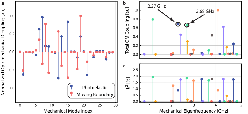
Figure S1: Optomechanical coupling simulations. a Simulated normalized photoelastic and moving boundary optomechanical coupling to the fundamental TE optical mode for the first $30$ mechanical breathing modes. b Total optomechanical coupling for the first $30$ mechanical breathing modes to the fundamental TE optical mode plotted as a function of the mechanical modes’ eigenfrequencies. c Plot of the electromechanical coupling coefficient, $k^{2}$, as a function of the mechanical modes’ eigenfrequencies. Colors are cycled for ease of comparison with the plot in b.

We also calculate the electromechanical coupling coefficient $k^{2}$ for each mechanical mode by performing FEM simulations, in which the electrodes of the device are driven with an oscillating voltage. From these simulations we extract the device’s series resonance frequency, $\omega_{s}$, and parallel resonance frequency, $\omega_{p}$, associated with each of the mechanical modes simulated in Fig. S1a [2]. We then obtain the coupling coefficient from

$$k^{2}=\frac{\omega_{p}^{2}-\omega_{s}^{2}}{\omega_{p}^{2}}.$$ (S13)

The values of $k^{2}$ are plotted in Fig. S1c along the same frequency axis as the values of optomechanical coupling in Fig. S1b. In general, modes with significant optomechanical coupling also have nonzero $k^{2}$. This is because the same mechanical mode symmetries that allow for the integrals of equations (S9) and (S10) to be nonzero enable the electric field driven by the device’s electrodes to effectively overlap with the piezoelectrically generated electric field associated with the mechanical mode. We find that the simulated mode at $2.68\text{\,}\mathrm{GHz}$ labeled in black in Fig. S1b has both high optomechanical and electromechanical coupling. Yet, experimentally we find the mode at $2.31\text{\,}\mathrm{GHz}$, which we believe corresponds to the simulated mode at $2.27\text{\,}\mathrm{GHz}$, produces the most efficient modulation. This discrepancy and similar inconsistencies can be explained by the much larger quality factor we measure for the $2.31\text{\,}\mathrm{GHz}$ resonance (see S-IIIc for quality factor details).

S-III: Measurement Techniques.

S-IIIa: Calculation of Intensity Signal. Consider that the optical signal from the chip in the upper arm of the interferometer and entering the photodetector of Fig. 2c has the form $E_{u}(t)=A_{u}\exp\left\{i\left[-\omega t+\alpha\sin\left(\Omega t\right)\right]\right\}$, and similarly that of the lower arm has the form $E_{l}(t)=A_{l}\exp\left\{i\left[-\left(\omega+\Delta\right)t-\phi\right]\right\}$, where $A_{u}$ and $A_{l}$ are the real-valued amplitudes of the fields in the upper and lower arm, respectively, $\omega$ is the laser angular frequency, $\alpha$ is the modulation depth, $\Omega$ is the angular frequency of the microwave drive, $\Delta$ is angular frequency shift imparted by the commercial AOFS, and $\phi$ is the static phase-difference between the two fields due to the unbalanced state of the interferometer, which also accounts for the phases imparted by the 2x2 fiber directional couplers. We assume that each frequency component generated by the phase-modulation process is subject to the same transmission coefficient associated with the various components in the measurement setup, including the grating couplers, fiber directional couplers, and any Fabry-Perot cavities formed between chip or fiber facets. Since the modulation depths considered here are small enough that the vast majority of the optical power will remain within the first few sidebands, the assumption is valid barring the presence of any extremely dispersive or frequency selective elements. With this we can write the intensity signal incident on the fast photodetector as

$$I(t) =\left[E_{u}(t)+E_{l}(t)\right]\left[E_{u}^{*}(t)+E_{l}^{*}(t)\right]\vphantom{\left\{\sum_{n=-\infty}^{\infty}\right\}}$$ (S14)

$$I(t) =A_{u}^{2}+A_{l}^{2}+A_{l}A_{u}\left\{\exp\left\{i\left[\Delta t+\alpha\sin\left(\Omega t\right)+\phi\right]\right\}+\exp\left\{-i\left[\Delta t-\alpha\sin\left(-\Omega t\right)+\phi\right]\right\}\right\}\vphantom{\left\{\sum_{n=-\infty}^{\infty}\right\}}$$ (S15)

$$I(t) =A_{u}^{2}+A_{l}^{2}+A_{l}A_{u}\left\{\exp\left[i\left(\Delta t+\phi\right)\right]\sum_{n=-\infty}^{\infty}J_{n}(\alpha)\exp\left(in\Omega t\right)+\exp\left[-i\left(\Delta t+\phi\right)\right]\sum_{n=-\infty}^{\infty}J_{n}(-\alpha)\exp\left(in\Omega t\right)\right\}$$ (S16)

$$I(t) =A_{u}^{2}+A_{l}^{2}+A_{l}A_{u}\left\{\sum_{n=-\infty}^{\infty}J_{n}(\alpha)\exp\left\{i\left[\left(n\Omega+\Delta\right)t+\phi\right]\right\}+\sum_{n=-\infty}^{\infty}J_{n}(\alpha)\exp\left\{-i\left[\left(n\Omega+\Delta\right)t+\phi\right]\right\}\right\}$$ (S17)

$$I(t) =A_{u}^{2}+A_{l}^{2}+2A_{l}A_{u}\sum_{n=-\infty}^{\infty}J_{n}(\alpha)\cos\left[\left(n\Omega+\Delta\right)t+\phi\right].\vphantom{\left\{\sum_{n=-\infty}^{\infty}\right\}}$$ (S18)

We can see that the intensity signal consists of a constant term and a sum of terms weighted by Bessel functions that each oscillate at a distinct frequency, $n\Omega+\Delta$. In order to elucidate the importance of the AOFS in the lower arm, we will now derive the intensity $I^{\prime}$ in the case that $\Delta\rightarrow 0$; i.e. when there is no AOFS. We have that

$$I^{\prime}(t) =A_{u}^{2}+A_{l}^{2}+2A_{l}A_{u}\sum_{n=-\infty}^{\infty}J_{n}(\alpha)\cos\left(n\Omega t+\phi\right).\vphantom{\left\{\sum_{n=-\infty}^{\infty}\right\}}$$ (S19)

$$I^{\prime}(t) =A_{u}^{2}+A_{l}^{2}+2A_{l}A_{u}\left[\cos\left(\phi\right)\sum_{n=-\infty}^{\infty}J_{n}(\alpha)\cos\left(n\Omega t\right)-\sin\left(\phi\right)\sum_{n=-\infty}^{\infty}J_{n}(\alpha)\sin\left(n\Omega t\right)\right]$$ (S20)

$$I^{\prime}(t) =A_{u}^{2}+A_{l}^{2}+4A_{l}A_{u}\left\{\cos\left(\phi\right)\sum_{n=0}^{\infty}J_{2n}(\alpha)\cos\left(2n\Omega t\right)+\sin\left(\phi\right)\sum_{n=1}^{\infty}J_{2n-1}(\alpha)\sin\left[\left(2n-1\right)\Omega t\right]\right\}$$ (S21)

$$I^{\prime}(t) =A_{u}^{2}+A_{l}^{2}+2A_{l}A_{u}J_{0}(\alpha)\cos(\phi)+4A_{l}A_{u}\left\{\cos\left(\phi\right)\sum_{n=1}^{\infty}J_{2n}(\alpha)\cos\left(2n\Omega t\right)+\sin\left(\phi\right)\sum_{n=1}^{\infty}J_{2n-1}(\alpha)\sin\left[\left(2n-1\right)\Omega t\right]\right\},$$ (S22)

where we have made use of a trigonometric identity and the fact that for even $n$, $J_{n}(\alpha)=J_{-n}(\alpha)$, while for odd $n$, $J_{n}(\alpha)=-J_{-n}(\alpha)$. One salient difference between $I(t)$ and $I^{\prime}(t)$ is for the former the static phase difference $\phi$ uniformly shifts the phase of the oscillating sinusoids, while for the latter it modulates the intensity of the even and odd harmonics of $\Omega$ present at the photodetector. Thus, if there are any phase fluctuations in the fiber causing $\phi\rightarrow\phi(t)$ to become a random function of time, the readout of the strength of the intensities at the various frequencies $n\Omega$ will vary randomly in time; what is worse, since the intensities are modulated by $\cos\phi$ and $\sin\phi$, the average intensity of any given sideband will be zero given $\phi(t)$ covers a whole cycle of phase. The presence of the AOFS removes the issue of noise in the strength of the oscillating intensity terms and eliminates the need to phase-lock the interferometer. Also, we can see that $I^{\prime}(t)$ does not distinguish between $n$ and $-n$, whereas $I(t)$ maps them to distinct frequencies whose Fourier decomposition may be extracted by a spectrum analyzer. Although a pure phase-modulation process generates symmetric power conversion to the red and blue-shifted sidebands, the ability to distinguish them allows us to identify the presence of other processes such as deliterious frequency-discriminating Fabry-Perot cavities formed between fiber and waveguide facets or intermodal Brillouin scattering.

S-IIIb: Determination of modulation depth. The photodetector in our setup outputs the signal mathematically represented in equation (S18). We obtain the RF power $P_{n}$ at a given frequency $n\Omega+\Delta$ by passing this signal to a radio frequency spectrum analyzer (RFSA). For each $n$, these powers are proportional to $J_{n}^{2}(\alpha)$ with the same constant of proportionality, so $R_{nm}\overset{\text{def}}{=}P_{n}/P_{m}=J_{n}^{2}(\alpha)/J_{m}^{2}(\alpha)$. Since $R_{mn}$ is a value directly measured from the RFSA, and $J_{n}$ and $J_{m}$ are known functions, we can find a modulation depth $\alpha$ that satisfies this equation. To confirm the validity of these extracted modulation depths, we calculated and compared the $\alpha$ measured from several different sideband ratios $R_{mn}$. Fig. S2 shows the measured $\alpha$ from five different sideband ratios as a function of driving voltage for the device reported in the main text, and we observe close agreement amongst them. For modulation depths calculated from ratios with higher order sidebands (e.g. $R_{40}$) the power signal on the RFSA does not emerge from the noise floor until a certain cutoff voltage, and the essentially random modulation depth measurements until that point are excluded from the plots.

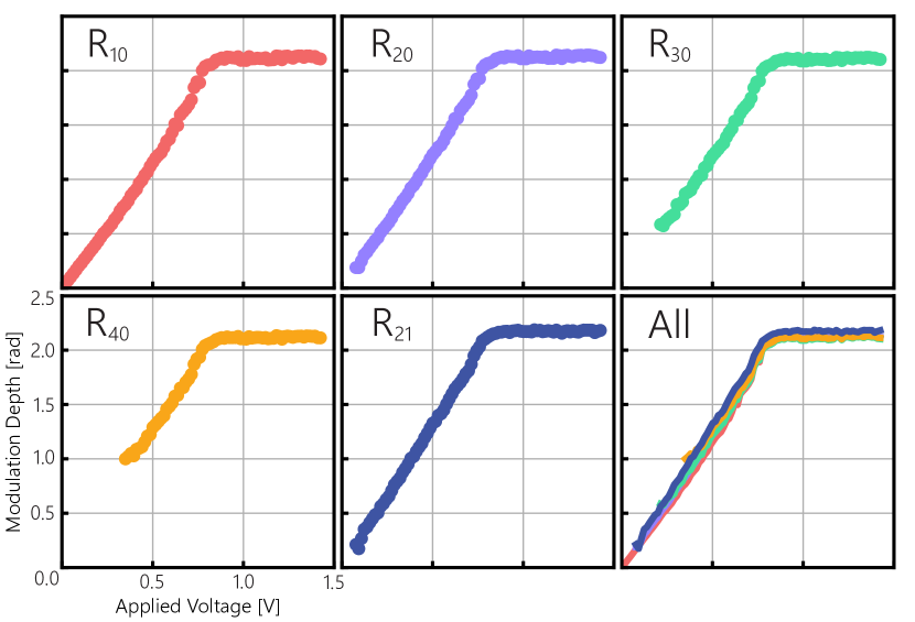
Figure S2: Comparison of measured modulation depths. Modulation depths extracted from five different sideband power ratios $R_{mn}$. Driving voltage was swept at a fixed frequency of $2.31\text{\,}\mathrm{GHz}$, and the axes for each subplot are the same.

S-IIIc: Determination of Mechanical Quality Factors. We extract the mechanical quality factors of the observed mechanical modes from modulation depth versus frequency data. The photoelastic and moving-boundary perturbations to the optical mode’s effective refractive index are proportional to the mechanical strain magnitude. Thus, the device’s modulation depth is also proportional to the strain magnitude. Around nearly every frequency at which we observe resonant modulation, we find doublet mechanical resonances. Because the device has discrete translational symmetry from the periodic nanopillar supports, it behaves as a weak phononic crystal, which gives rise to the doublets.

We numerically fit the measured modulation depth data $\alpha(\Omega)$ to a sum of Lorentzian functions of the form

$$\tilde{\alpha}(\Omega)=\sum\limits_{j}A_{j}\frac{\left(\Omega_{0,j}/2Q_{j}\right)^{2}}{\left(\Omega-\Omega_{0,j}\right)^{2}+\left(\Omega_{0,j}/2Q_{j}\right)^{2}},$$ (S23)

where $\Omega_{0,j}$ is $j$th resonance angular frequency, $A_{j}$ is the $j$th Lorentzian amplitude in units of radians, and $Q_{j}$ is the $j$th mechanical quality factor. The fitted parameters are listed in Fig. S3a and plotted in Fig. S3b-d. Fits are obtained from batches of data within the neighborhood of observed resonances. For the frequency range around $2.31\text{\,}\mathrm{GHz}$, we fit a sum of four Lorentzians (Fig. S3d) because two pairs of doublets existed within each other’s bandwidths. For the resonance with central frequency $3.34\text{\,}\mathrm{GHz}$, we fit a single Lorentzian because no doublet-feature was observed. All other Lorentzians were fit in pairs, and parameters that were simultaneously extracted from the same batch of data are grouped by color in Fig. S3a.

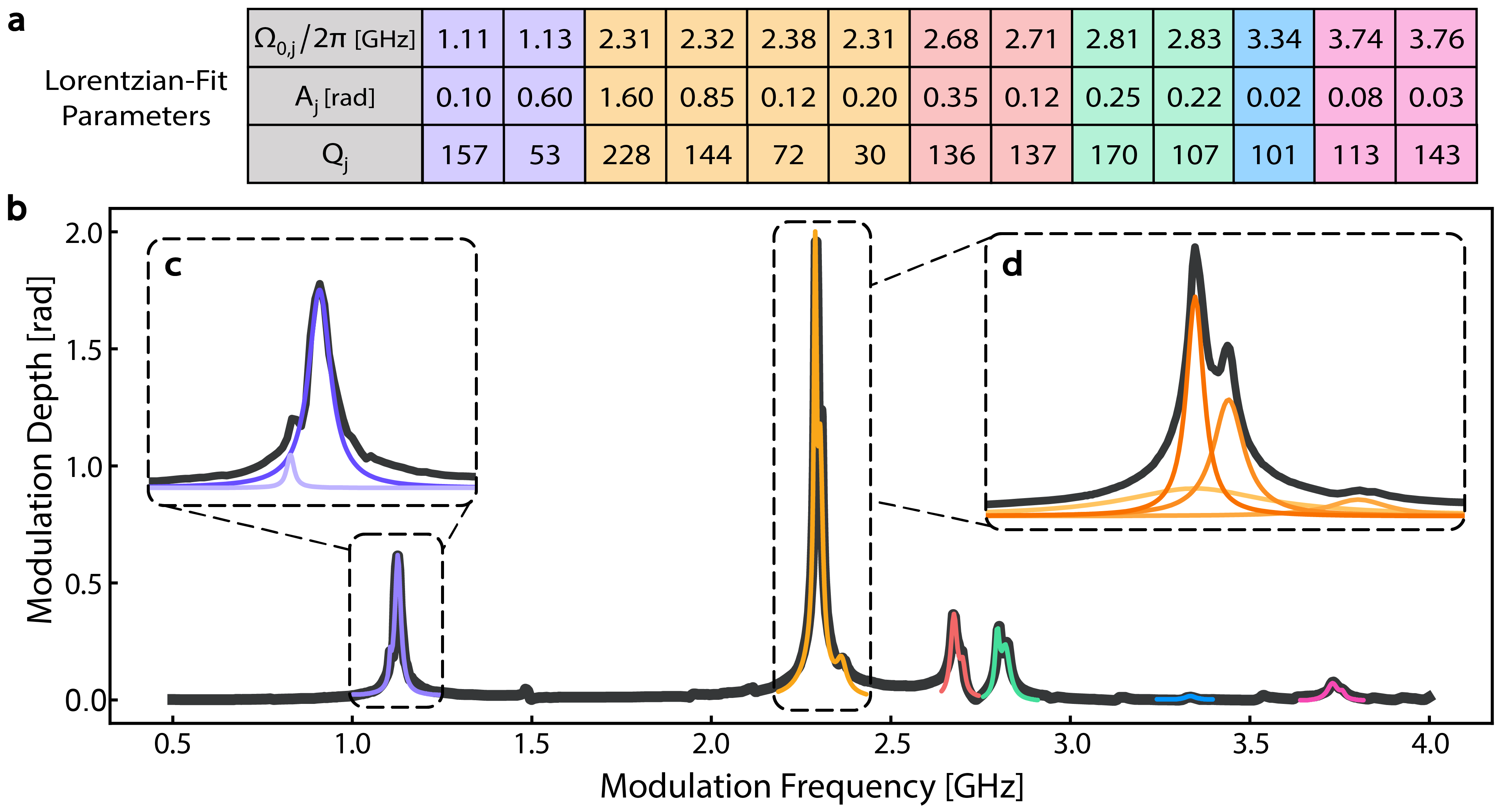
Figure S3: Determination of mechanical quality factors. a Lorentzian fit parameters including the central frequencies ($\Omega_{0,j}/2\pi$), amplitudes $A_{j}$, and quality factors $Q_{j}$ for each resonance. Colors correspond to parameters fit from the same batch of data. b Plot of the numerical fits (in color) superimposed on the measured modulation depth (in gray). Insets show in c the Lorentzian doublet fit around $1.1\text{\,}\mathrm{GHz}$ and in d the Lorentzian quadruplet fit around $2.3\text{\,}\mathrm{GHz}$.

S-IV: Simulation of Broadband Operation

We simulate the optical bandwidth of our modulator by calculating the photoelastic and moving boundary coupling of equations (S9) and (S10), respectively, as a function of optical wavelength. We do so by performing FEM simulations of the structure from the main text for wavelengths spanning from $300\text{\,}\mathrm{nm}$ to $1000\text{\,}\mathrm{nm}$ in increments of $20\text{\,}\mathrm{nm}$. At a fixed optical wavelength, the group velocity parameter in the coupling equations does not play a role in the comparison of optomechanical coupling from distinct mechanical modes. Here, we are comparing coupling across wavelengths, so we calculate it from the simulations and plot it along with the mode’s phase velocity in Fig. S4a. We expectedly observe that the optical mode profile becomes decreasingly confined as wavelength is increased (Fig. S4b-d). If the sign of the mechanical strain field changes sign near the SiN_x-SiO₂ boundary, a lack of confinement causes the mode to sample both negative and positive changes to refractive index, thereby decreasing the photoelastic coupling integral. Likewise, if the strain-field maintains the same sign near the waveguide boundary, decreased confinement can lead to increased photoelastic coupling. Moving boundary coupling is modified by the degree to which the optical mode is concentrated at the SiN_x-SiO₂ boundary, which is affected by the confinement of the mode. Despite the photoelastic and moving boundary effects having the above dependencies on wavelength, we expect the overall coupling to remain relatively constant over wavelength ranges spanning hundreds of nanometers because the modal profile varies slowly with respect to wavelength.

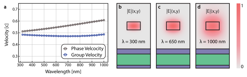
Figure S4: Optical mode as a function of wavelength. a Plot of group velocity and phase velocity in units of the free-space speed of light for the device’s optical waveguide as a function of free-space wavelength. b-d Plots of the electric field norm for the fundamental transverse electric mode at $300\text{\,}\mathrm{nm}$, $650\text{\,}\mathrm{nm}$, and $1000\text{\,}\mathrm{nm}$. The simulations from which these are derived include a large domain of air surrounding the waveguide to ensure the expanding optical mode does not interact with nonphysical boundary conditions.

Since predictions for modulation efficiencies calculated from simulated optomechanical coupling do not account for mechanical quality factor or device impedance, we calibrate out prediction from our experimental results. From the experimentally obtained data, we have the frequencies at which mechanical resonances occur and the modulation depth $\alpha_{0}^{(j)}$ the $j$th mode imparts at $\lambda_{0}=$730\text{\,}\mathrm{nm}$$. By combining this information with simulations of the perturbation to the propagation constant $\Delta\beta^{(j)}(\lambda)$ imparted by the $j$th mechanical to the optical mode with free-space wavelength $\lambda$, we obtain a prediction for the modulation depth $\alpha(\lambda)$. We have that

$$\frac{\alpha^{(j)}(\lambda)}{\alpha^{(j)}_{0}}=\Delta\beta^{(j)}(\lambda)L\cdot\frac{1}{\Delta\beta^{(j)}(\lambda_{0})L}=\frac{\Delta\beta^{(j)}(\lambda)}{\Delta\beta^{(j)}(\lambda_{0})}\overset{\text{def}}{=}R^{(j)}(\lambda),$$ (S24)

where $L$ is the length of the device. Thus, for the $j$th mechanical mode and some optical wavelength $\lambda$, we can predict the device’s modulation depth to be $\alpha^{(j)}(\lambda)=R^{(j)}(\lambda)\alpha^{(j)}_{0}$. This calibration of the simulated prediction to the experimentally measured values at $730\text{\,}\mathrm{nm}$ has the effects of electromechanical coupling, mechanical quality factor, and microwave reflection baked into the values. Fig. S5c shows these simulated modulation depths for three selected mechanical modes over the transparency window of the SiN_x waveguide. From this, we can see that the modulator would function well over an optical bandwidth spanning hundreds of nanometers. As wavelength is decreased, the optical mode’s rate of phase accumulation inherently increases because of the increase to its propagation constant. If $\Delta\beta^{(j)}(\lambda)$ is relatively constant as a function of wavelength, this increase in modulation depth toward shorter wavelengths is observed (e.g. for modes 2 and 3 in Fig. S5c). However, for Mode 1 the optomechanical coupling strength decreases as a function of optical wavelength and counteracts the effect of increasing propagation constant, rendering its modulation depth nearly constant over the simulated wavelength range.

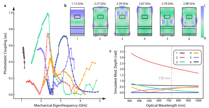
Figure S5: Simulated broadband operation of the phase-modulator. a Plot of normalized photoelastic optomechanical coupling against eigenfrequency for six mechanical resonances which are simulated as the device width varies from $600\text{\,}\mathrm{nm}$ to $2.3\text{\,}\mathrm{\SIUnitSymbolMicro m}$. b The mechanical displacement profiles and eigenfrequencies of the six mechanical modes at a device width of $w_{1}=$1.25\text{\,}\mathrm{\SIUnitSymbolMicro m}$$. c Plot showing simulated modulated depth as a function of optical wavelength for the same six mechanical modes as in a. The simulated drive power was $15\text{\,}\mathrm{mW}$, and the modulation depths are calibrated to the experimentally measured values at $730\text{\,}\mathrm{nm}$.

For the Raman control of hyperfine qubits, our device must be capable of producing resonantly enhanced phase modulation at frequencies specific to commonly utilized neutral atoms and trapped ions. To study this, we simulated the optical and mechanical modes of our device as the width ($w_{1}$ of Fig. 1a in the main text) was swept from from $600\text{\,}\mathrm{nm}$ to $2.3\text{\,}\mathrm{\SIUnitSymbolMicro m}$. We then calculated the photoelastic optomechanical coupling for each mechanical mode to the fundamental transverse electric optical mode as a function of device width. We present the result of this calculation for six mechanical breathing mode families (Fig. S5b), where we have mapped the device-width parameter to the resonance frequency of the mechanical modes. Generally, as the device is made increasingly narrow, the resonance frequency for a given mechanical mode increases. However, for modes such as mode 3 that have strain almost entirely along the vertical axis, the resonance frequency hardly depends at all upon the device’s width. We find that over frequencies ranging from $1\text{\,}\mathrm{GHz}$ to $5\text{\,}\mathrm{GHz}$, one can always find a mechanical mode exhibiting optomechanical coupling comparable to that of the device presented in the main text. In principle, one could achieve higher frequency operation by narrowing the device beyond $600\text{\,}\mathrm{nm}$, however difficulties with fabrication likely preclude this for now. At each simulated device width, we do not re-optimize the waveguide core width because this is computationally expensive and modifies the mechanical resonance frequencies. However, if one were targeting a specific frequency, the core width could also be varied to achieve even higher coupling.

References

- [1] Steven G. Johnson, M. Ibanescu, M. A. Skorobogatiy, O. Weisberg, J. D. Joannopoulos, and Y. Fink. Perturbation theory for Maxwell’s equations with shifting material boundaries. Physical Review E, 65(6):066611, June 2002.
- [2] Jose Luis Sanchez-Rojas, editor. Piezoelectric Transducers. MDPI - Multidisciplinary Digital Publishing Institute, August 2020.
- [3] Ryan Patrick Scott. Design and Applications of Resonant Electro-Optic Time Lenses. PhD thesis, University of California Los Angeles, 1995.
- [4] Hao Tian, Junqiu Liu, Alaina Attanasio, Anat Siddharth, Terence Blésin, Rui Ning Wang, Andrey Voloshin, Grigory Lihachev, Johann Riemensberger, Scott E. Kenning, Yu Tian, Tzu Han Chang, Andrea Bancora, Viacheslav Snigirev, Vladimir Shadymov, Tobias J. Kippenberg, and Sunil A. Bhave. Piezoelectric actuation for integrated photonics. Advances in Optics and Photonics, 16(4):749–867, December 2024. Publisher: Optica Publishing Group.
- [5] Gustavo S. Wiederhecker, Paulo Dainese, and Thiago P. Mayer Alegre. Brillouin optomechanics in nanophotonic structures. APL Photonics, 4(7):071101, July 2019.