Energy-as-a-Service for RF-Powered IoE Networks: A Percolation Theory Approach
Abstract
Due to the involved massive number of devices, radio frequency (RF) energy harvesting is indispensable to realize the foreseen Internet-of-Everything (IoE) within 6G networks. Analogous to the cellular networks concept, shared energy stations (ESs) are foreseen to supply energy-as-a-service (EaaS) in order to recharge devices that belong to different IoE operators who are offering diverse use cases. Considering the capital expenditure (CAPEX) for ES deployment along with their finite wireless energy transfer (WET) zones, spatial energy gaps are plausible. Furthermore, the ESs deployment cannot cover of the energy-harvesting devices of all coexisting IoE use cases. In this context, we utilize percolation theory to characterize the feasibility of large-scale device-to-device (D2D) connectivity of IoE networks operating under EaaS platforms. Assuming that ESs and IoE devices follow independent Poisson point processes (PPPs), we construct a connectivity graph for the IoE devices that are within the WET zones of ESs. Continuum percolation on the construct graph is utilized to derive necessary and sufficient conditions for large-scale RF-powered D2D connectivity in terms of the required IoE device density and communication range along with the required ESs density and WET zone size. Fixing the IoE network parameters along with the size of WET zones, we obtain the approximate critical value of the ES density that ensures large-scale connectivity using the inner-city and Gilbert disk models. By imitating the bounds and combining the approximations, we construct an approximate expression for the critical ES density function, which is necessary to minimize the EaaS CAPEX under the IoE connectivity constraint.
Index Terms:
Energy-as-a-Service (EaaS), Internet of Everything (IoE), stochastic geometry, percolation theory, Gilbert disk model.I Introduction
In the 6G era, wireless connectivity is foreseen to be global, ubiquitous, and massive. In addition to transforming every object in our life into an intelligent and connected device, the proliferating 6G Internet of Everything (IoE) use cases (e.g., digital twins, ubiquitous environmental monitoring, precision agriculture, smart cities, wearable devices, etc.) will bring massive numbers of additional wireless devices [1, 2, 3]. In such a massive network setup, monitoring and replacing/recharging the batteries of the devices is an overwhelming process that imposes high operational expenditure (OPEX). Such high OPEX can be alleviated by utilizing wireless energy transfer (WET) along with energy-harvesting (EH) technologies [4, 5, 6, 7]. In particular, energy providers deploy energy stations (ESs) for WET, which offers energy-as-a-service (EaaS) to IoE operators/consumers who equip their devices with EH modules. The range of far-field wireless charging can reach tens of meters to meet the charging requirements of most mobile application scenarios. Also, the use of green energy can flexibly provide free and continuous electromagnetic energy for ESs [2, 3]. The proliferating IoE use cases make such energy services a worthwhile business opportunity [8]. In fact, the EaaS platform is considered an attractive business model that is estimated to exceed billion annual global market value by 2026 [9]. In the future, such EaaS platforms can not only serve mobile users and sensor networks on the ground, but also provide wireless power support for unmanned aerial vehicles (UAVs) and more near space platforms [10].
To reduce CAPEX, EaaS operators strive to satisfy the IoE energy demand with minimal ESs deployment. Assuming that IoE operators/consumers mandate large-scale D2D connectivity of their devices,111D2D connectivity can reflect the maximum communication range of each device, and hence, large-scale connectivity enables long-range information dissemination. D2D connectivity can also be interpreted as the maximum sensing range of each device, and hence, large-scale connectivity is important for monitoring and intrusion detection IoE use cases. graph and percolation theories are best suited to estimate the necessary and sufficient ES deployments that satisfy the IoE operators/consumers connectivity demand. In particular, graph theory provides a tractable mathematical representation for the interactions among network components, where vertices are used to model devices and edges represent direct relationships among vertices [11, 12]. Percolation theory is used to characterize the large-scale connectivity of graphs. Since D2D connectivity and WET zone coverage depend on the relative locations of IoE devices with respect to each other and with respect to ESs, random geometric graphs (RGGs) are utilized [13]. Assuming that ESs and IoE devices follow independent Poisson point processes (PPPs), a WET-aware connectivity (WC)-RGG for the IoE devices is constructed based on their relative locations, D2D communication range, and WET zone coverage. Using continuum percolation on the IoE WC-RGG, we characterize the network parameters that enable large-scale D2D connectivity of the IoE network. Hence, helping operators estimate the required CAPEX to deliver a successful EaaS.
I-A Related Work
In this paper, we propose to apply the EaaS platform to support large-scale D2D communications between RF-powered IoE devices. Using percolation theory, we prove the feasibility of such an EaaS platform and help operators estimate critical ES density, further, the required CAPEX. Therefore, we divide the related work into: i) percolation theory for wireless networks and ii) stochastic geometry for RF-powered wireless networks.
Percolation theory for wireless networks: Continuum percolation on RGGs has been widely utilized to study the large-scale network-wide performance of wireless networks with randomly located devices [13, 14, 15]. For instance, the authors in [16] utilized continuum percolation to quantify the impact of aggregate network interference on large-scale network connectivity. End-to-end capacity in large-scale networks was characterized in [17] via percolation theory. Using the concept of information secrecy, the authors in [18, 19] found the relative densities of legitimate devices and eavesdroppers that enable large-scale private message dissemination among legitimate devices. In cognitive radio networks, the authors in [20, 21, 22] characterized the relationship between the intensity of secondary devices and primary devices to allow large-scale connectivity of the secondary network. Simultaneous large-scale connectivity of both the primary and secondary devices in cognitive networks was studied in [23]. For sensing/monitoring applications, the path exposure problem was characterized in [24, 25], where the authors found the critical density of sensors/cameras to detect moving objects over arbitrary paths through a given region. In the context of cyber-security, the authors in [26] utilized continuum percolation to quantify the required spatial firewalls to thwart large-scale outbreaks of malware worms in wireless networks. By investigating the BS networks assisted by reconfigurable intelligent surfaces (RISs), authors in [27] derived the lower bound of the critical density of RISs. In [28], based on dynamic bond percolation, authors proposed an evolution model to characterize the reliable topology evolution affected by the nodes and links states. However, WET-enabled large-scale connectivity of RF-powered IoE networks is still an open problem.
Stochastic geometry for
RF-powered wireless networks: RF-powered wireless communication has been extensively studied at the link-level performance as summarized in [29]. In large-scale RF-powered networks, stochastic geometry was utilized to provide spatial averages of link-level performance metrics such as coverage probability, rate, or delay. For instance, the work in [30, 31] characterized the energy efficiency for PPP downlink cellular networks that are powered via renewable energy sources. Outage probability and rate of downlink simultaneous wireless information and power transfer (SWIPT) were studied in [32] for cooperative non-orthogonal multiple access (NOMA) and in [33] for cell-free massive multiple-input multiple-output (MIMO) networks. On the uplink side, the work in [34] characterized coverage probability with channel inversion power control. Delay and packet throughput for grant-free uplink access of RF-powered Internet of Things (IoT) was characterized in [35]. Outage probability and self-sustainability of D2D RF-powered IoT networks were characterized in [36, 37, 38]. End-to-end outage probability for RF-powered D2D decode-and-forward relaying was studied in [39]. D2D-enabled proactive caching for RF-powered wireless networks was studied in [40]. For non-terrestrial networks, the authors in [41] optimized the altitude of RF-powered aerial base stations serving terrestrial devices. A similar scenario was studied in [42] for laser-powered aerial base stations. Authors in [43] combined the backscatter communication with RF-powered cognitive networks, and investigated the resource allocation for channel selection and backscatter power allocation. In [44], authors evaluated the effect on RF-powered IoT network performance of RIS density, RIS reflecting element number, and charging stage ratio. However, none of the aforementioned stochastic geometry frameworks can be utilized to study network-wide connectivity of RF-powered IoE networks in order to help EaaS providers estimate the required intensity of ESs.
I-B Contributions
As an important performance metric of IoE networks, connectivity has its unique value. It refers to the ability to generate remote multi-hop D2D transmission links, which further promotes the flexibility and reliability of the IoE networks. Higher network-wide connectivity of IoE networks not only helps realize more functions in different applications, but also helps achieve better performance, such as higher detection accuracy, stronger fault tolerance, and stronger noise immunity et al. However, to the best of the authors’ knowledge, there are no available network-wide connectivity studies for RF-powered wireless networks, which is foundational to estimating the CAPEX for EaaS providers. This paper covers such a gap with the following set of contributions:
-
•
We develop a novel WC-RGG, and utilize continuum percolation, to study large-scale multi-hop D2D connectivity in RF-powered IoE networks.
-
•
We prove the existence of a finite critical density of ESs that enable network-wide connectivity of battery-less IoE devices.
-
•
We obtain an accurate approximate expression for critical ES density as a function of IoE device density, IoE D2D communication range, and ES WET zone sizes, which is important to estimate the CAPEX of EaaS.
-
•
Our analysis provides an alternative way to compute the well-celebrated approximate percolation critical density for PPP networks with unit-length connectivity radius as , which further validates our analysis.
Organization: The organization of the paper is as follows. The system model and assumptions are detailed in Sec.II. Sec.III proves the feasibility of large-scale connectivity of RF-powered IoE networks under EaaS platforms. Sec.V provides useful approximations for the critical density of ESs, which give insights into the CAPEX of EaaS. Numerical and simulation results are discussed in Sec.V before the paper is concluded in Sec.VI.
Notations: In this paper, we utilize the following set of notations. The probability of an event is denoted as . The right arrow means the event on the left of it causes events on the right side. The main symbols used in this paper are summarized in Table.I.
| Notation | Description |
|---|---|
| ; ; | The set of locations of IoE devices; the density of IoE devices; the maximum communication range |
| ; ; | The set of locations of ESs; the density of ESs; the maximum charging/energy supporting range |
| The RGG representation of active IoE devices with vertex set and edge set | |
| The probability of percolation in when | |
| The probability of percolation in when | |
| ; ; ; | The hexagonal lattice, randomly selected hexagon, side length of a hexagon and outer envelope in sub-critical regime |
| ; ; ; | The hexagonal lattice, randomly selected hexagon, side length of a hexagon and inner envelope in super-critical regime |
| ; ; | The connected component in , and |
| ; ; | The critical ES density and its lower bound and upper bound |
| ; ; | The approximations using the Inner-city model, a simple Gilbert model or combining them together |
II System Model
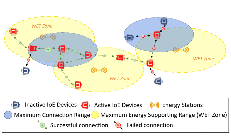
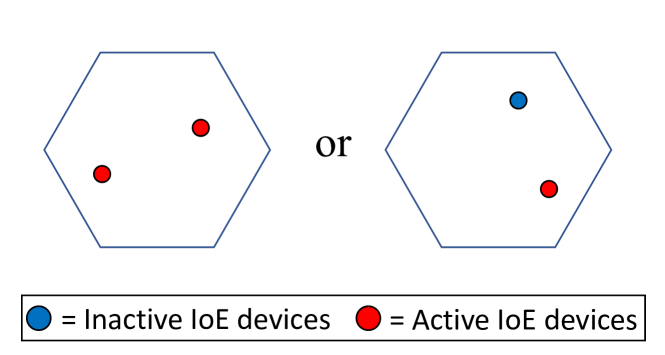
We consider an IoE network with battery-less devices that are spatially scattered according to a PPP with density . The IoE devices are equipped with EH modules that are powered through an EaaS operator with ESs that are deployed according to an independent PPP with density . The independence between and is justified by the fact that an EaaS operator is serving many IoE networks, and hence, the ES deployment is not customized to any of them. Instead, the EaaS operators deploy their ESs in strategic locations where there is high demand from several IoE network operators/consumers. The ESs have a maximum WET range (i.e., the maximum charging range for IoE devices), where each ES can provide EaaS to activate all IoE devices inside their WET zones. The IoE operators mandate a long-range network-wide D2D connectivity among their battery-less devices. In particular, the IoE operators seek an EaaS platform that is able to activate a sufficient number of devices that span the spatial domain and can reach each other through multi-hop D2D connections. Two battery-less IoE devices can establish a D2D connectivity if and only if they satisfy the following two conditions; i) each of the IoE devices falls within a WET zone of at least one ESs, and ii) both IoE devices are within the D2D communication range of from each other. A pictorial illustration of the RF-powered IoE operation under the EaaS platform is shown in Fig.1. Given the stringent power and complexity constraints of IoE devices, it is plausible to assume that , where each ES can support enough IoE devices and form a small IoE network around it. The transmit power of each ES should be much higher than the transmit power of each IoE device because the maximum distance between any ES and IoE devices in its WET zone should be larger than the distance between adjacent IoEs, and each ES is responsible for the energy supply of multiple IoE devices.
Following the aforementioned two connectivity conditions for battery-less devices, we construct a WC-RGG for RF-powered IoE networks operating under an EaaS platform. The WC-RGG is denoted as , where is the set of vertices defined as:
| (1) |
and is the set of edges given by:
| (2) |
Large-scale network-wide connectivity of the RF-powered IoE can be characterized via continuum percolation over the WC-RGG.222It is important to mention that continuum percolation does not guarantee full connectivity of the WC-RGG. Instead, continuum percolation guarantees that there exists a large number of vertices within the WC-RGG that span the spatial domain and can reach each other through multi-hop connections. We first define a component , as a connected sub-graph where any two vertices within are connected through a set of consecutive edges in . The non-zero percolation is an event where there exists an infinite-size connected component within the WC-RGG with a non-zero probability. Without loss of generality, we assume that there is a device located at the origin that belongs to the connected component . The set cardinality of is denoted as and the percolation probability in is defined as:
| (3) |
To minimize the CAPEX of the EaaS operator and satisfy the large-scale D2D connectivity mandate of the IoE operator/consumer, the design objective for the ESs deployment can be formulated as:
| (4) |
The problem formulation in (4) seeks the minimum density of ESs that ensures large-scale D2D connectivity of the battery-less IoE networks. In the extreme case, when approaches , the ESs are dense enough to activate all IoE devices. Such a highly dense ES regime captures a scenario where there is no energy scarcity and is denoted hereafter by an infinity subscript to highlight that approaches . In the highly dense ES regime, the WC-RGG transforms to a conventional RGG with vertices and edges
| (5) |
In the highly dense ES regime, the percolation probability is only relevant to the IoE parameters and , which is given by:
| (6) |
Since the highly dense ESs regime transforms the WC-RGG to a conventional RGG of a PPP with density a connectivity range , the critical IoE parameters that ensure continuum percolation in such regime can be directly obtained from [45] as
| (7) |
where is the percolation critical density for a PPP RGG with unit-length connectivity radius.333It is worth noting that the exact value for is still an open problem. There are only known bounds and approximations for the critical density . It is worth noting that (7) is not only the sufficient condition for non-zero percolation when approaches , but also the necessary condition in RF-powered IoE networks where .
III Proof of concept
In this section, we define and prove the phase transition of the percolation probability for the WC-RGG (i.e., ). In particular, when the density of IoE devices satisfies the condition (7), there exists a critical ES density , below which remote multi-hop links can not be established and operates in the sub-critical regime. On the contrary, when the density of the ESs is above , then operates in the super-critical regime, where remote multi-hop links can be realized from the origin with a non-zero probability.
Following the percolation theory convention, we organize the proof into the following subsections. Sec.III-A presents the sub-critical regime for , which proves the need for enough ES density. We prove the sufficient condition for no percolation and derive the lower bound of . Sec.III-B presents the super-critical regime, in which we prove the sufficient condition for non-zero percolation and derive the upper bound of . Last but not least, Sec.III-C completes the proof of phase transition by showing the monotonicity of percolation probability in ES density . In Sec.III-C, we also derive the relationship between critical ES density and IoE device density, and define the critical ES density function.
III-A Sub-critical regime
This section proves that large-scale network-wide multi-hop links can not be realized when the ESs are not dense enough. In this case, the EaaS is not successful. We find the sufficient condition for no percolation and derive the lower bound of critical ES density . As a common practice in percolation theory, we study continuum percolation by mapping it to discrete lattices. Inspired by [26] and [46], we analyze the sub-critical regime by mapping the WC-RGG to a hexagonal lattice. We consider the special scenario where is the same as the side length of the hexagon such that two active IoE devices in two nonadjacent hexagons can not be connected via a direct D2D link.
Mapping to a Hexagonal Lattice in Sub-critical Regime: Let be a hexagonal lattice with a side and let be a randomly selected hexagon in the lattice. Hereafter, is denoted as a face in . Such a setup implies that is the minimum distance between IoE devices in two nonadjacent hexagons.
Definition 1 (Inactive face in sub-critical regime).
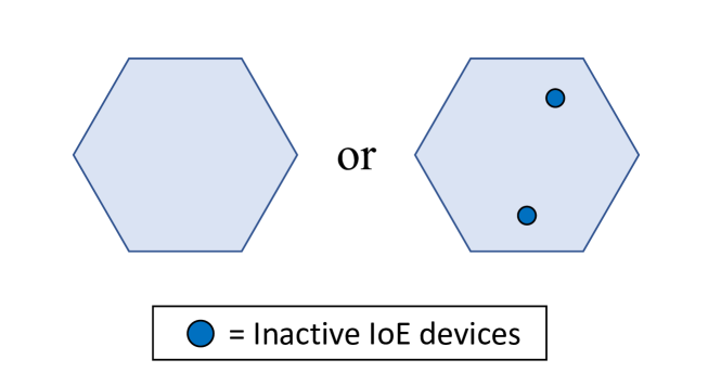
A face is denoted as inactive if it contains no edges of . As shown in Fig.2(a), the conditions to ensure that is an inactive face are: i) there is no IoE device in or ii) there is at least one IoE device but none of them are activated.
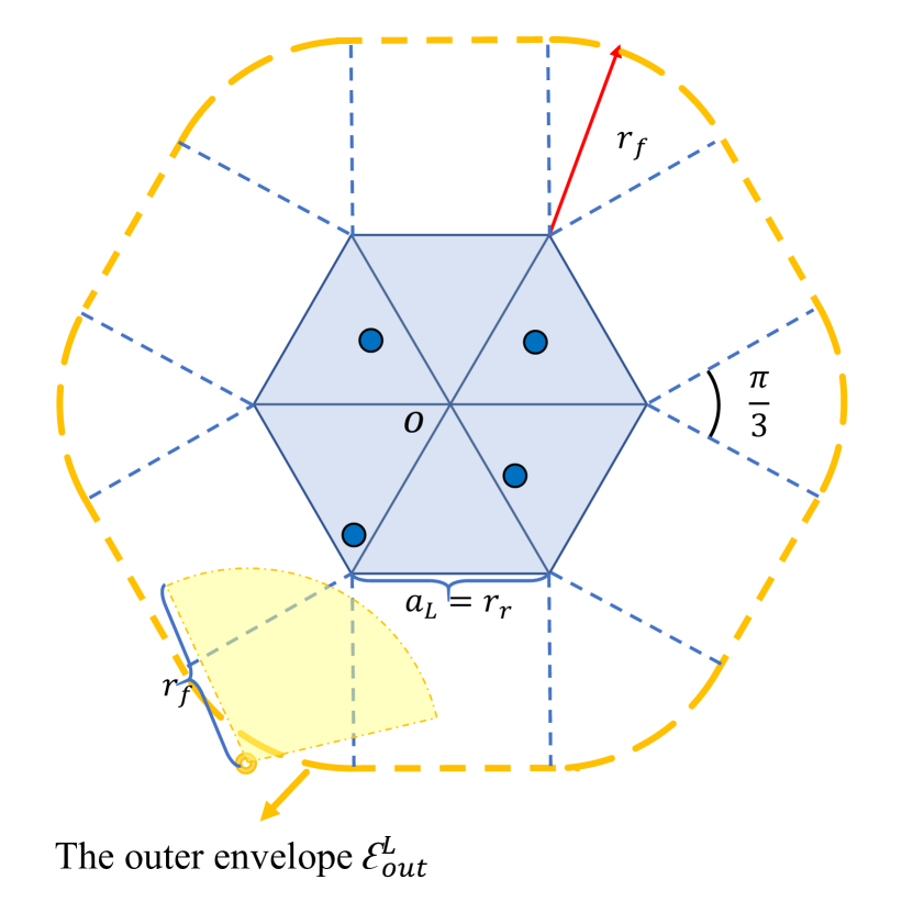
When there is no IoE device in , this face is inactive. We describe another extreme situation as shown in Fig.2(b). When one or more IoE devices are randomly distributed in but there is no ES inside the outer envelope , the devices located anywhere in can not be activated. Therefore, can not be activated as well. Considering these two cases, the probability satisfies:
| (8) |
where is the area of .
When , there exists a sequence of connected inactive faces which form an inactive path. The inactive path which starts and ends at the same face is defined as an inactive circuit as shown in Fig.2(c). We use to represent the inactive circuit around the origin. Then, the number of active faces around the origin is finite, i.e. . Because the side length of the hexagon , the devices inside can not be connected with those outside directly or indirectly. Then, the number of devices connected with the device at the origin is finite, i.e. . Based on this, we introduce the lower bound of critical ES density in Lemma 11.
Lemma 1 (Lower bound of critical ES density).
Mapping to the hexagonal lattice , the lower bound of critical ES density is
| (9) |
where
| (10) |
and
| (11) |
Proof:
See Appendix A. ∎
Remark 1.
Based on the lower bound in Lemma 11, we obtain the sufficient condition for no percolation (, ): i) or ii) . Because , , the sufficient condition for no percolation can be updated as: i) or ii) .
We can notice from (9) that as the density of IoE device approaches , the lower bound for the critical density of ESs approaches .
III-B Super-critical regime
This section proves that the probability of forming a giant connected component in the network is non-zero when ES density is dense enough. We also find the sufficient condition for non-zero percolation and derive the upper bound of critical ES density . Similar to the sub-critical regime, we analyze the super-critical regime by mapping the WC-RGG to a hexagonal lattice, however, with different dimensions.
Mapping to a Hexagonal Lattice in Super-critical Regime: Let be a hexagonal lattice with a side length of and let be a randomly selected hexagon (i.e., face) of . In this case, is the maximum distance between any two IoE devices in two adjacent hexagons, hence, all IoE devices in any two adjacent hexagons are able to connect.
Definition 2 (Active face in super-critical regime).
A face is denoted as active if it contains at least one IoE device that lies within a WET zone of any ES. As shown in Fig.3(a), to make be an active face, the sufficient condition is: i) there is one or more IoE devices and ii) at least one of them is activated.
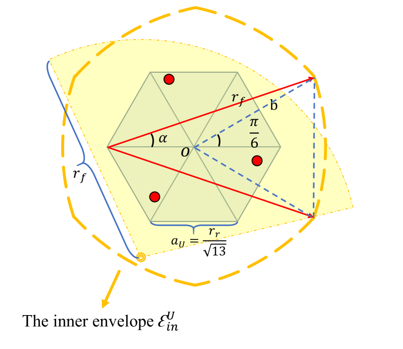
To derive an upper bound expression for the critical ES density, we consider the situation in Fig.3(b): there is at least one IoE device in and at least one ES inside the inner envelope . In this case, the hexagon is active because there is at least one active IoE device in . The probability satisfies:
| (12) |
where is the area of .
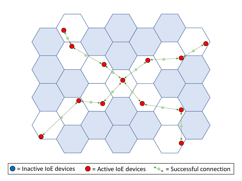
We also assume that there is an active IoE device at the origin. The face percolation happens in the hexagonal lattice when . An example of such a scenario is shown in Fig.3(c). At the same time, the number of IoE devices connected with the device at the origin is infinite, i.e. . Even if we overestimate the probability of an active face, it is available to analyze the super-critical regime. Based on this, we introduce the upper bound of critical ES density in Lemma 2.
Lemma 2 (Upper bound of critical ES density).
Mapping to the hexagonal lattice , the upper bound of critical ES density is
| (13) |
where
| (14) |
and
| (15) |
with and .
Proof:
See Appendix B ∎
Remark 2.
Based on the upper bound in Lemma 2, we obtain the sufficient condition for non-zero percolation (, ): i) and ii) . Because , this condition is sufficient enough.
We can notice from (13) that as the density of IoE device approaches , the upper bound of the critical density of ESs approaches .
III-C Critical ES density function
We have introduced the percolation probability in (4). To analyze the network-wide D2D connectivity in RF-powered IoE networks, it is important to find the critical ES density for the phase transition of the percolation probability. The phase transition is defined in Theorem 16.
Theorem 1 (Phase transition).
Let denote the percolation probability in the RGG , , there exists a critical value for the density of ESs such that
| (16) |
Proof:
We first prove that the percolation probability is a non-decreasing function of when . Consider two sets of ESs and with densities and , respectively, where . Since and are both PPPs, can be constructed by thinning with probability , thus . The set of active IoE devices is defined as for . Hence, for any . Considering the connected component with the IoE device at origin, obviously and . Therefore, indicates . That means the percolation probability is a non-decreasing function of .
In Remark 1 and Remark 2, we derive the sufficient conditions for no percolation and non-zero percolation. We know that for and for . As shown in (6), when , the percolation only depends on the density of IoE devices, i.e. . The sufficient condition for is , which means percolation probability is not always zero when increasing the value of , . Since is a non-decreasing function of , there should be a critical value which exhibits the phase transition shown in Theorem 16.
∎
To analyze the relationship between and , we introduce Lemma 18.
Lemma 3 (Critical ES density function).
The critical density of ESs is defined as a function written as , which is a non-increasing function of satisfying:
| (17) |
where
| (18) |
Proof:
When , the percolation probability is updated as . As a common conclusion in percolation theory, it is a non-decreasing function of . When and , . To prove Lemma 18, we consider two sets of IoE devices and with densities and , respectively, where . Since and are both PPPs, can be constructed by thinning with probability and . and are the connected component from active IoE devices in and , respectively. Therefore, and . Similar to the proof of Theorem 16, percolation probability is a non-decreasing function of . We define and . Then , while . Therefore, for .
When , because percolation probability is a non-decreasing function of and is the critical ES density of phase transition when . If we assume that for , is impossible because . So when , if , . This means that for the same value of , there is only a unique critical ES density, i.e. implies .
When , because percolation probability is a non-decreasing function of , . At the same time, because the percolation probability is also a non-decreasing function of and is the critical ES density. Thus, implies .
In conclusion, implies , and critical ES density is a non-decreasing function of .∎
IV Approximations
In the previous section, we discuss the sub-critical and super-critical regimes and complete the proof of phase transition of percolation probability in RF-powered IoE networks under an EaaS platform. We define the critical ES density as a function of IoE device density. In this section, we use some classic tools in graph theory, such as the inner-city model and Gilbert disk models, to introduce tight approximations for critical ES density function, which are important to estimate the ESs deployment CAPEX to offer a successful EaaS.
IV-A Inner City Model
When the density of IoE devices is not very large, the distribution of active IoE devices follows a special model denoted as the inner-city model, which is introduced in [13]. The inner-city model is generated from the complementary process of the Poisson hole process. In particular, the inner-city model is a Cox process with the intensity field , where is the union of all disks centered at ESs with radius . We consider three steps: i) generate the IoE devices using a PPP with density , ii) generate the ESs using another PPP with density , and iii) choose the IoE devices located inside the WET zones of ESs, which are the disks centered at the ESs where .
In [13] and [47], the Poisson hole process can be approximated using a homogeneous PPP with the same density, especially when the hole is small. As the complementary process of the Poisson hole process, we propose to analyze the inner-city model in a similar way. On the contrary, the inner-city model can be approximated well using a homogeneous PPP with the same density when is large because as many points outside the hole as possible are retained. We approximate this point process of active IoE devices as a PPP constructed by thinning the PPP with probability . The density of active IoE devices can be approximated using the product of the density of IoE devices and the probability that one IoE device is activated:
| (19) |
In the considered system model, two IoE devices can be connected when the distance between them is less than . After we use the PPP with density to model the distribution of active IoE devices, their connectivity can be described as a Gilbert disk model . For non-zero percolation, should satisfy:
| (20) |
Lemma 4 (Approximation of critical ES density using the inner-city model and Gilbert disk model).
Using the inner-city model and Gilbert disk model , the approximation of critical ES density is written as:
| (21) |
Remark 3.
In order to make the distribution of active IoE devices sufficiently dispersed and uniform, this approximation is more suitable when is small. When is very large, the active IoE devices are dense only around the ESs, but not uniform in the whole space. The value of the lower bound approaches a fixed value, but the value of is 0, which is not matching enough.
To approximate the critical ES density when is large, we build a simple Gilbert disk model to analyze it.
IV-B Simple Gilbert Disk
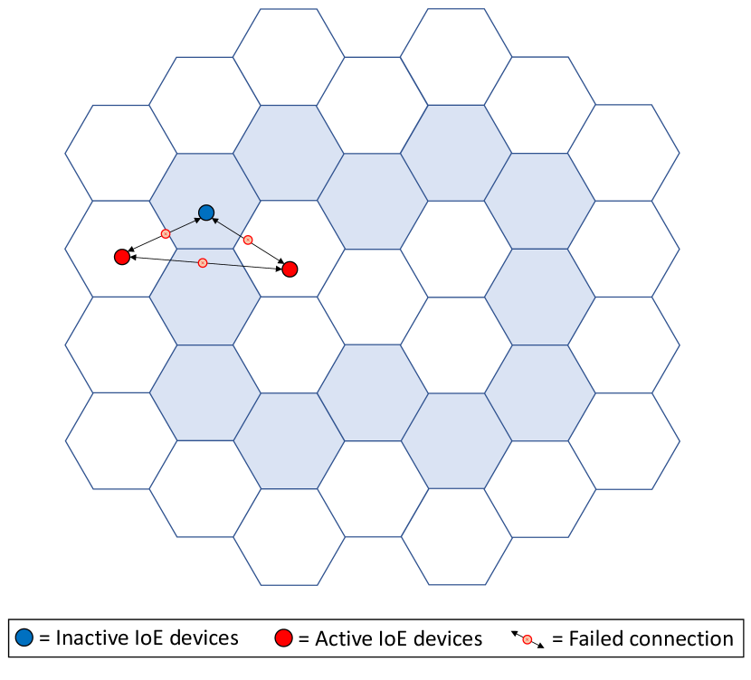
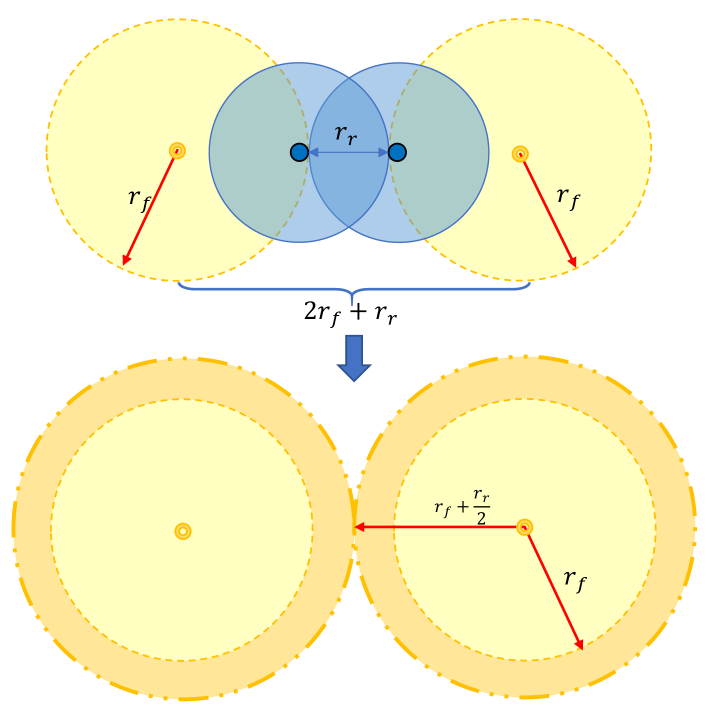
When the density of IoE devices is very large, we can safely assume that IoE devices within similar WET zones are forming connected components. However, for connected components of different WET zones to establish a connection and achieve non-zero percolation, we need to ensure the percolation of the Gilbert disk model shown in Fig.4 (referred to as “simple Gilbert disk model” in Lemma 23.
Lemma 5 (Approximation of critical ES density using a simple Gilbert disk model).
Using a simple Gilbert disk model , the approximation of critical ES density is written as:
| (23) |
Proof:
As shown in Fig.4, when is fixed, the distance between two ESs is . For non-zero percolation in Gilbert disk model , should satisfy
| (24) |
∎
Remark 4.
This model considers any ES and its nearby IoE devices as a whole. So this approximation is more suitable when is large enough. When is small, the value of this approximation is much less than the exact critical ES density, which is also not valid enough.
Though can approximate the critical ES density when is large, it can not replace when is small. Comparing the lower bound and upper bound, we propose a novel idea to combine the advantages of and without losing tractability.
IV-C Approximation from imitating bounds
The approximations and are suitable in different ranges of . In this part, we try to combine their advantages together. Similar to the lower bound and the upper bound, we use an expression like them to approximate the critical ES density in Lemma 26.
Lemma 6.
The approximation of critical ES density is written as:
| (25) |
where
| (26) |
Proof:
See Appendix C. ∎
This approximation is a combination of the approximations and . It is obtained by imitating the expressions of upper and lower bounds, which are compared in Table.II. We justify this approximate expression and propose a conjecture about the value of in Appendix C, which is in agreement with the upper bound of critical density for 2D site percolation in [48] and tight lower bound on the critical density for 2D Poisson RGGs in [49].
| Regime | Bound | Threshold |
| Sub-critical | Lower bound | |
| Super-critical | Upper bound | |
| Regime | Area of Envelope | Limit Value of Bound |
| Sub-critical | ||
| Super-critical | , where and |
V Simulation results and discussion
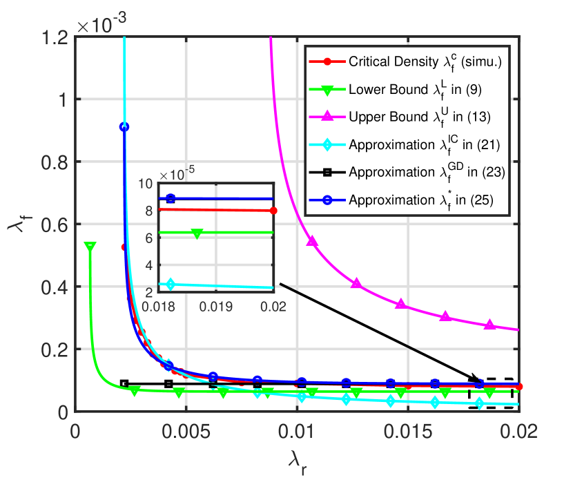
In this section we show simulation results for the percolation probability of the considered EaaS system compared to the derived bounds. We consider a 4000 m × 4000 m rectangular area and conduct Monte-Carlo simulations with 10,000 iterations. For each iteration, we consider that percolation occurs if we either have a giant connected component horizontally or vertically, where the distance between farthest two points is much larger than the D2D communication range and close to the simulation boundaries. We compute the average of critical ES density over all iterations. We put the bounds and approximations together in Fig.5. Based on [50, 51, 52, 53], it is common to assume that the maximum D2D communication distance is smaller than 40 m. The maximum WET range can be much larger than [54]. In the proposed system, the WET range of each ES is considered larger than the D2D communication range to ensure a sufficiently large energy supply range. Therefore, we set and . The simulation result is a curve between the lower bound and the upper bound . The value of the upper bound is always the highest, on the contrary, the value of the lower bound is always the lowest. and are suitable approximations in different range of . At the same time, is an approximation for all . When is small, the approximations and are similar, which are located between the upper and lower bound. The value of is much less than the simulation. When is large enough, the simulation , approximations and are matching, while is too small.
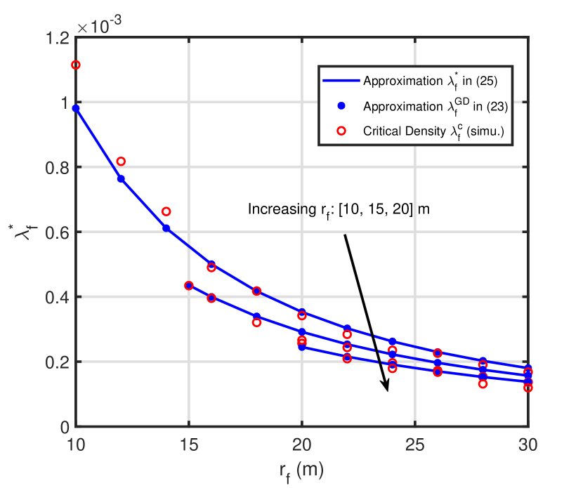
We also compare the approximation and simulation result in Fig.6 when which are matching with a small gap. When we choose different values of , the critical density decreases when increases.
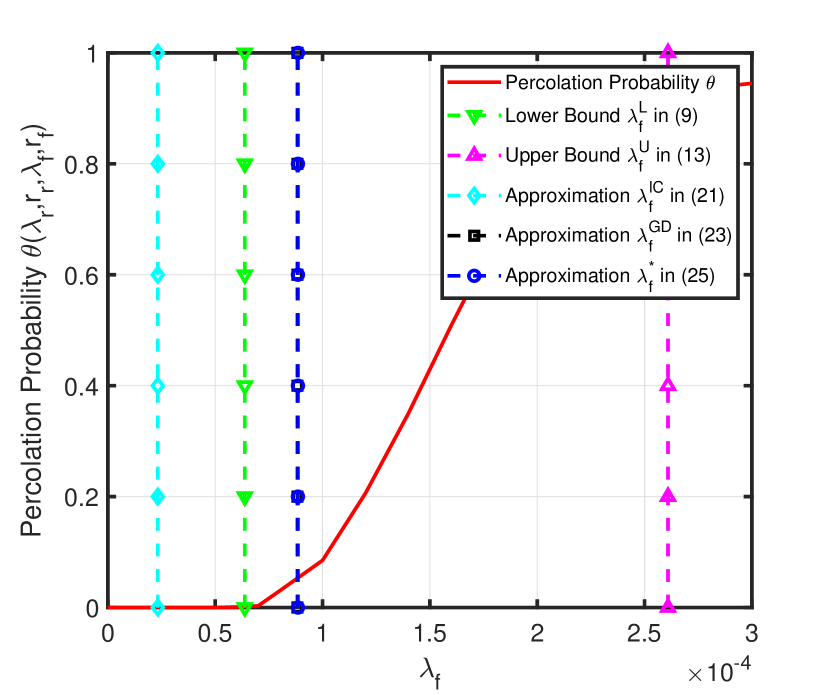
In Fig.7, we plot the curve of the simulation result of percolation probability in . We set , , and . The percolation probability is a non-decreasing function of . When is less than the lower bound , the percolation probability is 0. On the contrary, when is larger than the upper bound , the percolation probability is non-zero. The approximations and of the critical ES density are located between the lower bound and the upper bound .
To show the CAPEX gains, we can contrast the proposed percolation theory driven deployment against a full-coverage driven deployment. Recall that the critical ES density obtained by our percolation driven model aims to minimize the required density of ESs for full network connectivity. Alternatively, if the density of IoE devices is and ESs are deployed following a square lattice, the density of ESs for full-coverage is , which is times larger than the critical density obtained by our approximation . Therefore, in the considered rectangular area of dimensions, our percolation driven model can help reduce the cost of deploying more than 2700 ESs. However, the CAPEX saving of our percolation driven model comes at the cost of spatial power outages, which restricts the deployment of the IoE devices to utilize the offered EaaS. In particular, our percolation theoretic deployment reveals the minimum density of ESs that maintains large-scale connectivity of RF-power activated IoE devices but does not maintain 100% coverage of the spatial area. Based on the spatial randomness of the Gilbert disk model, the probability that an arbitrary location is not covered by the ESs is , which translates to approximately 0.5 for and . More comprehensive spatial coverage for the IoE devices would either require a higher density of ESs or a special arrangement (e.g., via batteries) for devices not covered by ESs.
It is worth noting that the theoretical analysis and simulations provided in this paper are based on an idealized system model. In realistic applications, the WET zones of ESs and D2D communication range can be limited by many factors, such as weather, terrain, buildings, vehicles, large metal machines, etc. Therefore, the WET zones of ESs are not always as regular as circular areas, and the critical ES density we obtain (i.e. the approximations ) becomes a lower bound of the actual ES density requirement. For realistic deployments, the lower bound serves as a guideline to estimate the actual ES density requirement to realize the large-scale connectivity first and reduce the potential CAPEX (i.e. redundant equipment manufacturing costs).
It is also worth noting that the considered ESs themselves are assumed to have perpetual energy sources by being connected to the electricity grid. However, for rural and remote areas, connecting every ES to the electricity grid may be infeasible. Therefore, the ESs may depend on random energy sources through solar panels or wind turbines. At the same time, the distribution of IoE devices can be scattered. Therefore, the large-scale multi-hop connectivity in rural and remote areas still needs to be further discussed.
The comparative analysis in the context of this paper shall mainly focus on comparing the WET EaaS platform for IoE against the classical battery-powered IoE. The performance of the battery-powered IoE can be considered as an upper bound for the WET EaaS-powered IoE, in which all IoE devices are activated by the electricity grid. However, it is significantly important to highlight the fact that battery-powered IoE can be placed in hard-to-reach or remote locations, making battery replacement/recharging a complicated process. In addition, the disposal of such batteries adds another level of complexity, especially when it needs to be done in an environment-friendly manner. All these aspects reflect the unique advantages of RF-powered IoE devices, which need to be included when comparing EaaS for IoE with battery-powered IoE. However, unlike connectivity and performance, which can be quantified through percolation theory as shown in this paper, the other aspects concerning the battery replacement/recharging difficulties and their disposal complexities are harder to quantify without more concrete operational data. In addition, to better investigate realistic IoE networks, it is expected to expand this EaaS platform to the case with heterogeneous IoE networks and heterogeneous ES networks.
VI Conclusions
This paper characterizes large-scale D2D connectivity of RF-powered IoE devices operating under EaaS platform, where energy providers deploy ESs that offer WET to power battery-less IoE devices. In this context, we develop a novel WET-aware connectivity random geometric graph assuming that the ESs and the D2D devices follow independent PPPs. Using percolation theory, we prove the existence of a finite critical ES density above which the WC-RGG operates in the super-critical regime, which implies network-wide large-scale D2D connectivity for the RF-powered IoE network. We show that the critical ES density decreases when the density of IoE devices increases. We also obtain approximations for the critical ES density by extending the classical percolation models, which can be used to estimate the ESs deployment CAPEX for successful EaaS service. In the derivation of approximations, we obtain an analytical value of critical density for continuum percolation in networks based on the 2D Gilbert disk model, where the maximum communication range between devices is 1 m, which is in agreement with existing work on percolation theory.
Appendix A Proof of Lemma 11
When we analyze the sub-critical regime, we assume that and . We consider two special cases: i) there is no IoE device in or ii) there is at least one IoE device and no ESs inside the outer envelope . The sufficient condition for no percolation can be expressed as:
| (27) |
The density of ESs should satisfy:
| (28) |
where
| (29) |
Then, the lower bound of critical ES density can be written as:
| (30) |
where
| (31) |
As shown in Fig.2(b), the area of the outer envelope can be calculated as:
| (32) |
In the sub-critical regime, we underestimate the probability of an inactive face and underestimate the value of the lower bound. But is still enough for the proof of phase transition. It is worth noting that the lower bound has a minimum value. When approaches , the value of approaches , and approaches .
Appendix B Proof of Lemma 2
When we analyze the super-critical regime, we assume that and . We consider a special case: there is at least one IoE device in and at least one ES inside the inner envelope . The sufficient condition for non-zero percolation is expressed as:
| (33) |
The density of ESs should satisfy:
| (34) |
where
| (35) |
Then the upper bound of critical ES density can be written as:
| (36) |
where
| (37) |
As shown in Fig.2, the side length of the hexagon is . The inner envelope is composed of six identical arcs with radius . Using the law of cosines,
| (38) |
We get
| (39) |
Using the law of sines,
| (40) |
Next, we have
| (41) |
The area of the inner envelope is
| (42) |
In the super-critical regime, we still underestimate the probability of an active face but overestimate the value of the upper bound. Similar to the lower bound, the upper bound can be also expressed as a non-increasing function of , which has a minimum value. When approaches , the value of approaches , and approaches .
Appendix C Proof of Lemma 26
In this part, we approximate the critical ES density by imitating the bounds. We compare the sub-critical regime and the super-critical regime in Table.II. These two bounds are both expressed as: . The main factors are the value of and the expression of . When is small, the values of bounds are decreasing sharply as increases. When approaches , the values of bounds are both expressed as . The trend of critical ES density function is similar to the bounds and the approximations we have obtained, so we propose to assume that the expression of critical density can be written using a similar way.
In Lemma 11 and 2, we know the limit values of the upper bound and lower bound are expressed using the areas of the outer envelope and inner envelope , respectively. Both these two areas are only relevant to and . We define the approximation is . Considering approximation , should satisfy:
| (43) |
Next,
| (44) |
When approaches , the value of approaches . To find the suitable value of , we adopt the necessary condition for percolation: . Let
| (45) |
Next, we have
| (46) |
where . Considering the sub-critical regime and super-critical regime, and . In some simulation-based approximations in literature [55], . But in this part, we obtain the theoretical value of for percolation in the infinite wireless network without simulation but just using theoretical analysis.
The expressions of areas of and are shown in (11) and (15), which are also compared in Table.II. When , and . When we set , the areas can be expressed as a function of and . They can be both considered as the product of and a function of .
For the sub-critical regime:
| (47) |
For the super-critical regime:
| (48) |
where and .
We define:
| (49) |
and
| (50) |
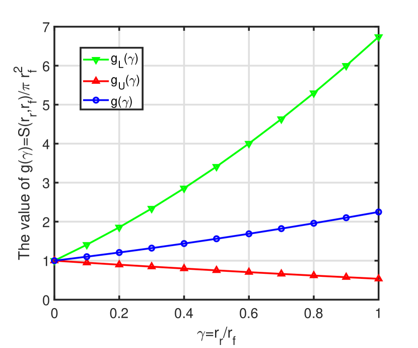
As shown in Fig.8, and both approach 1 when . We assume that
| (51) |
Due to , and . Because ,
| (52) |
Then, we have
| (53) |
To prove the feasibility of , we compare with :
| (54) |
In (54),
| (55) |
Then,
| (56) |
which means when is much larger than , the and are totally matching.
References
- [1] D. C. Nguyen, M. Ding, P. N. Pathirana, A. Seneviratne, J. Li, D. Niyato, O. Dobre, and H. V. Poor, “6G Internet of Things: A comprehensive survey,” IEEE Internet of Things Journal, vol. 9, no. 1, pp. 359–383, 2022.
- [2] B. Mao, F. Tang, Y. Kawamoto, and N. Kato, “AI models for green communications towards 6G,” IEEE Communications Surveys & Tutorials, vol. 24, no. 1, pp. 210–247, 2022.
- [3] X. Liu, N. Ansari, Q. Sha, and Y. Jia, “Efficient green energy far-field wireless charging for internet of things,” IEEE Internet of Things Journal, vol. 9, no. 22, pp. 23 047–23 057, 2022.
- [4] O. L. A. López, H. Alves, R. D. Souza, S. Montejo-Sánchez, E. M. G. Fernández, and M. Latva-Aho, “Massive wireless energy transfer: Enabling sustainable IoT toward 6G era,” IEEE Internet of Things Journal, vol. 8, no. 11, pp. 8816–8835, 2021.
- [5] S. Bi, Y. Zeng, and R. Zhang, “Wireless powered communication networks: An overview,” IEEE Wireless Communications, vol. 23, no. 2, pp. 10–18, 2016.
- [6] X. Lu, P. Wang, D. Niyato, D. I. Kim, and Z. Han, “Wireless networks with RF energy harvesting: A contemporary survey,” IEEE Communications Surveys & Tutorials, vol. 17, no. 2, pp. 757–789, 2015.
- [7] K. Huang and X. Zhou, “Cutting the last wires for mobile communications by microwave power transfer,” IEEE Communications Magazine, vol. 53, no. 6, pp. 86–93, 2015.
- [8] U. Paukstadt and J. Becker, “From energy as a commodity to energy as a service—a morphological analysis of smart energy services,” Schmalenbach Journal of Business Research, vol. 73, pp. 207–242, 2021.
- [9] P. Shepard, “EEPower,” 2019, accessed on Feb 3, 2023. [Online]. Available: https://eepower.com/news/clear-blue-technologies-launches-energy-as-a-service-for-wireless-power/
- [10] X. Ma, X. Liu, and N. Ansari, “Green laser-powered UAV far-field wireless charging and data backhauling for a large-scale sensor network,” IEEE Internet of Things Journal, vol. 11, no. 19, pp. 31 932–31 946, 2024.
- [11] D. B. West, Introduction to graph theory. Prentice hall Upper Saddle River, 2001, vol. 2.
- [12] R. Diestel, Graph Theory. Springer Berlin Heidelberg, 2017.
- [13] M. Haenggi, Stochastic geometry for wireless networks. Cambridge University Press, 2012.
- [14] M. Haenggi, J. G. Andrews, F. Baccelli, O. Dousse, and M. Franceschetti, “Stochastic geometry and random graphs for the analysis and design of wireless networks,” IEEE Journal on Selected Areas in Communications, vol. 27, no. 7, pp. 1029–1046, 2009.
- [15] H. ElSawy, A. Zhaikhan, M. A. Kishk, and M.-S. Alouini, “A tutorial-cum-survey on percolation theory with applications in large-scale wireless networks,” IEEE Communications Surveys & Tutorials, 2023.
- [16] O. Dousse, F. Baccelli, and P. Thiran, “Impact of interferences on connectivity in ad hoc networks,” IEEE/ACM Transactions on Networking, vol. 13, pp. 425 – 436, Apr. 2005.
- [17] M. Franceschetti, O. Dousse, D. N. C. Tse, and P. Thiran, “Closing the gap in the capacity of wireless networks via percolation theory,” IEEE Transactions on Information Theory, vol. 53, no. 3, pp. 1009–1018, March 2007.
- [18] P. C. Pinto and M. Z. Win, “Percolation and connectivity in the intrinsically secure communications graph,” IEEE Transactions on Information Theory, vol. 58, no. 3, pp. 1716 – 1730, Mar. 2012.
- [19] S. Goel, V. Aggarwal, A. Yener, and A. R. Calderbank, “The effect of eavesdroppers on network connectivity: A secrecy graph approach,” IEEE Transactions on Information Forensics and Security, vol. 6, p. 712–724, 2011.
- [20] W. Ren, Q. Zhao, and A. Swami, “Connectivity of heterogeneous wireless networks,” IEEE Transactions on Information Theory, vol. 57, no. 7, pp. 4315–4332, July 2011.
- [21] W. Ren, Q. Zhao, and A. Swami, “Temporal traffic dynamics improve the connectivity of ad hoc cognitive radio networks,” IEEE/ACM Transactions on Networking, vol. 22, no. 1, pp. 124–136, Feb. 2014.
- [22] Y. Liu, Y. Cui, and X. Wang, “Connectivity and transmission delay in large-scale cognitive radio ad hoc networks with unreliable secondary links,” IEEE Transactions on Wireless Communications, vol. 14, no. 12, pp. 7016–7029, Dec. 2015.
- [23] M. Yemini, A. Somekh-Baruch, R. Cohen, and A. Leshem, “The simultaneous connectivity of cognitive networks,” IEEE Transactions on Information Theory, vol. 65, no. 11, pp. 6911–6930, 2019.
- [24] J. Wang and X. Zhang, “Cooperative MIMO-OFDM-based exposure-path prevention over 3D clustered wireless camera sensor networks,” IEEE Transactions on Wireless Communications, vol. 19, no. 1, pp. 4–18, 2020.
- [25] L. Liu, X. Zhang, and H. Ma, “Optimal density estimation for exposure-path prevention in wireless sensor networks using percolation theory,” in Proc. of IEEE INFOCOM, 2012, pp. 2601–2605.
- [26] A. Zhaikhan, M. A. Kishk, H. ElSawy, and M.-S. Alouini, “Safeguarding the IoT from malware epidemics: A percolation theory approach,” IEEE Internet of Things Journal, vol. 8, no. 7, pp. 6039–6052, 2021.
- [27] Q. Wu, X. He, and X. Huang, “Connectivity of intelligent reflecting surface assisted network via percolation theory,” IEEE Transactions on Cognitive Communications and Networking, 2023.
- [28] Z. Han, G. Zhao, Y. Hu, C. Xu, K. Cheng, and S. Yu, “Dynamic bond percolation-based reliable topology evolution model for dynamic networks,” IEEE Transactions on Network and Service Management, 2024.
- [29] S. Ulukus, A. Yener, E. Erkip, O. Simeone, M. Zorzi, P. Grover, and K. Huang, “Energy harvesting wireless communications: A review of recent advances,” IEEE Journal on Selected Areas in Communications, vol. 33, no. 3, pp. 360–381, 2015.
- [30] H. S. Dhillon, Y. Li, P. Nuggehalli, Z. Pi, and J. G. Andrews, “Fundamentals of heterogeneous cellular networks with energy harvesting,” IEEE Transactions on Wireless Communications, vol. 13, no. 5, pp. 2782–2797, 2014.
- [31] T. T. Lam and M. Di Renzo, “On the energy efficiency of heterogeneous cellular networks with renewable energy sources—a stochastic geometry framework,” IEEE Transactions on Wireless Communications, vol. 19, no. 10, pp. 6752–6770, 2020.
- [32] A. S. Parihar, P. Swami, and V. Bhatia, “On performance of SWIPT enabled PPP distributed cooperative NOMA networks using stochastic geometry,” IEEE Transactions on Vehicular Technology, vol. 71, no. 5, pp. 5639–5644, 2022.
- [33] S. Kusaladharma, W.-P. Zhu, W. Ajib, and G. A. A. Baduge, “Stochastic geometry based performance characterization of SWIPT in cell-free massive MIMO,” IEEE Transactions on Vehicular Technology, vol. 69, no. 11, pp. 13 357–13 370, 2020.
- [34] A. H. Sakr and E. Hossain, “Analysis of -tier uplink cellular networks with ambient RF energy harvesting,” IEEE Journal on Selected Areas in Communications, vol. 33, no. 10, pp. 2226–2238, 2015.
- [35] M. Gharbieh, H. ElSawy, M. Emara, H.-C. Yang, and M.-S. Alouini, “Grant-free opportunistic uplink transmission in wireless-powered IoT: A spatio-temporal model,” IEEE Transactions on Communications, vol. 69, no. 2, pp. 991–1006, 2021.
- [36] F. Benkhelifa, H. ElSawy, J. A. Mccann, and M.-S. Alouini, “Recycling cellular energy for self-sustainable IoT networks: A spatiotemporal study,” IEEE Transactions on Wireless Communications, vol. 19, no. 4, pp. 2699–2712, 2020.
- [37] S. Kusaladharma, C. Tellambura, and Z. Zhang, “Evaluation of RF energy harvesting by mobile D2D nodes within a stochastic field of base stations,” IEEE Transactions on Green Communications and Networking, vol. 4, no. 4, pp. 1120–1129, 2020.
- [38] M. Chu, A. Liu, J. Chen, V. K. N. Lau, and S. Cui, “A stochastic geometry analysis for energy-harvesting-based device-to-device communication,” IEEE Internet of Things Journal, vol. 9, no. 2, pp. 1591–1607, 2022.
- [39] S. Enayati, H. Saeedi, H. Pishro-Nik, and H. Yanikomeroglu, “Optimal altitude selection of aerial base stations to maximize coverage and energy harvesting probabilities: A stochastic geometry analysis,” IEEE Transactions on Vehicular Technology, vol. 69, no. 1, pp. 1096–1100, 2020.
- [40] L. Ge, G. Chen, Y. Zhang, J. Tang, J. Wang, and J. A. Chambers, “Performance analysis for multihop cognitive radio networks with energy harvesting by using stochastic geometry,” IEEE Internet of Things Journal, vol. 7, no. 2, pp. 1154–1163, 2020.
- [41] Y. Meng, Z. Zhang, and Y. Huang, “Cache- and energy harvesting-enabled D2D cellular network: Modeling, analysis and optimization,” IEEE Transactions on Green Communications and Networking, vol. 5, no. 2, pp. 703–713, 2021.
- [42] M.-A. Lahmeri, M. A. Kishk, and M.-S. Alouini, “Stochastic geometry-based analysis of airborne base stations with laser-powered UAVs,” IEEE Communications Letters, vol. 24, no. 1, pp. 173–177, 2020.
- [43] K. Zhu, L. Xu, and D. Niyato, “Distributed resource allocation in RF-powered cognitive ambient backscatter networks,” IEEE Transactions on Green Communications and Networking, vol. 5, no. 4, pp. 1657–1668, 2021.
- [44] H. Sun, Z. Zhao, H. Cheng, J. Lyu, X. Wang, Y. Zhang, and T. Q. S. Quek, “IRS-assisted RF-powered IoT networks: System modeling and performance analysis,” IEEE Transactions on Communications, vol. 71, no. 4, pp. 2425–2440, 2023.
- [45] R. Meester and R. Roy, Continuum percolation. Cambridge University Press, 1996, vol. 119.
- [46] P. C. Pinto and M. Z. Win, “Percolation and connectivity in the intrinsically secure communications graph,” IEEE Transactions on Information Theory, vol. 58, no. 3, pp. 1716–1730, 2012.
- [47] Z. Yazdanshenasan, H. S. Dhillon, M. Afshang, and P. H. J. Chong, “Poisson hole process: Theory and applications to wireless networks,” IEEE Transactions on Wireless Communications, vol. 15, no. 11, pp. 7531–7546, 2016.
- [48] J. Kirkwood and C. E. Wayne, “Percolation in continuous systems,” 1983.
- [49] Z. Kong and E. M. Yeh, “Characterization of the critical density for percolation in random geometric graphs,” in 2007 IEEE International Symposium on Information Theory, 2007, pp. 151–155.
- [50] R. Z. Ahamad, A. R. Javed, S. Mehmood, M. Z. Khan, A. Noorwali, and M. Rizwan, “Interference mitigation in D2D communication underlying cellular networks: Towards green energy,” CMC-COMPUTERS MATERIALS & CONTINUA, vol. 68, no. 1, pp. 45–58, 2021.
- [51] S. Wang, O.-S. Shin, and Y. Shin, “Social-aware routing for multi-hop D2D communication in relay cellular networks,” in Proc. IEEE International Conference on Ubiquitous and Future Networks, 2019, pp. 169–172.
- [52] M. M. Salim, H. A. Elsayed, M. S. Abdalzaher, and M. M. Fouda, “RF energy harvesting dependency for power optimized two-way relaying D2D communication,” in Proc. IEEE International Conference on Internet of Things and Intelligence Systems, 2022, pp. 297–303.
- [53] Y. Zhao, Y. Li, H. Mao, and N. Ge, “Social-community-aware long-range link establishment for multihop D2D communication networks,” IEEE Transactions on Vehicular Technology, vol. 65, no. 11, pp. 9372–9385, 2016.
- [54] X. Lu, P. Wang, D. Niyato, D. I. Kim, and Z. Han, “Wireless networks with RF energy harvesting: A contemporary survey,” IEEE Communications Surveys & Tutorials, vol. 17, no. 2, pp. 757–789, 2014.
- [55] J. Quintanilla, S. Torquato, and R. M. Ziff, “Efficient measurement of the percolation threshold for fully penetrable discs,” Journal of Physics A: Mathematical and General, vol. 33, no. 42, p. L399, 2000.