Optimizing Likelihoods via Mutual Information: Bridging
Simulation-Based Inference and Bayesian Optimal Experimental Design

Abstract

Simulation-based inference (SBI) is a method to perform inference on a variety of complex scientific models with challenging inference (inverse) problems. Bayesian Optimal Experimental Design (BOED) aims to efficiently use experimental resources to make better inferences. Various stochastic gradient-based BOED methods have been proposed as an alternative to Bayesian optimization and other experimental design heuristics to maximize information gain from an experiment. We demonstrate a link via mutual information bounds between SBI and stochastic gradient-based variational inference methods that permits BOED to be used in SBI applications as SBI-BOED. This link allows simultaneous optimization of experimental designs and optimization of amortized inference functions. We evaluate the pitfalls of naive design optimization using this method in a standard SBI task and demonstrate the utility of a well-chosen design distribution in BOED. We compare this approach on SBI-based models in real-world simulators in epidemiology and biology, showing notable improvements in inference.

1 Introduction

Many scientific models are defined by a simulator that defines an output $y$ determined by the inputs, or designs, $\xi$, to a system, and parameters that define how the scientific model transforms the inputs to outputs, $\theta$. Inferring a posterior distribution of model parameters given data $p(\theta|y)$ is of central importance in Bayesian statistics and can be seen as a form of solving an inverse problem for a given simulator (Lindley, 1972). In SBI, a simulator forms an implicit probability distribution of the likelihood $p(y|\theta)$ that is used with the prior of the model parameters $p(\theta)$ to infer the posterior distribution of the scientific model parameters given the observed data, $p(\theta|y_{o})$. SBI methods aim to infer either the intractable likelihood or posterior using neural density estimators of the likelihood or posterior, or, classifiers to estimate the likelihood-to-evidence ratio, $\frac{p(\theta|y,\xi)}{p(\theta)}=\frac{p(y|\theta,\xi)}{p(y|\xi)}=\frac{p(y,\theta|\xi)}{p(\theta)p(y|\xi)}$ and refer to Cranmer et al. (2020) for a review of SBI methods.

Further, experimental data may be costly to collect. In drug development, collecting data is an expensive process that is partially responsible for the great cost associated with bringing new drugs to patients (Paul et al., 2010). For example, thousands to millions of designs may be employed per round of experimentation in a high-throughput screening campaign. Triaging which data points to gather can help reduce the time to develop a new therapy for patients. It is therefore important to prioritize collection of observed data $y_{o}$, using optimal designs $y_{o}|\xi^{*}$, to arrive at an accurate, but not overconfident, inference of model parameters to make predictions of future responses, such as the likelihood of successful drug treatment.

Meanwhile, Bayesian optimal experimental design (BOED) has shown promise as a method for optimizing experiments, even when dealing with potentially high-dimensional design spaces. This is achieved by employing a likelihood model, where a simulator generates samples as an implicit likelihood in the case of SBI, along with priors for the parameters of interest (Lindley, 1956; Foster et al., 2019; Kleinegesse and Gutmann, 2019). BOED operates by assessing the information gain that a given experimental design provides regarding parameters of a scientific model of interest. The information gain can only be evaluated after an experiment but Lindley (1956) defined the Expected Information Gain (EIG), $I(\xi)$, as the difference of entropy, $H$, of the prior to posterior as

$$I(\xi)\triangleq\operatorname{{}\mathbb{E}}_{p(y|\xi)}\left[H[p(\theta)]-H[p(\theta|y,\xi)]\right].$$ (1)

The EIG can be used as an approximation for the information gained in an experiment with design $\xi$. The intuition behind this process is that we must ask ourselves, which experimental design and outcome would be most surprising given what we assume about the model when conducting the experiment? This would be the optimal experimental design and can be rewritten into the form of calculating the mutual information (MI), where $\text{MI}(\theta;y|\xi)=I(\xi)$, between the observed data and unknown parameters as the ratio of likelihood to marginal likelihood or posterior to prior

$$\begin{split}\text{MI}(\theta;y|\xi)&=\mathbb{E}_{p(\theta)p(y|\theta,\xi)}\left[\log\frac{p(y|\theta,\xi)}{p(y|\xi)}\right]\\ &=\mathbb{E}_{p(\theta)p(y|\theta,\xi)}\left[\log\frac{p(\theta|y,\xi)}{p(\theta)}\right].\end{split}$$ (2)

Previous BOED work focused on estimating the MI as an objective function within an outer optimizer, such as Bayesian optimization, which results in a nested optimization process (Rainforth et al., 2018; Kleinegesse and Gutmann, 2020; Foster et al., 2019). This nested optimization can be inefficient, which lead to methods to simultaneously optimize the design and MI in a single optimization process (Foster et al., 2020). However, this unified optimization depended on an explicit likelihood or an implicit likelihood with a differentiable simulator (Kleinegesse and Gutmann, 2021; Ivanova et al., 2021), which is not available for many simulators in SBI.

Beginning with the similarity between Equation˜2 and SBI objective functions, we demonstrate a connection between BOED and SBI that uses either a surrogate of the likelihood, posterior, or the likelihood-to-evidence ratio through MI. We theoretically show how each type of SBI method can be optimized by maximizing the lower bound of MI shown in (2). We then show, theoretically and experimentally, how likelihood-based methods can be trained by maximizing the InfoNCE lower bound of MI (van den Oord et al., 2019), introducing a modified InfoNCE MI lower bound known as $I_{\text{NCE-}\lambda}$. Thus, we demonstrate how to simultaneously optimize an inference object for SBI while optimizing experimental designs, showing improvements over previous state of the art methods and allowing SBI methods to benefit from BOED.

While BOED methods are concerned with maximizing information gain of an experiment, many BOED methods do not consider the calibration or intermediate results of their resulting inference objects. This is a critical theme in SBI raised in (Hermans et al., 2022) where a SBI method aims to avoid producing overconfident or conservative posterior inferences. This is important in BOED as some methods may choose to split design optimization and inference objects between a design policy and critic, respectively. We therefore examine metrics of calibration and accuracy during BOED evaluation in our proposed method and against benchmark methods. We also examine how changing the $\lambda$ parameter within $I_{\text{NCE-}\lambda}$ influences EIG, calibration, and accuracy of posterior predictive distribution predictions.

In bridging BOED and SBI, our key contributions are:

• Novel MI Bound for Improved Inference: We introduce and analyze $I_{\text{NCE-}\lambda}$, a new MI bound, providing theoretical insights and empirical results that highlight its impact on calibration and predictive accuracy.

• Practical Optimization for Implicit Likelihoods: We propose a robust method to simultaneously optimize experimental designs and MI for SBI models without requiring a differentiable simulator. To address the limitations of naive gradient-based design optimization, we leverage a design distribution, significantly improving performance in non-differentiable settings.

• State-of-the-Art Calibration and Accuracy: Our approach achieves superior results in calibration and predictive accuracy compared to benchmark BOED methods, demonstrating its practical utility and setting a new standard for methods in this domain.

2 Background

2.1 Simulation-Based Inference

In many scientific disciplines, it is desirable to infer a distribution of parameters $\theta$, of a potentially stochastic model, or simulator, given observations, $y_{o}$. The closed-box simulator may depend on random numbers $z$, such as in stochastic differential equations, and previous experimental designs $\xi$, such that the simulator takes the form $y=g(\theta,\xi,z)$, or, may simply be simulated by non-differentiable operations. When a likelihood is not available, Approximate Bayesian Computation (ABC) methods can be used, which aims to create a surrogate of the likelihood function (Sisson et al., 2018). Recent deep-learning based SBI methods have outperformed ABC in many inference tasks (Lueckmann et al., 2021). Using a simulator to simulate the joint data distribution $(\theta,y)\sim p(y|\theta)p(\theta)$, using samples drawn from a prior $\theta\sim p(\theta)$, enables us to approximate an amortized likelihood $p_{\phi}(y|\theta)$ or posterior $p_{\phi}(\theta|y)$ distribution, which may be referred to as a neural density estimator. This is achieved by training the neural density estimator, such as a normalizing flow parameterized by $\phi$, to fit the observed data $y_{o}$ by maximum likelihood for the surrogate likelihood or posterior density (Papamakarios et al., 2021). Another SBI approach involves obtaining the likelihood-to-evidence ratio $\exp f_{\phi}(\theta,y)\approx\frac{p(y|\theta)}{p(y)}$ by training a classifier to differentiate parameters used in simulating observed values $y$ from the joint distribution or the product of marginals, $p(\theta)p(y)$. Different SBI methods can be used in inference for downstream applications depending on the desiderata of the inference task and have shown varying efficacy in different tasks (Lueckmann et al., 2021). For example, one might use an amortized posterior approximation if there are many different data samples to evaluate, whereas an ensemble of ratios was shown by Hermans et al. (2022) to perform more robustly on Simulation-Based Calibration (SBC) tests (Talts et al., 2020) at the cost of increased computational complexity.

Neural Likelihood Estimation   We can use data from the joint distribution to train a conditional neural density-based likelihood function (NL). If we take a dataset of samples $\{y_{n},\theta_{n}\}_{1:N}$ obtained from a simulator as previously described, we can train a conditional density estimator $p_{\phi}(y|\theta)$ to model the likelihood by maximizing the total log likelihood of $\sum_{n}\log p_{\phi}(y_{n}|\theta_{n})$, which is approximately equivalent to minimizing

$$\mathcal{L}_{\text{NL}}(\phi)=\operatorname{{}\mathbb{E}}_{p(\bm{\theta})}(D_{\text{KL}}(p(y|\theta)\|p_{\phi}(y|\theta))+\text{const},$$ (3)

where the Kullback-Leibler divergence is minimized when $p_{\phi}(y|\theta)$ approaches $p(y|\theta)$.

2.2 Normalizing Flows

Critical to likelihood and posterior-based SBI methods are density estimators, of which normalizing flows are a principled choice (Papamakarios et al., 2021; Kobyzev et al., 2020). A density estimator, denoted as $f_{\phi}(y)$, yields a real-valued output for any given data point across all possible values of $\phi$ that is normalized by design, ensuring a valid probability distribution. Normalization is enforced by the use of homeomorphisms from a base distribution to a data distribution. Specifically, starting from a known and normalized base distribution, $p(u)$, such as a Gaussian distribution, to the data distribution, $p(y)$, by a composition of nonlinear, monotonic, and invertible functions, $f:\mathbb{R}^{D}\rightarrow\mathbb{R}^{D}$, where $f$ is composed of $N$ functions, $f=f_{N}\circ\dots\circ f_{1}$. We map from a base distribution to target distribution using the change-of-variables formula as $p(y)=p(u)\rvert\det J(f)(u)\rvert^{-1},$ where $J(f)(u)$ is the Jacobian matrix of $f$ evaluated at $u$. A flow can be trained by minimizing the negative log likelihood of data $\{y_{n}\}_{n=1}^{N}$, which is also minimizing the forward KL divergence $D_{\text{KL}}[p^{*}(y)||p_{\phi}(y)]$ between a target distribution $p^{*}(y)$ and the flow model $p_{\phi}(y)$.

Normalizing flows are also a type of pathwise gradient estimator (Mohamed et al., 2020). Samples generated from the flow are determined by the function transformation $y\sim p(y|\theta,\xi)\hskip 5.0pt\Longleftrightarrow\hskip 5.0pty=f^{-1}(u;\theta,\xi)$, where $u\sim p(u)$ and $p(u)$ is the base noise distribution used to train the normalizing flow and can be used in variational inference (Rezende and Mohamed, 2015). Durkan et al. (2019) proposed Neural Spline Flow (NSF) that can be adapted for conditional estimation by parameterizing its polynomial spline bijectors with neural networks dependent on the data, $y$, as well as any information one may wish to include, such as $\theta\sim p(\theta)$ in the SBI setting. Now, the normalizing flow is trained on data from the joint distribution $(y,\theta)$ and can return the conditional distribution $p_{\phi}(\theta|y)$ or $p_{\phi}(y|\theta)$.

2.3 Bayesian Optimal Experimental Design

InfoNCE Bound   Following from Equation 2, Ivanova et al. (2021) proposed a lower bound of the MI based on the InfoNCE bound using an implicit likelihood with a differentiable simulator. They trained a design policy network $\pi_{\psi}$ that proposed designs based on the history of design-observation pairs, $h_{t-1}=\{(\xi_{i},y_{i})\}_{i=1:t-1}$ and a critic network $U_{\phi}$ that encapsulates the true likelihood when it maximizes the lower bound of MI. We adjust the bound to reflect the myopic experimental design setting (ignoring the design policy) and reformulate the bound as

$$\mathcal{L}_{\text{NCE}}(\xi,\phi;L)\coloneqq\operatorname{{}\mathbb{E}}\left[\log\frac{\exp(U_{\phi}(y,\xi,\theta_{0}))}{\frac{1}{L+1}\sum_{i=0}^{L}\exp(U_{\phi}(y,\xi,\theta_{i}))}\right],$$ (4)

where the expectation is over ${p(\theta_{0})p(y|\theta_{0},\xi)p(\theta_{1:L})}$, $\xi$ is the proposed design, $\theta_{0}$ is the original parameter that generated data $y$, generated from the differentiable simulator $p(y|\theta_{0},\xi)$, $L$ is the number of contrastive samples, and $U$ is a “critic” function such that $U\!:\!(y,\xi)\!\times\!\Theta\!\rightarrow\!\mathbb{R}$. This bound has low variance but is upper-bounded by $\log(L+1)$, potentially leading to large bias with insufficient contrastive samples. Additionally, previous work required a differentiable simulator to take gradients with respect to the inputs of the simulator, which may not be available in SBI settings.

3 SBI-BOED

We begin by noting the similarity in the different types of SBI and forms of MI from Equation (2) used in BOED. Indeed, each form of SBI can be cast in the MI framework. We show the relation between MI and SBI using generative models, which also allows for gradient-based optimization of non-differentiable simulators inputs.

3.1 Bridging SBI and BOED

We take inspiration from previous SBI and BOED methods to allow optimization of designs with respect to closed-box simulators that are modeled using normalizing flows. We start by noting how the loss function of contrastive ratio estimation (CRE) lower bounds Equation˜4

$$\log\frac{\exp(g_{\phi}(\theta_{0},y))}{\frac{1}{L}\sum_{\ell=1}^{L}\exp(g_{\phi}(\theta_{\ell},y))} \leq\log\frac{\exp(g_{\phi}(\theta_{0},y))}{\frac{1}{1+L}\sum_{\ell=0}^{L}\exp(g_{\phi}(\theta_{\ell},y))}$$ (5)

$$\hskip-30.00005pt=\log\frac{p_{\phi}(y|\theta_{0},\xi)}{\frac{1}{1+L}\sum^{L}_{\ell=0}p_{\phi}(y|\theta_{l},\xi)},$$

where $L$ is the number of contrastive samples, which is $K$ in CRE, and $g_{\phi}$ is a discriminative classifier, which holds for a single batch of data and constant experimental design, i.e. when $\xi$ is constant. We use a neural density estimator to create a Likelihood-Free version of Equation˜4. We now have a MI lower bound

$$\mathcal{L}_{\text{NCE}}(\xi,\phi;L)\coloneqq\operatorname{{}\mathbb{E}}\Bigg{[}\log\frac{p_{\phi}(y|\theta_{0},\xi)}{\frac{1}{1+L}\sum^{L}_{\ell=0}p_{\phi}(y|\theta_{l},\xi)}\Bigg{]}$$ (6)

where the expectation is over $p(\theta_{0})p(y|\theta_{0},\xi)p(\theta_{1:L})$. We can now simultaneously optimize designs and parameters of a neural density estimator. If we are to use a normalizing flow instead of a classifier as $\exp g_{\phi}(y,\theta,\xi)=p_{\phi}(y|\theta,\xi)$, then the lower bound of the MI holds since normalizing flows are normalized probability distribution functions. The result is an amortized likelihood at a potentially optimal experimental design. We discuss more SBI methods and their connection to MI optimization and BOED in Appendix˜C.

Finally, using a generative model such as a normalizing flow or diffusion model (Song and Ermon, 2020; Ho et al., 2020) trained with a maximum likelihood lower bound (Song et al., 2022) allows for gradients to be taken with respect to input designs in any automatic differentiation framework (Bradbury et al., 2018) by using a pathwise gradient estimator. Given this connection, we state our main theorem.

Theorem 3.1.

Maximizing the lower bound of the Mutual Information (MI) between parameters $\theta$ and observations $y$ in a Simulation-Based Inference (SBI) setting is equivalent to minimizing the Kullback-Leibler (KL) divergence, $D_{\text{KL}}(p(y|\bm{\theta})||p_{\phi}(y|\bm{\theta}))$, between the likelihood $p(y|\bm{\theta})$ and its approximation $p_{\phi}(y|\bm{\theta})$, and the marginal likelihood $p(y)$ and its approximation $p_{\phi}(y)$ given as

$$\begin{split}\max_{\phi}I_{\phi}(\theta;y)\Leftrightarrow&\min_{\phi}\big{[}\operatorname{{}\mathbb{E}}_{p(\theta)}D_{KL}(p(y|\theta)||p_{\phi}(y|\theta))\\ &+\operatorname{{}\mathbb{E}}_{p(y)}D_{KL}(p(y)||p_{\phi}(y))\big{]},\end{split}$$ (7)

where $I(\theta;y)$ is the mutual information between $\theta$ and $y$, and $I_{\phi}(\theta;y)$ is its approximation under parameter $\phi$.

More details and full proof of this theorem are in Section˜A.1.

3.2 Optimizing SBI-BOED

Regularization   Stability of the density estimator is a challenge when optimizing the MI lower bound due to data distribution shift as a result of changing $p(y|\theta,\xi)$ when optimizing $\xi$. To address this, we added a regularization term, $\lambda$, to help stabilize the training of the density estimator during design optimization as

$$\begin{split}\mathcal{L}_{\text{NCE-}\lambda}(\xi,\phi;L)\coloneqq&\operatorname{{}\mathbb{E}}\Bigg{[}\log\frac{p_{\phi}(y|\theta_{0},\xi)}{\frac{1}{1+L}\sum^{L}_{\ell=0}p_{\phi}(y|\theta_{l},\xi)}\\ &+\lambda\cdot\log p_{\phi}(y|\theta_{0},\xi)\Bigg{]}.\end{split}$$ (8)

where the expectation is over $p(\theta_{0})p(y|\theta_{0},\xi)p(\theta_{1:L})$. This regularization parameter gives more importance to accuracy of likelihood predictions when training where we provide theoretical analysis in Section˜B.1.

Algorithm 1 SBI-BOED

0: Simulator $p(y|\theta,\xi)$, Estimator $p_{\phi}(y|\theta,\xi)$,Number of experimental designs $T$,Number of BOED training steps $N$

0: Optimal designs $\{\xi^{*}_{i}\mid i=1,\ldots,T\}$,Approximate likelihood $p_{\phi}(y|\theta,\xi_{T}^{*})$

1: Initialize $\hat{p}_{0,0}(\theta)\leftarrow p(\theta)$

2: for $t=1,\ldots,T$ do

3:  Sample $\theta_{0:L}\sim\hat{p}_{t-1,0}(\theta)$

4:  for $n=1,\ldots,N$ do

5:   Sample $\xi\sim\mathcal{N}_{\text{trunc}}(\mu_{\xi}\mid\sigma_{n}^{2})$

6:   Simulate $y\sim p(y|\theta,\xi)$

7:   Estimate $\nabla\mathcal{L}_{\text{NCE}-\lambda}(\xi,\phi;L)$ via Equation˜8

8:   Update $\mu_{\xi}$ and $\phi$ using $\nabla_{\xi}$ and $\nabla_{\phi}$

9:   Checkpoint $\xi^{*}=\xi$ if $EIG_{\xi}>EIG_{\xi^{*}}$

10:  end for

11:  Observe $y_{o}$ using $\xi^{*}$ in an experiment

12: end for

Regularized Mutual Information Estimator   We integrate the regularization term $\lambda$ into a mutual information estimator and propose the InfoNCE-$\lambda$ objective

$$I_{\text{NCE-}\lambda}(\phi,\lambda)\coloneqq\operatorname{{}\mathbb{E}}_{p(\theta,y|\xi)}\left[\log\frac{p_{\phi}(y|\theta,\xi)^{1+\lambda}}{\frac{1}{1+L}\sum^{L}_{\ell=0}p_{\phi}(y|\theta_{l},\xi)}\right].$$ (9)

This formulation scales the likelihood term $p_{\phi}(y|\theta)$ with the regularization parameter $\lambda$. We provide a more thorough theoretical analysis of the influence of $\lambda$ on design optimization and predictive accuracy in Section˜B.1. Finally, while the bound on $I_{\text{NCE}}$ is $\log(L+1)$, we show in Section˜B.2 that a tighter bound incorporating the entropy term exists: $I_{\text{NCE-}\lambda}\leq\log(L+1)-\lambda\operatorname{{}\mathbb{E}}_{p(\theta)}H(y|\theta,\xi)$.

Design Distributions   A drawback of gradient-based methods is when there are sparse rewards, such as when the signal to noise ratio is, or approaches, zero. This results in designs struggling to optimize by gradient descent because optimizers may not be able to handle starting, or residing, in areas with no information. We demonstrate this failing in an ablation study in Section 5.3 and take inspiration from Reinforcement Learning’s (RL) use of a replay buffer (Lin, 1992; Mnih et al., 2013) by imposing a parameterized distribution of designs and optimizing parameters of that distribution to return more information.

When using design distributions, we compute the EIG for each individual observation $y_{i}$ associated with design $\xi_{i}$ and corresponding to the nominal parameter set $\theta_{0}$. In our usage, $\text{EIG}_{i}$ refers to the theoretical information gain expected from a single sample realization under design $\xi_{i}$, based on the current parameterization of the likelihood. It quantifies the information gain computed from a possible outcome as

$$\text{EIG}_{i}(\psi,\phi,L,\lambda)=\operatorname{{}\mathbb{E}}\Bigg{[}\log\frac{p_{\phi}(y_{i}|\theta_{0},\xi_{i})^{1+\lambda}}{\frac{1}{1+L}\sum^{L}_{\ell=0}p_{\phi}(y_{i}|\theta_{l},\xi_{i})}\Bigg{]},$$ (10)

with expectation over $p_{\psi}(\xi)p(\theta_{0})p(y|\theta_{0},\xi)p(\theta_{1:L})$ and where the parameter of the design distribution $\psi$ is optimized rather than the designs themselves.

We used a truncated Normal distribution for the design parameters, defined as $p_{\psi}(\xi)=\mathcal{N}_{\text{trunc}}(\mu_{\xi}|\sigma_{n}^{2})$, where $\mathcal{N}_{\text{trunc}}$ denotes a Normal distribution truncated within the bounds $[\alpha,\beta]$, and $\alpha$ and $\beta$ are the lower and upper bounds, respectively, and $\sigma$ that uses a decays schedule depending on the training round, $n$. Whenever the rewards are sparse, if the design distribution is initialized with sufficient support then it will contain an EIG with significantly more reward that can be updated with gradient descent. In our implementation, we used the reparameterization trick and a standard deviation schedule for $\sigma$ that decreased according to an exponential schedule $\sigma_{n}=\sigma_{\text{end}}+(\sigma_{\text{start}}-\sigma_{\text{end}})\cdot e^{-\frac{n*\rho}{N}}$, where $\sigma_{n}$ is the new standard deviation for the Normal distribution that parameterizes $\xi$ in training round $n$, $\sigma_{start}$ and $\sigma_{end}$ are hyperparameters for the initial and final variances respectively, $N$ is the total number of rounds, and $\rho$ is a decay rate hyperparameter.

Design Checkpoints   Checkpoints are used in supervised learning to save parameters that achieved low validation error (Vaswani et al., 2017; Devlin et al., 2019). Fujimoto et al. (2023) proposed the use of checkpoints in RL applications to save a policy that obtains a high reward during training to help improve performance at test time. Even with a distribution of designs, we found designs falling into a local minima during optimization, such as in Section˜C.3. We used design checkpoints to mitigate the risk of gradient-based designs falling into local minima that do not contain sufficient support to encapsulate the global minimum loss.

Posterior Inference   The likelihood trained on the optimized design can return approximate posterior samples by sampling $\hat{p}(\theta|y,\xi)\propto p_{\phi}(y|\theta,\xi)p(\theta)$. Should the likelihood be trained on i.i.d. data, then the joint factorizes to product likelihood $p_{{\theta}}\left(y_{1,\dots,N}|\theta,\xi_{1,\dots,N}\right)=\prod_{i=0}^{N}p(y_{i}|\theta,\xi_{i})$ which can be used in Markov chain Monte Carlo (MCMC) to draw posterior samples.

4 Related Work

In BOED, we focus on the setting of myopic gradient-based experimental design. Previously, Foster et al. (2019) proposed various likelihood-free information bounds that could work in the SBI setting based on variational inference estimators but did not make use of a normalized generative model like a normalizing flow. This is problematic for use in sequential SBI methods that make use of a normalized likelihood or posterior functions. Kleinegesse and Gutmann (2020) developed MINEBED to simultaneously optimize experimental designs and a critic that could draw samples from the posterior, but relied on a differentiable simulator or using Bayesian Optimization. Ivanova et al. (2021) extended both previous works and developed policy-based experimental designs for non-myopic experimental designs, but whose critics also relied on differentiable simulators - simulators whose inputs can be connected to a differentiable computation graph, which may not be available for scientific simulators. A RL approach (Lim et al., 2022) optimized a critic without requiring a differentiable simulator but relies on computationally expensive RL algorithms and may not be feasible for practitioners with scientific simulators that can take significant amount of time to simulate. This is exemplified in our biological experiment where each round of simulation takes about ten seconds.

Recent work connecting SBI methods to MI-based optimization studied how to stably train a discriminative and generative SBI model (Miller et al., 2023), and applying a nonparametric function to the selection of data points to reduce variance of the resulting MI estimate (Glaser et al., 2022). These methods take a complimentary approach to ours but require a generative and discriminative model whereas we only require a generative model. Additionally, we study the utility of MI-based optimization of SBI models in BOED.

Figure 1: Comparison on the Two Moons task of the EIG and the validation loss $-\operatorname{{}\mathbb{E}}\log p_{\phi}(y|\theta)$ across varying number of contrastive samples ($L=N-1$) and $\lambda$ regularization. Increasing number of contrastive samples improves the information lower bound and likelihood validation metrics. The $\lambda$ parameter helps improve the likelihood accuracy at the expense of MI estimation.

5 Experiments

We evaluate SBI-BOED in one SBI task and three experimental design tasks, two where the designs are i.i.d. and another that is time-dependent. We first evaluate the MI lower bound estimation performance in high-dimensional design spaces in a simple linear model to understand the performance of SBI-BOED as it scales with the number of design dimensions and to evaluate the importance of regularization. We then evaluate SBI-BOED on sequential design tasks in both a time-dependent and i.i.d. setting, and benchmark against comparable methods. MINEBED-BO is a technique for estimating the MI using a neural network and then using Bayesian optimization to optimize designs (Kleinegesse and Gutmann, 2020). We compare against iDAD (Ivanova et al., 2021) and differentiable MINEBED (Kleinegesse and Gutmann, 2021) in the myopic design setting of a single experimental design to compare with SBI-BOED methods. In all experiments we compare all models to a measure of MI lower bound, the Expected Information Gain (EIG), a visual analysis of posterior samples drawn by the No-U-Turn Sampler method of MCMC sampling, and the L-C2ST metric of local evaluation of the posterior given an observed data point $y_{o}$ (Linhart et al., 2024). To the best of our knowledge, the L-C2ST metric is the only quantitative assessment of the calibration of an inference model. We also show SBC plots for our methods but the L-C2ST provides an easier comparison among models by indicating whether the observed data point is generated by the posterior of the model of interest. All experiment details, such as hyperparameters, can be found in Appendix˜D.

5.1 Evaluation of the MI on Two Moons

We first study how well our amortized generative model performs in the non-experimental design setting. This is to gain insight into the tradeoffs between regularization of the objective in Equation˜8 and choice of the number of contrastive parameters $L$ in the Equation˜4. As noted by Miller et al. (2024); Glaser et al. (2022) when optimizing the MI between $y$ and $\theta$ there is a decrease in the validation accuracy, $\operatorname{{}\mathbb{E}}\log p_{\phi}(y|\theta)$. We investigate the effect of $\lambda$ regularization in the objective Equation˜8 on the information gained, as measured by the EIG, and the validation log probability. The resulting sweep can be seen in Figure˜1. Increasing the number of contrastive parameters both helps to improve the information gained and the validation loss. We note that optimization using the Equation˜4 and the parameters we chose did not ameliorate the known issue of mode collapse of likelihood-based functions in the two moons task as shown by Greenberg et al. (2019). We show an example in Appendix˜E.

Figure 2: Comparison of the EIG across design dimensions, type of BOED, and $\lambda$ regularization for the noisy linear model examining the moving average over 10 different random seed initializations. For the single design dimension, all SBI-BOED regularizaiton levels generally similar, with the non-regularized version being the closest to the optimal MI bound. In the higher-dimension design cases, SBI-BOED increases its EIG with more designs. In the 100-dimensional design case, we see the benefit of using $\lambda$ regularization to stabilize the training of a design-dependent normalizing flow in high-dimensional input space at the cost of slightly lower EIG.

5.2 Noisy Linear Model

In our first BOED task, we evaluate how SBI-BOED performs on the EIG metric with increasing design dimensions. We follow Kleinegesse and Gutmann (2020) and evaluate optimal designs on a noisy linear model where a response variable $y$ has a linear relationship with experimental designs $\xi$, which is determined by values of the model parameters $\bm{\theta}=[\theta_{0},\theta_{1}]$, which model the offset and gradient. We would like to optimize the value of $D$ measurements to estimate the posterior of $\bm{\theta}$, and so create a design vector $\bm{\xi}=[\xi_{1},\dots,\xi_{D}]^{\mathsf{T}}$. Each design, $\xi_{i}$ returns a measurement $y_{i}$, which results in the data vector $\bm{y}=[y_{1},\dots,y_{D}]^{\mathsf{T}}$. We use a Gaussian noise source $\mathcal{N}(\epsilon;0,1)$ and Gamma noise source $\Gamma(\nu;2,2)$. The model is then

$$\bm{y}=\theta_{0}\bm{1}+\theta_{1}*\bm{\xi}+\bm{\epsilon}+\bm{\nu},$$ (11)

where $\bm{\epsilon}=[\epsilon_{1},\dots,\epsilon_{D}]^{\mathsf{T}}$ and $\bm{\nu}=[\nu_{1},\dots,\nu_{D}]^{\mathsf{T}}$ are i.i.d. samples. We used a prior distribution on model parameters as $p(\bm{\theta})=\mathcal{N}(\bm{\theta};0,3^{2})$. We evaluate SBI-BOED, purely using design gradients and no distribution over designs, to examine how changing the $\lambda$ regularization parameter in Equation˜8 influences the resulting MI bound and design optimization stability with increasing design dimension.

For all design dimensions, we randomly initialize designs $\xi\in[-10,10]$. For SBI-BOED, we chose $N=10$, the number of batch samples $\bm{y}\sim p(\bm{y}|\theta_{0},\bm{\xi})$, and $L=50$ contrastive samples. We used a neural spline flow with training details in Appendix˜D. We show the plots of the EIG in Figure˜2, where we can see that SBI-BOED optimizes a lower bound of MI, which increases for higher design dimensions. This corresponds with intuition that gathering more data results in more information. Similar to the two moons task, we see how the choice of $\lambda$ influences the stability of MI estimation for SBI-BOED in high design dimensions where there seems to be a tradeoff with choice of regularization and MI estimation. This may be due to regularization limiting gradient updates of designs that lead to out of distribution data distributions, but is balanced by the stability in the training objective.

5.3 SIR Model

We next evaluate the performance of SBI-BOED with different amounts of regularization on a real-world implicit likelihood model that has a differentiable simulator as a comparison to alternative methods. We use the Susceptible, Infected, or Recovered (SIR) epidemiology model specified in Ivanova et al. (2021). The SIR model represents a fixed population that has three groups: susceptible, infected, and recovered. Individuals transition from susceptible to infected with a parameter $\beta$ and from infected to recovered with parameter $\gamma$. Therefore, the model parameters are $\theta\coloneqq[\beta,\gamma]$ and the design space $\Xi$, consists of a time $\kappa$ to measure individuals to infer parameters $\theta$. We measured the EIG, L-C2ST, and median distance from the observed data point to samples generated by the final posterior distribution.

Table 1: SIR (Section 5.3) and BMP (Section 5.4) results: comparison of EIG, L-C2ST, and median distance (Med.) on five BOED methods for two tasks with T=2 experimental design rounds for the SIR model and T=3 for the BMP model. We used the same number of contrastive samples for iDAD and MINEBED as with SBI-BOED and report mean and standard error of results over 3 experiments using different seeds.

Method	SIR (T=2)			BMP (T=3)
	EIG $(\uparrow)$	L-C2ST $(\downarrow)$	Med. $(\downarrow)$	EIG $(\uparrow)$	L-C2ST $(\downarrow)$	Med. $(\downarrow)$
MINEBED(-BO)	2.69 $\pm$ 0.03	0.07 $\pm$ 0.05	71.26 $\pm$ 5.66	9.05 $\pm$ 0.20	0.23 $\pm$ 0.01	0.87 $\pm$ 0.08
iDAD (InfoNCE)	2.67 $\pm$ 0.02	0.10 $\pm$ 0.04	71.65 $\pm$ 2.78	N/A	N/A	N/A
SBI-BOED ($\lambda=1$)	1.01 $\pm$ 0.03	0.05 $\pm$ 0.01	47.99 $\pm$ 2.62	10.39 $\pm$ 0.01	0.002 $\pm$ 0.002	0.61 $\pm$ 0.01
SBI-BOED ($\lambda=0.1$)	1.47 $\pm$ 0.23	0.03 $\pm$ 0.01	46.85 $\pm$ 3.21	10.38 $\pm$ 0.01	0.001 $\pm$ 0.001	0.60 $\pm$ 0.01
SBI-BOED ($\lambda=0.01$)	1.63 $\pm$ 0.23	0.04 $\pm$ 0.02	52.85 $\pm$ 0.70	10.39 $\pm$ 0.01	0.004 $\pm$ 0.002	0.61 $\pm$ 0.01

Table˜1 summarizes the results. We find that iDAD and differentiable MINEBED achieve the best information gain, likely thanks to using differentiability of the simulator, but perform worse than SBI-BOED on L-C2ST and median distance metrics. This may indicate the learned critic is not as accurate as the amortized likelihood trained in SBI-BOED. Among SBI-BOED methods, we see that more regularization generally leads to improved median distance, and all perform rouglhy the same on calibration. Thus, improved information gain does not necessarily correlate with improved downstream prediction, as measured by the median distance metric. This highlights an important caveat to BOED methods that we should not rely on a single metric and holistically assess the resulting inference model in terms of accuracy and calibration before making decisions (performing experiments). We find that the posterior estimates are generally consistent with the ground truth. We show an example posterior form our method in Appendix˜F with ground truth parameters $\theta=[0.7399,0.0924]$.

Ablation Study   We compare the performance of SBI-BOED with and without a design distribution when maximizing the EIG in Figure˜3 in the first round of design optimization. The prior used in the SIR model creates a challenge for myopic and local design optimization by introducing regions with little EIG signal, such as the flatter part of the SIR curve shown in Appendix˜F. The design distribution overcomes this challenge by querying diverse sets of designs with better gradients to optimize Equation˜8.

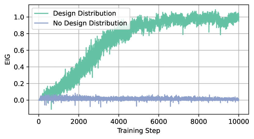
Figure 3: Training (higher is better) without a design distribution in the first round of optimization for the SIR model fails to find designs with high rewards.

5.4 Bone Morphogenetic Protein Model

The Bone Morphogenetic Protein (BMP) pathway is important in developmental and disease processes. A mass action kinetics model was proposed for the BMP pathway (Antebi et al., 2017). The one-step model proposed by Su et al. (2022) models type I (A) and type II (B) receptors coupling with a ligand (L) to form a trimer complex (T) with equilibrium affinity $K$ in a single step as $A+B+L\autorightleftharpoons{$K$}{}T$. The trimeric complex then phosphorylates SMAD protein to send a downstream gene expression signal, $S$, with a certain efficiency, $\varepsilon$ as $\varepsilon T=S$. Steady-state gene expression signals can be simulated using convex optimization in a closed-box optimization process. Thus, we would like to infer the parameters $K$ and $\varepsilon$ given data, $S$. In the experimental design context, we would like to optimize the ligand concentration, $\bm{L}^{*}$, used in an experiment so to gain the most information about the parameters of this model of a biological signaling pathway. The model parameters are $\theta\coloneqq[K,\varepsilon]$ and we use ground truth parameters $\theta=[0.85,0.85]$. We show an example of the prior predictive equation in Appendix˜F. We evaluated a 1D design dimension for the ligand concentration on a uniform range from $10^{-3}\text{ng/mL}$ to $10^{3}\text{ng/mL}$. We compare against the same benchmarks except the iDAD algorithm, which cannot work on this non-differentiable simulator. We train the EIG for 500 steps in each design optimization round because of the expensive simulation time required in each round (about 15 seconds).

All SBI-BOED design algorithms perform well in this setting, partially due to the bias in larger concentrations containing more information. However, we see that SBI-BOED methods outperform the competing method of MINEBED combined with Bayesian optimization in all metrics. Again, the model with the best EIG does not correspond to the most-calibrated model nor the best accuracy predictions. Given that our models start from an uninformative uniform prior, the posterior in the last round approaches the true value while leaving uncertainty to mitigate overconfidence Appendix˜F.

6 Discussion

We demonstrated the connection between optimizing a lower bound of mutual information typical in BOED settings and optimizing a likelihood from SBI settings. We evaluated the accuracy of the generative model’s likelihood approximation on a standard SBI benchmark to show the tradeoff of the number of contrastive samples to the regularization used. We also evaluated the effect of the regularization parameter on BOED tasks to comparable methods keeping contrastive samples constant. Besides regularization, we also presented novel methods to overcome pitfalls in optimizing designs for purely generative models, including using a distribution over designs and design checkpoints. We found that SBI-BOED performed better in predictive accuracy and calibration, and sometimes better in EIG, on a benchmark of comparable BOED methods on two scientific simulators, one that was and one that was not differentiable w.r.t. designs. Thus, we demonstrated the importance of more holistic examination of BOED methods given that a design with greater information gain may not lead to better downstream prediction accuracy. Indeed, metrics such as calibration play important roles in scientific decision-making, and our work highlights the importance of including such measures when designing experiments within BOED methods. This motivates future work to consider calibration and predictive accuracy while optimizing designs.

We used normalizing flows as surrogates for the likelihood but any generative model can be used as a surrogate given that its likelihood, or its bound, can be evaluated. This opens opportunities for BOED to any likelihood-based model used with, for example, diffusion (Ho et al., 2020; Song and Ermon, 2019) or flow-matching, (Lipman et al., 2023) each of which may handle higher-dimensional data better or provide novel opportunities to optimize experiments by increased flexibility of design optimization in the data or noise space (Ben-Hamu et al., 2024).

Appendix A Mutual Information-Based Likelihood Optimization Derivation & Proofs

We provide a derivation and proof of how optimizing a lower bound of the mutual information is the same as minimizing the KL divergence in (3). We also discuss alternative BOED bounds and how adding a distribution of designs to the MI approximation keeps it a valid lower bound.

A.1 Derivation of Optimization of the Mutual Information

We investigate how optimizing the mutual information within the SBI-BOED loss framework leads to an implicit optimization of the likelihood. Following the approach outlined by [Miller et al., 2024], we optimize our approximation to the true likelihood by minimizing the KL divergence:

$$D_{\text{KL}}(p(y|\theta)||p_{\phi}(y|\theta)).$$ (12)

Within the SBI framework, we draw samples of parameters $\theta$ from the prior $p(\theta)$ and of data $y$ conditioned on these parameters from the likelihood $p(y|\theta)$. This sampling enables us to approximate the expected KL divergence across the parameter space:

$$\mathbb{E}_{p(\theta)}[D_{\text{KL}}(p(y|\theta)||p_{\phi}(y|\theta))].$$ (13)

Now we express the KL divergence as the expectation of the log ratio of probabilities:

$$\mathbb{E}_{p(\theta)}[D_{\text{KL}}(p(y|\theta)||p_{\phi}(y|\theta))] =\mathbb{E}_{p(\theta,y)}\left[\log\frac{p(y|\theta)}{p_{\phi}(y|\theta)}\right]$$ (14)

$$=\mathbb{E}_{p(\theta,y)}\left[\log\frac{p(y|\theta)}{p(y)}\frac{p(y)}{p_{\phi}(y|\theta)}\right]$$ (15)

$$=I(\theta;y)+\mathbb{E}_{p(\theta,y)}\left[\log\frac{p(y)}{p_{\phi}(y|\theta)}\right]$$ (16)

$$=I(\theta;y)+\mathbb{E}_{p(y)}\left[\log p(y)\right]-\mathbb{E}_{p(\theta,y)}\left[\log p_{\phi}(y|\theta)\right].$$ (17)

Since the KL divergence is always non-negative, the optimization process aims to find the parameters $\phi$ that minimize this expected divergence (approaches 0), implicitly maximizing the mutual information between parameters.

We now base our proof of Theorem˜3.1 as follows:

Proof.

Let us consider the MI between random variables $\Theta$ and $Y$, where $y\sim Y$ and $\theta\sim\Theta$, then we have

$$I(\theta;y)=\mathbb{E}_{p(\theta,y)}\left[\log\frac{p(y|\theta)}{p(y)}\right].$$ (18)

In the SBI setting, we would like to approximate the likelihood $p_{\phi}(y|\theta)$. We can approximate the marginal likelihood by the Strong Law of Large Numbers using $\operatorname{{}\mathbb{E}}_{p(\theta)}\big{[}p(y|\theta)\big{]}=\int_{\theta}p(y|\theta)p(\theta)d\theta\approx\frac{1}{L}\sum_{\ell}^{L}p(y|\theta_{\ell})$. The bound gets tighter as $L\rightarrow\infty$ and as the likelihood better-approximates the true likelihood. Assuming we are optimizing the parameters $\phi$ to maximize this objective, then we have

$$\hat{\phi} =\underset{\phi}{\arg\max}\;\operatorname{{}\mathbb{E}}_{p(\theta,y)}\left[\log\frac{p_{\phi}(y|\theta)}{\hat{p}(y)}\right]$$ (19)

$$=\underset{\phi}{\arg\min}\;\left(I(\theta;y)-\operatorname{{}\mathbb{E}}_{p(\theta,y)}\left[\log\frac{p_{\phi}(y|\theta)}{\hat{p}(y)}\right]\right)$$ (20)

$$=\underset{\phi}{\arg\min}\;\operatorname{{}\mathbb{E}}_{p(\theta,y)}\left[\log\frac{p(y|\theta)}{p(y)}\frac{\hat{p}(y)}{p_{\phi}(y|\theta)}\right]$$ (21)

$$\approx\underset{\phi}{\arg\min}\;\left(\operatorname{{}\mathbb{E}}_{p(\theta)}D_{KL}(p(y|\theta)||p_{\phi}(y|\theta))-\operatorname{{}\mathbb{E}}_{\hat{p}(y)}D_{KL}(\hat{p}(y)||p(y))\right)$$ (22)

$$=\underset{\phi}{\arg\min}\left(\operatorname{{}\mathbb{E}}_{p(\theta)}D_{KL}(p(y|\theta)||p_{\phi}(y|\theta))+\operatorname{{}\mathbb{E}}_{\hat{p}(y)}\left[\log\hat{p}(y)\right]-\text{const.}\right)$$ (23)

where the marginal likelihood is approximated as $\hat{p}(y)=\frac{1}{L}\sum_{i=1}^{L}p_{\phi}(y|\theta_{i}),\quad\theta_{i}\sim p(\theta)$. Thus, maximizing the InfoNCE bound from Equation˜4, returns an optimized likelihood minimizing the same objective in Equation˜3 with an additional penalty on marginal likelihood approximation, which depends on the number of contrastive samples $L$.

∎

Remark. In the BOED setting, the MI is simply conditional on a design, $\xi$, as $I(\theta;y|\xi)$ which allows for gradient-based optimization by a pathwise gradient estimator as detailed in Section˜2.2. An interesting insight to this derivation is that InfoNCE bound used to maximize a lower bound of MI may be biased by the reverse KL of the marginal likelihood to models that better represent the data. This may surface in BOED with designs preferring models that do not cover enough of the potential parameter spaces that explain the data.

A.2 Ensuring a Valid MI Objective with Design Distributions

One of the main assumptions of this paper is that using a distribution over designs, $p(\xi)$, keeps a valid bound of the MI. The joint density of $y$ and $\xi$ has a density with respect to Lebesgue measure on $\Xi\times\mathcal{Y}$ since

$$p(y,\xi|\theta)=p(\xi)p(y|\theta,\xi),$$ (24)

where $p(\xi)$ represents the Normal distribution, $\mathcal{N}_{t}(\mu_{\xi}|\sigma^{2}_{n})$ that may depend on the result of the previous round to determine its starting position. Putting a distribution on designs can be seen as using a stochastic policy, similar to noise levels used in RL. Given the joint distribution of observations and designs, the conditional mutual information $I(\theta;y|\xi)$, which quantifies the information about parameters $\theta$ obtained through observations $y$, conditioned on designs $\xi$, remains valid under the distribution $p(\xi)$. Mathematically, this is represented as:

$$I(\theta;y|\xi)=H(y|\xi)-H(y|\theta,\xi)$$ (25)

provided $p(\xi)$ is a valid probability distribution, where each individual entropy term is given by

$$H(y|\xi)=-\int_{\mathcal{Y}}\int_{\Xi}p(y,\xi)\log p(y|\xi)d\xi dy,$$ (26)

and

$$H(y|\theta,\xi)=-\int_{\mathcal{Y}}\int_{\Theta}\int_{\Xi}p(y,\theta,\xi)\log p(y|\theta,\xi)d\xi d\theta dy.$$ (27)

This invariance is due to the fact that $\xi$ serves as a known conditional variable that structures the calculation of mutual information without contributing additional information about $\theta$ beyond the observed data $y$. Hence, adding a probability distribution on designs retains a valid measure of MI. While we used a simple tempered design distribution, they can be parameterized with more sophisticated models akin to policy networks in RL and used in BOED by [Foster et al., 2021, Ivanova et al., 2021]. We leave this for future work.

Appendix B Theoretical Analysis of SBI-BOED Components

We provide more theoretical analysis of the impact of the $\lambda$ parameter of $I_{\text{NCE-}\lambda}$ on predictive accuracy, estimating the EIG, and gradients of EIG and normalziing flow model parameters, $\phi$.

B.1 Theoretical analysis of the $\lambda$ regularization parameter

We experimentally demonstrated in Section˜5.1 that the $\lambda$ regularization parameter in SBI-BOED influences both the likelihood’s validation accuracy and the EIG bound. We theoretically analyze both scenarios as well as $\lambda$ influence on optimization gradients in the following sections.

Influence of $\lambda$ on likelihood prediction accuracy   Starting from Equation˜21 of the previous section, including the $\lambda$ regularization parameter results in

$$\hat{\phi} =\underset{\phi}{\arg\min}\;\operatorname{{}\mathbb{E}}_{p(\theta,y)}\left[\log\frac{p(y|\theta)}{p(y)}\frac{\hat{p}(y)}{p_{\phi}(y|\theta)}\right]+\lambda\operatorname{{}\mathbb{E}}_{p(\theta,y)}\log[p_{\phi}(y|\theta)]$$ (28)

$$=\underset{\phi}{\arg\min}\;\operatorname{{}\mathbb{E}}_{p(\theta,y)}\left[\log\frac{p(y|\theta)}{p(y)}\frac{\hat{p}(y)}{p_{\phi}(y|\theta)}p_{\phi}(y|\theta)^{\lambda}\right].$$ (29)

We now focus on the contribution of the added $p_{\phi}(y|\theta)^{\lambda}$ term grouped with the likelihood’s KL divergence from Equation˜23. Reformulating this term, we express the $\lambda$-regularized KL divergence as

$$D_{\text{KL}}(p(y|\theta)\|p_{\phi}(y|\theta)^{1-\lambda}) =\mathbb{E}_{p(y|\theta)}\left[\log\frac{p(y|\theta)}{p_{\phi}(y|\theta)^{1-\lambda}}\right]$$ (30)

$$=\mathbb{E}_{p(y|\theta)}\left[\log p(y|\theta)-(1-\lambda)\log p_{\phi}(y|\theta)\right].$$ (31)

This modified divergence adjusts the weighting of the log-likelihood term $\log p_{\phi}(y|\theta)$ based on $\lambda$. We show how $\lambda$ influences optimization, omitting the trivial case when $\lambda=0$:

• For $\lambda>0$: The term $(1-\lambda)$ reduces the weight of the approximate likelihood, ensuring broad coverage of the parameter space while emphasizing accuracy.

• For $\lambda<0$: The term $(1-\lambda)>1$ amplifies the weight of the approximate likelihood, leading to mode-seeking behavior that prioritizes high-probability regions at the expense of the tails.

Influence of $\lambda$ on the EIG   We start from Equation˜9 and rephrase it here using the shortened marginal likelihood notation $\hat{p}(y|\xi)$ for convenience

$$\operatorname{{}\mathbb{E}}_{p(\theta,y|\xi)}\left[\log\frac{p_{\phi}(y|\theta,\xi)^{1+\lambda}}{\hat{p}(y|\xi)}\right].$$ (32)

Expanding the log ratio, we can separate the contributions of the likelihood and the marginal likelihood

$$\operatorname{{}\mathbb{E}}_{p(\theta,y|\xi)}\left[\log\frac{p_{\phi}(y|\theta,\xi)^{1+\lambda}}{\hat{p}(y|\xi)}\right]=\operatorname{{}\mathbb{E}}_{p(\theta,y|\xi)}\left[(1+\lambda)\log p_{\phi}(y|\theta,\xi)-\log\hat{p}(y|\xi)\right].$$ (33)

The parameter $\lambda$ influences the scaling of the likelihood term $(1+\lambda)\log p_{\phi}(y|\theta,\xi)$ and indirectly affects the marginal likelihood $\hat{p}(y|\xi)$ through its dependence on $p_{\phi}(y|\theta,\xi)$. The EIG linearly depends on the $\lambda$ value. Positive $\lambda$ decrease the EIG estimate while negative values increase the EIG at the expense of likelihood approximation, as previously discussed. The decrease in EIG with increasing $\lambda$ aligns with empirical observations (Figure˜1).

Gradient of the EIG with respect to $\lambda$   To analyze the dependence of the EIG on $\lambda$, consider the EIG expression:

$$\text{EIG}(\xi,\phi,L,\lambda)=\operatorname{{}\mathbb{E}}_{p(\theta,y|\xi)}\left[(1+\lambda)\log p_{\phi}(y|\theta,\xi)-\log\hat{p}(y|\xi)\right].$$ (34)

The gradient of the EIG with respect to $\lambda$ is:

$$\frac{\partial\text{EIG}(\xi,\phi,L,\lambda)}{\partial\lambda}=\operatorname{{}\mathbb{E}}_{p(\theta,y|\xi)}\left[\log p_{\phi}(y|\theta,\xi)\right].$$ (35)

Thus, the rate of change of the EIG is independent of $\lambda$.

Gradient of likelihood $\phi$ with respect to $\lambda$   Incorporating the parameter $\lambda$ in the optimization objective can be expressed as:

$$\hat{\phi}=\underset{\phi}{\arg\max}\;\operatorname{{}\mathbb{E}}_{p(\theta,y)}\left[(1+\lambda)\log p_{\phi}(y|\theta)-\log\hat{p}(y)\right].$$ (36)

Taking the gradient of this objective with respect to $\phi$ gives:

$$\nabla_{\phi}\mathcal{L}(\phi,\lambda)=(1+\lambda)\nabla_{\phi}\operatorname{{}\mathbb{E}}_{p(\theta,y)}\left[\log p_{\phi}(y|\theta)\right]-\nabla_{\phi}\log\hat{p}(y).$$ (37)

The term $(1+\lambda)$ scales the gradient contribution of the likelihood term. As $\lambda$ increases, the optimization process places greater emphasis on refining the likelihood approximation $p_{\phi}(y|\theta)$, improving likelihood accuracy at the cost of mutual information maximization.

B.2 Mutual Information Bounds on $I_{\text{NCE}-\lambda}$

We analyze how the regularization parameter $\lambda$ influences the mutual information bound. Starting with the InfoNCE-$\lambda$ objective from Equation˜9, we derive a bound that reveals the relationship between $\lambda$ and the expected conditional entropy of the likelihood:

$$I_{\text{NCE-}\lambda} =\operatorname{{}\mathbb{E}}_{p(\theta,y|\xi)}\left[\log\frac{p(y|\theta,\xi)^{1+\lambda}}{\frac{1}{1+L}\sum_{\ell=0}^{L}p(y|\theta_{\ell},\xi)}\right]$$ (38)

$$=\log(L+1)+\operatorname{{}\mathbb{E}}_{p(\theta,y|\xi)}\log\left[p(y|\theta,\xi)^{\lambda}\frac{p(y|\theta,\xi)}{\sum_{\ell=0}^{L}p(y|\theta_{\ell},\xi)}\right]$$ (39)

$$=\log(L+1)+\operatorname{{}\mathbb{E}}_{p(\theta,y|\xi)}\left[\lambda\log p(y|\theta,\xi)+\log\frac{p(y|\theta,\xi)}{\sum_{\ell=0}^{L}p(y|\theta_{\ell},\xi)}\right]$$ (40)

$$=\log(L+1)-\lambda\operatorname{{}\mathbb{E}}_{p(\theta)}[H(y|\theta,\xi)]+\operatorname{{}\mathbb{E}}_{p(\theta,y|\xi)}\left[\log\frac{p(y|\theta,\xi)}{\sum_{\ell=0}^{L}p(y|\theta_{\ell},\xi)}\right]$$ (41)

$$\leq\log(L+1)-\lambda\operatorname{{}\mathbb{E}}_{p(\theta)}[H(y|\theta,\xi)],$$ (42)

where Equation˜39 follows from separating the numerator terms and applying the InfoNCE bound on the denominator sum. The final inequality in Equation˜42 results from dropping the negative KL divergence term.

This bound reveals that $\lambda$ modulates both the tightness of the mutual information bound and the emphasis on likelihood accuracy through the expected conditional entropy $\operatorname{{}\mathbb{E}}_{p(\theta)}[H(y|\theta,\xi)]$ term. When $\lambda>0$, increasing entropy decreases the bound, which combined with the gradient scaling shown in Equation˜31, incentivizes more accurate likelihood approximation at the cost of a looser bound on mutual information. Conversely, $\lambda<0$ results in a tighter bound that better approximates the true mutual information, but reduces the gradient contribution of the likelihood term during optimization, potentially compromising likelihood accuracy as observed in our empirical results (Figure˜1).

Appendix C Implementation of SBI-BOED in Posterior Estimation, Ratio estimation, and checkpointing

C.1 Applying the InfoNCE Bound to Neural Posterior Estimation

We demonstrate the theoretical basis for optimizing a Neural Posterior Estimation (NPE) network and experimental designs, which learns a surrogate posterior conditioned on simulated data, $p_{\phi}(\theta|y,\xi)$.

Neural Posterior Estimation   Previous methods for directly estimating the posterior by maximum likelihood estimation struggled with bias [Papamakarios and Murray, 2016] or variance [Lueckmann et al., 2017]. An alternative method was developed by Greenberg et al. [2019] to recover the unbiased posterior,

$$p(\theta|y)\approx\frac{p_{\phi}(\theta|y)/p(\theta)}{Z_{\phi}(y)}$$ (43)

by calculating the normalizing constant $Z_{\phi}=\int p_{\phi}(\theta|y)/p(\theta)d\theta$. They then minimize $\mathcal{L}_{\text{NP}}(\phi)=\operatorname{{}\mathbb{E}}_{p(y|\theta)p(\theta)}[-\log p_{\phi}(\theta|y)]$ to return an amortized posterior. Except for mixture density networks, [Bishop, 1994] the normalizing constant is difficult to approximate. Greenberg et al. [2019] alternatively proposed to approximate the intractable normalizing constant by replacing the integral with a summation term that takes draws of the parameters from a proposal set $\Theta$ such that the posterior is approximately:

$$p(\theta|y)\approx\frac{p_{\phi}(\theta|y)/p(\theta)}{\sum_{\theta^{\prime}\in\Theta}p_{\phi}(\theta^{\prime}|y)/p(\theta^{\prime})}.$$ (44)

Applying NPE in BOED   We can use this in experimental design by again using the reparameterization trick to pass gradients back to the conditional $\xi$ inputs to the approximate posterior. In some cases, it may be more desirable to directly infer a posterior distribution instead of a likelihood. For example, if the data, $y_{o}$, to train a flow is computationally infeasible but whose latent parameters, $\theta$, is sufficiently small for use in a normalizing flow. Since the posterior is proportional to the likelihood, $p(\theta|y)\propto p(y|\theta)p(\theta)$, we can replace the likelihood in Equation˜6 with a posterior

$$\mathcal{L}_{\text{NCE-NPE}}(\xi,\phi,L)\coloneqq\operatorname{{}\mathbb{E}}_{p(\theta_{0})p(y|\theta_{0},\xi)p(\theta_{1:L})}\frac{p_{\phi}(\theta_{0}|y,\xi)/p(\theta_{0})}{\frac{1}{1+L}\sum_{\ell=0}^{L}p_{\phi}(\theta_{\ell}|y,\xi)/p(\theta_{\ell})},$$ (45)

which is a biased lower bound of the MI by a factor of the prior $p(\theta)$, but whose gradient can still be used to train a density estimator and optimize experimental designs. This case should be used when it is desirable to have an amortized posterior and the absolute EIG does not matter.

C.2 The NWJ BOED Bound & Contrastive Ratio Estimation

We demonstrate the theoretical basis for optimizing Neural Ratio Estimation (NRE) network and experimental designs, which learns a surrogate ratio estimator conditioned on experimental designs, $g_{\phi}(y,\theta|\xi)$.

Neural Ratio Estimation   Classifiers can be used to approximate the likelihood-to-evidence ratio such that $g_{\phi}(\theta,y)\approx\log\frac{p(y|\theta)}{p(y)}+c(y)$, where $c(y)$ is a bias term introduced from approximating the ratio, and which can be minimized [Durkan et al., 2020, Hastie et al., 2009]. The classifier can be trained by minimizing the loss

$$\mathcal{L}_{\text{CRE}}(\phi)=-\frac{1}{B}\sum_{b=1}^{B}\log\frac{\exp(g_{\phi}(\theta^{(b)},y^{(b)}))}{\sum_{k=1}^{K}\exp(g_{\phi}(\theta^{(k)},y^{(b)}))}$$ (46)

over $B$ batches of contrasting parameters. Given the use of contrastive samples, Durkan et al. [2020] called this contrastive ratio estimation (CRE) and noted the similarity between CRE and the Noise Contrastive Estimation (InfoNCE) MI lower bound proposed by Poole et al. [2019].

Applying NRE in BOED   We present another relevant MI bounds to this paper, the NWJ [Nguyen et al., 2010] bound has been used in BOED in Kleinegesse and Gutmann [2021], Ivanova et al. [2021]. Adjusting the bound from Ivanova et al. [2021],

$$\mathcal{L}_{\text{NWJ}}(\xi,\phi)\coloneqq\operatorname{{}\mathbb{E}}_{p(\theta)p(y|\theta,\xi)}\left[g_{\phi}(y,\theta)\right]-e^{-1}\operatorname{{}\mathbb{E}}_{p(\theta)p(y|\xi)}\left[\text{exp}(g_{\phi}(y,\theta))\right],$$ (47)

where $g_{\phi}$ is a classifier that returns the probability that $y$ belongs to $\theta$. This function has lower bias than the InfoNCE bound but higher variance [Poole et al., 2019, Song and Ermon, 2020]. In practice, this can be calculated by drawing $N$ samples from the joint distribution and shuffling to return $N(N-1)$ marginal samples. [Miller et al., 2024] noted the connection between Equation˜46 and the NWJ bound, and gave a tighter bound on the NWJ-based bound using their SBI-based CRE method. Their results hint at using a bound on the MI to optimize a likleihood-to-evidence ratio, and saw increasing EIG (lower bound of MI) with increasing number of contrastive samples. This is evident from Equation˜47. While the NWJ bound may have less bias than the InfoNCE bound, it has higher variance that grows exponentially with the value of the true MI [Song and Ermon, 2020]. In the SBI setting, choosing when to use the InfoNCE or the NWJ bound will depend on what type of density estimator is required for the scientific task and ease of drawing samples from the joint distribution (simulator efficiency).

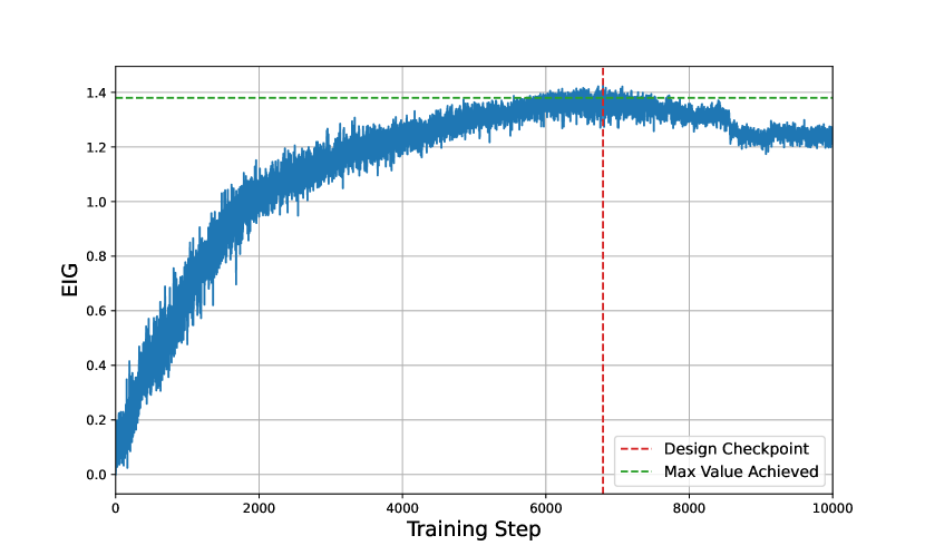
Figure 4: Training with design checkpoints saves an optimal design $\xi^{*}$ that achieves the highest EIG.

C.3 Design Checkpoints

Since designs and model parameters calculate the “reward” in the form of the EIG, it is possible that the EIG may fall into a local optima by the end of training. This may be because of decaying learning rates of the design gradients or decreasing area searched by the design distribution. We show an example in Figure˜4, where a global maximum is found earlier in training but ends in a local minima. We are assuming that it is better to use designs that achieve a global maximum EIG, which motivates the use of design checkpoints in our algorithm.

Appendix D Experiment Methodological Details

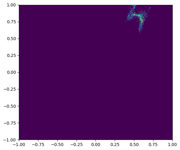
Figure 5: (Top) Posterior of the two moons experiments with mode collapse. (Bottom) Simulation-Based Calibration (SBC) of the posterior distribution for the two moons experiment.

For all experiments, we use a neural spline flow (NSF) normalizing flow. We specify the different parameterizations in Table 2. We used the ReduceLROnPlateau function to reduce the learning rate for the SIR and BMP experiments, whereas we used a constant learning rate for the linear experiment. We use the same learning rate for all flow parameters, $\phi$. Notably, for the iterated experimental design, we keep the previous round’s normalizing flow parameters, $\phi_{t-1}$ to use to return the subsequent round’s posterior. We set the Adam optimizer $\beta_{2}$ to be 0.95 to mitigate large jumps in $\xi$ that might destabilize training. All code is available online.

SIR Experiment Details

We follow the implementation of [Ivanova et al., 2021] for the SIR model. We solve an SDE describing the process using the Euler-Maruyama method and discretize the domain $\Delta\tau=10^{-2}$. The total population is fixed at $N=500$. For the model parameters $\beta$ and $\gamma$, we use log-normal priors such that $p(\beta)=\text{Lognorm}(0.50,0.50^{2})$ and $p(\gamma)=\text{Lognorm}(0.10,0.50^{2})$. Since solving the SDE is time-consuming, we pre-simulate data on a time grid in each round and access the relevant data regions during training.

BMP Experiment Details

The BMP signaling pathway can be described by mass action kinetics of proteins binding to one another and conservation laws to describe the process of a downstream genetic expression signal reaching a steady-state based on receptors available and ligands in a cell’s environment. The one-step model of BMP signaling was originally proposed by [Su et al., 2022]. While the model is described by an ODE in [Antebi et al., 2017], its steady-state signal is solved by convex optimization [Dirks et al., 2007] as a closed-box solver.

Appendix E Expanded Two Moons Results

We analyze the mode collapse of the likelihood-based two moons posterior prediction related to the MI optimization. We also show a Simulation-Based Calibration (SBC) [Talts et al., 2020, Hermans et al., 2022] curve for the two moons plot. For SBC we average over the parameters and compare the average posterior parameter values to the average prior values.

Mutual information optimization does not avoid mode collapse   Mode collapse in the two moons problem (Figure˜5) is a common issue when using a likelihood-based flow model. While we initially considered analyzing this through the lens of mutual information and its interpretation as the expected log ratio of the posterior to prior:

$$I(\theta;y)=\operatorname{{}\mathbb{E}}_{p(\theta,y)}\left[\log\frac{p(y|\theta)}{p(y)}\right]=\operatorname{{}\mathbb{E}}_{p(\theta,y)}\left[\log\frac{p(\theta|y)}{p(\theta)}\right],$$

our analysis in Section˜A.1 revealed that the root cause of mode collapse likely stems from deficiencies in the marginal likelihood approximation. There are two primary sources of error in the marginal likelihood estimation: the use of an approximate likelihood $p_{\phi}(y|\theta)$ and the reliance on finite samples to estimate the expectation. These approximations can introduce biases that may contribute to the observed mode collapse. Specifically, the InfoNCE bound used to maximize a lower bound of MI may be biased towards modes that better represent the observed data but potentially underrepresent the full range of parameter spaces that could explain the data.

Table 2: Training hyperparameters.

	Linear	SIR	BMP
Batch Size	10	256	128
Number of Contrastive Samples	50	255	127
Number of Gradient Steps	10000	10000	500
$\phi$ & $\xi$ Learning Rate	$1\times 10^{-3}$	$1\times 10^{-3}$	$1\times 10^{-3}$
Annealing Rate	NA	0.8	0.8
Final Learning Rate	NA	$1\times 10^{-4}$	$1\times 10^{-4}$
Gradient Clipping Threshold	NA	5	5
Hidden Layer Size	128	64	64
Number of Hidden Layers	4	2	2
Number of Flow layers (bijectors)	5	5	4
Number of bins for NSF	4	4	4

Indeed, [Foster et al., 2019] suggest simultaneously optimizing a posterior distribution at the same time as a likelihood via Likelihood-Free Adaptive Contrastive Estimation (LF-ACE). This approximates the marginal likelihood with a root sample from the prior $p(\theta_{0})$, and samples from an approximate posterior $\theta_{i}\sim q(\theta|y)$. This is essentially using samples from a posterior as importance sample estimates to help address the mode collapse of the approximate marginal likelihood. While theoretically sound, we attempted this using a normalizing flow to approximate and sample from the posterior. We found that training both the likelihood and posterior while optimizing designs to be unstable. Future work may address this with pretraining of one or both of the density estimators to improve stability of estimation.

SBI literature in accurate mutual information approximation [Miller et al., 2023, Glaser et al., 2022]while training amortized inference networks typically relies on using a generative model and critic in a similar form of importance sampling in a similar manner to LF-ACE. By addressing these issues in the marginal likelihood estimation, we may be able to develop more robust methods that avoid mode collapse in the two moons problem and related scenarios.

Appendix F Expanded BOED Results

Linear Model   We show the effect of varying design dimensions and $\lambda$ regularization on the EIG metric in Figure˜2. Optimizing a likelihood while optimizing experimental designs can struggle with high-dimensional designs but this is addressed with our regularization parameter.

SIR Model   The SIR model prior predictive distribution, true value, and subsequent posterior can be seen in Figure˜6 after $T=2$ experimental design rounds. We find a posterior approximation for this number of design rounds. We attempted to model the posterior when $T>2$ but found using the product likelihood identity of the likelihood using simple NUTS MCMC sampling in this regime challenging. This could be resolved with more sophisticated MCMC sampling methods such as Sequential Monte Carlo.

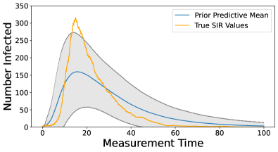
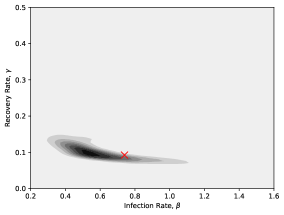
Figure 6: (Left) Prior predictive distributions for the SIR model with the true evaluation curve superimposed. (Middle) SIR posterior with true parameters at a red marker. (Right) SBC expected coverage curve indicating that the posterior is conservative, which agrees with a visual analysis of the current posterior.

BMP Model   The BMP model prior predictive and posterior distribution after $T=3$ rounds of experimental design in Figure˜7. We also found issues with MCMC sampling from the product likelihood in this case but our technique does show how to simultaneously optimize designs and a likelihood in a non-differentiable scientific simulator. However, we would like to be conservative in designing experiments as opposed to overconfident in a parameter inference to avoid designing experiments for the wrong hypotheses.

Improving Posterior Estimation   For both the SIR and BMP model, we only use a single round of inference for each round of BOED. All SBI algorithms can be refined by sequential application of drawing posterior samples conditioned on the observed data which will then help improve the quality of the likelihood [Papamakarios et al., 2019]. We forego this refinement step in our study in favor of examining how our method works with different settings of our regularization parameter. Depending on the simulator, this step can be computationally expensive but performing a calibration analysis of the likelihood can help to determine whether it is worth performing refinement steps.

Figure 7: (Left) Prior predictive distributions for the BMP model with the true evaluation curve superimposed and (Middle) its posterior with true parameters at a red marker. (Right) SBC expected coverage indcating a very conservative posterior, which is supported by the posterior in question. This posterior would likely benefit from multiple rounds of SBI due to the conservative posterior and the SBC expected coverage would indicate which round of SBI was most calibrated.

References

- Antebi et al. [2017] Y. E. Antebi, J. M. Linton, H. Klumpe, B. Bintu, M. Gong, C. Su, R. McCardell, and M. B. Elowitz. Combinatorial signal perception in the bmp pathway. Cell, 170(6):1184–1196, 2017.
- Ben-Hamu et al. [2024] H. Ben-Hamu, O. Puny, I. Gat, B. Karrer, U. Singer, and Y. Lipman. D-flow: Differentiating through flows for controlled generation. In Proceedings of the 41st International Conference on Machine Learning, volume 235 of Proceedings of Machine Learning Research, pages 3462–3483. PMLR, 21–27 Jul 2024.
- Bishop [1994] C. M. Bishop. Mixture density networks. 1994.
- Bradbury et al. [2018] J. Bradbury, R. Frostig, P. Hawkins, M. J. Johnson, C. Leary, D. Maclaurin, G. Necula, A. Paszke, J. VanderPlas, S. Wanderman-Milne, and Q. Zhang. JAX: composable transformations of Python+NumPy programs, 2018.
- Cranmer et al. [2020] K. Cranmer, J. Brehmer, and G. Louppe. The frontier of simulation-based inference. Proceedings of the National Academy of Sciences, 117(48):30055–30062, 2020.
- Devlin et al. [2019] J. Devlin, M.-W. Chang, K. Lee, and K. Toutanova. BERT: Pre-training of deep bidirectional transformers for language understanding. In Proceedings of the 2019 Conference of the North American Chapter of the Association for Computational Linguistics: Human Language Technologies, Volume 1 (Long and Short Papers), pages 4171–4186, June 2019.
- Dirks et al. [2007] R. M. Dirks, J. S. Bois, J. M. Schaeffer, E. Winfree, and N. A. Pierce. Thermodynamic analysis of interacting nucleic acid strands. SIAM review, 49(1):65–88, 2007.
- Durkan et al. [2019] C. Durkan, A. Bekasov, I. Murray, and G. Papamakarios. Neural spline flows. In H. Wallach, H. Larochelle, A. Beygelzimer, F. d'Alché-Buc, E. Fox, and R. Garnett, editors, Advances in Neural Information Processing Systems, volume 32. Curran Associates, Inc., 2019.
- Durkan et al. [2020] C. Durkan, I. Murray, and G. Papamakarios. On contrastive learning for likelihood-free inference. In Proceedings of the 37th International Conference on Machine Learning, volume 119 of Proceedings of Machine Learning Research, pages 2771–2781. PMLR, 13–18 Jul 2020.
- Foster et al. [2019] A. Foster, M. Jankowiak, E. Bingham, P. Horsfall, Y. W. Teh, T. Rainforth, and N. Goodman. Variational Bayesian optimal experimental design. Advances in Neural Information Processing Systems, Mar. 2019.
- Foster et al. [2020] A. Foster, M. Jankowiak, M. O’Meara, Y. W. Teh, and T. Rainforth. A unified stochastic gradient approach to designing bayesian-optimal experiments. In S. Chiappa and R. Calandra, editors, Proceedings of the Twenty Third International Conference on Artificial Intelligence and Statistics, volume 108 of Proceedings of Machine Learning Research, pages 2959–2969. PMLR, 26–28 Aug 2020.
- Foster et al. [2021] A. Foster, D. R. Ivanova, I. Malik, and T. Rainforth. Deep adaptive design: Amortizing sequential bayesian experimental design. In International conference on machine learning, pages 3384–3395. PMLR, 2021.
- Fujimoto et al. [2023] S. Fujimoto, W.-D. Chang, E. J. Smith, S. S. Gu, D. Precup, and D. Meger. For sale: State-action representation learning for deep reinforcement learning. In Proceedings of the 37th International Conference on Neural Information Processing Systems, 2023.
- Glaser et al. [2022] P. Glaser, M. Arbel, S. Hromadka, A. Doucet, and A. Gretton. Maximum likelihood learning of unnormalized models for simulation-based inference. arXiv preprint arXiv:2210.14756, 2022.
- Greenberg et al. [2019] D. Greenberg, M. Nonnenmacher, and J. Macke. Automatic posterior transformation for likelihood-free inference. In International Conference on Machine Learning, pages 2404–2414. PMLR, 2019.
- Hastie et al. [2009] T. Hastie, R. Tibshirani, J. H. Friedman, and J. H. Friedman. The elements of statistical learning: data mining, inference, and prediction, volume 2. Springer, 2009.
- Hermans et al. [2022] J. Hermans, A. Delaunoy, F. Rozet, A. Wehenkel, V. Begy, and G. Louppe. A crisis in simulation-based inference? beware, your posterior approximations can be unfaithful. Transactions on Machine Learning Research, 2022.
- Ho et al. [2020] J. Ho, A. Jain, and P. Abbeel. Denoising diffusion probabilistic models. In Proceedings of the 34th International Conference on Neural Information Processing Systems, 2020.
- Ivanova et al. [2021] D. R. Ivanova, A. Foster, S. Kleinegesse, M. U. Gutmann, and T. Rainforth. Implicit deep adaptive design: Policy-based experimental design without likelihoods. In Advances in Neural Information Processing Systems, volume 34, pages 25785–25798, 2021.
- Kleinegesse and Gutmann [2019] S. Kleinegesse and M. U. Gutmann. Efficient bayesian experimental design for implicit models. In The 22nd International Conference on Artificial Intelligence and Statistics, pages 476–485. PMLR, 2019.
- Kleinegesse and Gutmann [2020] S. Kleinegesse and M. U. Gutmann. Bayesian experimental design for implicit models by mutual information neural estimation. In Proceedings of the 37th International Conference on Machine Learning, volume 119, pages 5316–5326, 2020. arXiv: 2002.08129 Publication Title: arXiv.
- Kleinegesse and Gutmann [2021] S. Kleinegesse and M. U. Gutmann. Gradient-based Bayesian Experimental Design for Implicit Models using Mutual Information Lower Bounds. May 2021. arXiv: 2105.04379.
- Kobyzev et al. [2020] I. Kobyzev, S. Prince, and M. Brubaker. Normalizing Flows: An Introduction and Review of Current Methods. IEEE Transactions on Pattern Analysis and Machine Intelligence, Aug. 2020. ISSN 0162-8828.
- Lim et al. [2022] V. Lim, E. Novoseller, J. Ichnowski, H. Huang, and K. Goldberg. Policy-based bayesian experimental design for non-differentiable implicit models, 2022.
- Lin [1992] L.-J. Lin. Self-improving reactive agents based on reinforcement learning, planning and teaching. Machine learning, 8:293–321, 1992.
- Lindley [1956] D. V. Lindley. On a measure of the information provided by an experiment. The Annals of Mathematical Statistics, pages 986–1005, 1956.
- Lindley [1972] D. V. Lindley. Bayesian statistics, a review, volume 2. SIAM, 1972.
- Linhart et al. [2024] J. Linhart, A. Gramfort, and P. L. C. Rodrigues. L-c2st: Local diagnostics for posterior approximations in simulation-based inference. In Proceedings of the 37th International Conference on Neural Information Processing Systems, 2024.
- Lipman et al. [2023] Y. Lipman, R. T. Q. Chen, H. Ben-Hamu, M. Nickel, and M. Le. Flow matching for generative modeling. In Proceedings of the 11th International Conference on Learning Representations (ICLR), Kigali, Rwanda, 2023.
- Lueckmann et al. [2017] J.-M. Lueckmann, P. J. Goncalves, G. Bassetto, K. Öcal, M. Nonnenmacher, and J. H. Macke. Flexible statistical inference for mechanistic models of neural dynamics. Advances in neural information processing systems, 30, 2017.
- Lueckmann et al. [2021] J.-M. Lueckmann, J. Boelts, D. Greenberg, P. Goncalves, and J. Macke. Benchmarking simulation-based inference. In International Conference on Artificial Intelligence and Statistics, pages 343–351. PMLR, 2021.
- Miller et al. [2023] B. K. Miller, M. Federici, C. Weniger, and P. Forré. Simulation-based inference with the generalized kullback-leibler divergence. In 1st Workshop on the Synergy of Scientific and Machine Learning Modeling at ICML2023, 2023.
- Miller et al. [2024] B. K. Miller, C. Weniger, and P. Forré. Contrastive Neural Ratio Estimation. In Proceedings of the 36th International Conference on Neural Information Processing Systems, 2024.
- Mnih et al. [2013] V. Mnih, K. Kavukcuoglu, D. Silver, A. Graves, I. Antonoglou, D. Wierstra, and M. Riedmiller. Playing atari with deep reinforcement learning. In NIPS Deep Learning Workshop, 2013.
- Mohamed et al. [2020] S. Mohamed, M. Rosca, M. Figurnov, and A. Mnih. Monte carlo gradient estimation in machine learning. Journal of Machine Learning Research, 21(132):1–62, 2020.
- Nguyen et al. [2010] X. Nguyen, M. J. Wainwright, and M. I. Jordan. Estimating divergence functionals and the likelihood ratio by convex risk minimization. IEEE Transactions on Information Theory, 56(11):5847–5861, Nov. 2010. ISSN 1557-9654. doi: 10.1109/tit.2010.2068870.
- Papamakarios and Murray [2016] G. Papamakarios and I. Murray. Fast -free inference of simulation models with bayesian conditional density estimation. In Advances in Neural Information Processing Systems, volume 29, pages 1028–1036, 2016.
- Papamakarios et al. [2019] G. Papamakarios, D. C. Sterratt, and I. Murray. Sequential neural likelihood: Fast likelihood-free inference with autoregressive flows. In Proceedings of the 22nd International Conference on Artificial Intelligence and Statistics, pages 837–848. PMLR, 2019.
- Papamakarios et al. [2021] G. Papamakarios, E. Nalisnick, D. J. Rezende, S. Mohamed, and B. Lakshminarayanan. Normalizing flows for probabilistic modeling and inference. Journal of Machine Learning Research, 22(57):1–64, 2021.
- Paul et al. [2010] S. M. Paul, D. S. Mytelka, C. T. Dunwiddie, C. C. Persinger, B. H. Munos, S. R. Lindborg, and A. L. Schacht. How to improve r&d productivity: the pharmaceutical industry’s grand challenge. Nature reviews Drug discovery, 9(3):203–214, 2010.
- Poole et al. [2019] B. Poole, S. Ozair, A. Van Den Oord, A. Alemi, and G. Tucker. On variational bounds of mutual information. In International Conference on Machine Learning, pages 5171–5180. PMLR, 2019.
- Rainforth et al. [2018] T. Rainforth, R. Cornish, H. Yang, A. Warrington, and F. Wood. On nesting monte carlo estimators. In Proceedings of the 35th International Conference on Machine Learning, pages 4267–4276, 2018.
- Rezende and Mohamed [2015] D. J. Rezende and S. Mohamed. Variational inference with normalizing flows. In Proceedings of the 32nd International Conference on Machine Learning, pages 1530–1538. PMLR, 2015.
- Sisson et al. [2018] S. Sisson, Y. Fan, and M. Beaumont. Overview of approximate bayesian computation. arxiv e-prints, art. arXiv preprint arXiv:1802.09720, 2018.
- Song and Ermon [2020] J. Song and S. Ermon. Understanding the limitations of variational mutual information estimators. In International Conference on Learning Representations, 2020.
- Song and Ermon [2019] Y. Song and S. Ermon. Generative modeling by estimating gradients of the data distribution. In Proceedings of the 33rd International Conference on Neural Information Processing Systems, 2019.
- Song et al. [2022] Y. Song, C. Durkan, I. Murray, and S. Ermon. Maximum likelihood training of score-based diffusion models. In Proceedings of the 39th International Conference on Machine Learning, volume 162, pages 14429–14460, 2022.
- Su et al. [2022] C. J. Su, A. Murugan, J. M. Linton, A. Yeluri, J. Bois, H. Klumpe, M. A. Langley, Y. E. Antebi, and M. B. Elowitz. Ligand-receptor promiscuity enables cellular addressing. Cell systems, 13(5):408–425, 2022.
- Talts et al. [2020] S. Talts, M. Betancourt, D. Simpson, A. Vehtari, and A. Gelman. Validating bayesian inference algorithms with simulation-based calibration, 2020.
- van den Oord et al. [2019] A. van den Oord, Y. Li, and O. Vinyals. Representation learning with contrastive predictive coding, 2019.
- Vaswani et al. [2017] A. Vaswani, N. Shazeer, N. Parmar, J. Uszkoreit, L. Jones, A. N. Gomez, . Kaiser, and I. Polosukhin. Attention is all you need. Advances in neural information processing systems, 30, 2017.