Genuine multi-entropy and holography

Abstract

Is bipartite entanglement sufficient for holography? Through the analysis of the Markov gap Akers:2019gcv ; Hayden:2021gno , it is known that the answer is no. In this paper, we give a new perspective on this issue from a different angle using a multi-entropy Gadde:2022cqi ; Penington:2022dhr . We define a genuine $\mathtt{q}$-partite multi-entropy from a $\mathtt{q}$-partite multi-entropy by subtracting appropriate linear combinations of $\mathtt{\tilde{q}}$-partite multi-entropies for $\mathtt{\tilde{q}}<\mathtt{q}$, in such a way that the genuine $\mathtt{q}$-partite multi-entropy vanishes for all $\mathtt{\tilde{q}}$-partite entangled states. After studying several aspects, we apply it to black holes and holography. For the application to black holes, we see that such a genuine $\mathtt{q}$-partite multi-entropy is important only after the Page time. For the application to holography, we prove that non-bipartite multi-entropies are always positive and $\mathcal{O}\left({1/G_{N}}\right)$, as long as boundary subregions are connected. This indicates that for holography, genuine multi-partite entanglement is not small and plays an important role.

1 Introduction

Since the Ryu-Takayanagi (RT) formula Ryu:2006bv , which relates quantum entanglement entropy between boundary regions into minimal geometrical surfaces (RT-surface) in the bulk, was proposed, significant progress has been made in our understanding of holography from a quantum information viewpoint. Random tensor network (RTN) Hayden:2016cfa is one of such interesting development, which shows a very analogous formula to RT for the entanglement entropy and this analogy gives the view that RTN is a toy model of quantum gravity. Another interesting picture is given by a bit thread picture Freedman:2016zud , which gives a new perspective to the entanglement entropy as the maximum number of ‘bit threads’. Given that entanglement entropy is a bipartite measure, it is natural to ask if bipartite entanglement is enough for holography and it is conjectured that the entanglement of holographic CFT states is mostly bipartite (mostly-bipartite conjecture) in Cui:2018dyq .

In general quantum systems, one can divide the total system into three or more subsystems, and many states are involved in entanglement. In general, there is more than bipartite entanglement involved. For example, in spin systems, generic states contain more than bipartite entanglement, i.e., they contain genuine multi-partite entanglement such as tripartite and quadripartite entanglement. Famous examples of tripartite entanglement are the GHZ state and the W-state Dur:2000zz , which are distinguished from bipartite entangled states.

Even though the mostly-bipartite conjecture is quite interesting, it was disproved through the study of the Markov gap Akers:2019gcv ; Hayden:2021gno . Markov gap is defined as the difference between reflected entropy Dutta:2019gen and mutual information. The Markov gap is a useful quantity to detect genuine tripartite entanglement contribution in holography. Recently, another new multi-partite quantum entanglement measure has been proposed, which is called the multi-entropy Gadde:2022cqi ; Penington:2022dhr ; Gadde:2023zzj . In this paper, we would like to obtain a new perspective to the above-mentioned point by defining a genuine $\mathtt{q}$-partite multi-entropy using the multi-entropy. Here we point out the analogy between the Markov gap and genuine multi-entropy. Markov gap is defined using reflected entropy. On the other hand, genuine multi-entropy is defined using multi-entropy. We will see more of their analogy in detail.

The outline of this paper is as follows. In section 2, we define the genuine $\mathtt{q}$-partite multi-entropy for $\mathtt{q}=3$ case as a linear combination of the $\mathtt{q}=3$ and $\mathtt{q}=2$ multi-entropies. In section 3, we use this genuine $\mathtt{q}=3$ multi-entropy to study genuine tripartite entanglement in an evaporating black hole. The crucial approximation here is that we approximate an evaporating black hole and its radiation with a Haar-random state. Then we divide the total system into three subsystems, two for Hawking radiation subsystems and one for an evaporating black hole subsystem. By computing the genuine $\mathtt{q}=3$ multi-entropy in random states, we observe the time scale when the effect of genuine tripartite entanglement becomes large is always after the Page time. In section 4, we also apply the genuine multi-entropy in holography. We give a simple proof that non-bipartite entanglement is always positive and of order $\mathcal{O}(N^{2})=\mathcal{O}(1/G_{N})$ in holographic settings as far as the boundary subregions are connected. This explains why bipartite entanglement is not enough in holography, and this is similar to the nonnegative Markov gap Akers:2019gcv ; Hayden:2021gno . In this paper, we start a genuine $\mathtt{q}$-partite multi-entropy from $\mathtt{q}=3$ tripartite genuine case. However, one can also define genuine multi-entropy for $\mathtt{q}=4$ as well. In section 5, we discuss the genuine multi-entropy for $\mathtt{q}\geq 4$. We end in section 6 with open questions. Appendix A is for the maximum value of the genuine tri-partite multi-entropy in W-class, and Appendix B is for other measures constructed as products of bipartite measures. Note added: After writing the draft, we learned that part of the results in section 4 overlap with Harper:2024ker .

2 Defining a genuine multi-entropy in tripartite systems

In this section, we introduce the definition of multi-entropy and genuine tripartite multi-entropy by the linear combination of multi-entropies. Before we proceed, we first give our criterion for ‘genuineness’.

For that purpose, let us first consider a state that contains only bipartite entanglement. A typical example of such states is a triangle state $\ket{\Delta}_{ABC}$, which is defined in Zou:2020bly as

$$\ket{\Delta}_{ABC}=\ket{\psi}_{A_{R}B_{L}}\ket{\psi}_{B_{R}C_{L}}\ket{\psi}_{C_{R}A_{L}}\,,$$ (1)

See Fig. 1. Genuine tripartite entanglement measures must be zero for all of the triangle states. Later in section 2.2, we define the genuine tripartite multi-entropy, which we denote $GM^{(3)}(A:B:C)$, to satisfy this genuineness. In other words, our genuine tripartite multi-entropy, $GM^{(3)}(A:B:C)$, excludes all bipartite entanglement contributions.

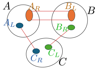
Figure 1: Triangle state is composed of bipartite entangled states only. Red lines represent bipartite entanglements.

The Markov gap, defined inAkers:2019gcv ; Hayden:2021gno also satisfies this criterion Zou:2020bly . One obvious difference between the Markov gap and our genuine tripartite multi-entropy is that the Markov gap is defined using a reflected entropy, on the other hand, the genuine tripartite multi-entropy is defined using a multi-entropy. Later we will comment more on their similarities and differences.

2.1 Multi-entropy in tripartite systems

Let us start with a review of multi-entropy and Rényi mutli-entropy. The Rényi mutli-entropy Gadde:2022cqi ; Penington:2022dhr ; Gadde:2023zzj was defined as a symmetric multi-partite entanglement measure in $\mathtt{q}$-partite systems. For instance, let us consider a tripartite pure state $|\psi\rangle$ on $\mathcal{H}=\mathcal{H}_{A}\otimes\mathcal{H}_{B}\otimes\mathcal{H}_{C}$. For such $\mathtt{q}=3$ tripartite systems, Rényi multi-entropy $S^{(3)}_{n}(A:B:C)$ of $|\psi\rangle$ is defined by

$$S^{(3)}_{n}(A:B:C) :=\frac{1}{1-n}\frac{1}{n}\log\frac{Z^{(3)}_{n}}{(Z^{(3)}_{1})^{n^{2}}},$$ (2)

$$Z^{(3)}_{n} :=\bra{\psi}^{\otimes n^{2}}\Sigma_{A}(g_{A})\Sigma_{B}(g_{B})\Sigma_{C}(g_{C})\ket{\psi}^{\otimes n^{2}},$$ (3)

where $\Sigma_{A,B,C}$ are the twist operators for the permutation action of $g_{A,B,C}$ on indices of density matrices. Their explicit representation of the permutation group is

$$g_{A} =(1,2,\dots,n)(n+1,n+2,\dots,2n)\cdots(n^{2}-n+1,n^{2}-n+2,\dots,n^{2}),$$ (4)

$$g_{B} =(1,n+1,\dots,n^{2}-n+1)(2,n+2,\dots,n^{2}-n+2)\cdots(n,2n,\dots,n^{2}),$$ (5)

$$g_{C} =(1)(2)\cdots(n^{2}).$$ (6)

See Fig. 2.

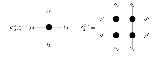
Figure 2: Contraction pattern of a reduced density matrix $\rho=\text{Tr}_{C}\ket{\psi}\bra{\psi}$ for $Z_{2}^{(3)}$.

The multi-entropy $S^{(3)}(A:B:C)$ is defined by

$$S^{(3)}(A:B:C):=\lim_{n\to 1}S^{(3)}_{n}(A:B:C).$$ (7)

The Rényi multi-entropy has the following properties Penington:2022dhr ; Gadde:2023zni .

• $S^{(3)}_{n}(A:B:C)$ is invariant under local unitary transformations of $|\psi\rangle$.

• $S^{(3)}_{n}(A:B:C)$ is symmetric in all the parties of tripartite systems:

  $$\;\;\;\;\;S^{(3)}_{n}(A:B:C)=S^{(3)}_{n}(A:C:B)=S^{(3)}_{n}(B:A:C)$$

  $$=S^{(3)}_{n}(B:C:A)=S^{(3)}_{n}(C:A:B)=S^{(3)}_{n}(C:B:A).$$ (8)

• $S^{(3)}_{n}(A:B:C)$ is additive under tensor products of pure states. If $|\psi\rangle_{A_{1}B_{1}C_{1}}$ and $|\phi\rangle_{A_{2}B_{2}C_{2}}$ are pure states, $S^{(3)}_{n}(A_{1}A_{2}:B_{1}B_{2}:C_{1}C_{2})_{|\psi\rangle\otimes|\phi\rangle}$ of $|\psi\rangle_{A_{1}B_{1}C_{1}}\otimes|\phi\rangle_{A_{2}B_{2}C_{2}}$ is given by

  $$\hskip-11.38109ptS^{(3)}_{n}(A_{1}A_{2}:B_{1}B_{2}:C_{1}C_{2})_{|\psi\rangle\otimes|\phi\rangle}=S^{(3)}_{n}(A_{1}:B_{1}:C_{1})_{|\psi\rangle}+S^{(3)}_{n}(A_{2}:B_{2}:C_{2})_{|\phi\rangle}.$$ (9)

These properties also hold for $(\mathtt{q},n)$-Rényi multi-entropy in $\mathtt{q}$-partite systems. As we will see soon, the additive property given by (9) plays an important role in defining genuine multi-entropy.

As concrete examples, we consider $S^{(3)}_{n}$ of W-state and GHZ state in three-qubit systems, where W-state and GHZ state Dur:2000zz are given by

$$|\text{GHZ}\rangle :=\frac{1}{\sqrt{2}}\left(|000\rangle+|111\rangle\right),$$ (10)

$$|\text{W}\rangle :=\frac{1}{\sqrt{3}}\left(|100\rangle+|010\rangle+|001\rangle\right).$$ (11)

For small $n=2,3,4$, $S^{(3)}_{n}$ of W-state is evaluated in Gadde:2022cqi but generic $n$ formula for Rényi multi-entropy is not known. They behave:

$$S^{(3)}_{2\;{|\text{W}\rangle}}=\frac{1}{2}\log 9=\log 3,$$ (12)

$$S^{(3)}_{3\;{|\text{W}\rangle}}=\frac{1}{6}\log\left(\frac{6561}{14}\right)\approx\frac{1}{6}\log\frac{3^{8}}{3^{2.4}}\approx 0.93\log 3,$$ (13)

$$S^{(3)}_{4\;{|\text{W}\rangle}}=\frac{1}{12}\log\left(\frac{14348907}{139}\right)\approx\frac{1}{12}\log\frac{3^{15}}{3^{4.5}}\approx{0.88}\log 3,\;$$ (14)

$$S^{(3)}_{5\;{|\text{W}\rangle}}=\frac{1}{20}\log\left(\frac{94143178827}{847}\right)\approx\frac{1}{20}\log\frac{3^{23}}{3^{6.1}}\approx 0.84\log 3,\;$$ (15)

$${S^{(3)}_{6\;{|\text{W}\rangle}}=\frac{1}{30}\log\left(\frac{50031545098999707}{87880}\right)\approx\frac{1}{30}\log\frac{3^{35}}{3^{10.4}}\approx 0.82\log 3.}\;$$ (16)

From these, we conjecture that

$$S^{3}_{1\;{|\text{W}\rangle}}=c_{\text{W}}\log 3\,,\quad\mbox{where $c_{\text{W}}>1$}\,.$$ (17)

On the other hand, for GHZ state, generic $n$ dependence for Rényi multi-entropy is known

$$S^{(3)}_{2\;{|\text{GHZ}\rangle}} =\frac{3}{2}\log 2,\;\quad\,\,\,\,S^{(3)}_{3\;{|\text{GHZ}\rangle}}=\frac{4}{3}\log 2,\;\quad\,\,\,\,S^{(3)}_{4\;{|\text{GHZ}\rangle}}=\frac{5}{4}\log 2,$$ (18)

$$S^{(3)}_{n\;{|\text{GHZ}\rangle}} =\frac{1+n}{n}\log 2,\;\,\,\,S^{(3)}_{{|\text{GHZ}\rangle}}=2\log 2.$$ (19)

As another example, consider a triangle state $\ket{\Delta}$ given by (1), which has no genuine tripartite entanglement. For such a triangle state, its Rényi multi-entropy $S^{(3)}_{n}(A:B:C)_{|\Delta\rangle}$ satisfies the following relationship Penington:2022dhr

$$S^{(3)}_{n}(A:B:C)_{|\Delta\rangle}=\frac{1}{2}\left(S_{n}^{(2)}(A)_{|\Delta\rangle}+S_{n}^{(2)}(B)_{|\Delta\rangle}+S_{n}^{(2)}(C)_{|\Delta\rangle}\right),$$ (20)

where

$$S_{n}^{(2)}(A)_{|\Delta\rangle}:=\frac{1}{1-n}\log\text{Tr}_{A}\rho_{A}^{n}$$ (21)

is a Rényi entanglement entropy for reduced density matrix $\rho_{A}:=\text{Tr}_{BC}|\Delta\rangle\langle\Delta|$. Thus, we also write $S_{n}^{(2)}(A:BC)=S_{n}^{(2)}(A)$, $S_{n}^{(2)}(B:CA)=S_{n}^{(2)}(B)$, $S_{n}^{(2)}(C:AB)=S_{n}^{(2)}(C)$. In particular, for three-qubit systems $A$, $B$, $C$, we obtain

$$S^{(3)}_{n}(A:B:C)_{|\Delta\rangle}\leq\log 2,$$ (22)

which is smaller than $S^{(3)}_{n\;{|\text{GHZ}\rangle}}$ if $n>0$.

By comparing (16) and (18), one can see that $S^{(3)}_{n\;{|\text{W}\rangle}}$ is larger than $S^{(3)}_{n\;{|\text{GHZ}\rangle}}$ in the calculation examples above for $n\geq 2$. In addition, our numerical computations imply that $S^{(3)}_{2\;{|\text{W}\rangle}}$ is maximum among $S^{(3)}_{2}$ in three qubit systems. As a partial proof, in Appendix A, we show that $S^{(3)}_{2\;{|\text{W}\rangle}}$ is maximum among $S^{(3)}_{2}$ in W-class. Therefore, we conjecture that $S^{(3)}_{n\;{|\text{W}\rangle}}$ is maximum among $S^{(3)}_{n}$ in three qubit systems.

2.2 Genuine multi-entropy in tripartite systems

Generally, $S^{(3)}_{n}$ is nonzero for pure states with bipartite entanglement as seen in (20). In tripartite systems, there are two types of entanglement: bipartite entanglement between two subsystems and genuine tripartite entanglement between three subsystems Dur:2000zz .

For generic $\mathtt{q}$, we define a genuine $\mathtt{q}$-partite multi-entropy from a $\mathtt{q}$-partite multi-entropy by subtracting appropriate linear combinations of $\mathtt{\tilde{q}}$-partite multi-entropies for $\mathtt{\tilde{q}}<\mathtt{q}$, in such a way that the genuine $\mathtt{q}$-partite multi-entropy vanish for all $\mathtt{\tilde{q}}$-partite entangled states. Thus, for $\mathtt{q}=3$ case, we define the genuine multi-entropy in such a way that it gives zero for pure states with only bipartite entanglement. Then the following linear combination works,

$$GM_{n}^{(3)}(A:B:C) :=S^{(3)}_{n}(A:B:C)-\frac{1}{2}\left(S_{n}^{(2)}(A:BC)+S_{n}^{(2)}(B:CA)+S_{n}^{(2)}(C:AB)\right).$$ (23)

From (20), it immediately follows that $GM_{n}^{(3)}(A:B:C)$ of the triangle state $|\Delta\rangle$, which has only bipartite entanglement, is zero. We call $GM_{n}^{(3)}(A:B:C)$ genuine $n$-th Rényi multi-entropy $(\mathtt{q}=3)$ in tripartite systems. As an independent work from us, in Liu:2024ulq the same quantity (23) is defined as $\kappa_{n}$ and values on 2d CFTs are studied.

We define the genuine $\mathtt{q}=3$ multi-entropy $GM^{(3)}(A:B:C)$ by taking the $n\to 1$ limit as

$$GM^{(3)}(A:B:C):=\lim_{n\to 1}GM_{n}^{(3)}(A:B:C).$$ (24)

Later in section 4, we prove that

$$GM^{(3)}(A:B:C)\geq 0$$ (25)

using holographic duals.

The Rényi $n=2$ case is interesting as well since in this case, the multi-entropy $S^{(3)}_{n=2}(A:B:C)$ essentially reduces to the reflected entropy. See Figure 13 of Iizuka:2024pzm for the four replica contraction diagram. In this case, one can show that the genuine $n=2$ Rényi multi-entropy $(\mathtt{q}=3)$ is related to the Rényi Markov gap, which is the difference between the Rényi reflected entropy and the Rényi mutual entropy, as Liu:2024ulq

$$GM_{n=2}^{(3)}(A:B:C)\propto\mbox{(($m=2,n=2$) R\'{e}nyi Markov gap)}.$$ (26)

We will comment on this relation more in detail in the next section.

Note that both the Markov gap and the genuine multi-entropy $\mathtt{q}=3$ vanish for the states containing only bipartite entanglement. Thus for $\mathtt{q}=3$ tripartite case, their properties are expected to be similar in general. Next, we will comment on properties of the genuine $\mathtt{q}=3$ multi-entropy through explicit examples.

For W-state, one can obtain $GM_{n}^{(3)}$ for small $n$ as follows,

$$GM^{(3)}_{2\;{|\text{W}\rangle}} =\log\left(\frac{5\sqrt{5}}{9}\right),\;\qquad\quad\,\,\,GM^{(3)}_{3\;{|\text{W}\rangle}}=\frac{1}{12}\log\left(\frac{2187}{196}\right),\;$$ (27)

$$GM^{(3)}_{4\;{|\text{W}\rangle}} =\frac{1}{12}\log\left(\frac{24137569}{2735937}\right),\;\,GM^{(3)}_{5\;{|\text{W}\rangle}}=\frac{1}{40}\log\left(\frac{285311670611}{234365481}\right),$$ (28)

$${GM^{(3)}_{6\;{|\text{W}\rangle}}} =\frac{1}{120}\log\left(\frac{72890483685103052142902866787761839379440139451}{725120831374733747546618320576719360000}\right),$$ (29)

using

$$S^{(2)}_{n\;{|\text{W}\rangle}} =\frac{\log\left(\left(2^{n}+1\right)/3^{n}\right)}{1-n}\,,\quad\mbox{with}\quad S^{(2)}_{\;{|\text{W}\rangle}}=\log 3-\frac{2}{3}\log 2\,.$$ (30)

All of $GM_{n}^{(3)}$ for $n=2,3,4,5,6$ are positive. Finally using (17) and (30), for $n\to 1$ case we have

$$GM^{(3)}_{\;{|\text{W}\rangle}} =\log\left(2\,3^{c_{W}-\frac{3}{2}}\right)>\log\left(2\,3^{-\frac{1}{2}}\right)\approx 0.14>0\quad\mbox{for $c_{W}>1$.}$$ (31)

In contrast, $GM^{(3)}_{n}$ of GHZ state is Liu:2024ulq

$$GM^{(3)}_{n\;{|\text{GHZ}\rangle}} =\left(\frac{1+n}{n}-\frac{3}{2}\right)\log 2.\,$$ (32)

Especially this means for $n\to 1$ and $n\to 2$ cases,

$$GM^{(3)}_{{|\text{GHZ}\rangle}} =\frac{1}{2}\log 2>0\,\quad(n\to 1)$$ (33)

$$GM^{(3)}_{2\;{|\text{GHZ}\rangle}} =0\quad(n\to 2),$$ (34)

where genuine multi-entropy $GM^{(3)}_{{|\text{GHZ}\rangle}}$ is positive, but $GM^{(3)}_{n\;{|\text{GHZ}\rangle}}$ is negative if $n>2$. Thus, even though $GM^{(3)}$ is expected to behave similarly to Markov gap Hayden:2021gno , there are important differences. One difference between Markov gap and genuine multi-entropy $GM^{(3)}$ is that Markov gap of GHZ state is zero, but $GM^{(3)}$ of GHZ state is nonzero as (33). This means that the Markov gap cannot capture genuine tripartite entanglement in the GHZ state, on the other hand, $GM^{(3)}$ can capture it. Another note is that even though we have not yet proved it, it is likely that $c_{W}>1$ in (17) from (12) - (16). This implies that for both GHZ state and W state, $GM^{(3)}>0$ as (31) and (33). This inequality is the same as (25), however the origin is totally different since there is no guarantee that GHZ state or W state can be holographic.

So far, we focus on $\mathtt{q}=3$ tripartite case. However similarly it is possible to define genuine multi-entropy for higher $\mathtt{q}$ cases as well, using the same principles. We will comment on this in Section 5.

Other than the simple spin systems, several papers studied 2d CFT cases as in Penington:2022dhr ; Gadde:2023zzj ; Harper:2024ker . In particular, $GM^{(3)}_{n}(A:B:C)$ in 2d CFTs and a free fermion model on a 2d square lattice was studied in Liu:2024ulq . See also Yuan:2024yfg ; Gadde:2024taa for 2d CFT computations for some generalizations of the multi-entropy.

Before we proceed, we comment on other proposal for the genuine multi-partite entanglement. One of such proposal is the ‘L-entropy’ defined by Basak:2024uwc . The bipartite L-entropy $l_{AB}$ was defined as

$$l_{AB}:=\text{Min}\{2S^{(2)}(A),2S^{(2)}(B)\}-S^{(1,1)}_{R}(A:B),$$ (35)

which is motivated by the inequality $S^{(1,1)}_{R}(A:B)\leq\text{Min}\{2S^{(2)}(A),2S^{(2)}(B)\}$, just as the Markov gap was motivated by the inequality $I^{(1)}(A:B)\leq S^{(1,1)}_{R}(A:B)$. The tripartite L-entropy is a product of three bipartite L-entropies, namely $l_{AB},l_{BC},l_{CA}$. However, the L-entropy does not satisfy the additive property (9) due to

$$\text{Min}\{S^{(2)}(A_{1}),S^{(2)}(B_{1})\}+\text{Min}\{S^{(2)}(A_{2}),S^{(2)}(B_{2})\}$$

$$\neq\text{Min}\{S^{(2)}(A_{1})+S^{(2)}(A_{2}),S^{(2)}(B_{1})+S^{(2)}(B_{2})\}.$$ (36)

The lack of additive property is crucial since this leads to the property that L-entropy does not vanish for the triangle state (1). Thus L-entropy does not measure the genuine tripartite entanglement in our criteria.

3 Black hole genuine multi-entropy curve

As an application of the multi-entropy to a black hole evaporation, the black hole multi-entropy curve was introduced and studied by Iizuka:2024pzm . This is a natural generalization of the Page curve of entanglement entropy. The crucial point is that we approximate an evaporating black hole and its radiation with a Haar-random state for this purpose. In this section, similarly to the previous work, we study the genuine multi-entropy $GM^{(3)}(A:B:C)$ curve for the following tripartite systems: two Hawking radiation subsystems $A=\text{R1}$ and $B=\text{R2}$, and an evaporating black hole subsystem $C=\text{BH}$.

More concretely, we first compute the black hole genuine $n=2$ Rényi tripartite entropy curve of $GM_{2}^{(3)}(\text{R1}:\text{R2}:\text{BH})$ by using a single random tensor model as in the original work of Page curve Page:1993df ; Page:1993wv . The explicit expressions of Rényi multi-entropy are given by Iizuka:2024pzm

$$S^{(3)}_{2}(\text{R1}:\text{R2}:\text{BH})=-\frac{1}{2}\log\left[\frac{d_{\rm R}^{2}d_{\rm BH}(9+2d_{\rm R}^{2}+d_{\rm BH}^{2})+2(2d_{\rm R}^{2}+d_{\rm BH}^{2}+d_{\rm R}^{4}+2d_{\rm R}^{2}d_{\rm BH}^{2})}{(1+d_{\rm BH}d_{\rm R}^{2})(2+d_{\rm BH}d_{\rm R}^{2})(3+d_{\rm BH}d_{\rm R}^{2})}\right],$$ (37)

$$\quad S^{(2)}_{2}(\text{R1})=S^{(2)}_{2}(\text{R2})=-\log\left[\frac{d_{\rm R}+d_{\rm R}d_{\rm BH}}{1+d_{\rm BH}d_{\rm R}^{2}}\right],\;\quad S^{(2)}_{2}(\text{BH})=-\log\left[\frac{d_{\rm BH}+d_{\rm R}^{2}}{1+d_{\rm BH}d_{\rm R}^{2}}\right],$$ (38)

where we set $\dim\mathcal{H}_{\text{R1}}=\dim\mathcal{H}_{\text{R2}}=d_{\text{R}}$ and $\dim\mathcal{H}_{\text{BH}}=d_{\text{BH}}$. We also fix the dimension of total system

$$d_{\rm Total}=d_{\rm BH}d_{\rm R}^{2}\mbox{ = fixed}.$$ (39)

By using $d_{\rm BH}=d_{\rm Total}/d_{\rm R}^{2}$, we can plot $GM_{2}^{(3)}(\text{R1}:\text{R2}:\text{BH})$ as a function of $d_{\rm R}$.

Figure 3 shows the black hole genuine $\mathtt{q}=3,n=2$ Rényi multi-entropy curve of $GM_{2}^{(3)}(\text{R1}:\text{R2}:\text{BH})$. The black curve shows $GM_{2}^{(3)}(\text{R1}:\text{R2}:\text{BH})$ with $d_{\rm Total}=10^{12}$, where the horizontal axis is $\log d_{\text{R}}$. In the black hole $\mathtt{q}=3$ Rényi multi-entropy curve, there are only one time scale, which is the multi-entropy time

$$d_{\rm R}=d_{\rm BH}=d_{\rm Total}/d_{\rm R}^{2}\quad \Leftrightarrow\quad d_{\rm R}=\left(d_{\rm Total}\right)^{1/3}\quad\mbox{(Multi-entropy time)}.$$ (40)

For bipartite entanglement entropy, there is only one time scale, which is the Page time

$$d_{\rm R}^{2}=d_{\rm BH}=d_{\rm Total}/d_{\rm R}^{2}\quad \Leftrightarrow\quad d_{\rm R}=\left(d_{\rm Total}\right)^{1/4}\quad\mbox{(Page time)}$$ (41)

Since $\mathtt{q}=3$ genuine multi-entropy is a linear combination of $\mathtt{q}=3$ and $\mathtt{q}=2$ multi-entropies, there are only two time scales for that, and one can see this in Fig. 3.

The black hole genuine $n=2$ Rényi multi-entropy curve of $GM_{2}^{(3)}(\text{R1}:\text{R2}:\text{BH})$ is initially zero and starts to increase after the Page time. Then, $GM_{2}^{(3)}(\text{R1}:\text{R2}:\text{BH})$ starts to decrease from the multi-entropy time, and finally vanishes. In particular, we can see that the genuine $n=2$ Rényi multi-entropy $GM_{2}^{(3)}(\text{R1}:\text{R2}:\text{BH})$ becomes nonzero and large only after the Page time. Thus, the Page time determines the time scale when it deviates from zero, and the multi-entropy time determines the time scale when it reaches maximum.

For the comparison of the magnitudes, we also plot the Page curve of $S^{(2)}_{2}(\text{BH})$ by the blue curve, which initially increases and starts to decrease from the Page time. One can see that even though the genuine tripartite multi-entropy contribution is smaller than the bipartite entanglement entropy, their magnitudes are similar in order. This implies that the genuine multi-partite entanglement is not small.

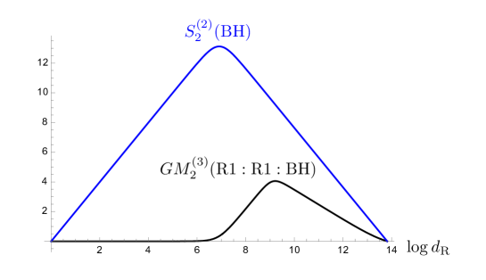
Figure 3: Black curve: black hole Rényi multi-entropy curve of $GM_{2}^{(3)}(\text{R1}:\text{R2}:\text{BH})$. Blue curve: Page curve of $S^{(2)}_{2}(\text{BH})$. We fix the total dimension $d_{\rm Total}=d_{\rm BH}d_{\rm R}^{2}=10^{12}$.

Next, we study $n\to 1$ limit. The asymptotic behaviors of $S^{(3)}_{n}(\text{R1}:\text{R2}:\text{BH})$ at $d_{\text{R}}\ll d_{\text{BH}}$ and $d_{\text{R}}\gg d_{\text{BH}}$ was studied by Iizuka:2024pzm . By using these expressions, we can plot the asymptotic behaviors in the black hole genuine multi-entropy curve of $GM^{(3)}(\text{R1}:\text{R2}:\text{BH})$ at $n\to 1$. Figure 4 shows the asymptotic behaviors of $GM^{(3)}(\text{R1}:\text{R2}:\text{BH})$ and $S^{(2)}_{1}(\text{BH})$. Since these are only the asymptotic behaviors, these plots are not smooth at the Page time and the multi-entropy time. Comparing Figures 3 and 4, one can see that the qualitative behavior of $GM_{n}^{(3)}(\text{R1}:\text{R2}:\text{BH})$ is independent of $n$. This is due to the fact that the asymptotic behaviors (5.23) in Iizuka:2024pzm is not sensitive to $n$ if we divide them by a factor $n^{\mathtt{q}-2}$ as explained in footnote 2. In particular, the two time scales, the Page time and the multi-entropy time, do not depend on $n$.

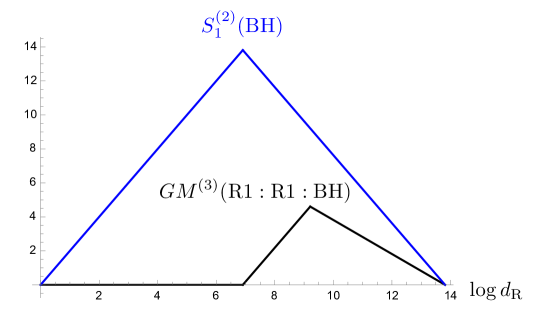
Figure 4: Asymptotic behaviors of $GM^{(3)}(\text{R1}:\text{R2}:\text{BH})$ and $S^{(2)}_{n\to 1}(\text{BH})$.

We also plot a similar curve of the Markov gap by using the study of reflected entropy in a single random tensor model by Akers:2021pvd . Rényi generalization of Markov gap $h^{m,n}(A:B)$ is defined by Sohal:2023hst ; Berthiere:2023gkx ; Liu:2024ulq

$$h^{m,n}(A:B):=S_{R}^{(m,n)}(A:B)-I^{(n)}(A:B),$$ (42)

where $I^{(n)}(A:B):=S_{n}^{(2)}(A)+S_{n}^{(2)}(B)-S_{n}^{(2)}(AB)$ is Rényi mutual information, and $S_{R}^{(m,n)}(A:B)$ is Rényi reflected entropy defined in Dutta:2019gen as

$$S_{R}^{(m,n)}(A:B) :=\frac{1}{1-n}\log\frac{Z_{m,n}}{(Z_{m,1})^{n}},$$ (43)

$$Z_{m,n} :=\Tr_{AA^{*}}\left(\Tr_{BB^{*}}|\rho_{AB}^{m/2}\rangle\langle\rho_{AB}^{m/2}|\right)^{n},$$ (44)

where $|\rho_{AB}^{m/2}\rangle$ is the canonical purified state of $\rho_{AB}^{m}$. Markov gap $h$ is defined by

$$h:=\lim_{m\to 1}\lim_{n\to 1}h^{m,n}(A:B).$$ (45)

Here, the reduced density matrix $\rho_{AB}$ is defined by

$$\rho_{AB}:=\text{Tr}_{C}|\psi\rangle\langle\psi|,$$ (46)

for a given pure state $|\psi\rangle$ on $\mathcal{H}_{A}\otimes\mathcal{H}_{B}\otimes\mathcal{H}_{C}$. The explicit expression of $S_{R}^{(2,2)}(\text{R1}:\text{R2})$ for a random state $|\psi\rangle$ on $\mathcal{H}_{\text{R1}}\otimes\mathcal{H}_{\text{R2}}\otimes\mathcal{H}_{\text{BH}}$ is Iizuka:2024pzm

$$S_{R}^{(2,2)}(\text{R1}:\text{R2})=-\log\frac{d_{\rm R}^{2}d_{\rm BH}(9+2d_{\rm R}^{2}+d_{\rm BH}^{2})+2(2d_{\rm R}^{2}+d_{\rm BH}^{2}+d_{\rm R}^{4}+2d_{\rm R}^{2}d_{\rm BH}^{2})}{d_{\text{BH}}^{3}d_{\text{R}}^{2}+d_{\text{BH}}^{2}(2d_{\text{R}}^{4}+4)+d_{\text{BH}}(d_{\text{R}}^{6}+10d_{\text{R}}^{2})+4d_{\text{R}}^{4}+2},$$ (47)

where we set $\dim\mathcal{H}_{\text{R1}}=\dim\mathcal{H}_{\text{R2}}=d_{\text{R}}$ and $\dim\mathcal{H}_{\text{BH}}=d_{\text{BH}}$.

Figure 5 shows a curve of $h^{2,2}(\text{R1}:\text{R2})$ with the fixed total dimension $d_{\rm Total}=d_{\rm BH}d_{\rm R}^{2}=10^{12}$. This plot has a similar behavior to $GM_{2}^{(3)}(\text{R1}:\text{R2}:\text{BH})$ in Figure 3. In fact, there is a relation between $GM_{2}^{(3)}(A:B:C)$ and $h^{2,2}(A:B)$ Liu:2024ulq

$$GM_{2}^{(3)}(A:B:C)=\frac{1}{2}\,{h^{2,2}(A:B)}.$$ (48)

One difference between $GM_{n}^{(3)}(\text{R1}:\text{R2}:\text{BH})$ and $h^{m,n}(\text{R1}:\text{R2})$ is that the time scale of $h^{m,n}(\text{R1}:\text{R2})$ to start decreasing depends on $n$. From the result (3.96) in Akers:2021pvd , this time scale of $h^{1,n}(\text{R1}:\text{R2})$ is given by

$$d_{\rm R}^{2/n}=d_{\rm BH}=d_{\rm Total}/d_{\rm R}^{2}\quad \Leftrightarrow\quad d_{\rm R}=\left(d_{\rm Total}\right)^{\frac{n}{2(1+n)}},$$ (49)

which coincides the Page time when $n\to 1$. Therefore, there is the transition in the asymptotic behavior of the Markov gap $h(\text{R1}:\text{R2})$ at the Page time as shown in Figure 6.

Figure 5: Curve of $h^{2,2}(\text{R1}:\text{R2})$ with the total dimension $d_{\rm Total}=d_{\rm BH}d_{\rm R}^{2}=10^{12}$.

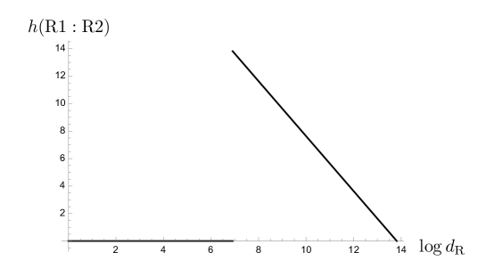
Figure 6: Asymptotic behavior of Markov gap $h(\text{R1}:\text{R2})$. There is the transition of asymptotic behavior at the Page time.

Before we end, we summarize the characteristic natures of these curves.

1. It is always only after the Page time, this genuine multi-entropy becomes large. This means before the Page time, essentially there is no contribution by genuine tripartite multi-entropy, compared with the bipartite entanglement.

2. As Fig. 3 and Fig. 4 show, after the Page time, the amount of genuine tripartite multi-entropy is not parametrically small compared with the bipartite entanglement.

3. The genuine $\mathtt{q}=3$ multi-entropy curve Fig. 4 shows the peak at the multi-entropy time. On the other hand, the Markov gap Fig. 6 shows the peak at the Page time. Even though both capture the genuine tripartite entanglement, the peak is at different time scales. This is because they are different measures. Note that a multi-entropy treats all subsystems on equal footing, however, the Markov gap does not. However, both quantities show nonzero value only after the Page time.

Quite interestingly, the L-entropy Basak:2024uwc also shows a very similar curve. See their Figure 17. However, as we commented before, since L-entropy does not vanish for the triangle state, their contributions is not necessary for genuine tripartite entanglement. In fact, quite similar curve can be obtained from the products of logarithmic negativity, see Appendix B for more detail. It is interesting to investigate the difference between L-entropy and genuine multi-partite quantities in detail and see why Figure 17 of Basak:2024uwc and Figure 3 are similar.

4 Why bipartite entanglement is not enough for holography

In this section, we show the inequality (25) for $GM^{(3)}(A:B:C)$ holds in holographic settings. The proof is very simple. To show this, let’s divide the boundary space into three regions/subsystems and let us call them $A$, $B$, $C$ respectively. The holographic multi-entropy $S^{(3)}(A:B:C)$ is given by the sum of the three surfaces, $\gamma_{xo}$, $\gamma_{yo}$ and $\gamma_{zo}$ Gadde:2022cqi ; Gadde:2023zzj , as

$$S^{(3)}(A:B:C)=\frac{1}{4G_{N}}\left(\gamma_{xo}+\gamma_{yo}+\gamma_{zo}\right)$$ (50)

where $O$ is their meeting point. See the left figure of Fig. 7. In this section, we assume that holographic multi-entropy is given by the formula as (50).

On the other hand, the entanglement entropy $S_{A}$, $S_{B}$, $S_{C}$ are given by the RT-surfaces $\gamma_{A}$, $\gamma_{B}$, $\gamma_{C}$ Ryu:2006bv . Thus,

$$S_{A}+S_{B}+S_{C}=\frac{1}{4G_{N}}\left(\gamma_{A}+\gamma_{B}+\gamma_{C}\right)$$ (51)

See the right figure of Fig. 7.

Thus, the genuine multi-entropy is always non-negative

$$S^{(3)}(A:B:C)-\frac{1}{2}\left(S_{A}+S_{B}+S_{C}\right)$$

$$\,\,=\frac{1}{8G_{N}}\left(\gamma_{xo}+\gamma_{yo}-\gamma_{A}\right)+\frac{1}{8G_{N}}\left(\gamma_{yo}+\gamma_{zo}-\gamma_{B}\right)+\frac{1}{8G_{N}}\left(\gamma_{zo}+\gamma_{xo}-\gamma_{C}\right)>0$$ (52)

since each parenthesis is always positive because RT-surfaces $\gamma_{A}$, $\gamma_{B}$, $\gamma_{C}$ are minimal surfaces. See Fig. 8. The similar proof is also shown in Harper:2024ker .

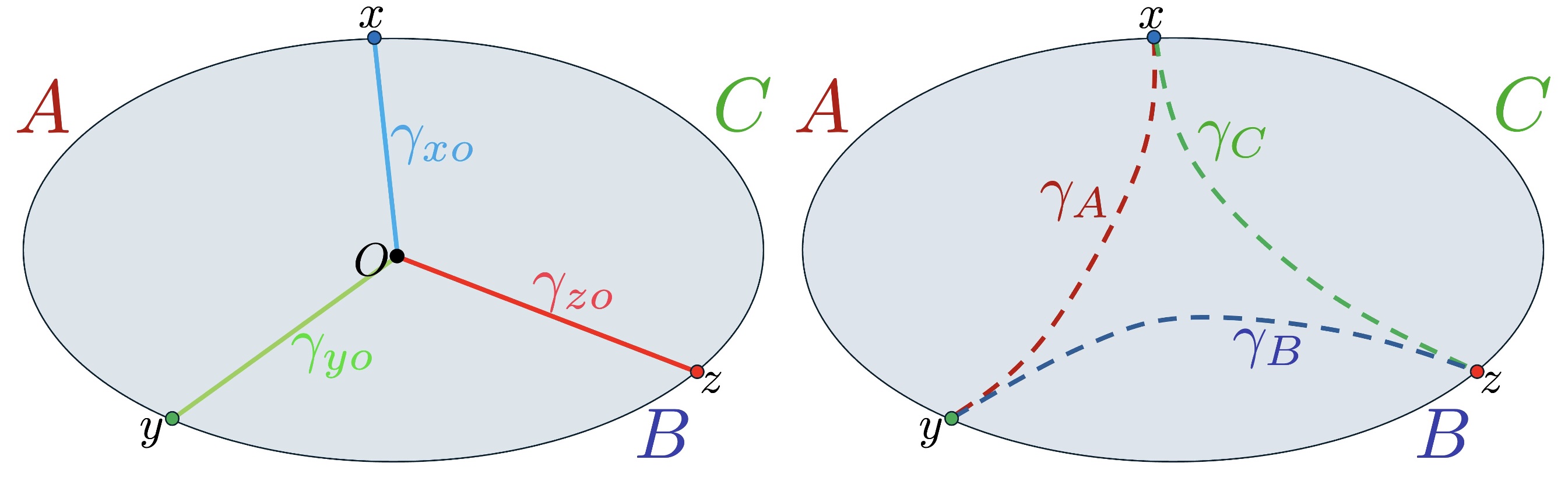
Figure 7: Left: Holographic multi-entropy is given by the sum of the three surfaces, $\gamma_{xo}$, $\gamma_{yo}$ and $\gamma_{zo}$. Right: RT surfaces $\gamma_{A}$, $\gamma_{B}$, $\gamma_{C}$ for the entanglement entropy $S_{A}$, $S_{B}$, $S_{C}$.

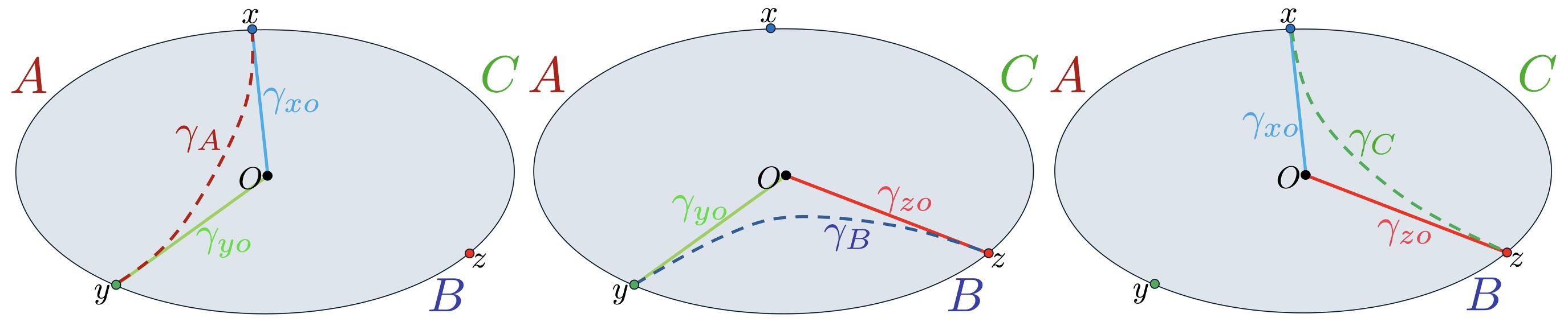
Figure 8: The genuine multi-entropy $\mathtt{q}=3$ reduces to the subtraction of 3 minimal surfaces. However, due to the fact that $\gamma_{A}$, $\gamma_{B}$, $\gamma_{C}$ are minimal surfaces, each parenthesis in (4) is always positive quantities. Thus genuine multi-entropy is positive.

This holographic proof is analogous to the one given for the Markov gap given by Hayden:2021gno . See their Fig. 3. In this way, even holographic-wise, genuine multi-entropy and the Markov gap share some similarities. However, there are also several differences. We summarize their analogies and differences here.

1. Both the Markov gap and genuine multi-entropy are measures for genuine multi-partite entanglement in the sense that both quantities vanish for bipartite entangled states.

2. However for GHZ state, which is one of the genuine multi-partite states, there is a difference. The Markov gap vanishes for the GHZ state, on the other hand, genuine multi-entropy gives a positive value for the GHZ state.

3. Markov gap is defined for tripartite states in the sense that the reflected entropy is defined by tracing $C$ and leaving only subsystems $A$ and $B$. There is no way to furthermore divide the subsystem $C$ into finer subsystems. On the other hand, since the multi-entropy is defined in generic $\mathtt{q}$-partite system, it is possible to define a genuine multi-entropy even for $\mathtt{q}\geq 4$ case as well. We will comment on this in more detail later in the next section.

In this way, both the genuine multi-entropy and the Markov gap give evidence that in holography genuine tripartite entanglement is not small.

So far, we have focused on the $\mathtt{q}=3$ case. However, this proof can be easily generalized for higher $\mathtt{q}$ as well. The $n$-th Rényi multi-entropy of a pure state $\ket{\psi}$ on $\mathtt{q}$-partite subsystems $A_{1},A_{2},\dots,A_{\mathtt{q}}$ is defined by Gadde:2022cqi ; Gadde:2023zzj ; Gadde:2023zni

$$S^{(\mathtt{q})}_{n}(A_{1}:A_{2}:\cdots:A_{\mathtt{q}}) :=\frac{1}{1-n}\frac{1}{n^{\mathtt{q}-2}}\log\frac{Z^{(\mathtt{q})}_{n}}{(Z^{(\mathtt{q})}_{1})^{n^{\mathtt{q}-1}}},$$ (53)

$$Z^{(\mathtt{q})}_{n} :=\bra{\psi}^{\otimes n^{\mathtt{q}-1}}\Sigma_{1}(g_{1})\Sigma_{2}(g_{2})\cdots\Sigma_{\mathtt{q}}(g_{\mathtt{q}})\ket{\psi}^{\otimes n^{\mathtt{q}-1}},$$ (54)

where $\Sigma_{k}(g_{k})$ are twist operators for the permutation action of $g_{k}$ on indices of density matrices for $A_{k}$. The action of $g_{k}$ can be expressed as

$$g_{k} \cdot(x_{1},\cdots,x_{k},\cdots,x_{\mathtt{q}-1})=(x_{1},\cdots,x_{k}+1,\cdots,x_{\mathtt{q}-1}),\quad 1\leq k\leq\mathtt{q}-1,$$ (55)

$$g_{\mathtt{q}} =e,$$ (56)

where $(x_{1},x_{2},\cdots,x_{\mathtt{q}-1})$ represents an integer lattice point on a $(\mathtt{q}-1)$-dimensional hypercube of length $n$, and we identify $x_{k}=n+1$ with $x_{k}=1$. The $\mathtt{q}$-partite multi-entropy $S^{(\mathtt{q})}(A_{1}:A_{2}:\cdots:A_{\mathtt{q}})$ is defined by taking the $n\to 1$ limit as

$$S^{(\mathtt{q})}(A_{1}:A_{2}:\cdots:A_{\mathtt{q}}):=\lim_{n\to 1}S^{(\mathtt{q})}_{n}(A_{1}:A_{2}:\cdots:A_{\mathtt{q}}).$$ (57)

As a $\mathtt{q}=4$ example, let us consider the following combination of $n\to 1$ limit,

$$S^{(4)}(A:B:C:D)-\frac{1}{2}\Bigl{(} S^{(2)}(A:BCD)+S^{(2)}(B:CDA)$$

$$+S^{(2)}(C:DAB)+S^{(2)}(D:ABC)\Bigr{)}.$$ (58)

Note that even though this combination excludes all of the bipartite contributions as $GM_{n}^{(3)}(A:B:C)$ in (23), it contains both genuine tripartite and quadripartite entanglement. Since it includes genuine tripartite entanglement, we will not call this combination genuine quadripartite one.

It is straightforward to show this combination is always positive in holography

$$S^{(4)}(A:B:C:D) -\frac{1}{2}\Bigl{(}S^{(2)}(A:BCD)+S^{(2)}(B:CDA)$$

$$\qquad+S^{(2)}(C:DAB)+S^{(2)}(D:ABC)\Bigr{)}>0.\;$$ (59)

The proof is the same as the previous section. See Fig, 9 and  10. Again we assume that holographic multi-entropy is given by the formula as Left figures of Fig. 9 and  10 depending on the subregions $A$, $B$, $C$, $D$. Crucial assumption here is that holographic dual admits “intersection surfaces”, such as $O$ in Fig. 9 and $O_{1}$, $O_{2}$ in Fig. 10.

1. For the case where holographic multi-entropy is given by the sum of the four surfaces, $\gamma_{xo}$, $\gamma_{yo}$, $\gamma_{zo}$ and $\gamma_{wo}$ as Fig. 9,

   $$S^{(4)}(A:B:C:D)-\frac{1}{2}\Bigl{(}S^{(2)}(A:BCD)+S^{(2)}(B:CDA)$$

   $$\qquad+S^{(2)}(C:DAB)+S^{(2)}(D:ABC)\Bigr{)}$$ (60)

   $$\,\,=\frac{1}{8G_{N}}\left(\gamma_{xo}+\gamma_{yo}-\gamma_{A}\right)+\frac{1}{8G_{N}}\left(\gamma_{yo}+\gamma_{zo}-\gamma_{B}\right)$$

   $$\,\,\,\,\,\,+\frac{1}{8G_{N}}\left(\gamma_{zo}+\gamma_{wo}-\gamma_{C}\right)+\frac{1}{8G_{N}}\left(\gamma_{wo}+\gamma_{xo}-\gamma_{D}\right)>0.\;$$ (61)

2. For the case where holographic multi-entropy is given by the sum of the five surfaces, $\gamma_{xo_{2}}$, $\gamma_{yo_{1}}$, $\gamma_{zo_{1}}$, $\gamma_{wo_{2}}$ and $\gamma_{o_{1}o_{2}}$ as Fig. 10,

   $$S^{(4)}(A:B:C:D)-\frac{1}{2}\Bigl{(}S^{(2)}(A:BCD)+S^{(2)}(B:CDA)$$

   $$\qquad+S^{(2)}(C:DAB)+S^{(2)}(D:ABC)\Bigr{)}$$ (62)

   $$\,\,=\frac{1}{8G_{N}}\left(\gamma_{xo_{2}}+\gamma_{o_{1}o_{2}}+\gamma_{yo_{1}}-\gamma_{A}\right)+\frac{1}{8G_{N}}\left(\gamma_{yo_{1}}+\gamma_{zo_{1}}-\gamma_{B}\right)$$

   $$\,\,\,\,\,\,+\frac{1}{8G_{N}}\left(\gamma_{zo_{1}}+\gamma_{o_{1}o_{2}}+\gamma_{wo_{2}}-\gamma_{C}\right)+\frac{1}{8G_{N}}\left(\gamma_{wo_{2}}+\gamma_{xo_{2}}-\gamma_{D}\right)>0.\;$$ (63)

In general, we obtain the following inequality

$$S^{(\mathtt{q})}(A_{1}:A_{2}:\cdots:A_{\mathtt{q}})-\frac{1}{2}\left(\sum_{k=1}^{\mathtt{q}}S^{(2)}(A_{k})\right)>0$$ (64)

from holography, where $S^{(2)}(A_{k})$ is bipartite entanglement entropy between subregion $A_{k}$ and the rest. Note that here, we assume the bulk geometry is the dual of a pure state on the subsystems $A_{1},A_{2},\dots,A_{\mathtt{q}}$. Since the left-hand side of (64) excludes bipartite entanglement contributions, this inequality implies that in holography bipartite entanglement is not enough.

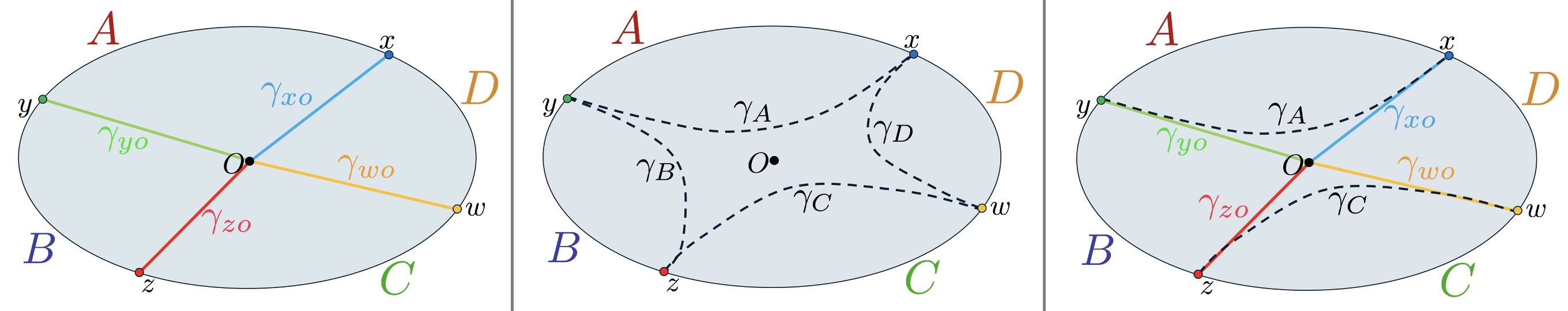
Figure 9: Left: For the case where holographic multi-entropy is given by the sum of the four surfaces, $\gamma_{xo}$, $\gamma_{yo}$, $\gamma_{zo}$ and $\gamma_{wo}$. Middle: RT surfaces $\gamma_{A}$, $\gamma_{B}$, $\gamma_{C}$, $\gamma_{D}$ for the entanglement entropy $S_{A}$, $S_{B}$, $S_{C}$, $S_{D}$. Right: (4) reduces to the summing over positive surfaces.

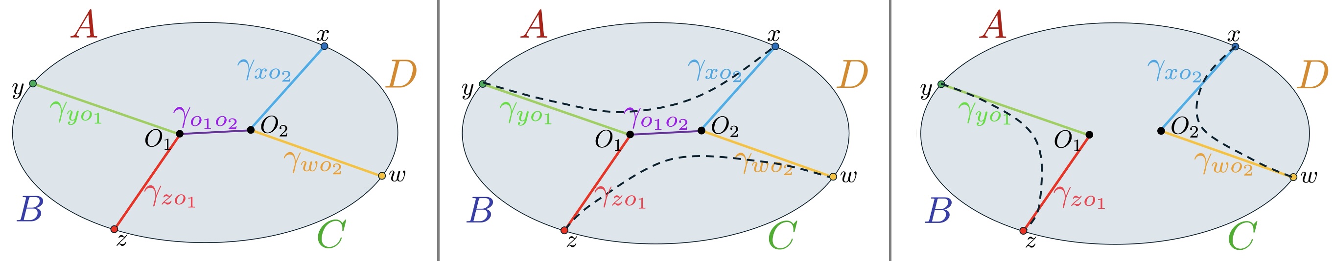
Figure 10: Left: For the case where holographic multi-entropy is given by the sum of the five surfaces, $\gamma_{xo_{2}}$, $\gamma_{yo_{1}}$, $\gamma_{zo_{1}}$, $\gamma_{wo_{2}}$ and $\gamma_{o_{1}o_{2}}$. Middle and Right: Subtracting the RT surfaces gives positive in both cases.

So far we have assumed that the boundary subregions $A_{1},A_{2},\dots,A_{\mathtt{q}}$ are connected subregions. It is straightforward to generalize these proofs to the cases where the boundary subregions are disconnected. However, for such cases, there is a possibility that in the bulk, holographic dual does not admit “intersection surfaces”, such as $O$ in Fig. 9 and $O_{1}$, $O_{2}$ in Fig. 10. For example, see figure 11 in Harper:2024ker . In such cases, there is a case that an inequality (64) can be saturated. For example, if the disconnected subregion $A$ is much larger than subregions $B$ and $C$ as shown in the right figure of Fig. 11, the holographic multi-entropy and the holographic entanglement entropy are given by

$$S^{(3)}(A:B:C)=S_{A}=\frac{1}{4G_{N}}\left(\gamma_{B}+\gamma_{C}\right),\;\;\;S_{B}=\frac{1}{4G_{N}}\gamma_{B},\;\;\;S_{C}=\frac{1}{4G_{N}}\gamma_{C}.$$ (65)

Thus, if there are “intersection surfaces” in the bulk for holographic dual of multi-entropy, inequality (64) holds, but if not, the inequality (64) can be saturated. Thus, we conclude

$$S^{(\mathtt{q})}(A_{1}:A_{2}:\cdots:A_{\mathtt{q}})-\frac{1}{2}\left(\sum_{k=1}^{\mathtt{q}}S^{(2)}(A_{k})\right)\geq 0.$$ (66)

The equality can hold only if there is no “intersection surfaces” in the bulk.

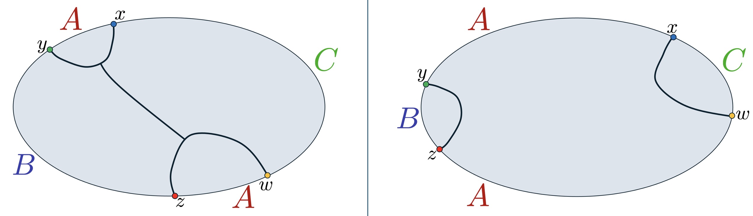
Figure 11: For the case where holographic multi-entropy is given by surfaces admitting “intersection surfaces” as the left figure, (66) is positive, but if it is not, as shown in the right figure, (66) is saturated.

This argument is parallel to the case of the holographic Markov gap Akers:2019gcv ; Hayden:2021gno . In holography, there are cases where the Markov gap becomes zero as well.

5 Generalization to $\mathtt{q}\geq 4$ cases

Similarly to $\mathtt{q}=3$, by taking appropriate linear combinations of multi-entropy, one can define genuine multi-entropy for the $\mathtt{q}\geq 4$ case as well. In fact, for the $\mathtt{q}=4$ case, we can define the following linear combination;

$$GM_{n}^{(4)}(A:B:C:D):=S_{n}^{(4)}(A:B:C:D)-\frac{1}{3}\Big{(}S_{n}^{(3)}(AB:C:D)+S_{n}^{(3)}(AC:B:D)$$

$$\qquad\qquad+S_{n}^{(3)}(AD:B:C)+S_{n}^{(3)}(BC:A:D)+S_{n}^{(3)}(BD:A:C)+S_{n}^{(3)}(CD:A:B)\Big{)}$$

$$\qquad+a\left(S_{n}^{(2)}(AB:CD)+S_{n}^{(2)}(AC:BD)+S_{n}^{(2)}(AD:BC)\right)$$

$$\qquad+b\left(S_{n}^{(2)}(ABC:D)+S_{n}^{(2)}(ABD:C)+S_{n}^{(2)}(ACD:B)+S_{n}^{(2)}(BCD:A)\right),$$ (67)

where $S_{n}^{(\mathtt{q})}$ is $\mathtt{q}$-partite Rényi multi-entropy, and $a$ and $b$ are parameters satisfying

$$a+b=\frac{1}{3}\,.$$ (68)

This can also be expressed in terms of the genuine tripartite multi-entropies such as $GM_{n}^{(3)}(AB:C:D)$ for three subsystems $AB$, $C$, $D$ defined in (23) as

$$GM_{n}^{(4)}(A:B:C:D):=S_{n}^{(4)}(A:B:C:D)-\frac{1}{3}\Big{(}GM_{n}^{(3)}(AB:C:D)+GM_{n}^{(3)}(AC:B:D)$$

$$\quad+GM_{n}^{(3)}(AD:B:C)+GM_{n}^{(3)}(BC:A:D)+GM_{n}^{(3)}(BD:A:C)+GM_{n}^{(3)}(CD:A:B)\Big{)}$$

$$\qquad+\tilde{a}\left(S_{n}^{(2)}(AB:CD)+S_{n}^{(2)}(AC:BD)+S_{n}^{(2)}(AD:BC)\right)$$

$$\qquad+\tilde{b}\left(S_{n}^{(2)}(ABC:D)+S_{n}^{(2)}(ABD:C)+S_{n}^{(2)}(ACD:B)+S_{n}^{(2)}(BCD:A)\right),$$ (69)

where

$$\tilde{a}+\tilde{b}=-\frac{1}{2}\,.$$ (70)

The claim is that this combination excludes the tripartite and bipartite entanglement and captures only the quadripartite entanglement only. This means, $GM_{n}^{(4)}(A:B:C:D)$ is zero for pure states with tripartite or bipartite entanglement such as

$$|\psi_{1}\rangle_{ABC}\otimes|\psi_{2}\rangle_{D},\;\;\;|\psi_{1}\rangle_{AB}\otimes|\psi_{2}\rangle_{CD}\,.$$ (71)

This can be seen as follows.

1. Consider a tripartite state, for example, $|\psi_{1}\rangle_{ABC}\otimes|\psi_{2}\rangle_{D}$. In this case, we do not need to contract the index of subsystem $D$, and the contraction of $n^{3}$ reduced density matrices for $S_{n}^{(4)}$ is factorized to $n$ product of the contraction of $n^{2}$ reduced density matrices due to the definition of the multi-entropy. Then, the following identities hold

   $$S_{n}^{(4)}(A:B:C:D)\qquad$$

   $$=S_{n}^{(3)}(AD:B:C) =S_{n}^{(3)}(BD:A:C)=S_{n}^{(3)}(CD:A:B),$$ (72)

   $$S_{n}^{(3)}(AB:C:D) =S_{n}^{(2)}(AB:CD)=S_{n}^{(2)}(ABD:C),$$ (73)

   $$S_{n}^{(3)}(AC:B:D) =S_{n}^{(2)}(AC:BD)=S_{n}^{(2)}(ACD:B),$$ (74)

   $$S_{n}^{(3)}(BC:A:D) =S_{n}^{(2)}(AD:BC)=S_{n}^{(2)}(BCD:A),$$ (75)

   $$S_{n}^{(2)}(ABC:D)=0.$$ (76)

   (A:) - (75) give

   $$S_{n}^{(4)}(A:B:C:D)\qquad\qquad\qquad\qquad\qquad\qquad\qquad\qquad\qquad\qquad$$

   $$\quad-\frac{1}{3}\left(S_{n}^{(3)}(AD:B:C)+S_{n}^{(3)}(BD:A:C)+S_{n}^{(3)}(CD:A:B)\right) =0,$$ (77)

   $$-\frac{1}{3}S_{n}^{(3)}(AB:C:D)+aS_{n}^{(2)}(AB:CD)+bS_{n}^{(2)}(ABD:C) =0,$$ (78)

   $$-\frac{1}{3}S_{n}^{(3)}(AC:B:D)+aS_{n}^{(2)}(AC:BD)+bS_{n}^{(2)}(ACD:B) =0,$$ (79)

   $$-\frac{1}{3}S_{n}^{(3)}(BC:A:D)+aS_{n}^{(2)}(AD:BC)+bS_{n}^{(2)}(BCD:A) =0.$$ (80)

   Combined these with (76), one can see that $GM_{n}^{(4)}(A:B:C:D)$ given by (5) vanishes.

2. Similarly, consider a bipartite state, for example, $|\psi_{1}\rangle_{AB}\otimes|\psi_{2}\rangle_{CD}$. Its contribution is decomposed into the sum of contributions of $|\psi_{1}\rangle_{AB}$ and $|\psi_{2}\rangle_{CD}$ due to the additive property (9). Thus, we consider only for a state $|\psi_{1}\rangle_{AB}$, where subsystems $C$ and $D$ are not entangled. Note that in this case, since genuine tripartite multi-entropies such as $GM_{n}^{(3)}(AC:B:D)$ do not contain any bipartite contributions, they vanish. In this case, the following identities hold

   $$S_{n}^{(4)}(A:B:C:D) =S_{n}^{(2)}(AC:BD)=S_{n}^{(2)}(AD:BC)$$

   $$=S_{n}^{(2)}(ACD:B)=S_{n}^{(2)}(BCD:A),$$ (81)

   $$S_{n}^{(2)}(AB:CD) =S_{n}^{(2)}(ABC:D)=S_{n}^{(2)}(ABD:C)=0\,.$$ (82)

   (B:) can be written as

   $$S_{n}^{(4)}(A:B:C:D) +\tilde{a}\left(S_{n}^{(2)}(AC:BD)+S_{n}^{(2)}(AD:BC)\right)$$

   $$+\tilde{b}\left(S_{n}^{(2)}(ACD:B)+S_{n}^{(2)}(BCD:A)\right)=0$$ (83)

   Using this with (82), one can see that $GM_{n}^{(4)}(A:B:C:D)$ given by (5) vanishes.

Thus, $GM_{n}^{(4)}(A:B:C:D)$ for tensor products of states like (71) are zero.

It is straightforward to generalize this construction for $\mathtt{q}\geq 5$. General prescription to construct the genuine $\mathtt{q}$-partite multi-entropy is followings. First, consider a general expression for the linear combination of $S_{n}^{(\mathtt{q})}$, $S_{n}^{(\mathtt{q}-1)}$, $\dots$, $S_{n}^{(2)}$ with symmetry in all the parties. Then, determine each coefficient of the linear combination so that the genuine $\mathtt{q}$-partite multi-entropy vanishes for states with $(\mathtt{q}-1)$-partite entanglement such as

$$|\psi\rangle=|\psi_{1}\rangle_{A_{1}A_{2}\dots A_{\mathtt{q}-1}}\otimes|\psi_{2}\rangle_{A_{\mathtt{q}}}.$$ (84)

We emphasize that the symmetric property (8) and the additive property (9) are crucial in this construction. It is interesting to investigate these higher $\mathtt{q}$ genuine multi-partite entanglement in more detail from both CFTs and also holography. It is quite interesting to investigate more details for higher $\mathtt{q}$ case.

6 Discussions and open questions

We end this paper with discussions on open questions:

1. We conjectured that $c_{W}>1$ in (17) by evaluating $S^{(3)}_{n}$ of the W-state for small $n$. Can we rigorously prove $c_{W}>1$? And, in three qubit systems, what state gives the maximum value of multi-entropy and genuine tripartite multi-entropy?

2. By assuming the holographic prescription of multi-entropy Gadde:2022cqi ; Gadde:2023zzj , we argued the inequality (66). Does this inequality hold even for non-holographic CFTs or general spin systems? Or does it only work in special cases, like the monogamy of holographic mutual information Hayden:2011ag ?

3. We assumed the holographic prescription of multi-entropy at $n\to 1$ Gadde:2022cqi ; Gadde:2023zzj . However, as demonstrated by Penington:2022dhr , in holographic CFTs, $S^{(3)}_{n}$ with $n\geq 3$ is not dual to the minimal triway cuts in the bulk, and thus the validity of holographic assumption at $n\to 1$ is unclear. At least, for pure states in RTN, the holographic assumption is plausible Penington:2022dhr , and our geometrical proof could be applied.

4. Our construction of the genuine $\mathtt{q}=4$ multi-entropy $GM_{n}^{(4)}(A:B:C:D)$ includes two free parameters $a,b$ or $\tilde{a},\tilde{b}$ as in eqs. (5) and (5). What is the role of these parameters? Can their values be determined by further requirements for genuine entanglement measures? For example, as a generalization of Fig. 4, we plot the black hole genuine multi-entropy curve of $GM^{(4)}(\text{R1}:\text{R2}:\text{R3}:\text{BH})$ in Fig. 12. One can see that $GM^{(4)}$ can be negative if $b$ is positive. Thus, if we impose that $GM^{(4)}$ is non-negative, $b$ should be non-positive.

5. Further detailed analysis on the genuine multi-entropy for $\mathtt{q}\geq 4$ is needed for both holography and generic quantum states. We would like to report it in the near future.

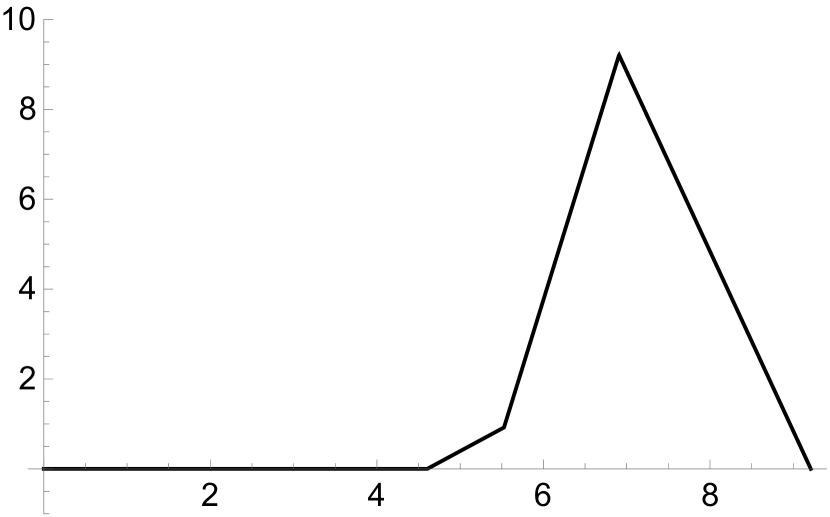
(a) $a=1/2,b=-1/6$

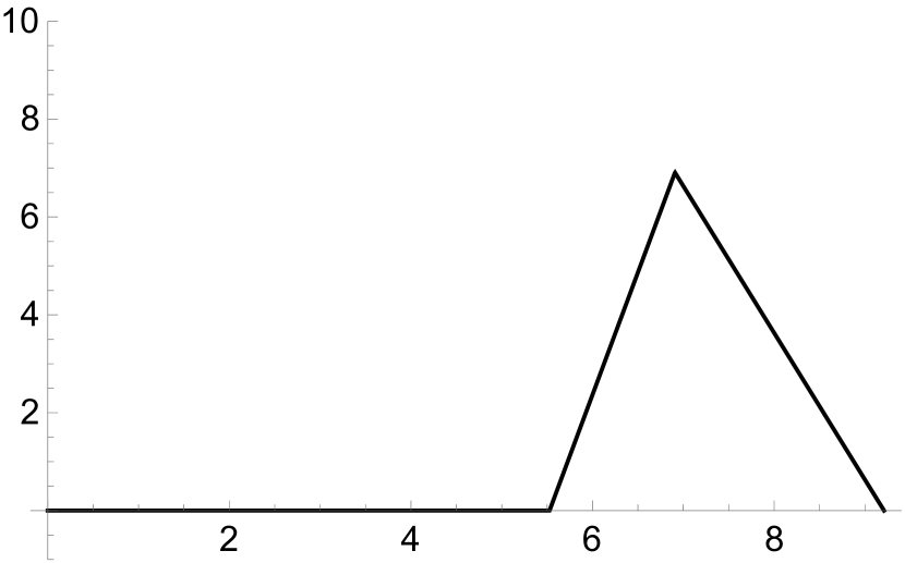
(b) $a=1/3,b=0$

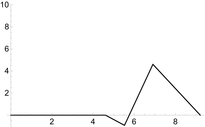
(c) $a=1/6,b=1/6$

Figure 12: Asymptotic behaviors of $GM^{(4)}(\text{R1}:\text{R2}:\text{R3}:\text{BH})$ for a Haar-random state with different values of $a$ and $b$, where $\dim\mathcal{H}_{\text{R1}}=\dim\mathcal{H}_{\text{R2}}=\dim\mathcal{H}_{\text{R3}}=d_{\text{R}}$, $\dim\mathcal{H}_{\text{BH}}=d_{\text{BH}}$, and we fix $d_{\rm Total}=d_{\rm BH}d_{\rm R}^{3}=10^{12}$. There are three time scales: (1) $d_{\text{R}}^{3}=d_{\text{BH}}$, (2) $d_{\text{R}}^{2}=d_{\text{BH}}$, and (3) $d_{\text{R}}=d_{\text{BH}}$.

Appendix A The maximum value of $S^{(3)}_{2}$ in W-class

Let us consider a pure state in W-class Dur:2000zz

$$|\psi_{W}\rangle=\sqrt{a}|001\rangle+\sqrt{b}|010\rangle+\sqrt{c}|100\rangle+\sqrt{d}|000\rangle,$$ (85)

where $a,b,c>0$ and $d=1-a-b-c\geq 0$. We want to find the value of $a,b,c,d$ to maximize $S^{(3)}_{2\;|\psi_{W}\rangle}$. To maximize $S^{(3)}_{2}$, replica partition function $Z_{2}^{(3)}$ should be minimum. By using $c=1-a-b-d$, one can express $Z_{2}^{(3)}$ of $|\psi_{W}\rangle$ as

$$Z_{2}^{(3)} =\left(2a^{2}+2a(b-1)+2b^{2}-2b+1\right)^{2}$$

$$+d(4(2a^{3}+2a^{2}(-1+b)+a(1-2b+2b^{2})+b(1-2b+2b^{2})))+(4a^{2}+4b^{2})d^{2}$$

$$=:f(a,b,d).$$ (86)

Our goal is to find the minimum value of $f(a,b,d)$.

First, we show that $f(a,b,d)$ is minimum at $d=0$ by analyzing

$$\frac{\partial f(a,b,d)}{\partial d}=-8a^{2}+8a^{3}+4b+8a^{2}b-8b^{2}+8b^{3}+4a(1-2b+2b^{2})+2(4a^{2}+4b^{2})d.$$ (87)

One can check that $\frac{\partial f(a,b,d)}{\partial d}\geq 0$ for $a,b>0$ and $d\geq 0$. Thus, $f(a,b,d)$ is minimum at $d=0$. Note that $\frac{\partial f(a,b,d)}{\partial d}=0$ at $a=b=0$. In this case, $f(0,0,d)=1$.

Next, we consider

$$f(a,b,0) =\left(2a^{2}+2a(b-1)+2b^{2}-2b+1\right)^{2},$$ (88)

$$\frac{\partial f(a,b,0)}{\partial b} =4(-1+a+2b)(1+2a^{2}+2a(-1+b)-2b+2b^{2}).$$ (89)

$\frac{\partial f(a,b,0)}{\partial b}$ becomes zero at $b=(1-a)/2$, where $a+(1-a)/2=(1+a)/2\leq 1$ for $0<a\leq 1$. There is no real solution of $b$ for $1+2a^{2}+2a(-1+b)-2b+2b^{2}=0$. We also obtain

$$\frac{\partial^{2}f(a,b,0)}{\partial b^{2}}|_{b=(1-a)/2}=4-8a+12a^{2}>0.$$ (90)

Thus, $f(a,b,0)$ is minimum at $b=(1-a)/2$.

Finally, we consider

$$f(a,(1-a)/2,0)=1/4(1-2a+3a^{2})^{2}.$$ (91)

Its minimum value is $1/9$ at $a=1/3$. Therefore, the minimum value of $Z_{2}^{(3)}$ is 1/9 at $a=1/3,b=(1-a)/2=1/3,c=1-a-b-d=1/3,d=0$. This state is W-state

$$|\text{W}\rangle=\frac{1}{\sqrt{3}}|001\rangle+\frac{1}{\sqrt{3}}|010\rangle+\frac{1}{\sqrt{3}}|100\rangle,$$ (92)

and the maximum value of $S^{(3)}_{2}$ in W-class is $S^{(3)}_{2\;{|\text{W}\rangle}}=\frac{1}{2}\log 9$.

Appendix B L-entropy and tripartite logarithmic negativity

A curve of L-entropy, which has been proposed by Basak:2024uwc , also has a similar behavior to genuine multi-entropy as in Figure 3. L-entropy $l_{ABC}$ in tri-partite systems is defined by

$$l_{ABC} :=[l_{AB}l_{BC}l_{CA}]^{1/3},$$ (93)

$$l_{AB} :=\text{Min}\{2S^{(2)}(A),2S^{(2)}(B)\}-S_{R}^{(1,1)}(A:B).$$ (94)

Assuming the holographic correspondence, a curve of L-entropy was computed by the bulk area in a three-boundary wormhole as shown in Figure 17 of Basak:2024uwc , which is similar to our black hole multi-entropy curve of genuine multi-entropy.

Note that $l_{AB}$ does not have the additive property (9), and thus $l_{ABC}$ of a triangle state $\ket{\Delta}_{ABC}=\ket{\psi_{1}}_{A_{R}B_{L}}\ket{\psi_{2}}_{B_{R}C_{L}}\ket{\psi_{3}}_{C_{R}A_{L}}$ can be nonzero. To see it, let us compute $l_{AB}$ of $\ket{\Delta}_{ABC}$. By using the additive property of $S^{(2)}$ and $S_{R}^{(1,1)}$, and

$$S_{R}^{(1,1)}(A:B)_{|\psi_{1}\rangle_{A_{R}B_{L}}} =2S^{(2)}(A)_{|\psi_{1}\rangle_{A_{R}B_{L}}}=2S^{(2)}(B)_{|\psi_{1}\rangle_{A_{R}B_{L}}},$$ (95)

$$S_{R}^{(1,1)}(A:B)_{|\psi_{2}\rangle_{B_{R}C_{L}}} =S_{R}^{(1,1)}(A:B)_{|\psi_{3}\rangle_{C_{R}A_{L}}}=0,$$ (96)

we obtain

$$\;\;\;\;\;l_{AB\;\ket{\Delta}}$$

$$=\text{Min}\{2S^{(2)}(A)_{|\psi_{1}\rangle_{A_{R}B_{L}}}+2S^{(2)}(A)_{|\psi_{3}\rangle_{C_{R}A_{L}}},2S^{(2)}(B)_{|\psi_{1}\rangle_{A_{R}B_{L}}}+2S^{(2)}(B)_{|\psi_{2}\rangle_{B_{R}C_{L}}}\}$$

$$\;\;\;\;\;-S_{R}^{(1,1)}(A:B)_{|\psi_{1}\rangle_{A_{R}B_{L}}}$$

$$=\text{Min}\{2S^{(2)}(A)_{|\psi_{3}\rangle_{C_{R}A_{L}}},2S^{(2)}(B)_{|\psi_{2}\rangle_{B_{R}C_{L}}}\},$$ (97)

which can be nonzero. Similarly,

$$l_{BC\;\ket{\Delta}}=\text{Min}\{2S^{(2)}(B)_{|\psi_{1}\rangle_{A_{R}B_{L}}},2S^{(2)}(C)_{|\psi_{3}\rangle_{C_{R}A_{L}}}\},$$ (98)

$$l_{CA\;\ket{\Delta}}=\text{Min}\{2S^{(2)}(C)_{|\psi_{2}\rangle_{B_{R}C_{L}}},2S^{(2)}(A)_{|\psi_{1}\rangle_{A_{R}B_{L}}}\},$$ (99)

can be also nonzero. Therefore, the tri-partite L-entropy $l_{ABC}$ (93) of the triangle state $\ket{\Delta}_{ABC}=\ket{\psi_{1}}_{A_{R}B_{L}}\ket{\psi_{2}}_{B_{R}C_{L}}\ket{\psi_{3}}_{C_{R}A_{L}}$ can be nonzero.

By using the negativity Vidal:2002zz , the tripartite negativity was defined by sabin2008 . In a similar way, we define tripartite logarithmic negativity $\mathcal{E}_{ABC}$ as follows.

$$\mathcal{E}_{ABC}:=[\mathcal{E}_{AB}\mathcal{E}_{BC}\mathcal{E}_{CA}]^{1/3},$$ (100)

where $\mathcal{E}_{AB}$ is the logarithmic negativity defined by

$$\mathcal{E}_{AB}:=\log\|\rho_{AB}^{T_{A}}\|_{1},$$ (101)

where $T_{A}$ means the partial transpose, and $\|\cdots\|_{1}$ is the trace norm. The asymptotic behavior of $\mathcal{E}_{AB}$ in a single random tensor model was derived by Bhosale:2012ldd ; Lu:2020jza ; Shapourian:2020mkc . By using their results, we plot a curve of $\mathcal{E}_{\text{R1R2BH}}$ with the total dimension $d_{\rm Total}=d_{\rm BH}d_{\rm R}^{2}=10^{12}$ in Figure 13, where the behavior is qualitatively similar to Figure 17 of Basak:2024uwc for L-entropy $l_{R1R2B}$.

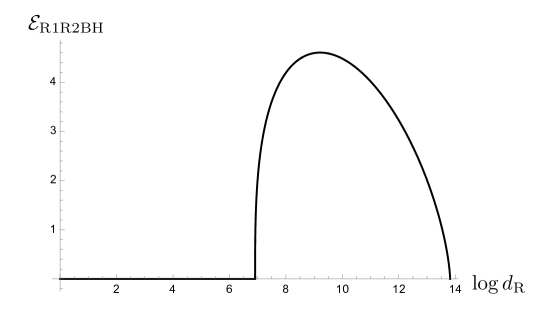
Figure 13: Asymptotic behavior of tripartite logarithmic negativity $\mathcal{E}_{\text{R1R2BH}}$.

References

- (1) C. Akers and P. Rath, Entanglement Wedge Cross Sections Require Tripartite Entanglement, JHEP 04 (2020) 208, [1911.07852].
- (2) P. Hayden, O. Parrikar and J. Sorce, The Markov gap for geometric reflected entropy, JHEP 10 (2021) 047, [2107.00009].
- (3) A. Gadde, V. Krishna and T. Sharma, New multipartite entanglement measure and its holographic dual, Phys. Rev. D 106 (2022) 126001, [2206.09723].
- (4) G. Penington, M. Walter and F. Witteveen, Fun with replicas: tripartitions in tensor networks and gravity, JHEP 05 (2023) 008, [2211.16045].
- (5) S. Ryu and T. Takayanagi, Holographic derivation of entanglement entropy from AdS/CFT, Phys. Rev. Lett. 96 (2006) 181602, [hep-th/0603001].
- (6) P. Hayden, S. Nezami, X.-L. Qi, N. Thomas, M. Walter and Z. Yang, Holographic duality from random tensor networks, JHEP 11 (2016) 009, [1601.01694].
- (7) M. Freedman and M. Headrick, Bit threads and holographic entanglement, Commun. Math. Phys. 352 (2017) 407–438, [1604.00354].
- (8) S. X. Cui, P. Hayden, T. He, M. Headrick, B. Stoica and M. Walter, Bit Threads and Holographic Monogamy, Commun. Math. Phys. 376 (2019) 609–648, [1808.05234].
- (9) W. Dur, G. Vidal and J. I. Cirac, Three qubits can be entangled in two inequivalent ways, Phys. Rev. A 62 (2000) 062314, [quant-ph/0005115].
- (10) S. Dutta and T. Faulkner, A canonical purification for the entanglement wedge cross-section, JHEP 03 (2021) 178, [1905.00577].
- (11) A. Gadde, V. Krishna and T. Sharma, Towards a classification of holographic multi-partite entanglement measures, JHEP 08 (2023) 202, [2304.06082].
- (12) X.-X. Ju, W.-B. Pan, Y.-W. Sun and Y. Zhao, Holographic multipartite entanglement from the upper bound of -partite information, 2411.07790.
- (13) X.-X. Ju, W.-B. Pan, Y.-W. Sun, Y.-T. Wang and Y. Zhao, More on the upper bound of holographic n-partite information, 2411.19207.
- (14) T. Mori and B. Yoshida, Does connected wedge imply distillable entanglement?, 2411.03426.
- (15) T. Mori and B. Yoshida, Tripartite Haar random state has no bipartite entanglement, 2502.04437.
- (16) J. Harper, T. Takayanagi and T. Tsuda, Multi-entropy at low Renyi index in 2d CFTs, SciPost Phys. 16 (2024) 125, [2401.04236].
- (17) Y. Zou, K. Siva, T. Soejima, R. S. K. Mong and M. P. Zaletel, Universal tripartite entanglement in one-dimensional many-body systems, Phys. Rev. Lett. 126 (2021) 120501, [2011.11864].
- (18) A. Gadde, S. Jain, V. Krishna, H. Kulkarni and T. Sharma, Monotonicity conjecture for multi-party entanglement. Part I, JHEP 02 (2024) 025, [2308.16247].
- (19) N. Iizuka, S. Lin and M. Nishida, Black Hole Multi-Entropy Curves, 2412.07549.
- (20) B. Liu, J. Zhang, S. Ohyama, Y. Kusuki and S. Ryu, Multi wavefunction overlap and multi entropy for topological ground states in (2+1) dimensions, 2410.08284.
- (21) M.-K. Yuan, M. Li and Y. Zhou, Reflected multi-entropy and its holographic dual, 2410.08546.
- (22) A. Gadde, J. Harper and V. Krishna, Multi-invariants and Bulk Replica Symmetry, 2411.00935.
- (23) J. K. Basak, V. Malvimat and J. Yoon, A New Genuine Multipartite Entanglement Measure: from Qubits to Multiboundary Wormholes, 2411.11961.
- (24) D. N. Page, Average entropy of a subsystem, Phys. Rev. Lett. 71 (1993) 1291–1294, [gr-qc/9305007].
- (25) D. N. Page, Information in black hole radiation, Phys. Rev. Lett. 71 (1993) 3743–3746, [hep-th/9306083].
- (26) C. Akers, T. Faulkner, S. Lin and P. Rath, Reflected entropy in random tensor networks, JHEP 05 (2022) 162, [2112.09122].
- (27) R. Sohal and S. Ryu, Entanglement in tripartitions of topological orders: A diagrammatic approach, Phys. Rev. B 108 (2023) 045104, [2301.07763].
- (28) C. Berthiere and G. Parez, Reflected entropy and computable cross-norm negativity: Free theories and symmetry resolution, Phys. Rev. D 108 (2023) 054508, [2307.11009].
- (29) P. Hayden, M. Headrick and A. Maloney, Holographic Mutual Information is Monogamous, Phys. Rev. D 87 (2013) 046003, [1107.2940].
- (30) G. Vidal and R. F. Werner, Computable measure of entanglement, Phys. Rev. A 65 (2002) 032314, [quant-ph/0102117].
- (31) C. Sabín and G. García-Alcaine, A classification of entanglement in three-qubit systems, Eur. Phys. J. D 48 (2008) 435–442, [0707.1780].
- (32) U. T. Bhosale, S. Tomsovic and A. Lakshminarayan, Entanglement between two subsystems, the Wigner semicircle and extreme-value statistics, Phys. Rev. A 85 (2012) 062331.
- (33) T.-C. Lu and T. Grover, Entanglement transitions as a probe of quasiparticles and quantum thermalization, Phys. Rev. B 102 (2020) 235110, [2008.11727].
- (34) H. Shapourian, S. Liu, J. Kudler-Flam and A. Vishwanath, Entanglement Negativity Spectrum of Random Mixed States: A Diagrammatic Approach, PRXQuantum 2 (2021) 030347, [2011.01277].