Causal Additive Models with Unobserved Causal Paths and Backdoor Paths

Abstract

Causal additive models have been employed as tractable yet expressive frameworks for causal discovery involving hidden variables. State-of-the-art methodologies suggest that determining the causal relationship between a pair of variables is infeasible in the presence of an unobserved backdoor or an unobserved causal path. Contrary to this assumption, we theoretically show that resolving the causal direction is feasible in certain scenarios by incorporating two novel components into the theory. The first component introduces a novel characterization of regression sets within independence between regression residuals. The second component leverages conditional independence among the observed variables. We also provide a search algorithm that integrates these innovations and demonstrate its competitive performance against existing methods.

1 Introduction

Causal Additive Models (CAMs) [Bühlmann et al., 2014b] are nonlinear causal models in which the causal effects and the error terms are additive. Due to their tractability, they have been studied considerably and have many practical applications in machine learning [Budhathoki et al., 2022, Yokoyama et al., 2025].

When there are hidden variables, the problem of causal discovery in CAM, i.e., identification of the causal graph, remains underexplored, limiting its practical adoption where hidden variables are almost always present. Although causal discovery with hidden variables can be treated in full generality by the framework of Fast Causal Inference (FCI) [Spirtes et al., 2000], it is natural to expect that we can do better than FCI in certain aspects by exploiting specific properties of CAMs.

Maeda and Shimizu [2021] identify cases in which the parent-child relationship in CAMs can be determined in the presence of unobserved variables by analyzing independencies and dependencies between certain regression residuals. This is significant and relies on specific properties of CAMs, as parent-child relationships are unidentifiable in the FCI framework.

Although Maeda and Shimizu [2021] allow for hidden variables, their results require that no unobserved backdoor or causal paths exist. If such paths are present, they consider the parent-child relationship unidentifiable.

Schultheiss and Bühlmann [2024] provide sufficient conditions for identifying the causal effect of an observed variable $X_{i}$ on another observed variable $X_{j}$ in nonlinear additive noise models with unobserved variables. While they do not discuss causal search as an application of their theory, it can formally be used to identify causal directions in CAMs: if the causal effect is nonzero, $X_{i}$ can be identified as an ancestor of $X_{j}$.

Focusing on CAMs with unobserved variables, we show that a) the parent-child relationship can be identified in certain cases even in the presence of an unobserved backdoor or causal path, which is an improvement over Maeda and Shimizu [2021], and b) some causal directions beyond those identified by Schultheiss and Bühlmann [2024] can be determined. A high-level summary of our main contributions is as follows.

• By characterizing the regression sets used in determining independence, we show that the causal direction between a pair of variables can sometimes be identified using independence between the residuals, even when there are unobserved backdoor paths. We give an example, in Remark 1, of a causal direction that can be identified by this approach but cannot be identified by the theory of Schultheiss and Bühlmann [2024].

• We introduce a novel identification strategy that combines conditional independence between the original variables with independence between regression residuals to identify causal directions or parent-child relationships in certain pairs of observed variables, even in the presence of unobserved backdoor and causal paths. In Remark 2, we provide an example of a causal direction identifiable by this new approach but not by the theory of Schultheiss and Bühlmann [2024].

• We introduce CAM-UV-X, an extension of the CAM-UV algorithm of Maeda and Shimizu [2021]. Our algorithm incorporates the above innovations to identify parent-child relationships and causal directions in the presence of unobserved backdoor and causal paths. Additionally, it addresses a previously overlooked limitation of the CAM-UV algorithm in identifying causal relationships when all backdoor and causal paths are observable.

The paper is organized as follows. We review the background in Section 2. New identifiability results are presented in Section 3. Our proposed search method based on these theoretical results is described in Section 4. Related works are discussed in Section 5. Numerical experiments are provided in Section 6. Conclusions are given in Section 7.

2 Preliminaries

2.1 The causal Model

We assume the following causal additive model with unobserved variables as in Maeda and Shimizu [2021]. Let $X=\{x_{i}\}$ and $U=\{u_{i}\}$ be the sets of observable and unobservable variables, respectively. $G=(V,E)$ is the DAG with the vertex set $V=\{v_{i}\}=X\cup U$ and the edge set $E=\{(i,j)\mid v_{i}\in V,v_{j}\in V\}$. The data generation model is

$$v_{i}=\sum_{j\in P_{i}}f_{j}^{(i)}(x_{j})+\sum_{k\in Q_{i}}f_{k}^{(i)}(u_{k})+n_{i},$$ (1)

where $P_{i}=\{j\mid(i,j)\in V\land x_{j}\in X\}$ is the set of observable direct causes of $v_{i}$, $Q_{i}=\{k\mid(i,k)\in V\land u_{k}\in U\}$ is the set of unobservable direct causes of $v_{i}$, $f_{j}^{(i)}$ is a non-linear function, and $n_{i}$ is the external noise at $v_{i}$. The functions and the external noises are assumed to satisfy Assumption 1 of Maeda and Shimizu [2021] (see Appendix A).

2.2 Unobserved backdoor paths and unobserved causal paths

Unobserved backdoor paths (UBPs) and unobserved causal paths (UCPs) play central roles in the theory of causal additive models with unobserved variables [Maeda and Shimizu, 2021].

Definition 2.1 (Unobserved Causal Path).

A path in $G$ is called an unobserved causal path between $x_{i}$ and $x_{j}$ iff it is of the form $x_{i}\rightarrow\cdots\rightarrow u_{k}\rightarrow x_{j}$.

Definition 2.2 (Unobserved Backdoor Path).

A path in $G$ is called an unobserved backdoor path between $x_{i}$ and $x_{j}$ iff it is of the form $x_{i}\leftarrow u_{k}\leftarrow\cdots v_{i}\rightarrow\cdots\rightarrow u_{l}\rightarrow x_{j}$.

Figs. 1a and b illustrate UCPs and UBPs, respectively.

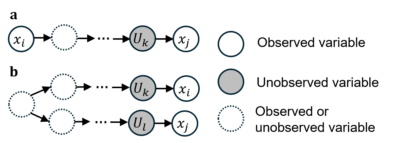
Figure 1: Illustrations of unobserved backdoor paths and unobserved causal paths.

When a UBP or a UCP exists between $x_{i}$ and $x_{j}$, the confounder effect of the UBP or the causal effect of the UCP cannot be fully eliminated by regressions on any set of observed variables [Maeda and Shimizu, 2021]. Consequently, the presence or absence of an edge between $x_{i}$ and $x_{j}$ and the direction of causality are obscured. This intuition is formalized in the next section.

2.3 Visible and invisible pairs

The following concepts of visible parents, visible non-edge, and invisible pairs are fundamental to both the CAM-UV algorithm and our proposed CAM-UV-X. The lemmas are introduced and proved in Maeda and Shimizu [2021]. In these lemmas, $\mathcal{G}$ is a subclass of the generalized additive models (GAMs) [Hastie and Tibshirani, 1986] that additionally satisfies Assumption 2 of Maeda and Shimizu [2021] (see Appendix A). For a function $G_{i}\in\mathcal{G}$, since $G_{i}$ belongs to GAMs, $G_{i}(N)=\sum_{x_{m}\in N}g_{i,m}(x_{m})$ where each $g_{i,m}(x_{m})$ is a nonlinear function of $x_{m}$.

Lemma 2.1 (visible parent).

If and only if Eqs. (2) and (3) are satisfied, $x_{j}$ is a parent of $x_{i}$, and there is no UBP or UCP between $x_{j}$ and $x_{i}$. We call $x_{j}$ a visible parent of $x_{i}$.

$$\forall G_{1},G_{2}\in\mathcal{G},M\subseteq X\setminus\{x_{i},x_{j}\},N\subseteq X\setminus\{x_{j}\}:$$

$$x_{i}-G_{1}(M)\mathrel{\,\not\!\mathrel{\perp\mspace{-9.0mu}\perp}}x_{j}-G_{2}(N),$$ (2)

$$\exists G_{1},G_{2}\in\mathcal{G},M\subseteq X\setminus\{x_{i}\},N\subseteq X\setminus\{x_{i},x_{j}\}:$$

$$x_{i}-G_{1}(M)\mathrel{\perp\mspace{-9.0mu}\perp}x_{j}-G_{2}(N).$$ (3)

Lemma 2.2 (visible non-edge).

If and only if Eq. (4) is satisfied, there is no direct edge between $x_{j}$ and $x_{i}$, and there is no UBP or UCP between $x_{j}$ and $x_{i}$. $(x_{i},x_{j})$ is called a visible non-edge.

$$\exists G_{1},G_{2}\in\mathcal{G},M\subseteq X\setminus\{x_{i},x_{j}\},N\subseteq X\setminus\{x_{i},x_{j}\}:$$

$$x_{i}-G_{1}(M)\mathrel{\perp\mspace{-9.0mu}\perp}x_{j}-G_{2}(N).$$ (4)

Lemma 2.3 (invisible pairs).

If and only if Eq. (5) is satisfied, there is a UBP/UCP between $x_{j}$ and $x_{i}$. $(x_{i},x_{j})$ is called an invisible pair.

$$\forall M\subseteq X\setminus\{x_{i}\},N\subseteq X\setminus\{x_{j}\},\forall G_{i},G_{j}\in\mathcal{G}:$$

$$x_{i}-G_{i}(M)\mathrel{\,\not\!\mathrel{\perp\mspace{-9.0mu}\perp}}x_{j}-G_{j}(N).$$ (5)

Visible pairs are identifiable from the observed data, by checking Eqs. (2) and (3) for the case of a visible edge, and checking Eq. (4) for the case of a visible non-edge. Similarly, Eq. (5) can certify that a pair is invisible from the observed data. However, Eq. (5) cannot identify the causal directions in invisible pairs.

The CAM-UV algorithm [Maeda and Shimizu, 2021] is designed to detect visible edges and non-edges while marking invisible pairs as such. However, it does not identify causal directions in invisible pairs.

3 Identifiability in invisible pairs

We present new results that identify parent-child relationships and causal directions in invisible pairs. All omitted proofs can be found in Appendix B.

3.1 Identifiability by independence between regression residuals

In this section, identifiability improvements come from characterizing the content of the regression sets $M$ and $N$ in Lemmas 2.1 and 2.2.

We provide Lemma 3.1 to characterize the regression sets in Eq. (3). For a visible edge $(x_{i},x_{j})$, the lemma tells us cases where one can infer that some variable $x_{k}$ in $M$ or $N$ must be a parent of $x_{i}$ or $x_{j}$.

Lemma 3.1.

Consider distinct $x_{i}$, $x_{j}$, and $x_{k_{1}},\cdots,x_{k_{n}}$. Let $K=\{x_{k_{1}},\cdots,x_{k_{n}}\}$. If Eqs. (6), (7), and (8) are satisfied, then

1. $x_{j}$ is a visible parent of $x_{i}$, and

2. Each $x_{k_{q}}$ is a parent of $x_{j}$ or a parent of $x_{i}$. Since $x_{j}$ is a parent of $x_{i}$, each $x_{k_{q}}$ is thus an ancestor of $x_{i}$.

$$\text{For }q=1,\cdots,n:\forall M\subseteq X\setminus\{x_{i},x_{k_{q}}\},$$

$$N\subseteq X\setminus\{x_{j},x_{k_{q}}\},\forall G_{i}^{1},G_{j}^{1}\in\mathcal{G}:$$

$$x_{i}-G_{i}^{1}(M)\mathrel{\,\not\!\mathrel{\perp\mspace{-9.0mu}\perp}}x_{j}-G_{j}^{1}(N),$$ (6)

$$\forall M\subseteq X\setminus\{x_{i},x_{j}\},N\subseteq X\setminus\{x_{j}\},\forall G_{i}^{1},G_{j}^{1}\in\mathcal{G}:$$

$$x_{i}-G_{i}^{1}(M)\mathrel{\,\not\!\mathrel{\perp\mspace{-9.0mu}\perp}}x_{j}-G_{j}^{1}(N),$$ (7)

$$\exists Q_{1},Q_{2}\subseteq K:Q_{1}\cup Q_{2}=K,Q_{1}\cap Q_{2}=\varnothing:$$

$$\exists G_{i}^{2},G_{j}^{2}\in\mathcal{G},M,N\subseteq X\setminus\{x_{i},x_{j}\}\setminus K:$$

$$x_{i}-G_{i}^{2}\left(M\cup\{x_{j}\}\cup Q_{1}\right)\mathrel{\perp\mspace{-9.0mu}\perp}x_{j}-G_{j}^{2}(N\cup Q_{2})$$ (8)

The intuition is that changes in independence status between regression residuals when a variable in $K$ is included/excluded from $M$ or $N$ allow inference of causal relationships between that variable and $x_{i}$, $x_{j}$, even when such relationships are invisible.

Example 1. In Fig. 2a, let $x_{i}=x_{2}$, $x_{j}=x_{1}$, $K=\{x_{3}\}$, $Q_{1}=\{x_{3}\}$, and $Q_{2}=\varnothing$. The variable $x_{3}$ is needed to block the backdoor path $x_{1}\leftarrow U_{1}\rightarrow x_{3}\rightarrow x_{2}$ between $x_{1}$ and $x_{2}$. Therefore, $x_{2}-G_{2}(M)$ and $x_{1}-G_{1}(N)$ cannot be independent for any $M\subseteq X\setminus\{x_{2},x_{3}\}$ and $N\subseteq X\setminus\{x_{1},x_{3}\}$, i.e., Eq. (6) is satisfied. When $x_{3}$ is included to the regression set, all backdoor/causal paths are blocked, thus we have $\exists G_{1},G_{2}:x_{2}-G_{2}(x_{1},x_{3})\mathrel{\perp\mspace{-9.0mu}\perp}x_{1}$, i.e., Eq. (8) is satisfied. Furthermore, $x_{2}-G_{2}(M)$ and $x_{1}-G_{1}(N)$ cannot be independent for any $M\subseteq\{x_{1},x_{2}\}$, $N\subseteq X\setminus\{x_{1}\}$, i.e., Eq. (7) is satisfied. By Lemma 3.1, the edge $x_{1}\rightarrow x_{2}$ is identified and $x_{3}$ can be identified to be an ancestor of $x_{2}$, even when $(x_{3},x_{2})$ is invisible.

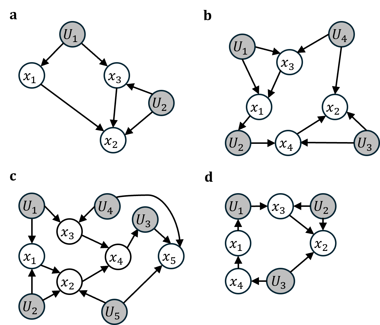
Figure 2: Examples of identifying causal relationships in the presence of UBPs/UCPs.

Remark 1.

In Fig. 2a, since no set of observed variables can d-separate $x_{3}$ and $U_{2}$, the condition (A1) of Schultheiss and Bühlmann [2024] cannot be satisfied. Therefore, their theory cannot identify the causal effect from $x_{3}$ to $x_{2}$, and thus cannot identify that $x_{3}$ is an ancestor of $x_{2}$.

Similarly, we have the following lemma to characterize the regression sets in Eq. (4) in the case of a visible non-edge:

Lemma 3.2.

Consider distinct $x_{i}$, $x_{j}$, and $x_{k_{1}},\cdots,x_{k_{n}}$. Let $K=\{x_{k_{1}},\cdots,x_{k_{n}}\}$. If Eqs. (6) and (9) are satisfied, then

1. $(x_{j},x_{i})$ is a visible non-edge, and

2. Each $x_{k_{q}}$ is either a parent of $x_{i}$ or a parent of $x_{j}$.

$$\exists Q_{1},Q_{2}\subseteq K:Q_{1}\cup Q_{2}=K,Q_{1}\cap Q_{2}=\varnothing:$$

$$\exists G_{i}^{2},G_{j}^{2}\in\mathcal{G},M,N\subseteq X\setminus\{x_{i},x_{j}\}\setminus K:$$

$$x_{i}-G_{i}^{2}\left(M\cup Q_{1}\right)\mathrel{\perp\mspace{-9.0mu}\perp}x_{j}-G_{j}^{2}(N\cup Q_{2}).$$ (9)

Example 2. In Fig. 2b, let $x_{i}=x_{1}$, $x_{j}=x_{2}$, $K=\{x_{3},x_{4}\}$, $Q_{1}=\{x_{3}\}$, and $Q_{2}=\{x_{4}\}$. The variable $x_{4}$ is needed to block the backdoor path $x_{1}\leftarrow U_{2}\rightarrow x_{4}\rightarrow x_{2}$ between $x_{1}$ and $x_{2}$. Similarly, the variable $x_{3}$ is needed to block the backdoor path $x_{1}\leftarrow x_{3}\leftarrow U_{4}\rightarrow x_{2}$. Therefore, $x_{2}-G_{2}(M)$ and $x_{1}-G_{1}(N)$ cannot be independent for any $M,N$ that do not contain $x_{3}$ or $x_{4}$, i.e., Eq. (6) is satisfied. When $x_{3}$ and $x_{4}$ are included to the regression set, all backdoor/causal paths are blocked, thus we have $\exists G_{1},G_{2}:x_{2}-G_{2}(x_{4})\mathrel{\perp\mspace{-9.0mu}\perp}x_{1}-G_{1}(x_{3})$, i.e., Eq. (9) is satisfied. By Lemma 3.1, the non-edge $(x_{1},x_{2})$ is identified, $x_{3}$ is identified as a parent of $x_{1}$ or $x_{2}$, and $x_{4}$ is also identified as a parent of $x_{1}$ or $x_{2}$.

3.2 Identifiability by Conditional Independence

In this section, identifiability improvements come from a novel approach of combining independence between regression residuals and conditional independence between the original variables.

We introduce the following key lemma.

Lemma 3.3.

If $x_{k}$ is an ancestor of $x_{i}$ and $x_{k}\mathrel{\perp\mspace{-9.0mu}\perp}x_{j}\mid x_{i}$, then

1. There is no backdoor path between $x_{i}$ and $x_{j}$, and

2. $x_{j}$ is not an ancestor of $x_{i}$.

Although Lemma 3.3 can be used alone to identify that $x_{j}$ is not an ancestor of $x_{i}$, combining it with independence conditions between regression residuals can identify the parent-child relation or the causal direction in certain invisible pairs as in the following corollaries.

Corollary 3.3.1.

If Eq. (5) is satisfied, and $x_{k}$ is an ancestor of $x_{i}$ and $x_{k}\mathrel{\perp\mspace{-9.0mu}\perp}x_{j}\mid x_{i}$, then $x_{i}$ is an ancestor of $x_{j}$.

Proof.

Eq. (5) implies that a UBP/UCP must exist between $x_{i}$ and $x_{j}$, due to Lemma 2.3. Lemma 3.3 rules out the possibilities of any UBP and the causal direction from $x_{j}$ to $x_{i}$. Therefore, the only possible scenario is that there is a UCP from $x_{i}$ to $x_{j}$, which means $x_{i}$ is an ancestor of $x_{j}$. ∎

Corollary 3.3.2.

Suppose that $x_{k}$ is a parent of $x_{i}$ or a parent of $x_{j}$ (e.g., by Lemma 3.1 or Lemma 3.2). Furthermore, for a fourth variable $x_{u}$, if $x_{u}$ is an ancestor of $x_{i}$ and $x_{u}\mathrel{\perp\mspace{-9.0mu}\perp}x_{k}\mid x_{i}$, then $x_{k}$ is a parent of $x_{j}$.

Proof.

Lemma 3.3 implies that $x_{k}$ is not an ancestor, and thus not a parent, of $x_{i}$. Therefore, the only possibility is that $x_{k}$ is a parent of $x_{j}$. ∎

Example 3. In Fig. 2c, consider the invisible pair $(x_{4},x_{5})$. Since this pair is not on any backdoor path or causal path of any visible pair, Lemmas 3.1 and 3.2 cannot identify the causal direction in this pair. From the visible pairs $(x_{2},x_{4})$ and $(x_{3},x_{4})$, $x_{2}$ and $x_{3}$ are identified to be parents of $x_{4}$ by Lemma 2.1. From the visible non-edge $(x_{2},x_{3})$, $x_{1}$ is identified to be a parent of $x_{2}$ or a parent of $x_{3}$ by applying Lemma 3.2 with $K=\{x_{1}\}$. Thus, $x_{1}$ is identified to be an ancestor of $x_{4}$. The ancestors of $x_{4}$ are $x_{2}$, $x_{3}$, and $x_{1}$. Since $x_{2}\mathrel{\,\not\!\mathrel{\perp\mspace{-9.0mu}\perp}}x_{5}\mid x_{4}$ and $x_{3}\mathrel{\,\not\!\mathrel{\perp\mspace{-9.0mu}\perp}}x_{5}\mid x_{4}$ due to the unobserved $U_{4}$ and $U_{5}$, Corollary 3.3.1 cannot be applied with $x_{k}=x_{2}$ or $x_{k}=x_{3}$. Nevertheless, we have $x_{1}\mathrel{\perp\mspace{-9.0mu}\perp}x_{5}\mid x_{4}$. After checking Eq. (5) for $x_{i}=x_{4}$ and $x_{j}=x_{5}$, we can identify $x_{4}$ as an ancestor of $x_{5}$ by applying Corollary 3.3.1 with $x_{k}=x_{1}$.

Remark 2.

In Fig. 2c, since no set of observed variables can d-separate $x_{4}$ and $U_{3}$, the condition (A1) of Schultheiss and Bühlmann [2024] cannot be satisfied. Thus, their theory cannot identify that $x_{4}$ is an ancestor of $x_{5}$.

Example 4. Consider the invisible pair $(x_{2},x_{3})$ in Fig 2d. Note that Corollary 3.3.1 cannot identify the causal direction in this pair. Applying Lemma 3.2 to the visible non-edge $(x_{1},x_{2})$ with $K=\{x_{3}\}$, one can identify that $x_{3}$ is a parent of $x_{1}$ or a parent of $x_{2}$. The edge $x_{4}\rightarrow x_{1}$ is visible and thus can be identified. One can check that $x_{4}\mathrel{\perp\mspace{-9.0mu}\perp}x_{3}\mid x_{1}$. Applying Corollary 3.3.2 with $x_{k}=x_{3}$, $x_{i}=x_{1}$, $x_{j}=x_{2}$, and $x_{u}=x_{4}$ identifies $x_{3}$ as a parent of $x_{2}$.

Remark 3.

Identifying the causal directions between $(x_{3},x_{2})$ in Fig. 2a, $(x_{4},x_{5})$ in Fig. 2c, and $(x_{3},x_{2})$ in Fig. 2d, as well as the non-edge $(x_{1},x_{2})$ in Fig. 2b, relies on independence conditions between regression residuals specific to CAMs. General methods based solely on Markov equivalence classes of conditional independence, such as FCI, cannot make such identifications.

4 Search methods

In Section 4.1, we highlight previously overlooked limitations of the CAM-UV algorithm, which makes it erroneously identify certain visible pairs as invisible. We provide our method in Section 4.2.

4.1 Limitations of the CAM-UV algorithm

The CAM-UV algorithm is not complete in identifying visible edges/non-edges, and is not sound in identifying invisible pairs. Soundness and completeness are two concepts often used in evaluations of a causal discovery algorithm [Spirtes et al., 2000]. The concepts can be adapted to our context as follows. Recall that $E$ is the true edge set and $G$ is the true causal graph. Let $A$ denote the adjacency matrix estimated by an algorithm. An algorithm is complete for identifying visible edges iff $(i,j)\in E$ and $(i,j)$ is visible in $G$ implies $A(i,j)=1$ in the algorithm output. An algorithm is sound for identifying visible edges iff $A(i,j)=1$ implies $(i,j)\in E$ and $(i,j)$ is visible in $G$. Soundness and completeness can be defined similarly for visible non-edges and invisible pairs.

Fig. 2a can be used to demonstrate that CAM-UV is not complete in identifying visible edges and not sound in identifying invisible pairs. The edge $x_{1}\rightarrow x_{2}$ is visible, i.e., identifiable from observed data using Lemma 2.1. However, $x_{3}$ is an invisible parent of $x_{2}$ due to the unobserved $U_{2}$. In such cases, the CAM-UV algorithm in principle will erroneously mark the visible edge as invisible. See Appendix C for a proof obtained by executing CAM-UV step by step in this example.

Fig. 2b can be used to demonstrate that CAM-UV is also not complete in identifying visible non-edges. The non-edge $(x_{1},x_{2})$ is visible, i.e, identifiable from observed data by Lemma 2.2. However, to block all backdoor and causal paths between $x_{1}$ and $x_{2}$, one must add $x_{3}$ and $x_{4}$ to the regression sets in Eq. (4). Furthermore, the pairs $(x_{1},x_{3})$, $(x_{1},x_{4})$, $(x_{2},x_{3})$, and $(x_{2},x_{4})$ are all invisible. In this case, CAM-UV will erroneously mark the visible non-edge as invisible. See Appendix C for a step-by-step execution of CAM-UV in this example.

4.2 Proposed search method

Our proposed method, described in Algorithm 1, addresses the limitations of the CAM-UV algorithm by improving the identification of visible pairs. Additionally, it leverages Lemmas 3.1 and 3.2, as well as Corollaries 3.3.1 and 3.3.2, to infer parentships or causal directions in invisible pairs. The output of CAM-UV-X is $A$, $M_{1},\ldots,M_{p}$, $H_{1},\ldots,H_{p}$, and $C_{1},\ldots,C_{p}$. $A$ is the adjacency matrix over the observed variables. $A(i,j)=1$ if $x_{j}$ is inferred to be a parent of $x_{i}$, $0$ if there is no directed edge from $x_{j}$ to $x_{i}$, and NaN (Not a Number) if $(x_{i},x_{j})$ is inferred to be invisible. $M_{i}$ is the set of ancestors of $x_{i}$ identified by Lemma 3.1 and Corollary 3.3.1. $H_{i}$ is the set of nodes guaranteed to be not an ancestor of $x_{i}$, identified by, for example, Lemma 3.3. $C_{k}$ contains unordered pairs $[i,j]$ such that $x_{k}$ is a parent of $x_{i}$ or $x_{k}$ is a parent of $x_{j}$.

Algorithm 1 CAM-UV-X

Data: $n\times p$ data matrix $X$ for $p$ observed variables, maximum number of parents $d$, significant level $\alpha$

Result: $A$, $\{M_{1},\ldots,M_{p}\}$, $\{H_{1},\ldots,H_{p}\}$, $\{C_{1},\ldots,C_{p}\}$

$A\leftarrow$ CAM-UV($X,d,\alpha$)

Initialize $M_{i}\leftarrow\varnothing$, $H_{i}\leftarrow\varnothing$, $C_{i}\leftarrow\varnothing$ for $i=1,\ldots,p$

$noChange\leftarrow False$

while $noChange$ == False do

2    $noChange\leftarrow True$   Find the set $S=\{(i,j)\mid A(i,j)=A(j,i)=\text{NaN}\}$ for each $(i,j)\in S$ do

3       $noChange\leftarrow\texttt{checkVisible}(i,j)$

4    end for

5   Find the set $S=\{(i,j)\mid A(i,j)=A(j,i)=\text{NaN}\}$ for each $(i,j)\in S$ do

6       $noChange\leftarrow\texttt{checkCI}(i,j)$

7    end for

8   $noChange\leftarrow\texttt{checkParentInvi}()$

9 end while

In line 1, CAM-UV is executed to obtain an initial estimation of $A$. The Boolean variable $noChange$ indicates whether a modification has occurred in $A$ or in any $M_{1},\ldots,M_{p}$, $H_{1},\ldots,H_{p}$, $C_{1},\ldots,C_{p}$. CAM-UV-X executes the loop in line 4 until no further modification is detected.

The procedure checkVisible, described in Algorithm 2, tests whether each NaN element in the current matrix $A$ can be converted to $1$, that is, a visible edge, by Lemma 3.1 (lines 6-15), or to $0$, i.e., a visible non-edge, by Lemma 3.2 (lines 17-28).

Algorithm 2 checkVisible

Input: indices $i$ and $j$

Output: Boolean variable $noChange$

$P_{i}\leftarrow\{v\mid A(i,v)=1\}$; $P_{j}\leftarrow\{v\mid A(j,v)=1\}$

$Q\leftarrow\{k\mid A(j,k)=\text{NaN}\text{ and }A(i,k)=\text{NaN}\}$

for size in $1,\ldots,|Q|$ do

2    for each $K\subseteq Q,|K|==size$ do

3       for each $(Q_{1},Q_{2})$ such that $Q_{1}\cup Q_{2}=K$ and $Q_{1}\cap Q_{2}=\varnothing$ do

4          $e\leftarrow\widehat{\text{p-HSIC}}\big{(}x_{i}-G_{1}(P_{i}\cup\{x_{j}\}\cup Q_{1}\setminus\{x_{i}\}),$ $x_{j}-G_{2}(P_{j}\cup Q_{2}\setminus\{x_{i}\}\setminus\{x_{j}\})\big{)}$ if $e>\alpha\ \land$ checkTrueEdge(i,j) then

5             $noChange\leftarrow False$ $A(i,j)\leftarrow 1$; $A(j,i)\leftarrow 0$ for $k\in K$ do

6                if checkOnPath(i,j,k) then

7                   $C_{k}\leftarrow C_{k}\cup\{[i,j]\}$; $M_{i}\leftarrow M_{i}\cup\{x_{k}\}$; $H_{k}\leftarrow H_{k}\cup\{x_{i}\}$; $A(k,i)\leftarrow 0$

8                end if

9                break

10             end for

11            

12         else

13             $h\leftarrow\widehat{\text{p-HSIC}}\big{(}x_{i}-G_{1}(P_{i}\cup Q_{1}\setminus\{x_{i}\}\setminus\{x_{j}\}),$ $x_{j}-G_{2}(P_{j}\cup Q_{2}\setminus\{x_{i}\}\setminus\{x_{j}\})\big{)}$ if $h>\alpha$ then

14                $noChange\leftarrow False$ $A(i,j)\leftarrow 0$; $A(j,i)\leftarrow 0$ for $k\in K$ do

15                   if checkOnPath(i,j,k) then

16                      $C_{k}\leftarrow C_{k}\cup\{[i,j]\}$

17                   end if

18                  

19                end for

20               break

21             end if

22            

23          end if

24         

25       end for

26      if noChange == False then

27         break

28       end if

29      

30    end for

31   if noChange == False then

32      break

33    end if

34   

35 end for

On lines 6-15 of checkVisible, Lemma 3.1 is checked. Eq. (8) is satisfied if the value $e$, calculated on line 6, is greater than $\alpha$. Here, $\widehat{\text{p-HSIC}}$ is the p-value of the gamma independence test based on Hilbert–Schmidt Independence Criteria [Gretton et al., 2007]. The algorithm then invokes the procedure checkTrueEdge, described in Algorithm 3, to check Eq. (7). If the equation is satisfied, $x_{j}\rightarrow x_{i}$ is concluded to be an edge. Consequentially, $A(j,i)$ and $A(j,i)$ are modified at line 9. For each $k$ in $K$, the procedure checkOnPath, described in Algorithm 4, is invoked to check Eq. (6). If the equation is satisfied, on line 12 $x_{k}$ is added to $M_{i}$, $x_{i}$ is added to $H_{k}$, and $[i,j]$ is added to $C_{k}$. Furthermore, $A(k,i)$ is set to $0$ due to acyclicity.

Algorithm 3 checkTrueEdge

Input: indices $i$ and $j$

Output: Boolean value $isEdge$

$P_{i}\leftarrow\{v\mid A(i,v)=1\}$; $P_{j}\leftarrow\{v\mid A(j,v)=1\}$

$Q\leftarrow\{k\mid A(j,k)=\text{NaN}\text{ and }A(i,k)=\text{NaN}\}$

$isEdge\leftarrow True$

for each set $M\subseteq Q$ and $N\subseteq Q$ do

2    $a\leftarrow\widehat{\text{p-HSIC}}\big{(}x_{i}-G_{1}(P_{i}\cup M),x_{j}-G_{2}(P_{j}\cup N)\big{)}$ if $a>\alpha$ then

3       $isEdge\leftarrow False$ break

4    end if

5   

6 end for

Algorithm 4 checkOnPath

Input: indices $i$, $j$, and $k$

Output: Boolean value $isOnPath$

$isOnPath\leftarrow True$

$P_{i}\leftarrow\{v\mid A(i,v)=1\}$; $P_{j}\leftarrow\{v\mid A(j,v)=1\}$

for each set $M\subseteq X\setminus\{x_{i},x_{k}\}$ and $N\subseteq X\setminus\{x_{j},x_{k}\}$ do

2    $a\leftarrow\widehat{\text{p-HSIC}}\big{(}x_{i}-G_{1}(P_{i}\cup M),x_{j}-G_{2}(P_{j}\cup N)\big{)}$ if $a>\alpha$ then

3       $isOnPath\leftarrow False$ break

4    end if

5   

6 end for

On lines 17-28 of checkVisible, Lemma 3.2 is checked. Eq. (9) is satisfied if the value $h$, calculated on line 17, is greater than $\alpha$. If so, $(x_{i},x_{j})$ is concluded to be a non-edge. Consequentially, $A$ is modified on line 20. For each $k$ in $K$, the procedure checkOnPath is invoked to check Eq. (6). If the equation is satisfied, the pair $[i,j]$ is added to $C_{k}$ on line 23.

The procedure checkCI, described in Algorithm 5, checks conditional independence of the form $x_{k}\mathrel{\perp\mspace{-9.0mu}\perp}x_{i}\mid x_{j}$ with $A(i,j)=$ NaN and $x_{k}$ being an ancestor of $x_{i}$. $\widehat{\text{p-CI}}$ is the p-value of some conditional independence test. Some examples are the conditional mutual information test based on nearest-neighbor estimator (CMIknn of Runge [2018]) and the conditional independence test based on Gaussian process regression and distance correlations(GPDC of [Székely et al., 2007]). If conditional independence is satisfied (line 3), $x_{j}$ is not an ancestor of $x_{i}$ due to Lemma 3.3. Thus, $x_{j}$ is added to $H_{i}$ and $A(i,j)$ is set to $0$ in line 4. Furthermore, Eq. (5) is checked, and if satisfied, $x_{i}$ is an ancestor of $x_{j}$ due to Corollary 3.3.1. Thus, $x_{i}$ is added to $M_{j}$ in line 6.

Algorithm 5 checkCI

Input: indices $i$ and $j$

Output: Boolean value $noChange$

for each ancestor $x_{k}$ of $x_{i}$ do

2    $e\leftarrow\widehat{\text{p-CI}}(x=x_{k},y=x_{j},z=x_{i})$ if $e>\alpha$ then

3       $H_{i}\leftarrow H_{i}\cup\{x_{j}\}$; $A(i,j)\leftarrow 0$ if Eq. (5) is satisfied then

4          $M_{j}\leftarrow M_{j}\cup\{x_{i}\}$

5       end if

6      $noChange\leftarrow False$

7    end if

8   

9 end for

The procedure checkParentInvi, described in Algorithm 6, checks Corollary 3.3.2. For each ordered pair $[i,j]\in C_{k}$, we check whether $x_{k}$ is not an ancestor of $x_{i}$ by checking whether $x_{k}$ is in $H_{i}$. If so, we conclude that $x_{k}$ is a parent of $x_{j}$.

Algorithm 6 checkParentInvi

Output: Boolean value $noChange$

for $k=1,\cdots,p$ do

2    for each ordered pair $[i,j]\in C_{k}$ do

3       if $x_{k}\in H_{i}$ then

4          $A(j,k)\leftarrow 1;A(k,j)\leftarrow 0$ $noChange\leftarrow False$

5       end if

6      

7    end for

8   

9 end for

5 Related works

CAMs [Bühlmann et al., 2014a] belong to a subclass of the Additive Noise Models (ANMs) [Hoyer et al., 2009], which are causal models that assume nonlinear causal functions with additive noise terms, but the causal effects can be non-additive. Another important causal model is the Linear Non-Gaussian Acyclic Model (LiNGAM) [Shimizu et al., 2006], which assumes linear causal relationships with non-Gaussian noise.

A key extension of these causal models involves cases with hidden common causes [Hoyer et al., 2008, Zhang et al., 2010, Tashiro et al., 2014, Salehkaleybar et al., 2020]. To address such scenarios, methods like the Repetitive Causal Discovery (RCD) algorithm [Maeda and Shimizu, 2020] and the CAM-UV (Causal Additive Models with Unobserved Variables) algorithm [Maeda and Shimizu, 2021] have been developed.

Estimation approaches for causal discovery can be generally categorized into three groups: constraint-based methods [Spirtes and Glymour, 1991, Spirtes et al., 1995], score-based methods [Chickering, 2002], and continuous-optimization-based methods [Zheng et al., 2018, Bhattacharya et al., 2021]. Additionally, a hybrid approach that combines the ideas of constraint-based and score-based methods has been proposed for non-parametric cases [Ogarrio et al., 2016].

6 Experiments

6.1 Illustrative examples

To assess whether CAM-UV-X addresses the limitations of CAM-UV discussed in Section 4.1, we demonstrate the performance of CAM-UV-X on the graphs in Figs. 2a and b. The data generating process in Eq. (1) is set as follows. The non-linear function $f_{j}^{(i)}(x_{j})$ is set to $(x_{j}+a)^{c}+b$ with random coefficients $a$, $b$, and $c$. We use the same setting for $f_{k}^{(i)}$. Each external noise $n_{i}$ is randomly chosen from pre-determined non-Gaussian noise distributions. For each graph, $100$ datasets, each of $500$ samples, are generated.

We ran CAM-UV and CAM-UV-X with the confidence level $\alpha=0.1$. In CAM-UV-X, we use CMIknn of [Runge, 2018] as the conditional independence estimator.

We measured the success rate of identifying the visible edge $x_{1}\rightarrow x_{2}$ and identifying $x_{3}$ as an ancestor of $x_{2}$ in Fig. 2a, and identifying the non-edge $(x_{1},x_{2})$ in Fig. 2b. We also evaluated precision, recall, and $F_{1}$ in estimating the true adjacency matrix. The results are shown in Figs. 3 and 4.

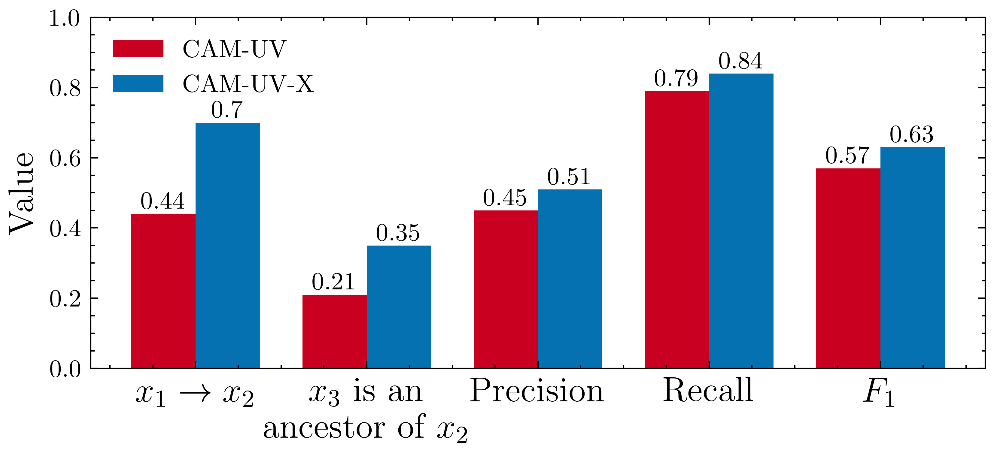
Figure 3: Performance on the graph in Fig. 2a.

Figure 4: Performance on the graph in Fig. 2b.

In Fig. 3, CAM-UV-X is more successful at identifying the visible edge $x_{1}\rightarrow x_{2}$ and at identifying $x_{3}$ as an ancestor of $x_{2}$, and achieves higher precision, recall, and $F_{1}$. In Fig. 4, while the precision of CAM-UV-X is lower, CAM-UV-X is more successful at identifying the non-edge and achieves higher recall.

6.2 Random graph experiment

We investigate CAM-UV-X in simulated causal graphs generated using the popular Barabási–Albert (BA) model [Barabási and Albert, 1999], which produces random graphs with heavy-tailed degree distributions commonly observed in real-world networks [Barabási and Pósfai, 2016]. See Appendix D for an experiment with causal graphs generated from the Erdös-Rényi (ER) model [Erdös and Rényi, 1959], which produces random graphs with binomial degree distributions.

We generate $50$ BA graphs with $40$ nodes, where each node has five children. For each graph, we create data using the same process as in Section 6.1. We then randomly select $10$ variables and create a final dataset of only these $10$ variables. Each dataset contains $500$ samples. We ran the algorithms with confidence levels $\alpha=0.05$, $0.1$, and $0.2$.

Identifying the adjacency matrix. The results are shown in Fig. 5. CAM-UV-X is better in all metrics. See Appendix D for definitions of metrics used in the experiments.

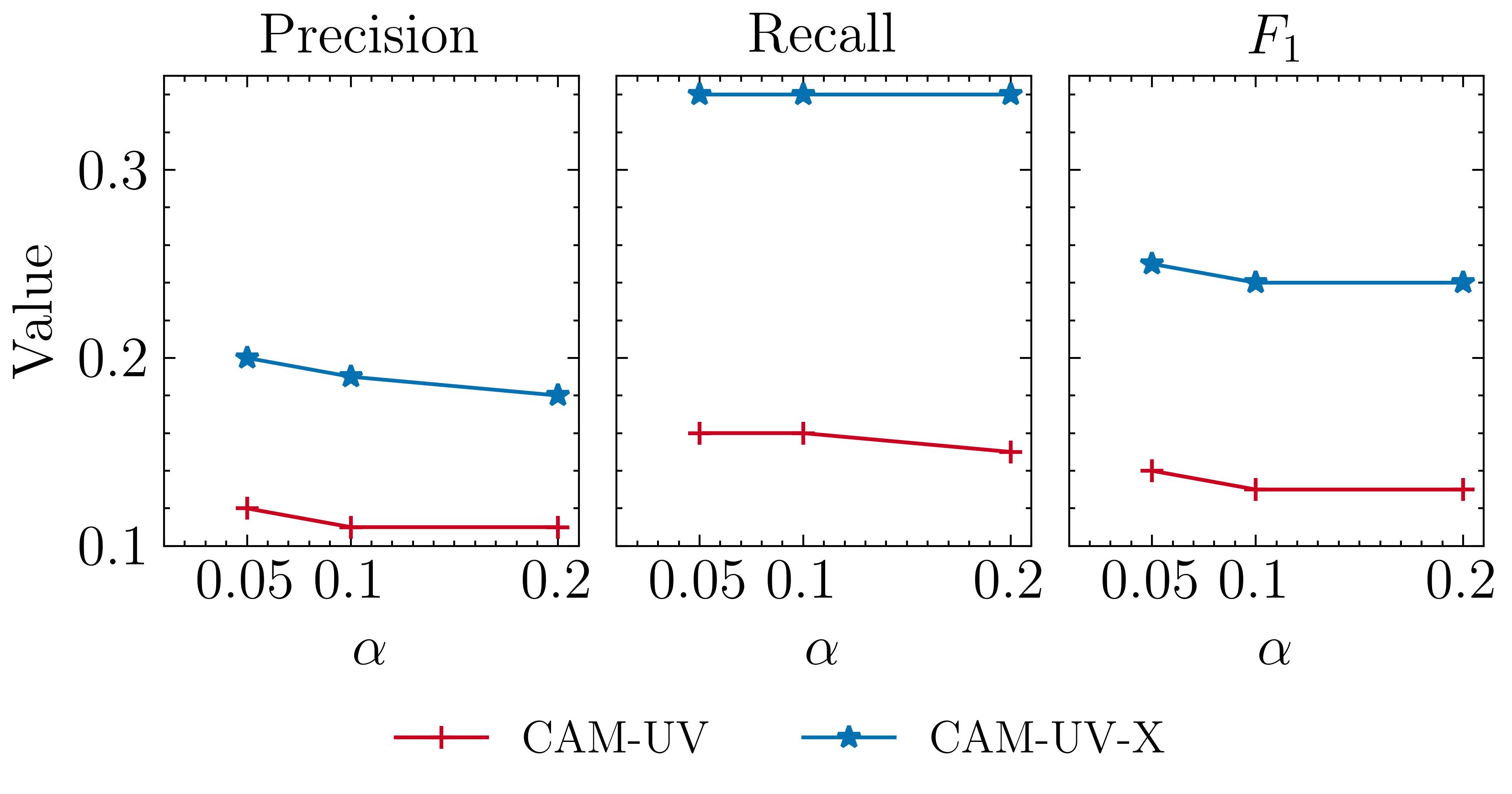
Figure 5: Performance of identifying the adjacency matrix in BA random graphs.

Identifying ancestor relationships. The results are shown in Fig. 6. While precision is similar, CAM-UV-X achieves higher recall and F1.

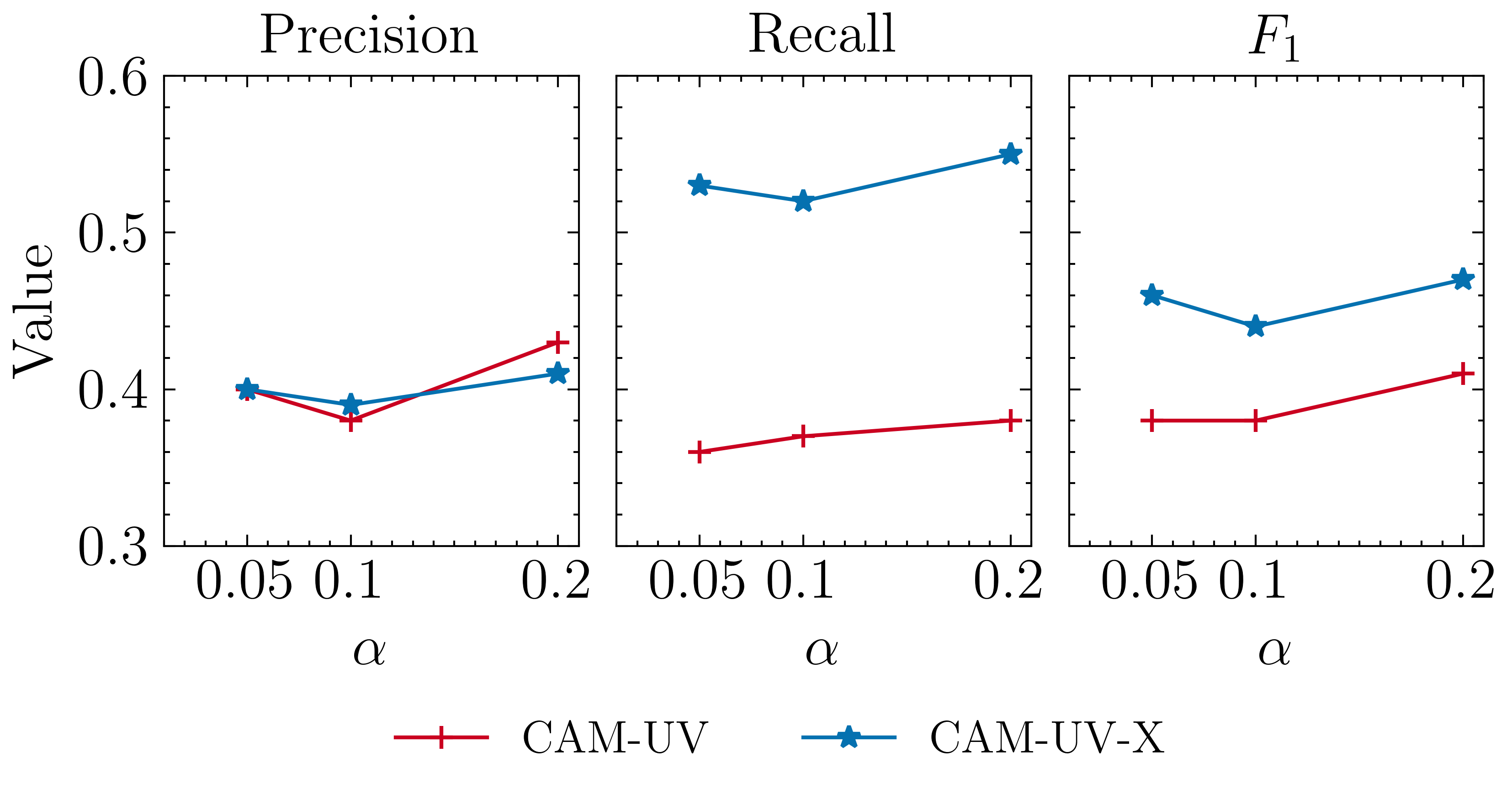
Figure 6: Performance of identifying ancestors in BA random graphs.

Taking into account the results in Appendix D, CAM-UV-X achieves higher recall in both tasks in both graph types, higher F1 in both tasks in BA graphs, higher precision in identifying the adjacency matrix in both graph types, and comparable metric values for other cases.

6.3 FMRI data

We conducted experiments on simulated fMRI data from Smith et al. [2011], which is based on a well-established mathematical model of brain region interactions [Friston et al., 2003]. Specifically, we used their “sim2” dataset, which they describe as one of the most “typical” network scenarios. Using this dataset with ten variables, we randomly chose $k\in[2,3,4,5,6]$ variables, extracted randomly $1000$ samples from those variables, and executed the algorithms. This process was repeated $100$ times for each $k$. The results are shown in Fig. 7.

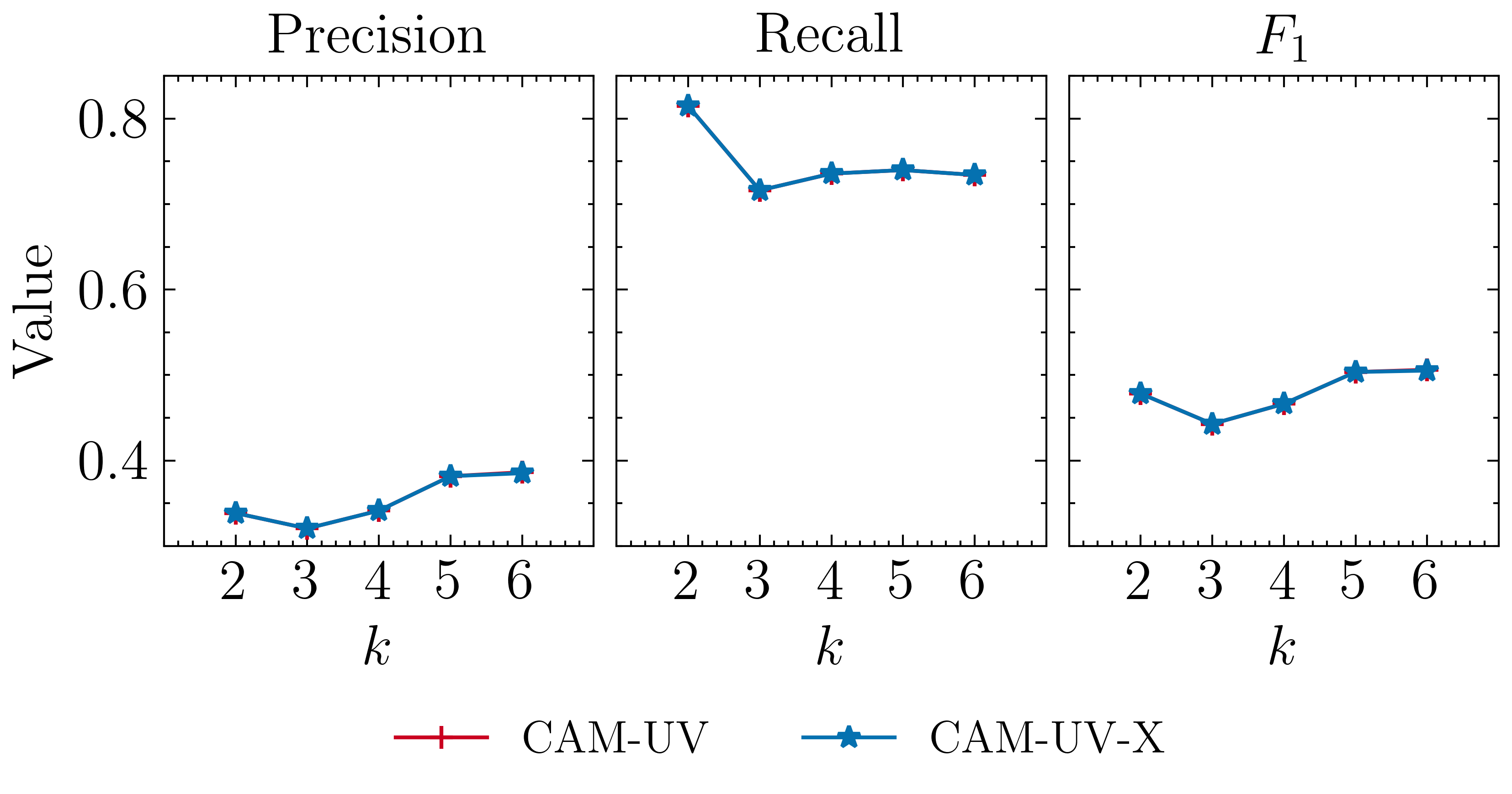
Figure 7: Performance of identifying ancestor relationships in the fMRI dataset.

Overall, CAM-UV-X and CAM-UV performed the same in this dataset.

7 Conclusions

We introduced new identifiability results for parent-child relationships and causal directions in the presence of unobserved backdoor or causal paths in causal additive models. These results stem from a new characterization of the regression sets used in determining independence and a novel approach that combines independence between regression residuals with conditional independence between the original variables.

We introduced the CAM-UV-X algorithm, which integrates these theoretical insights and addresses previously overlooked limitations of the CAM-UV algorithm. Through experiments, we demonstrated that CAM-UV-X effectively resolves these limitations while comparing favorably with CAM-UV.

A systematic investigation to fully characterize what is identifiable in causal additive models with hidden variables remains future work. We believe that our approach of combining independence and conditional independence can yield new identifiability results for other causal models, such as linear non-Gaussian models with hidden variables. Exploring this potential is an avenue for future research.

APPENDIX

Appendix A Assumptions of the CAM-UV model

The CAM-UV model of Maeda and Shimizu [2021] makes the following assumptions.

Assumption 1. If variables $v_{i}$ and $v_{j}$ have terms involving functions of the same external effect $n_{k}$, then $v_{i}$ and $v_{j}$ are mutually dependent, i.e., $(n_{k}\mathrel{\,\not\!\mathrel{\perp\mspace{-9.0mu}\perp}}v_{i})\land(n_{k}\mathrel{\,\not\!\mathrel{\perp\mspace{-9.0mu}\perp}}v_{j})\Rightarrow v_{i}\mathrel{\,\not\!\mathrel{\perp\mspace{-9.0mu}\perp}}v_{j}$.

Assumption 2. When both $x_{i}-G_{i}(M)$ and $x_{j}-G_{j}(N)$ have terms involving functions of the same external effect $n_{k}$, then $x_{i}-G_{i}(M)$ and $x_{j}-G_{j}(N)$ are mutually dependent, i.e., $(n_{k}\mathrel{\,\not\!\mathrel{\perp\mspace{-9.0mu}\perp}}x_{i}-G_{i}(M))\land(n_{k}\mathrel{\,\not\!\mathrel{\perp\mspace{-9.0mu}\perp}}x_{j}-G_{j}(N))\Rightarrow x_{i}-G_{i}(M)\mathrel{\,\not\!\mathrel{\perp\mspace{-9.0mu}\perp}}x_{j}-G_{j}(N)$.

Appendix B Proofs

B.1 Proof of Lemma 3.1

If Eq. (6) is satisfied, it can be shown that, for each $k_{q}$, there is at least a BP/CP not blocked by the set $X\setminus\{x_{k_{q}}\}$, by viewing $x_{k_{q}}$ as an unobserved variable and applying Lemma 2.3.

When Eqs. (7) and (8) are satisfied, $x_{j}$ is a parent of $x_{i}$ and there is no BP/CP not blocked by the set $X$, due to Lemma 2.1. Thus, for each $k_{q}$, there is a UBP/UCP relative to the set $X\setminus\{x_{k_{q}}\}$ that is blocked by $x_{k_{q}}$. This means that $x_{k_{q}}$ is a parent of $x_{j}$ or a parent of $x_{i}$.

B.2 Proof of Lemma 3.2

If Eq. (6) is satisfied, for each $k_{q}$, there is at least a BP/CP not blocked by the set $X\setminus\{x_{k_{q}}\}$, by viewing $x_{k_{q}}$ as an unobserved variable and applying Lemma 2.3.

When Eq. (9) is satisfied, $(x_{i},x_{j})$ is a non-edge and there is no BP/CP not blocked by the set $X$, due to Lemma 2.2. Thus, for each $k_{q}$, there is a UBP/UCP relative to the set $X\setminus\{x_{k_{q}}\}$ that is blocked by $x_{k_{q}}$. This means that $x_{k_{q}}$ is a parent of $x_{j}$ or a parent of $x_{i}$.

B.3 Proof of Lemma 3.3

We prove by contradiction.

1. Suppose there is a backdoor path $x_{i}\leftarrow\cdots\leftarrow v\rightarrow\cdots\rightarrow x_{j}$. Since $x_{k}$ is an ancestor of $x_{i}$, the path $x_{k}\rightarrow\cdots\rightarrow x_{i}\leftarrow\cdots\leftarrow v\rightarrow\cdots\rightarrow x_{j}$ exists. By conditioning on $x_{i}$, which is a collider on this path, the path is open and thus $x_{k}$ and $x_{j}$ cannot be independent. This contradicts the assumption $x_{k}\mathrel{\perp\mspace{-9.0mu}\perp}x_{j}\mid x_{i}$.

2. Suppose $x_{j}$ is an ancestor of $x_{i}$. Since $x_{k}$ is an ancestor of $x_{i}$, the path $x_{k}\rightarrow\cdots\rightarrow x_{i}\leftarrow\cdots\leftarrow x_{j}$ exists. By conditioning on $x_{i}$, which is a collider on this path, the path is open and thus $x_{k}$ and $x_{j}$ cannot be independent. This contradicts the assumption $x_{k}\mathrel{\perp\mspace{-9.0mu}\perp}x_{j}\mid x_{i}$.

Appendix C Step-by-step Execution of CAM-UV on Figs. 2a and b

We work out step-by-step the execution of the CAM-UV algorithm for the graphs in Figs. 2 a and b. We assume that 1) all independence tests are correct, and 2) Line 10 of Algorithm 1 of CAM-UV can correctly find a sink of the set $K$.

C.1 Fig. 2a

• Algorithm 1:

  • Phase 1:

    • $t=2$: The sets $\{x_{1},x_{2}\}$, $\{x_{1},x_{3}\}$, and $\{x_{2},x_{3}\}$ are considered as $K$. The candidate sink $x_{b}$ of $K$ is searched.

      • $K=\{x_{1},x_{3}\}$ or $K=\{x_{2},x_{3}\}$: Since these pairs are invisible, $x_{b}-G_{1}(M_{b}\cup K\setminus\{x_{b}\})$ and $x_{j}-G_{2}(M_{j})$ for $j\in K\setminus\{x_{b}\}$ are not independent, regardless of $x_{b}$. Thus, line 15 will fail since $e\leq\alpha$. There is no change in $M_{i}$.

      • $K=\{x_{1},x_{2}\}$: CAM-UV correctly finds $x_{b}=x_{2}$. However, $x_{b}-G_{1}(M_{b}\cup K\setminus\{x_{b}\})=x_{2}-G_{1}(x_{1})$ and $x_{j}-G_{2}(M_{j})=x_{1}$ is not independent, due to the unblocked backdoor path $x_{1}\leftarrow U_{1}\rightarrow x_{3}\rightarrow x_{2}$. Thus, line 15 will fail since $e\leq\alpha$. There is no change in $M_{i}$.

      $M_{i}$ remains empty for each $i$ and $t$ increases to $3$.

    • $t=3$: $K=\{x_{1},x_{2},x_{3}\}$. The algorithm correctly chooses $x_{b}=x_{2}$. However, $x_{b}-G_{1}(M_{b}\cup K\setminus\{x_{b}\})=x_{2}-G(x_{1},x_{3})$ and $x_{j}-G_{2}(M_{j})=x_{3}$ is not independent, due to the unobserved backdoor path $x_{3}\leftarrow U_{2}\rightarrow x_{2}$. Therefore, line 15 will fail again, since $e\leq\alpha$.

    $M_{i}$ remains empty for each $i$. Phase 1 of the Algorithm 1 ends.

  • Phase 2: Since $M_{i}$ is empty for each $i$, Phase 2 ends.

  Algorithm 1 ends with every $M_{i}$ being empty.

• Algorithm 2: For each pair $(i,j)$, line 5 is satisfied. Therefore, the algorithm concludes every pair is invisible. CAM-UV ends.

The final output is an adjacency matrix where each off-diagonal element is NaN.

C.2 Fig. 2b

• Algorithm 1:

  • Phase 1:

    • $t=2$: The sets $\{x_{1},x_{2}\}$, $\{x_{1},x_{3}\}$, $\{x_{1},x_{4}\}$, $\{x_{2},x_{3}\}$, $\{x_{2},x_{4}\}$, and $\{x_{3},x_{4}\}$ are considered as $K$. The candidate sink $x_{b}$ of $K$ is searched.

      • $K=\{x_{1},x_{2}\}$: Regardless of which $x_{b}$ is, $x_{b}-G_{1}(M_{b}\cup K\setminus\{x_{b}\})=x_{b}-G_{1}(\{x_{1},x_{2}\}\setminus\{x_{b}\})$ and $x_{j}-G_{2}(M_{j})=x_{j}$ for $j\in K\setminus\{x_{b}\}$ are not independent, since there are unblocked BPs/CPs when $x_{3}$ and $x_{4}$ is not added to the regression. Thus, line 15 will fail since $e\leq\alpha$. There is no change in $M_{i}$.

      • The remaining pairs are all invisible. Therefore, $x_{b}-G_{1}(M_{b}\cup K\setminus\{x_{b}\})=x_{b}-G_{1}(K\setminus\{x_{b}\})$ and $x_{j}-G_{2}(M_{j})$ is not independent. Thus, line 15 will fail since $e\leq\alpha$. There is no change in $M_{i}$.

      $M_{i}$ remains empty for each $i$ and $t$ increases to $3$.

    • $t=3$:

      • $K=\{x_{1},x_{2},x_{3}\}$:

        • $x_{b}=x_{2}$: $x_{b}-G_{1}(M_{b}\cup K\setminus\{x_{b}\})=x_{2}-G(x_{1},x_{3})$ and $x_{j}-G_{2}(M_{j})=x_{3}$ is not independent, due to the unobserved backdoor path $x_{3}\leftarrow U_{4}\rightarrow x_{2}$. Therefore, line 15 will fail, since $e\leq\alpha$.

        • $x_{b}=x_{1}$: $x_{b}-G_{1}(M_{b}\cup K\setminus\{x_{b}\})=x_{1}-G(x_{2},x_{3})$ and $x_{j}-G_{2}(M_{j})=x_{3}$ is not independent, due to the unobserved backdoor path $x_{1}\leftarrow U_{1}\rightarrow x_{3}$. Therefore, line 15 will fail, since $e\leq\alpha$.

        • $x_{b}=x_{3}$: $x_{b}-G_{1}(M_{b}\cup K\setminus\{x_{b}\})=x_{3}-G(x_{1},x_{2})$ and $x_{j}-G_{2}(M_{j})=x_{2}$ is not independent, due to the unobserved backdoor path $x_{3}\leftarrow U_{4}\rightarrow x_{2}$. Therefore, line 15 will fail, since $e\leq\alpha$.

      • $K=\{x_{2},x_{3},x_{4}\}$:

        • $x_{b}=x_{2}$: $x_{b}-G_{1}(M_{b}\cup K\setminus\{x_{b}\})=x_{2}-G(x_{3},x_{4})$ and $x_{j}-G_{2}(M_{j})=x_{3}$ is not independent, due to the unobserved backdoor path $x_{3}\leftarrow U_{4}\rightarrow x_{2}$. Therefore, line 15 will fail, since $e\leq\alpha$.

        • $x_{b}=x_{3}$: $x_{b}-G_{1}(M_{b}\cup K\setminus\{x_{b}\})=x_{3}-G(x_{2},x_{4})$ and $x_{j}-G_{2}(M_{j})=x_{2}$ is not independent, due to the unobserved backdoor path $x_{3}\leftarrow U_{4}\rightarrow x_{2}$. Therefore, line 15 will fail, since $e\leq\alpha$.

        • $x_{b}=x_{4}$: $x_{b}-G_{1}(M_{b}\cup K\setminus\{x_{b}\})=x_{4}-G(x_{2},x_{3})$ and $x_{j}-G_{2}(M_{j})=x_{2}$ is not independent, due to the unobserved backdoor path $x_{2}\leftarrow U_{3}\rightarrow x_{4}$. Therefore, line 15 will fail, since $e\leq\alpha$.

      • $K=\{x_{1},x_{3},x_{4}\}$:

        • $x_{b}=x_{1}$: $x_{b}-G_{1}(M_{b}\cup K\setminus\{x_{b}\})=x_{1}-G(x_{3},x_{4})$ and $x_{j}-G_{2}(M_{j})=x_{3}$ is not independent, due to the unobserved backdoor path $x_{3}\leftarrow U_{1}\rightarrow x_{1}$. Therefore, line 15 will fail, since $e\leq\alpha$.

        • $x_{b}=x_{3}$: $x_{b}-G_{1}(M_{b}\cup K\setminus\{x_{b}\})=x_{3}-G(x_{1},x_{4})$ and $x_{j}-G_{2}(M_{j})=x_{1}$ is not independent, due to the unobserved backdoor path $x_{3}\leftarrow U_{1}\rightarrow x_{1}$. Therefore, line 15 will fail, since $e\leq\alpha$.

        • $x_{b}=x_{4}$: $x_{b}-G_{1}(M_{b}\cup K\setminus\{x_{b}\})=x_{4}-G(x_{1},x_{3})$ and $x_{j}-G_{2}(M_{j})=x_{1}$ is not independent, due to the unobserved causal path $x_{1}\rightarrow U_{2}\rightarrow x_{4}$. Therefore, line 15 will fail, since $e\leq\alpha$.

      $M_{i}$ remains empty for each $i$ and $t$ increases to $4$.

    • $t=4$:

      • $K=\{x_{1},x_{2},x_{3},x_{4}\}$.

        • $x_{b}=x_{1}$: $x_{b}-G_{1}(M_{b}\cup K\setminus\{x_{b}\})=x_{1}-G(x_{2},x_{3},x_{4})$ and $x_{j}-G_{2}(M_{j})=x_{3}$ is not independent, due to the unobserved backdoor path $x_{3}\leftarrow U_{1}\rightarrow x_{1}$. Therefore, line 15 will fail, since $e\leq\alpha$.

        • $x_{b}=x_{2}$: $x_{b}-G_{1}(M_{b}\cup K\setminus\{x_{b}\})=x_{2}-G(x_{1},x_{3},x_{4})$ and $x_{j}-G_{2}(M_{j})=x_{3}$ is not independent, due to the unobserved backdoor path $x_{3}\leftarrow U_{4}\rightarrow x_{2}$. Therefore, line 15 will fail, since $e\leq\alpha$.

        • $x_{b}=x_{3}$: $x_{b}-G_{1}(M_{b}\cup K\setminus\{x_{b}\})=x_{3}-G(x_{1},x_{2},x_{4})$ and $x_{j}-G_{2}(M_{j})=x_{1}$ is not independent, due to the unobserved backdoor path $x_{1}\leftarrow U_{1}\rightarrow x_{3}$. Therefore, line 15 will fail, since $e\leq\alpha$.

        • $x_{b}=x_{4}$: $x_{b}-G_{1}(M_{b}\cup K\setminus\{x_{b}\})=x_{4}-G(x_{1},x_{2},x_{3})$ and $x_{j}-G_{2}(M_{j})=x_{2}$ is not independent, due to the unobserved backdoor path $x_{4}\leftarrow U_{3}\rightarrow x_{2}$. Therefore, line 15 will fail, since $e\leq\alpha$.

    $M_{i}$ remains empty for each $i$. Phase 1 of the Algorithm 1 ends.

  • Phase 2: Since $M_{i}$ is empty for each $i$, Phase 2 ends.

  Algorithm 1 ends with every $M_{i}$ being empty.

• Algorithm 2: For each pair $(i,j)$, line 5 is satisfied. Therefore, the algorithm concludes every pair is invisible. CAM-UV ends.

The final output is an adjacency matrix where each off-diagonal element is NaN.

Appendix D Experiments with ER graphs

We generated random graphs from the ER model with 10 observed variables and edge probability $0.2$. We randomly selected 20 pairs of observed variables and introduced a hidden confounder between each pair, and another 20 pairs of observed variables and add a hidden intermediate variable between each pair. We generated $50$ random graphs in this way. For each random graph, we generated $10$ datasets with the same data generating process as in Section 6.1. Each dataset contains $500$ samples. We ran the algorithms with confidence level $\alpha=0.05$, $0.1$, and $0.2$.

Metrics. We define the metrics used in the experiments. $TP$ is the number of true positives. $TN$ is the number of true negatives. $FN$ is the number of false negatives. $FP$ is the number of false positives. In identifying the adjacency matrix $A$, for the case when the estimated $A(i,j)$ is NaN, we add $0.5$ to both $FN$ and $FP$.

The $precision$, $recall$, and $F_{1}$ are calculated as follows. $Precision$ is $TP/(TP+FP)$. $Recall$ is $TP/(TP+FN)$. $F_{1}$ is $2*(precision*recall)/(precision+recall)$.

Identifying the adjacency matrix. The results are shown in Fig. D.1. CAM-UV-X is better than CAM-UV-X in all metrics.

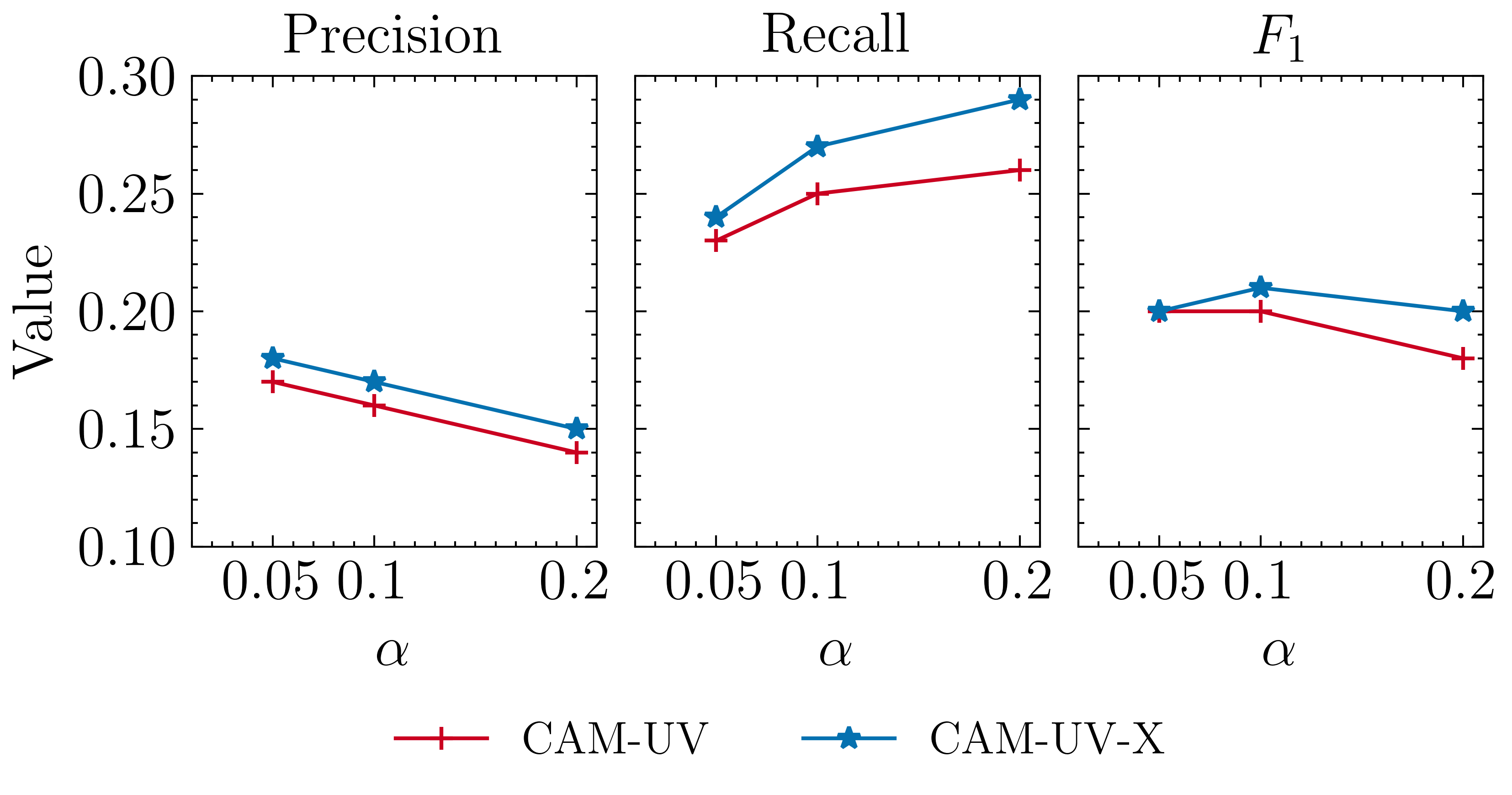
Figure D.1: Performance of identifying the adjacency matrix in ER random graphs.

Identifying ancestor relationships. The results are shown in Fig. D.2. While precision and $F_{1}$ are similar, CAM-UV-X achieved slightly higher recall.

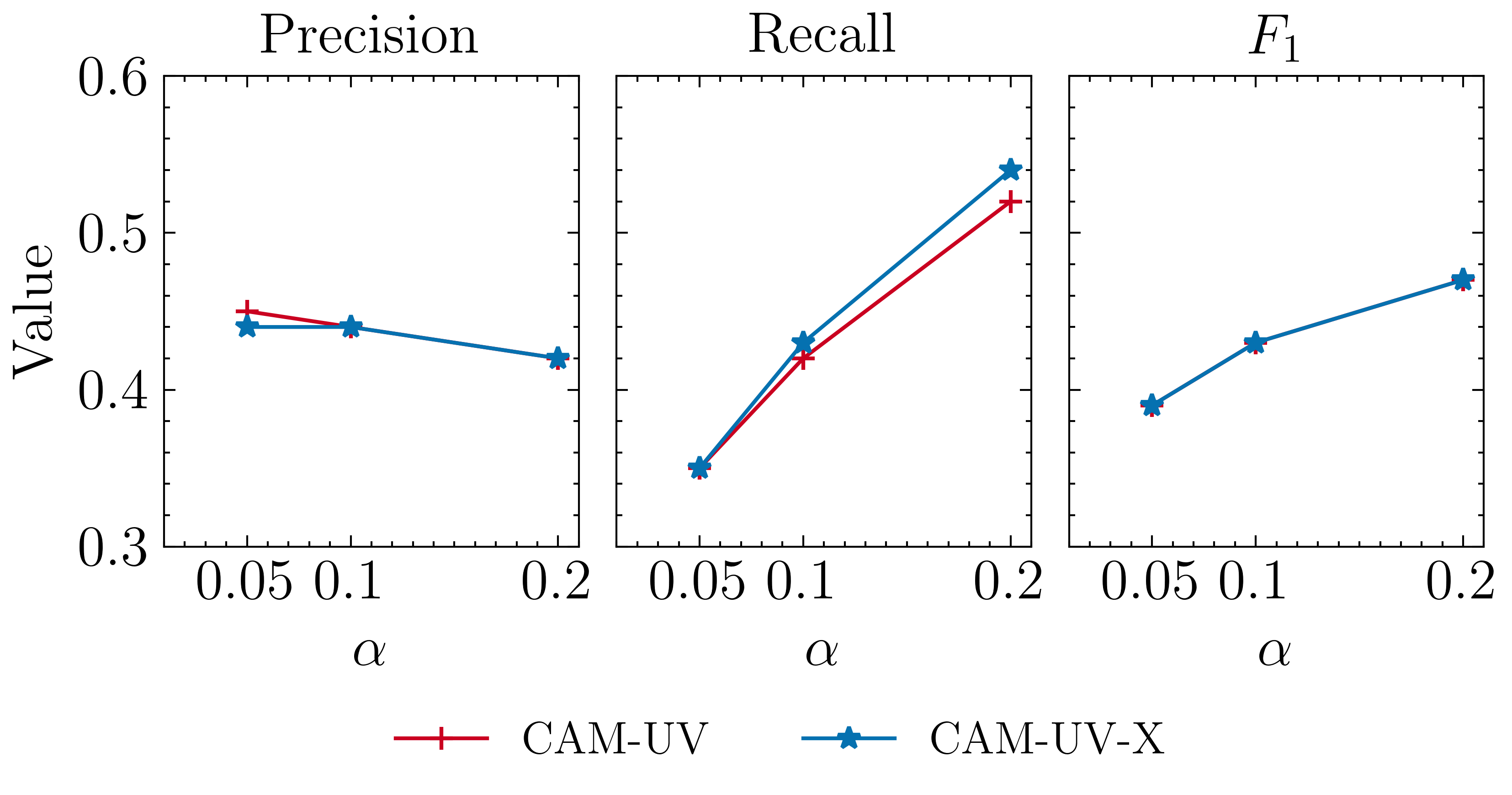
Figure D.2: Performance of identifying ancestors in ER random graphs.