Attention Learning is Needed to Efficiently Learn Parity Function

Abstract

Transformers, with their attention mechanisms, have emerged as the state-of-the-art architectures of sequential modeling and empirically outperform feed-forward neural networks (FFNNs) across many fields, such as natural language processing and computer vision. However, their generalization ability, particularly for low-sensitivity functions, remains less studied. We bridge this gap by analyzing transformers on the $k$-parity problem. Daniely and Malach (NeurIPS 2020) show that FFNNs with one hidden layer and $O(nk^{7}\log k)$ parameters can learn $k$-parity, where the input length $n$ is typically much larger than $k$. In this paper, we prove that FFNNs require at least $\Omega(n)$ parameters to learn $k$-parity, while transformers require only $O(k)$ parameters, surpassing the theoretical lower bound needed by FFNNs. We further prove that this parameter efficiency cannot be achieved with fixed attention heads. Our work establishes transformers as theoretically superior to FFNNs in learning parity function, showing how their attention mechanisms enable parameter-efficient generalization in functions with low sensitivity.

Keywords: transformer, $k$-parity, attention learning, generalization, feature learning

1 Introduction

Transformers (Vaswani et al., 2017), with their self-attention mechanisms, have revolutionized sequential data modeling and have become the backbone for state-of-the-art models in various fields such as computer vision (Dosovitskiy et al., 2020; Carion et al., 2020) and natural language processing (Devlin et al., 2019; Pal et al., 2023). Their empirical superiority over traditional neural networks, including feed-forward neural networks (FFNNs) and recurrent models like LSTMs and RNNs, stems from their ability to dynamically select (or “attend to”) features across long sequences.

The ability of feature selection is particularly critical for low-sensitivity functions, where only a small subset of input tokens decides the output (i.e., the true label $y$ only changes with a subset of size $k$ when the input length $n\gg k$). An example is the $k$-parity problem, where the parameter lower bound for FFNNs to learn this problem is $\Omega(n)$, and the known upper bound is $O(nk^{7}\log k)$, which is proved by Daniely and Malach (2020). Given this inefficiency, architectures that emphasize sparse feature selection are necessary. Transformers have proven to be effective in such tasks through empirical studies (Bhattamishra et al., 2023).

Prior works mainly focused on the expressivity of transformers, i.e., whether specific parameterizations can express some functions, or simulate automatons and Turing machines (Merrill and Sabharwal, 2023, 2024; Bergsträßer et al., 2024). Although expressivity establishes an upper bound on learnability, it does not help to study the generalization ability of transformers; in other words, it does not address whether empirical risk minimization or gradient-based training can converge to the optimal parameterization. Despite empirical evidence that transformers excel at low-sensitivity languages, the learning dynamics and generalization abilities of transformers are not well studied. This gap raises several key questions: Are transformers more parameter efficient than FFNNs in learning sparse functions, specifically on $k$-parity? Can transformers with fixed attention heads also learn $k$-parity efficiently, or is attention learning necessary for such tasks? What are the learning dynamics of these attention heads during gradient descent?

Our contributions.

In this work, we bridge the gap by analyzing the learnability of transformers with the $k$-parity problem. Our contributions are threefold: (i) We show that transformers with $k$ trainable attention heads can learn $k$-parity with only $O(k)$ and parameters. (ii) To show that attention learning is necessary, we prove that approximating $k$-parity with frozen attention heads requires the number of heads $m$ or the norm of the weight of the classification head $\|\theta\|$ to grow polynomially with the input length $n$, more specifically, $\|\theta\|\cdot m^{2}=O(n)$. (iii) We establish that transformers surpass FFNNs in $k$-parity learning in terms of parameter efficiency, reducing the upper bound from $O(nk^{7}\log k)$ (Daniely and Malach, 2020) to $O(k)$.

1.1 Related Works

Expressivity and learnability of transformers.

Prior work has studied the expressivity of transformers through formal languages. Hahn (2020) showed that transformers with hard or soft attention cannot compute parity, a task trivial for vanilla RNNs. This reveals a fundamental limitation of self-attention. Subsequent work (Hao et al., 2022; Merrill and Sabharwal, 2023; Bergsträßer et al., 2024) refined these bounds, restricting the expressivity of transformers within the $\text{FO}(M)$ complexity class. Merrill and Sabharwal (2024) extended the expressivity by augmenting transformers with chain-of-thought reasoning, enabling simulation of Turing machines with time $O(n^{2}+t(n)^{2})$, with $n$ being the input sequence length and $t(n)$ being the number of reasoning steps.

Recent work has also explored the learnability of transformers. Bhattamishra et al. (2023) show transformers under gradient descent favor low-sensitivity functions like $k$-parity compared to LSTMs, but their results are mostly empirical, and they do not provide any theoretical analysis on why transformers can generalize to these functions. A concurrent work by Marion et al. (2025) proves transformers can learn functions where only one input position matters. Although their work theoretically analyses the transformer’s learning dynamic, it is restricted to only one attention head, and a comparison between FFNNs and transformers, especially with respect to parameter efficiency, is not mentioned in the work. This highlights the need for a formal theory of learning and generalization ability of multi-head transformers in low-sensitivity regimes.

Feature learning with neural networks.

The $k$-parity problem is used as a benchmark for analyzing feature learning in neural networks. Prior work shows that two-layer FFNNs trained via gradient descent achieve more efficient feature learning than kernel methods, with the first layer learning meaningful representation as early as the first gradient step (Ba et al., 2022; Shi et al., 2023). This aligns with Daniely and Malach (2020)’s theoretical separation: While linear models on fixed embeddings require an exponential network width to learn this problem, FFNNs with a single hidden layer can achieve a small generalization error using gradient descent with only a polynomial number of parameters. Subsequent analysis (Kou et al., 2024) focuses on lower bounds for the number of iterations needed by stochastic gradient descent to converge. However, these results implicitly require $\Omega(n)$ parameters, raising questions about parameter efficiency and whether other architectures can achieve more effective feature learning with fewer parameters than FFNNs.

2 Problem Statement and Preliminaries

In the remaining part of the paper, the following notations are used. Matrices are denoted by bold capital letters (e.g., $\mathbf{A}$), vectors by bold lowercase letters (e.g., $\mathbf{v}$) and scalars by normal lowercase letters (e.g., $a$). Bold letters with subscripts indicate sequential elements (e.g., $\mathbf{A}_{i}$ is the $i$-th matrix, $\mathbf{v}_{j}$ the $j$-th vector), while normal lowercase letters with subscripts denote specific entries (e.g., $a_{ij}$ is the element in row $i$, column $j$ of $\mathbf{A}$, and $v_{i}$ is the $i$-th scalar component of $\mathbf{v}$). When both subscripts and superscripts are present, the superscript indicates the sequential order, and the subscript indicates the specific entries (e.g., $a^{(i)}_{rl}$ is the entry in row $r$, column $l$ in the $i$-th matrix $\mathbf{A}_{i}$). For logical statements, universal and existential quantifiers are denoted as $\forall x(P(x))$ and $\exists x(P(x))$, indicating that $P(x)$ holds for all $x$ or there exists an $x$ for which $P(x)$ holds, respectively.

2.1 Problem: Learning k-parity

Let $\mathcal{X}=\{0,1\}^{n}$ be the instance space, and $\mathcal{Y}=\{-1,1\}$ be the label space. For any set $\mathcal{B}\subseteq[n]$, we define the parity function $f_{\mathcal{B}}:\mathcal{X}\to\mathcal{Y}$ as $f_{\mathcal{B}}(\mathbf{x})=\left[\prod_{i\in\mathcal{B}}(-1)^{x_{i}}\right]$, i.e., $f_{\mathcal{B}}(\mathbf{x})$ labels $\mathbf{x}$ based on the parity of the sum of the bits in $\mathcal{B}$. We consider learning in a noiseless (and realizable) setting, where data-label pairs have a joint distribution $\mathcal{D}_{\mathcal{B}}$ over $\mathcal{X}\times\mathcal{Y}$ such that $\mathcal{D}_{\mathcal{X}}$ is the uniform distribution over $\mathcal{X}$ and $y=f_{\mathcal{B}}(\mathbf{x})$. We write $\mathcal{D}_{\mathcal{B}}=\mathcal{D}_{\mathcal{X}}\times f_{\mathcal{B}}$. The expected risk of any predictor $h:\mathcal{X}\rightarrow\mathcal{Y}$ over $\mathcal{D}_{\mathcal{B}}$ is defined as: $\mathcal{L}_{\mathcal{D}_{\mathcal{B}}}(h)=\mathbb{E}_{(\mathbf{x},y)\sim\mathcal{D}_{\mathcal{B}}}[\ell(y,h(\mathbf{x}))]$, where we assume that $\ell$ is the squared hinge loss $\ell(y,\hat{y})=\left(\max\{0,1-y\hat{y}\}\right)^{2}$. Given a hypothesis class $\mathcal{H}\subset\mathcal{Y}^{\mathcal{X}}$ and training set $\mathcal{S}\in\bigcup_{N=1}^{\infty}(\mathcal{X}\times\mathcal{Y})^{N}$, we assume that the learning algorithm $f_{\text{learn}}:\bigcup_{N=1}^{\infty}(\mathcal{X}\times\mathcal{Y})^{N}\times\mathcal{H}\rightarrow\mathcal{H}$ is full-batch gradient descent. The algorithm maps any data set $\mathcal{S}$ and initial hypothesis in $\mathcal{H}$ to a learned function through the iterations $h^{(t+1)}=f_{\text{learn}}(h^{(t)},\mathcal{S})$. With this framework, the problem of learning $k$-parity is formally defined as follows:

Definition 1 ($k$-parity learning).

For a known $k$ and unknown $\mathcal{B}\subseteq[n]$ of size $k$, given $N$ labeled samples $\mathcal{S}=\{\mathbf{x}^{(i)},y^{(i)}\}_{i=1}^{N}\sim\mathcal{D}_{\mathcal{B}}^{N}$, the $k$-parity learning problem corresponds to finding a predictor $h\in\mathcal{H}$ such that $\mathcal{L}_{\mathcal{D}_{\mathcal{B}}}(h)<\varepsilon$ for any specified $\varepsilon$. We make further considerations.

The training set $\mathcal{S}$ contains all samples in $\mathcal{X}$, i.e., $\mathcal{L}_{\mathcal{D}_{\mathcal{B}}}(h)$ and its gradients can be computed for any $h$. The $k$-parity problem is learned via full-batch gradient descent $f_{learn}$, i.e., one needs to find an initialization $h^{(0)}\in\mathcal{H}$ such that the iterations $h^{(t)}$ at some stopping satisfies $\mathcal{L}_{\mathcal{D}_{\mathcal{B}}}(h^{(t)})<\varepsilon$.

The assumption of access to expected risk $\mathcal{L}_{\mathcal{D}_{\mathcal{B}}}(h)$ has been made in prior work on learning $k$-parity (Daniely and Malach, 2020) and learning attention in transformers (Marion et al., 2025). We also formalize the notions of expressivity and learnability of hypothesis class $\mathcal{H}$ with respect to $k$-parity.

Definition 2 (Expressivity and learnability of $\mathcal{H}$).

For a specific $\mathcal{B}\subset[n]$, we say that $\mathcal{H}$ can express $\mathcal{D}_{\mathcal{B}}$ if $\mathcal{L}_{\mathcal{D}_{\mathcal{B}}}(\mathcal{H})=\min_{h\in\mathcal{H}}\mathcal{L}_{\mathcal{D}_{\mathcal{B}}}(h)=0$. Furthermore, $\mathcal{H}$ can express $k$-parity if the maximum expected risk over all possible $\mathcal{B}$, i.e., $\max\limits_{|\mathcal{B}|=k}\mathcal{L}_{\mathcal{D}_{\mathcal{B}}}(\mathcal{H})=\max\limits_{|\mathcal{B}|=k}\min\limits_{h\in\mathcal{H}}\mathcal{L}_{\mathcal{D}_{\mathcal{B}}}(h)=0$.

On the other hand, $\mathcal{H}$ can learn the $k$-parity problem with full batch gradient descent $f_{learn}$ if there is a stopping time $t$ such that, for any $|\mathcal{B}|=k$, $\mathcal{L}_{\mathcal{D}_{\mathcal{B}}}(h^{(t)})<\varepsilon$ for a pre-specified small $\epsilon$.

We conclude with the definition of the hypothesis class of one hidden layer FFNN $\mathcal{H}_{\text{FFNN-1}}$ with $q$ neurons and activation function $\sigma$:

$$\mathcal{H}_{\text{FFNN-1}}=\left\{\mathbf{x}\rightarrow\sum_{i=1}^{q}\alpha_{i}\sigma\left(\boldsymbol{\beta}_{i}^{T}\mathbf{x}+b_{i}\right)+b,q\in\mathbb{N},\alpha_{i},b_{i},b\in\mathbb{R},\boldsymbol{\beta}_{i}\in\mathbb{R}^{n}\right\}.$$ (1)

Daniely and Malach (2020) compare the learnability of $\mathcal{H}_{\text{FFNN-1}}$ with $\mathcal{H}_{\Psi}=\{\mathbf{x}\rightarrow\left\langle\Psi(\mathbf{x}),\mathbf{w}\right\rangle\}$, the class of all linear classifiers over some fixed embeddings $\Psi:\mathcal{X}\rightarrow\mathbb{R}^{q}$. They show an exponential separation between $\mathcal{H}_{\text{FFNN-1}}$ and $\mathcal{H}_{\Psi}$, with respect to embedding dimension $q$, by proving that gradient descent on the expected risk $\mathcal{L}_{\mathcal{D}\times f_{\mathcal{B}}}$, for some $\mathcal{D}$ over $\mathcal{X}$, and some initialization $h^{(0)}\in\mathcal{H}_{\text{FFNN-1}}$ can converge to $h^{(t)}$ that approximately learns $k$-parity with polynomial weight norm, regardless of $\mathcal{B}$; while for $\mathcal{H}_{\Psi}$, the expected risk $\max_{|\mathcal{B}|=k}\mathcal{L}_{\mathcal{D}_{\mathcal{B}}}(\mathcal{H}_{\Psi})$ is always non-trivial unless the weight norm $\|\mathbf{w}\|_{2}$ or the embedding dimension $q$ grows exponentially with $n$. In this work, we compare the expressivity and learnability of $\mathcal{H}_{\text{FFNN-1}}$ with the class of transformer defined below.

2.2 Multi-Head Single-Attention-Layer Transformer

We consider the transformer illustrated in Figure 1 to learn $k$-parity. It contains a single encoding layer with $m$ attention heads, where each head is parameterized by $\mathbf{A}_{i}\in\mathbb{R}^{2d\times 2d}$ (for a fixed embedding dimension $2d$), and an FFNN with one hidden layer parameterized by $\theta$. The transformer will process a binary input $\mathbf{x}=x_{1}\dots x_{n}$ of length $n$ through the following layers:

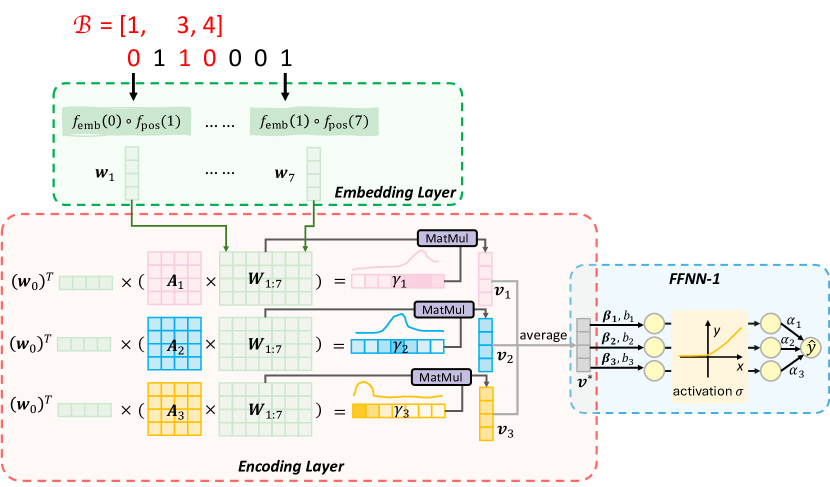
Figure 1: The architecture of the transformer and the example workflow to classify the parity of some given input. Given a binary string that consists of $7$ tokens as input, the embedding layer (in green) will embed each token into a concatenation of a positional embedding and a token embedding $\mathbf{w}_{j}=f_{\text{pos}}(j)\circ f_{\text{emb}}(x_{j})$. An extra token embedding $\mathbf{w}_{0}$ will be prepended as the embedding of the CLS token. In the encoding layer (in red), each attention head $i$ will calculate attention scores $\boldsymbol{\gamma_{i}}$ for all of the seven embeddings with softmax. Then, each head will calculate its own vector $\mathbf{v}_{i}$ by taking the sum of the $7$ embeddings weighted by its own attention score: $\mathbf{v}_{i}=\sum_{j=1}^{n}\gamma^{(i)}_{j}\cdot\mathbf{w}_{j}$. These vectors will then be averaged into an attention vector $\mathbf{v}^{*}=\frac{1}{m}\sum_{i\in[m]}\mathbf{v}_{i}$, which will be the input of the two-layer feed-forward neural network (in blue).

Embedding Layer.

The input to this layer is the $n$ tokens $x_{1},\dots,x_{n}$ separately, and the output is $(n+1)$ embeddings, each of dimension $2d$, for the $n$ tokens and a prepended classification token (CLS). For each token $x_{j}\in\{0,1\}$, a word embedding $f_{\text{embed}}(x_{j})\in\mathbb{R}^{d}$ and a positional embedding $f_{\text{pos}}(j)\in\mathbb{R}^{d}$ will be generated and concatenated into the final token embedding $\mathbf{w}_{j}=f_{\text{embed}}(x_{j})\circ f_{\text{pos}}(j)\in\mathbb{R}^{2d}$, where $\circ$ is the concatenation symbol. Later we show that it suffices to use a fixed $d$, independent of $n$ or $k$, for learning $k$-parity (we use $d=2$). In addition, a CLS $x_{0}$ is prepended to the input sequence, with a token embedding $\mathbf{w}_{0}\in\mathbb{R}^{2d}$.

Encoding Layer.

The input to this layer is the $(n+1)\times 2d$ token embeddings, and the output is $m$ attention vectors, each with dimension $2d$, where $m$ is the number of attention heads. Each head is parameterized by an attention matrix $\mathbf{A}_{i}$. Unlike standard attention Vaswani et al. (2017), where token embeddings are partitioned into $m$ parts for each head, we allow each head to operate on the full embedding. Each head $\mathbf{A}_{i}$ computes a correlation score between $\mathbf{w}_{j}$ and $\mathbf{w}_{0}$: $s^{(i)}_{j}=(\mathbf{w}_{0})^{T}\mathbf{A}_{i}\mathbf{w}_{j}$, which is then normalized using a softmax function: $\gamma_{j}^{(i)}=\frac{\exp\left({s^{(i)}_{j}}/{\tau}\right)}{\sum_{p=1}^{n}\exp\left({s^{(i)}_{p}}/{\tau}\right)}$, where $0<\tau\leq 1$ is the temperature controlling the smoothness of softmax. With this, each head computes $\mathbf{v}_{i}=\sum\limits_{j=1}^{n}\gamma^{(i)}_{j}\mathbf{w}_{j}$, which is averaged across all heads into an attention vector $\mathbf{v}^{*}=\frac{1}{m}\sum\limits_{i=1}^{m}\mathbf{v}_{i}$.

Classification Head.

The classification head is an FFNN with one hidden layer. It takes $\mathbf{v}^{*}$ from the encoding layer and outputs a prediction $\hat{y}\in\mathbb{R}$. This layer corresponds to the class $\mathcal{H}_{\textbf{FFNN-1}}$ in (1) with $q$ neurons and the activation is $\sigma(x)=\frac{x+\sqrt{x^{2}+b_{\sigma}}}{2},b_{\sigma}>0$. For convenience, we denote all trainable parameters in this module by $\theta=(\boldsymbol{\beta},b_{i},\boldsymbol{\alpha},b)$, and use $\Theta$ for the parameter space of the FFNN.

We denote the output of the overall transformer as $\hat{y}=h_{\mathbf{A}_{1:m},\theta}(\mathbf{x})$. The hypothesis class represented by the transformer architecture is $\mathcal{H}_{\text{transformer}}=\left\{\mathbf{x}\rightarrow h_{\mathbf{A}_{1:m},\theta}(\mathbf{x}),\mathbf{A}_{i}\in\mathbb{R}^{2d\times 2d},\theta\in\Theta\right\}$. In this paper, we study two subsets of $\mathcal{H}_{\text{transformer}}$: (i) $\mathcal{H}_{\bar{\theta}}=\{\mathbf{x}\rightarrow h_{\mathbf{A}_{1:m},\bar{\theta}}(\mathbf{x}),\mathbf{A}_{i}\in\mathbb{R}^{2d\times 2d}\}$, where the FFNN has $q=k$ neurons, parameters in the FFNN is frozen as $\bar{\theta}$ and only the weight matrices for attention heads are trainable; (ii) $\mathcal{H}_{\bar{\mathbf{A}}}=\{\mathbf{x}\rightarrow h_{\bar{\mathbf{A}},\theta}(\mathbf{x}),\theta\in\Theta\}$, where the weight matrices of the attention heads are fixed as $\bar{\mathbf{A}}$ and only the parameters in the FFNN is trainable.

3 How many parameters do different models need to express and learn k-parity?

Our main result, in the next section, states: if attention heads are trained, then transformers with only $O(k)$ trainable parameters can learn $k$-parity. Before stating this result, we present a broad perspective that helps to distinguish the expressive power and the learning ability of a hypothesis class with respect to the $k$-parity problem (see Definition 2). This can be formalized through the parameter efficiency or, more technically, the number of edges in the computation graph of functions needed to model $k$-parity. For a fixed $\mathcal{B}\subseteq[n],|\mathcal{B}|=k$, one naturally needs a computation graph with $k$ edges, corresponding to the $k$ edges that connect the $k$ bits/tokens $\{x_{i}\}_{i\in\mathcal{B}}$ to a node that computes $f_{\mathcal{B}}(\mathbf{x})$. The natural question related to expressivity is whether one can construct hypothesis classes, using FFNNs or transformers, where the computation graph of each predictor has only $O(k)$ edges. Proposition 3 shows that is possible, naïvely suggesting that it is possible to learn $k$-parity using only models with $O(k)$ parameters, where each parameter corresponds to one edge of the FFNN or transformer model. We restrict the data distribution to $\mathcal{D}_{\mathcal{B}}=\mathcal{D}_{\mathcal{X}}\times f_{\mathcal{B}}$, with $\mathcal{D}_{\mathcal{X}}$ uniform, but the results in this section also hold for other marginal distributions and noisy labels.

Proposition 3 (Number of parameters needed by FFNNs and transformers to express $k$-parity).

Assume $k\leq n$. There exists a hypothesis class $\mathcal{H}_{\text{FFNN-}1^{k}}\subseteq\mathcal{H}_{\text{FFNN-}1}$ that expresses $k$-parity, and each $h\in\mathcal{H}_{\text{FFNN-}1^{k}}$ has exactly $k$ neurons and $2k+2$ distinct parameters. Furthermore, there exists a class $\mathcal{H}^{\prime}_{\bar{\theta}}\subseteq\mathcal{H}_{\text{transformer}}$ that expresses $k$-parity, and each $h\in\mathcal{H}^{\prime}_{\bar{\theta}}$ has exactly $k$ heads in the encoding layer, $k$ neurons in classification layer, and overall $18k+2$ distinct parameters.

Proof  We first prove that FFNNs with $O(k)$ parameters, or edges in the computation graph, are sufficient to express $k$-parity. The main idea is to construct a subclass by selecting a $h\in\mathcal{H}_{\text{FFNN-}1}$ for each $k$-parity function $f_{\mathcal{B}}$. Construct the following hypothesis class $\mathcal{H}_{\text{FFNN-1}^{k}}\subseteq\mathcal{H}_{\text{FFNN-}1}$:

$$\mathcal{H}_{\text{FFNN-1}^{k}}=\bigcup_{B\in\binom{[n]}{k}}\{h_{B}\},\quad h_{B}(\mathbf{x})=1+\sum_{j=1}^{k}(-1)^{j}\cdot(8j-4)\cdot\text{ReLU}\left(\sum_{p\in B}x_{p}+0.5-j\right),$$

where $\binom{[n]}{k}$ denotes the set of all different subsets of $[n]$ with k elements, and each $h_{B}$ outputs the parity of the sum of bits in $B$. Then for any $\mathcal{B}$, we have $\mathcal{L}_{\mathcal{D}_{\mathcal{B}}}(\mathcal{H}_{\text{FFNN-1}^{k}})=0$, i.e, $\mathcal{H}_{\text{FFNN-1}^{k}}$ expresses $k$-parity, and all models in $\mathcal{H}_{\text{FFNN-1}^{k}}$ have only $k$ neurons and $2k+2$ parameters.

We next construct transformers with $18k+2$ parameters that can express $k$-parity. Consider $\mathcal{H}^{\prime}_{\bar{\theta}}\subseteq\mathcal{H}_{\bar{\theta}}\subseteq\mathcal{H}_{\text{transformer}}$, consisting of $\binom{n}{k}$ different transformers with $k$ heads, each with different fixed attention matrices. The classification head in $\mathcal{H}^{\prime}_{\bar{\theta}}$ is fixed as $\bar{\theta}$:

$$\mathcal{H}^{\prime}_{\bar{\theta}}=\bigcup_{B\in\binom{[n]}{k}}\left\{h_{\bar{\theta},\mathbf{A}^{B}_{1:k}}\right\},\mathbf{A}^{B}_{i}\text{ s.t. }a_{13}=\sin\frac{2\pi B_{i}}{n},a_{14}=\cos\frac{2\pi B_{i}}{n},0\text{ otherwise};$$ (2)

$$h_{\bar{\theta},\mathbf{A}^{B}_{1:k}}(\mathbf{x})=1+\sum_{i=1}^{k}(-1)^{i}\cdot(8i-4)\cdot\sigma\left(\left\langle[k,0,0,0],\mathbf{v}^{*}(\mathbf{A}^{B}_{1:k})\right\rangle+0.5-i\right),$$

where $B_{i}$ is the $i$-th element in set $B$ and $\mathbf{v}^{*}(\mathbf{A}^{B}_{1:k})$ denotes the attention vector generated with attention matrices $\mathbf{A}^{B}_{1:k}$. Here we use the token embeddings $\mathbf{w}_{j}=f_{\text{embed}}(x_{j})\circ f_{\text{pos}}(j)\in\mathbb{R}^{4}$, where:

$$f_{\text{emb}}(0)=[0,1]^{T},f_{\text{emb}}(1)=[1,0]^{T},f_{\text{pos}}(i)=\left[\sin\frac{2\pi i}{n},\cos\frac{2\pi i}{n}\right]^{T},\mathbf{w}_{0}=[1,0,0,0]^{T}.$$ (3)

Therefore, $\mathbf{A}^{B}_{i}$ will align with the direction of $B_{i}$, and $v^{*}_{1}=\frac{1}{k}\sum_{p\in B}x_{p}$. Therefore, it holds that $\max_{|\mathcal{B}|=k}\mathcal{L}_{\mathcal{D}_{\mathcal{B}}}(h_{\bar{\theta},\mathbf{A}^{\mathcal{B}}_{1:k}})=0$. And transformers in $\mathcal{H}^{\prime}_{\bar{\theta}}$ only have $18k+2$ parameters.  

Proposition 3 shows that the finite subclasses of FFNNs, $\mathcal{H}_{\text{FFNN-1}^{k}}$, or transformers, the hypothesis class $\mathcal{H}^{\prime}_{\bar{\theta}}$, can express $k$-parity. However, learning with gradient descent is not possible on these classes due to the discrete space. While for transformers one can learn over a larger class $\mathcal{H}_{\bar{\theta}}$ (see next section), but $\mathcal{H}_{\text{FFNN-1}^{k}}$ does not have a common parameter space of dimension $O(k)$ over which one can apply gradient descent. The next result proves a stronger result that to learn $k$-parity with FFNNs via gradient descent, one needs at least $\Omega(n)$ trainable parameters.

Proposition 4 (Number of parameters needed by FFNNs to learn $k$-parity).

With gradient descent, $\Omega(n)$ number of parameters is the required lower bound for FFNNs to learn $k$-parity.

Proof  While we proved that $\mathcal{H}_{\text{FFNN-1}^{k}}$ can express $k$-parity, this class contains functions with pairwise unique computational graphs. Consequently, gradient descent with functions with the same computation maps as any $h\in\mathcal{H}_{\text{FFNN-1}^{k}}$ as initialization cannot converge to any other function in the same hypothesis class. So we have to find another hypothesis class with more parameters. We assume $\mathcal{H}^{\prime}\subseteq\mathcal{H}_{\text{FFNN-1}}$ is any hypothesis class, where there exists $h^{(0)}$, such that for any $|\mathcal{B}|=k$, gradient descent over $\mathcal{D}_{\mathcal{B}}$ will converge on $h^{(t)}$, such that $\mathcal{L}_{\mathcal{D}_{\mathcal{B}}}(h^{(t)})<\varepsilon$. Note that for any initialization $h^{(0)}$, gradient descent will not change the edges and nodes in its computation map. Consider any $h^{(0)}\in\mathcal{H}_{\text{FFNN-}1}$, where its computation map doesn’t have an outgoing edge for some $i\in[n]$, then the computation map of $h^{(t)}$ does not have an outgoing edge for some $i\in[n]$ as well. Define the function $f_{\text{flip-}p}(\mathbf{x})=x_{1}\dots(1-x_{p})\dots x_{n}$. When $i\in\mathcal{B}$, we have $h^{(t)}(\mathbf{x})=h^{(t)}(f_{\text{flip-}i}(\mathbf{x}))$ for any $\mathbf{x}\in\mathcal{X}$, so $\mathcal{L}_{\mathcal{D}_{\mathcal{B}}}(h^{(t)})=1$. Hence for FFNNs, the lower bound on the number of parameters required to learn the $k$-parity problem with an unknown parity set is $\Omega(n)$.  

Propositions 3 and 4 show that, while FFNNs with $O(k)$ parameters can express $k$-parity, they require $\Omega(n)$ parameters to learn it, which is not ideal in typical scenarios where $n\gg k$. However, since $\mathcal{H}_{\bar{\theta}}$ defined earlier satisfies $\mathcal{H}^{\prime}_{\bar{\theta}}\subseteq\mathcal{H}_{\bar{\theta}}\subseteq\mathcal{H}_{\text{transformer}}$, it can express $k$-parity and has a continuous parameter space of dimension $O(k)$ (the learnable attention matrices $\mathbf{A}_{1:k}$). This naturally raises the question of whether $\mathcal{H}_{\bar{\theta}}$ can learn $k$-parity via gradient descent, which we answer next.

4 Main Results: Importance of attention learning to learn k-parity

Our main results are two-fold: We first proved that the hypothesis class $\mathcal{H}_{\bar{\theta}}\subseteq\mathcal{H}_{\text{transformer}}$ of transformers with $k$ learnable attention heads and FFNN-1 parameterized by $\bar{\theta}$ as classification head can approximate any $\mathcal{D}_{\mathcal{B}}$ with $|\mathcal{B}|=k$, which require only $O(k)$ parameters. To show attention learning is crucial to learn $k$-parity, we prove that $\mathcal{H}_{\bar{\mathbf{A}}}\subseteq\mathcal{H}_{\text{transformer}}$, where only the FFNN-1 is learnable, cannot learn the $k$-parity problem unless $\|\boldsymbol{\alpha}\|\|\boldsymbol{\beta}\|m^{2}=O(n)$, with $\|\boldsymbol{\alpha}\|$ and $\|\boldsymbol{\beta}\|$ being the weight norms for the output layer and the hidden layer, $m$ being number of frozen attention heads.

For Theorem 1, we use the token and position embeddings specified in (3). The entries of each $\mathbf{A}^{(0)}_{i},i\in[k]$ is initialized as:

$$\omega_{i}\sim\textbf{Unif}([0,2\pi]),\quad a_{13}=\cos\omega_{i},\quad a_{14}=\sin\omega_{i},\text{ 0 otherwise}.$$

Furthermore, we fix the parameters of the classification head as $\bar{\theta}$ as in (2). For simplicity, from now on we use $\mathcal{L}_{\mathcal{D}_{\mathcal{B}}}(\mathbf{A}_{1:k})$ to denote $\mathcal{L}_{\mathcal{D}_{\mathcal{B}}}(h_{\bar{\theta},\mathbf{A}_{1:k}})$. These heads are then updated over the expected risk with gradient descent: $\mathbf{A}_{1:k}^{(t+1)}=\mathbf{A}_{1:k}^{(t)}-\eta\nabla\mathcal{L}_{\mathcal{D}_{\mathcal{B}}}\left(\mathbf{A}_{1:k}^{(t)}\right).$

The next theorem shows that if the attention heads are trainable, transformers can learn $k$-parity with only $k$ heads on top of the FFNN-1 parameterized by $\bar{\theta}$.

Theorem 5 (Transformers with learnable attention heads can learn $k$-parity).

Training the $k$ attention heads on top of FFNN-1 parameterized by $\bar{\theta}$ converges to the optimal risk $\mathcal{L}_{\mathcal{D}_{\mathcal{B}}}=0$ (with attention head specified in (2)), i.e., with some $0<c<1$, it holds that:

$$\mathcal{L}_{\mathcal{D}_{\mathcal{B}}}\left(\mathbf{A}_{1:k}^{(t)}\right)\leq c^{t}\cdot\mathcal{L}_{\mathcal{D}_{\mathcal{B}}}\left(\mathbf{A}_{1:k}^{(0)}\right).$$

Since the loss at initialization is 1, $\forall\varepsilon>0$, when $t>\frac{|\ln\epsilon|}{-\ln c}$, we have that $\mathcal{L}_{\mathcal{D}_{\mathcal{B}}}\left(\mathbf{A}_{1:k}^{(t)}\right)<\varepsilon$.

Proof Sketch. We provide an outline of the proof in this sketch, while the detailed proofs of the lemmas can be found in Appendix A. Note that for any head $i\in[k]$, there is no gradient update for any entry $a^{(i)}_{rl}$ when $r\neq 1$ and $l\notin\{3,4\}$. In the following analysis, the notation $\mathbf{A}_{1:k}$ refers to the vectorization $[a^{(1)}_{13},a^{(1)}_{14},\dots,a^{(k)}_{13},a^{(k)}_{14}]^{T}.$ First, we establish the smoothness (the Lipschitzness of the gradient) of the expected risk. To achieve this, we take a step back and show that $\hat{y}$ is smooth.

Lemma 6 (smoothness of $\hat{y}$).

$\hat{y}$ is $B$-smooth w.r.t. $\mathbf{A}_{1:k}$, i.e.:

$$\left\|\nabla\hat{y}(\mathbf{A}_{1:k})-\nabla\hat{y}(\mathbf{A}^{\prime}_{1:k})\right\|\leq B\left\|\mathbf{A}_{1:k}-\mathbf{A}^{\prime}_{1:k}\right\|$$

Then, on top of the previous lemma, we can prove the smoothness of the expected risk w.r.t. $\mathbf{A}_{1:k}$.

Lemma 7 (smoothness of $\mathcal{L}_{\mathcal{D}}$).

Denote the Lipschitz constant of $\hat{y}$ and $\hat{y}\cdot\nabla\hat{y}(\mathbf{A}_{1:k})$ by $l_{1}$ and $l_{2}$, and the upper bound of $\|\nabla\hat{y}(\mathbf{A}_{1:k})\|$ by $C$ (Refer to Lemma 15 and Lemma 16), it holds that:

$$\left\|\nabla\mathcal{L}_{\mathcal{D}_{\mathcal{B}}}(\mathbf{A}_{1:k})-\nabla\mathcal{L}_{\mathcal{D}_{\mathcal{B}}}(\mathbf{A}^{\prime}_{1:k})\right\|\leq\max\{2l_{1}C,2(l_{2}+B)\}\left\|\mathbf{A}_{1:k}-\mathbf{A}^{\prime}_{1:k}\right\|$$

Proof  Since the smoothness of the loss $\ell$ will propagate into the smoothness of the expected risk $\mathcal{L}_{\mathcal{D}_{\mathcal{B}}}$, to prove this lemma, it is sufficient to show that:

$$\left\|\nabla\ell(\mathbf{A}_{1:k})-\nabla\ell(\mathbf{A}^{\prime}_{1:k})\right\|\leq\max\{2l_{1}C,2(l_{2}+B)\}\left\|\mathbf{A}_{1:k}-\mathbf{A}^{\prime}_{1:k}\right\|$$ (4)

Take the gradient of $\mathbf{A}_{1:k}$ and $\mathbf{A}^{\prime}_{1:k}$ w.r.t. $\ell$, and we can write the LHS of (4) as:

$$\left\|\nabla\ell(\mathbf{A}_{1:k})-\nabla\ell(\mathbf{A}^{\prime}_{1:k})\right\|=\left\|\frac{\partial\ell}{\partial\hat{y}}(\mathbf{A}_{1:k})\cdot\nabla\hat{y}(\mathbf{A}_{1:k})-\frac{\partial\ell}{\partial\hat{y}}(\mathbf{A}^{\prime}_{1:k})\cdot\nabla\hat{y}(\mathbf{A}^{\prime}_{1:k})\right\|.$$

Suppose w.l.o.g. that $y=1$, we have $\frac{\partial\ell}{\partial\hat{y}}=0$ when $\hat{y}\geq 1$ and $\frac{\partial\ell}{\partial\hat{y}}=2(\hat{y}-1)$ when $\hat{y}<1$. Afterwards, we consider LHS of (4) in the following cases:

(i) When $\hat{y}(\mathbf{A}_{1:k}),\;\hat{y}(\mathbf{A}^{\prime}_{1:k})\geq 1$. LHS $=0$, and $0\leq\max\{2l_{1}C,2(l_{2}+B)\}\left\|\mathbf{A}_{1:k}-\mathbf{A}^{\prime}_{1:k}\right\|$ holds.

(ii) When $\hat{y}(\mathbf{A}_{1:k})\leq 1\leq\hat{y}(\mathbf{A}^{\prime}_{1:k})$ or $\hat{y}(\mathbf{A}_{1:k})\leq 1\leq\hat{y}(\mathbf{A}^{\prime}_{1:k})$. Rearranging the LHS of (4):

$$\begin{split}\left\|\nabla\ell(\mathbf{A}_{1:k})-\nabla\ell(\mathbf{A}^{\prime}_{1:k})\right\|&=\left\|2(\hat{y}(\mathbf{A}_{1:k})-1)\nabla\hat{y}(\mathbf{A}_{1:k})\right\|\leq\left\|2(\hat{y}(\mathbf{A}_{1:k})-1)\right\|\left\|\nabla\hat{y}(\mathbf{A}_{1:k})\right\|\\ &\leq\left\|2(\hat{y}(\mathbf{A}_{1:k})-\hat{y}(\mathbf{A}^{\prime}_{1:k}))\right\|\left\|\nabla\hat{y}(\mathbf{A}_{1:k})\right\|\leq 2l_{1}C\left\|\mathbf{A}_{1:k}-\mathbf{A}^{\prime}_{1:k}\right\|\end{split}$$

(iii) When $\hat{y}(\mathbf{A}_{1:k})\leq 1,\hat{y}(\mathbf{A}^{\prime}_{1:k})\leq 1$, LHS of (4) becomes:

$$\begin{split}\left\|\nabla\ell(\mathbf{A}_{1:k})-\nabla\ell(\mathbf{A}^{\prime}_{1:k})\right\|&=\left\|2\hat{y}(\mathbf{A}_{1:k})\nabla\hat{y}(\mathbf{A}_{1:k})-2\hat{y}(\mathbf{A}^{\prime}_{1:k})\nabla\hat{y}(\mathbf{A}^{\prime}_{1:k})-2(\nabla\hat{y}(\mathbf{A}_{1:k})-\nabla\hat{y}(\mathbf{A}^{\prime}_{1:k}))\right\|\\ &\leq 2\left\|\hat{y}(\mathbf{A}_{1:k})\nabla\hat{y}(\mathbf{A}_{1:k})-\hat{y}(\mathbf{A}^{\prime}_{1:k})\nabla\hat{y}(\mathbf{A}^{\prime}_{1:k})\right\|+2\left\|\nabla\hat{y}(\mathbf{A}_{1:k}-\nabla\hat{y}(\mathbf{A}^{\prime}_{1:k})\right\|\\ &\leq 2(l_{2}+B)\left\|\mathbf{A}_{1:k}-\mathbf{A}^{\prime}_{1:k}\right\|\end{split}$$

Hence $\ell$ is $\max\{2l_{1}C,2(l_{2}+B)\}$-smooth, so $\mathcal{L}_{\mathcal{D}_{\mathcal{B}}}$ is also $\max\{2l_{1}C,2(l_{2}+B)\}$-smooth.  
Next, we prove that the risk also satisfies the $\mu$-PL condition (Polyak, 1963):

Lemma 8 ($\mu$-PL condition on the expected risk).

The squared 2-norm of the gradient of the expected risk is lower bounded by the expected risk times by factor $\mu$:

$$\frac{1}{2}\left\|\nabla\mathcal{L}_{\mathcal{D}_{\mathcal{B}}}(\mathbf{A}_{1:k})\right\|^{2}_{2}\geq\mu\cdot\mathcal{L}_{\mathcal{D}_{\mathcal{B}}}(\mathbf{A}_{1:k})$$ (5)

Proof  Consider the LHS of (5), it holds that:

$$\|\nabla\mathcal{L}_{\mathcal{D}_{\mathcal{B}}}(\mathbf{A}_{1:k})\|^{2}_{2}=\sum_{i=1}^{k}\left[\left(\frac{\partial\mathcal{L}_{\mathcal{D}_{\mathcal{B}}}}{\partial a^{(i)}_{13}}\right)^{2}+\left(\frac{\partial\mathcal{L}_{\mathcal{D}_{\mathcal{B}}}}{\partial a^{(i)}_{14}}\right)^{2}\right]$$

$$= \sum_{i=1}^{k}\left[\mathbb{E}\left[\frac{\partial\ell(y,\hat{y}(\mathbf{A}_{1:k}))}{\partial a^{(i)}_{13}}\right]^{2}+\mathbb{E}\left[\frac{\partial\ell(y,\hat{y}(\mathbf{A}_{1:k}))}{\partial a^{(i)}_{14}}\right]^{2}\right]$$

$$= \sum_{i=1}^{k}\left[\frac{1}{2^{2n}}\left(\sum_{N=1}^{2^{n}}\frac{\partial\ell^{(N)}}{\partial a^{(i)}_{13}}\right)^{2}+\frac{1}{2^{2n}}\left(\sum_{N=1}^{2^{n}}\frac{\partial\ell^{(N)}}{\partial a^{(i)}_{14}}\right)^{2}\right]$$

$$= \frac{1}{2^{2n}}\sum_{i=1}^{k}\left[\left(\sum_{N=1}^{2^{n}}\frac{\partial\ell^{(N)}}{\partial a^{(i)}_{13}}\right)^{2}+\left(\sum_{N=1}^{2^{n}}\frac{\partial\ell^{(N)}}{\partial a^{(i)}_{14}}\right)^{2}\right]$$

$$= \frac{1}{2^{2n}}\sum_{i=1}^{k}\left[\sum_{N=1}^{2^{n}}\left[\left(\frac{\partial\ell^{(N)}}{\partial a^{(i)}_{13}}\right)^{2}+\left(\frac{\partial\ell^{(N)}}{\partial a^{(i)}_{14}}\right)^{2}\right]+2\sum_{N<M}\left[\frac{\partial\ell^{(N)}}{\partial a^{(i)}_{13}}\cdot\frac{\partial\ell^{(M)}}{\partial a^{(i)}_{13}}+\frac{\partial\ell^{(N)}}{\partial a^{(i)}_{14}}\cdot\frac{\partial\ell^{(M)}}{\partial a^{(i)}_{14}}\right]\right]$$

We split the proof into three parts (the detailed proof for each part is in Appendix A):

(i) For any $M\neq N$, the sum of the products of their gradient is positive:

$$\frac{\partial\ell^{(N)}}{\partial a^{(i)}_{13}}\cdot\frac{\partial\ell^{(M)}}{\partial a^{(i)}_{13}}+\frac{\partial\ell^{(N)}}{\partial a^{(i)}_{14}}\cdot\frac{\partial\ell^{(M)}}{\partial a^{(i)}_{14}}\geq 0$$ (6)

(ii) When $(v^{*})^{(N)}_{1}>0$, and $\hat{y}^{(N)}\cdot y^{(N)}\leq 1$:

$$\sum_{i\in[k]}\left[\left(\frac{\partial(v^{*})_{1}^{(N)}}{\partial a^{(i)}_{13}}\right)^{2}+\left(\frac{\partial(v^{*})_{1}^{(N)}}{\partial a^{(i)}_{14}}\right)^{2}\right]\geq\mu_{1},\left(\frac{\partial\hat{y}^{(N)}}{\partial(v^{*})_{1}^{(N)}}\right)^{2}\geq 16,\left(\frac{\partial\ell^{(N)}}{\partial\hat{y}^{(N)}}\right)^{2}\geq 4\ell^{(N)}$$ (7)

(iii) When $(v^{*})^{(N)}_{1}=0$, choose $\bar{N}$ such that $\mathbf{x}^{(\bar{N})}=\mathbf{x}^{(N)}\oplus\mathbf{1}_{n}$, $\oplus$ is bit-wise complement, we have:

$$\sum_{i\in[k]}\left[\left(\frac{\partial\ell^{(N)}}{\partial a^{(i)}_{13}}\right)^{2}+\left(\frac{\partial\ell^{(N)}}{\partial a^{(i)}_{14}}\right)^{2}+\left(\frac{\partial\ell^{(\bar{N})}}{\partial a^{(i)}_{13}}\right)^{2}+\left(\frac{\partial\ell^{(\bar{N})}}{\partial a^{(i)}_{14}}\right)^{2}\right]\geq\mu_{2}(\ell^{(N)}+\ell^{(\bar{N})})$$ (8)

Combine (6), (7) and (8), we have $\|\nabla\mathcal{L}_{\mathcal{D}_{\mathcal{B}}}(\mathbf{A}_{1:k})\|^{2}_{2}\geq\frac{\min\left\{64\mu_{1},\mu_{2}\right\}}{2^{n}}\cdot\mathcal{L}_{\mathcal{D}_{\mathcal{B}}}(\mathbf{A}_{1:k})$. So the expected risk satisfies the $\mu$-PL condition where $\mu=\min\left\{64\mu_{1},\mu_{2}\right\}/2^{n+1}$.  
When we take the learning rate $\eta=1/{\max\{2l_{1}C,2(l_{2}+B)\}}$, we have $\mathcal{L}_{\mathcal{D}_{\mathcal{B}}}\left(\mathbf{A}_{1:k}^{(t+1)}\right)\leq\mathcal{L}_{\mathcal{D}_{\mathcal{B}}}\left(\mathbf{A}_{1:k}^{(t)}\right)-\frac{\eta}{2}\|\nabla\mathcal{L}_{\mathcal{D}_{\mathcal{B}}}\left(\mathbf{A}_{1:k}^{(t)}\right)\|^{2}_{2}\leq\mathcal{L}_{\mathcal{D}_{\mathcal{B}}}\left(\mathbf{A}_{1:k}^{(t)}\right)-\eta\mu\cdot\mathcal{L}_{\mathcal{D}_{\mathcal{B}}}\left(\mathbf{A}_{1:k}^{(t)}\right)$. Therefore, we can rearrange the expected risk after $t$ iterations as $\mathcal{L}_{\mathcal{D}_{\mathcal{B}}}\left(\mathbf{A}_{1:k}^{(t)}\right)\leq\left(1-\eta\mu\right)^{t}\cdot\mathcal{L}_{\mathcal{D}_{\mathcal{B}}}\left(\mathbf{A}_{1:k}^{(0)}\right)$. Since $\mathcal{L}_{\mathcal{D}_{\mathcal{B}}}\left(\mathbf{A}_{1:k}^{(0)}\right)$ is close to 1 at initialization, for any $\varepsilon>0$, when $t>-|\ln\varepsilon|/\ln\left(1-\eta\mu\right)$, it holds that $\mathcal{L}_{\mathcal{D}_{\mathcal{B}}}(\mathbf{A}^{(t)}_{1:k})<\varepsilon$, so transformers with $k$ head can learn $k$-parity.

Remark 9 (Transformers are more parameter-efficient than FFNNs for learning $k$-parity).

The best-known parameter upper bound for any FFNN with one hidden layer to approximately learns $k$-parity is $O(nk^{7}\log k)$ parameters (Daniely and Malach, 2020). Even the theoretical lower bound for FFNNs to learn $k$-parity is $\Omega(n)$, which can grow large in practice. In contrast, the lower bound of parameters for transformers to learn $k$-parity is $O(k)$. With Theorem 1, we prove that transformers converge to the optimal solution using gradient descent, with some fixed classification head. Therefore, the number of parameters required for transformers to approximately learn $k$-parity is significantly smaller than the lower bound for FFNNs. This implies that the transformer is a more suitable model for efficient feature learning for the $k$-parity problem than FFNNs.

Remark 10 (Transformers learn $k$-parity with uniform distributions and any $k$).

Our results hold under a uniform distribution $\mathcal{D}_{\mathcal{X}}$ over $\mathcal{X}$, a harder setting than the distribution used in Daniely and Malach (2020), which was designed to simplify correlation detection in the first layer of the FFNNs. Our result also holds for any $k$ regardless of its parity, while in Daniely and Malach (2020), $k$ is restricted to be odd. This further highlights the superior efficiency of attention-based models in feature learning, even when correlations are not biased toward the parity set.

For the second half of our analysis, we generalize to arbitrary positional and token embeddings and any choice of $\mathbf{A}_{1:m}$. The classification head still takes the form of a trainable FFNN with one hidden layer specified in (1), with $\boldsymbol{\beta},\boldsymbol{\alpha}$ being the weight of the hidden layer and the weight of the output layer respectively. Under these conditions, we prove that when the attention matrices are fixed as $\bar{\mathbf{A}}_{1:m}$, training only the FFNN-1 fails to learn $k$-parity better than random guessing unless $m^{2}\cdot\|\boldsymbol{\alpha}\|\|\boldsymbol{\beta}\|=O(n)$.

Theorem 11 (Lower bound on the expected risk for transformers with fixed attention).

For any fixed attention matrices $\overline{\mathbf{A}}_{1:m}$, there exists $\mathcal{B}\subseteq[n]$ such that:

$$\mathcal{L}_{\mathcal{D}_{\mathcal{B}}}(\mathcal{H}_{\overline{\mathbf{A}}_{1:m}})\geq\left(1-\frac{2m}{2^{\left\lceil\frac{n-1}{5m}\right\rceil}}\right)\left(1-\left\|\boldsymbol{\alpha}\right\|\left\|\boldsymbol{\beta}\right\|\frac{5m^{2}}{n}\right)^{2},$$

Proof  For simplicity, we rewrite the token embedding for $x_{j}$ as the sum of two terms: $\mathbf{w}_{j}=\left(f_{\text{embed}}(x_{j})\circ\mathbf{0}_{d}\right)+\left(\mathbf{0}_{d}\circ f_{\text{pos}}(j)\right)=f^{\prime}_{\text{embed}}(x_{j})+f^{\prime}_{\text{pos}}(j)$. Each head $\mathbf{A}_{i}\,(i\in[m])$ forms a permutation $P^{(i)}$ on positions $[n]$ based on their rank in $\mathbf{w}_{0}^{T}\mathbf{A}_{i}f^{\prime}_{\text{pos}}(j),j\in[n]$. In addition, for each head $\mathbf{A}_{i}$, we denote its token maximizer as $u_{i}=\arg\max_{u\in\{0,1\}}\mathbf{w}_{0}^{T}\mathbf{A}_{i}f^{\prime}_{\text{emb}}(u)$, w.l.o.g. set $u_{i}=0$ when $\mathbf{w}_{0}^{T}\mathbf{A}_{i}f^{\prime}_{\text{emb}}(0)=\mathbf{w}_{0}^{T}\mathbf{A}_{i}f^{\prime}_{\text{emb}}(1)$.

Consider the last $n-\left\lceil\frac{n-1}{m}\right\rceil+1$ positions in the ordered permutation $P^{(1)}$, i.e., $P^{(1)}_{\left\lceil\frac{n-1}{m}\right\rceil:n}$. According to the pigeonhole principle, it holds that :

$$\exists p\in P^{(1)}_{\left\lceil\frac{n-1}{m}\right\rceil:n},\forall i\in[m]\left(p\notin P^{(i)}_{1:\left\lceil\frac{n-1}{m}\right\rceil-1}\right)\implies\exists p\in[n],\forall i\in[m]\left(p\notin P^{(i)}_{1:\left\lceil\frac{n-1}{m}\right\rceil-1}\right)$$

Take a position $p\in[n]$ that satisfies the previous condition. Now consider $\mathcal{X}^{\prime}\subseteq\mathcal{X}$, where

$$\mathbf{x}\in\mathcal{X}^{\prime}\iff\forall i\in[m],\exists\mathcal{M}_{i}\subseteq P^{(i)}_{1:\left\lceil\frac{n-1}{m}\right\rceil-1}(|\mathcal{M}_{i}|\geq\frac{n}{5m}\land\left(j\in\mathcal{M}_{i}\implies x_{j}=u_{i}\right)).$$

The instances belonging to this subset satisfy that the number of maximizers on the first to the $\left\lceil\frac{n-1}{m}\right\rceil-1$-th positions of the permutation induced by each head is greater than $\frac{n}{5m}$.

Then for every head $i$, the $p$-th position is always attended with a low score, $\forall\mathbf{x}\in\mathcal{X}^{\prime}$:

$$\begin{split}&\forall i\in[m],\forall j\in\mathcal{M}_{i}\left(\left(\mathbf{w}_{0}^{T}\mathbf{A}_{i}f^{\prime}_{\text{pos}}(j)\geq\mathbf{w}_{0}^{T}\mathbf{A}_{i}f^{\prime}_{\text{pos}}(p)\right)\land\left(\mathbf{w}_{0}^{T}\mathbf{A}_{i}f^{\prime}_{\text{emb}}(x_{j})\geq\mathbf{w}_{0}^{T}\mathbf{A}_{i}f^{\prime}_{\text{emb}}(x_{p})\right)\right)\\ \implies&\forall i\in[m],\forall j\in\mathcal{M}_{i}\left(\mathbf{w}_{0}^{T}\mathbf{A}_{i}(f^{\prime}_{\text{pos}}(p)+\mathbf{A}_{i}f^{\prime}_{\text{emb}}(x_{p}))\leq\mathbf{w}_{0}^{T}\mathbf{A}_{i}(f^{\prime}_{\text{pos}}(j)+\mathbf{A}_{i}f^{\prime}_{\text{emb}}(x_{j}))\right)\\ \implies&\forall i\in[m],\forall j\in\mathcal{M}_{i}(s^{(i)}_{p}\leq s^{(i)}_{j})\implies\forall i\in[m],\gamma^{(i)}_{p}\leq\frac{1}{\frac{n}{5m}+1}\end{split}$$

For each $\mathbf{x}\in\mathcal{X}^{\prime}$, consider the norm of $\Delta\boldsymbol{\gamma}^{(i)}_{r}$ when we change the $p$-th bit from the non-maximizer to the maximizer of $i$. Note that such change won’t influence $s^{(i)}_{r},\forall r\neq p,r\in[n]$, and denote the raw attention score for the $p$-th position before the change as $s^{(i)}_{p}$ and afterward as $\tilde{s}^{(i)}_{p}$, and denote $G=\sum_{r\neq p}\exp(s^{(i)}_{r})$. When $r\neq p$, we have:

And we have $|\Delta\gamma^{(i)}_{p}|=\sqrt{\left(\gamma^{(i)}_{p}-\tilde{\gamma}^{(i)}_{p}\right)^{2}}\leq\frac{5m}{n}$. Consider the Lipschitzness of $\hat{y}$ w.r.t. $\boldsymbol{\gamma}^{(1:m)}_{1:n}$:

$$\frac{\partial\hat{y}}{\partial\gamma^{(i)}_{j}}=\int_{t=0}^{1}\sum_{r=1}^{2d}\frac{\partial\hat{y}}{\partial v^{(i)}_{r}}\frac{\partial v^{(i)}_{r}}{\partial\gamma^{(i)}_{j}}=\sum_{r=1}^{2d}\sum_{t=1}^{q}\alpha_{q}\sigma^{\prime}\beta^{(q)}_{r}w^{(j)}_{r}\leq\sum_{r=1}^{2d}\sum_{t=1}^{q}\alpha_{q}\beta^{(q)}_{r}=\left\|\boldsymbol{\alpha}\boldsymbol{\beta}\right\|\leq\left\|\boldsymbol{\alpha}\right\|\left\|\boldsymbol{\beta}\right\|$$

Since $\sigma^{\prime}(c)=\frac{1}{2}+\frac{c}{2\sqrt{c^{2}+b_{\sigma}}}\leq 1$. This implies the following:

$$\begin{split}\left\|\hat{y}(\boldsymbol{\gamma})-\hat{y}(\boldsymbol{\gamma}+\Delta\boldsymbol{\gamma})\right\|&=\hat{y}\left(\gamma^{(1)}_{1}+\Delta\gamma^{(1)}_{1},\dots,\gamma^{(m)}_{n}+\Delta\gamma^{(m)}_{n}\right)-\hat{y}\left(\gamma^{(1)}_{1},\dots,\gamma^{(m)}_{n}\right)\\ &=\sum_{i=1}^{m}\sum_{j=1}^{n}\int_{0}^{1}\frac{\partial\hat{y}}{\partial\gamma^{(i)}_{j}}\left(\gamma^{(1)}_{1}+t\Delta\gamma^{(1)}_{1},\dots,\gamma^{(m)}_{n}+t\Delta\gamma^{(m)}_{n}\right)\Delta\gamma^{(i)}_{j}\,dt\\ &\leq\left\|\boldsymbol{\alpha}\right\|\left\|\boldsymbol{\beta}\right\|\sum_{i=1}^{m}\sum_{j=1}^{n}\Delta\gamma^{(i)}_{j}\leq\left\|\boldsymbol{\alpha}\right\|\left\|\boldsymbol{\beta}\right\|\sum_{i=1}^{m}\sum_{j=1}^{n}|\Delta\gamma^{(i)}_{j}|\leq\left\|\boldsymbol{\alpha}\right\|\left\|\boldsymbol{\beta}\right\|\frac{10m^{2}}{n}\end{split}$$

Now consider any parity set $\mathcal{B}$ where $p\in\mathcal{B}$, by definition we have that for every $\mathbf{x}\in\mathcal{X}^{\prime}$, $f_{\mathcal{B}}(\mathbf{x})\neq f_{\mathcal{B}}(f_{\text{flip-p}}(\mathbf{x}))$, consider the sum of the losses on these two instances:

$$\ell(\hat{y}(\mathbf{x}),f_{\mathcal{B}}(\mathbf{x}))+\ell(\hat{y}(f_{\text{flip-p}}(\mathbf{x})),f_{\mathcal{B}}(f_{\text{flip-p}}(\mathbf{x})))\geq 2\left(1-\left\|\boldsymbol{\alpha}\right\|\left\|\boldsymbol{\beta}\right\|\frac{5m^{2}}{n}\right)^{2}$$

Partition $\mathcal{X}^{\prime}$ into $\mathcal{X}^{\prime}_{0}$ and $\mathcal{X}^{\prime}_{1}$ by $p$-th position of $\mathbf{x}\in\mathcal{X}^{\prime}$: $\forall u\in\{0,1\}(\mathbf{x}\in\mathcal{X}^{\prime}_{u}\iff x_{p}=u).$

By definition of $\mathcal{L}_{\mathcal{D}_{\mathcal{B}}}(\mathcal{H}_{\bar{\mathbf{A}}_{1:m}})$, use $h^{*}\in\mathcal{H}_{\bar{\mathbf{A}}_{1:m}}$ as the risk minimizer, it holds that:

$$\begin{split}\mathcal{L}_{\mathcal{D}_{\mathcal{B}}}(\mathcal{H}_{\bar{\mathbf{A}}_{1:m}})&=\mathbb{E}_{\mathbf{x}\sim\mathcal{D}_{\mathcal{X}}}[\ell(f_{\mathcal{B}}(\mathbf{x}),h^{*}(\mathbf{x}))]\geq\sum_{\mathbf{x}\in\mathcal{X}^{\prime}_{0}}\mathbb{P}_{\mathcal{D}_{\mathcal{X}}}(\mathbf{x})\cdot\left[\ell(f_{\mathcal{B}}(\mathbf{x}),\hat{y})+\ell(f_{\mathcal{B}}(f_{\text{flip-}p}(\mathbf{x}),\hat{y})\right]\\ &\geq\frac{|\mathcal{X}^{\prime}_{0}|}{2^{n}}\cdot 2\left(1-\left\|\boldsymbol{\alpha}\right\|\left\|\boldsymbol{\beta}\right\|\frac{5m^{2}}{n}\right)^{2}=\frac{|\mathcal{X}^{\prime}|}{2^{n}}\left(1-\left\|\boldsymbol{\alpha}\right\|\left\|\boldsymbol{\beta}\right\|\frac{5m^{2}}{n}\right)^{2}\end{split}$$ (9)

To calculate the size of $\mathcal{X}^{\prime}$, we calculate the size of its complement in $\mathcal{X}$, which is the set that contains all the binary strings, such that for the permutation yielded by any head, the number of the head maximizers in the first $\left\lceil\frac{n-1}{m}\right\rceil-1$ positions is smaller than $\frac{n}{5m}$:

$$\left|\mathcal{X}\setminus\mathcal{X}^{\prime}\right| =\left|\bigcup_{i\in[m]}\left\{\mathbf{x},\left|\left\{j,j\in P^{i}_{1:\left\lceil\frac{n-1}{m}\right\rceil-1}\left(x_{j}=u_{i}\right)\right\}\right|<\frac{n}{5m}\right\}\right|$$

$$\leq\sum_{i\in[m]}\left|\{\mathbf{x},\left|\left\{j,j\in P^{i}_{1:\left\lceil\frac{n-1}{m}\right\rceil-1}\left(x_{j}=u_{i}\right)\right\}\right|<\frac{n}{5m}\}\right|$$

$$=m\cdot\left(\sum_{i=1}^{\left\lceil\frac{n}{5m}\right\rceil}\binom{\left\lceil\frac{n-1}{m}\right\rceil-1}{i}\right)\cdot 2^{n-\left\lceil\frac{n-1}{m}\right\rceil+1}$$

$$\leq m\cdot(5e)^{\left\lceil\frac{n}{5m}\right\rceil}\cdot 2^{n-\left\lceil\frac{n-1}{m}\right\rceil+1}\leq m\cdot\left(2^{4}\right)^{\left\lceil\frac{n}{5m}\right\rceil}\cdot 2^{n-\left\lceil\frac{n-1}{m}\right\rceil+1}$$

Plug this into (9), we have: $\mathcal{L}_{\mathcal{D}_{\mathcal{B}}}(\mathcal{H}_{\bar{\mathbf{A}}_{1:m}})\geq\left(1-\frac{2m}{2^{\left\lceil\frac{n-1}{5m}\right\rceil}}\right)\left(1-\left\|\boldsymbol{\alpha}\right\|\left\|\boldsymbol{\beta}\right\|\frac{5m^{2}}{n}\right)^{2}$.  

Remark 12 (Transformers with fixed attention heads and trainable FFNN-1 classification head behave no better than chance level).

The expected risk is close to chance level unless $m^{2}\cdot\|\boldsymbol{\alpha}\|\|\boldsymbol{\beta}\|=O(n)$. If $m^{2}\cdot\|\boldsymbol{\alpha}\|\|\boldsymbol{\beta}\|=o(n)$, then $\lim_{n\rightarrow\infty}\frac{2m}{2^{\left\lceil\frac{n-1}{5m}\right\rceil}}=0;\lim_{n\rightarrow\infty}\left\|\boldsymbol{\alpha}\right\|\left\|\boldsymbol{\beta}\right\|\frac{5m^{2}}{n}=0$. Plug it back into Theorem 11, we get $\lim_{n\rightarrow\infty}\mathcal{L}_{\mathcal{D}}(\mathcal{H}_{\mathbf{A}_{1:m}})=1$.

Remark 13 (Hard-attention transformers with fixed attention behave no better than chance level for any choice of classification heads).

In addition, we can make Theorem 11 even stronger by restricting transformers to hard attention (where each head uses hardmax instead of softmax to decide a single position to attend to). Under this constraint, on top of fixed attention heads, any classification head beyond FFNNs cannot learn $k$-parity better than chance unless the number of hard-attention heads is $O(n)$. (See Corollary 20 in Appendix B.)

5 Conclusion and Limitations

In this work, we study the learnability of transformers. We establish that transformers can learn the $k$-parity problem with only $O(k)$ parameters. This surpasses both the best-known upper bound and the theoretical lower bound required by FFNNs for the same problem, showing that attention enables more efficient feature learning than FFNNs for the parity problem. To show that the learning of attention head enables such parameter efficiency, we also prove that training only the classification head on top of fixed attention matrices cannot perform better than random guessing unless the weight norm or the number of heads grows polynomially with $n$. In addition, our analysis uses uniform data distribution and makes no assumption on the parity of $k$ itself, while Daniely and Malach (2020) use distributions biased towards the parity set and restricts $k$ to be odd to simplify their analysis. This shows that transformers can efficiently learn $k$-parity even when the distribution $\mathcal{D}_{\mathcal{X}}$ is not correlated with the parity bits.

Prediction vs. estimating $\mathcal{B}$.

Our analysis focuses on the predictive accuracy ($\mathcal{L}_{\mathcal{D}_{\mathcal{B}}}(h^{(t)})<\varepsilon$). One could ask whether $\mathcal{B}$ can be recovered from the learned attention heads. We empirically find that the attention scores are typically high for relevant bits (see Appendix B), but leave the problem of estimating $\mathcal{B}$ using FFNNs or transformers as an open question.

Beyond parity.

It is natural to ask if the parameter efficiency of transformers over FFNNs is also valid for other low-sensitivity problems. Marion et al. (2025) study single head transformers for localization problem, which is a simpler problem than $k$-parity. However, it would be interesting to study the Gaussian mixture classification setting, which has been studied in the context of feature learning (Kou et al., 2024). Another relevant extension of $k$-parity is polynomials computed on a sparse subset of the input. We believe that learning polynomials would require learning the classification head along with the attention, complicating the analysis. More importantly, this setting may require larger embedding dimensions to capture long-range interactions, theoretically establishing the limitations of transformers with respect to other recurrent architectures.

Limitations of our analysis.

In the proof of Theorem 5, the softmax attention requires a small temperature $\tau=O(1/n)$ to approximate hardmax. Hence, the analysis cannot comment on the benefits of uniform or smoother softmax attention commonly used in practice.

Acknowledgments and Disclosure of Funding

This work has been supported by the German Research Foundation (DFG) through the Research Training Group GRK 2428 ConVeY.

Appendix A Complete Proof for all Lemmas in Theorem 1.

Lemma 14 (smoothness of $\hat{y}$).

$\hat{y}$ is $2k\cdot\left(\frac{20}{\tau^{2}}+\frac{32k^{2}}{\tau^{2}\sqrt{b}}\right)$-smooth w.r.t. $\mathbf{A}_{1:k}$, i.e.:

$$\left\|\nabla\hat{y}(\mathbf{A}_{1:k})-\nabla\hat{y}(\mathbf{A}^{\prime}_{1:k})\right\|\leq 2k\cdot\left(\frac{20}{\tau^{2}}+\frac{32k^{2}}{\tau^{2}\sqrt{b}}\right)\left\|\mathbf{A}_{1:k}-\mathbf{A}^{\prime}_{1:k}\right\|$$

Proof  Use $z^{(q)}$ to denote $k\cdot(v^{*})^{(N)}_{1}-q+0.5$ and obtain:

$$\frac{\partial\gamma^{(i)}_{p}}{\partial a^{(i)}_{13}} =\sum_{j=1}^{n}\frac{\partial\gamma^{(i)}_{p}}{\partial s^{(i)}_{j}}\cdot\frac{\partial s^{(i)}_{j}}{\partial a^{(i)}_{13}}=\frac{1}{\tau}\left[(\gamma^{(i)}_{p})(1-\gamma^{(i)}_{p})\cdot\sin\frac{2\pi p}{n}+\sum_{j\neq p}\gamma^{(i)}_{p}\gamma^{(i)}_{j}\cdot\sin\frac{2\pi j}{n}\right]$$

$$\frac{\partial\gamma^{(i)}_{p}}{\partial a^{(i)}_{14}} =\sum_{j=1}^{n}\frac{\partial\gamma^{(i)}_{p}}{\partial s^{(i)}_{j}}\cdot\frac{\partial s^{(i)}_{j}}{\partial a^{(i)}_{14}}=\frac{1}{\tau}\left[(\gamma^{(i)}_{p})(1-\gamma^{(i)}_{p})\cdot\cos\frac{2\pi p}{n}+\sum_{j\neq p}\gamma^{(i)}_{p}\gamma^{(i)}_{j}\cdot\cos\frac{2\pi j}{n}\right]$$

$$\frac{\partial\hat{y}^{(N)}}{\partial(v^{*})^{(N)}_{1}} =k\cdot\sum_{q=1}^{k}(-1)^{q}\cdot(8q-4)\cdot\left(\frac{1}{2}+\frac{z^{(q)}}{2\sqrt{(z^{(q)})^{2}+b}}\right)$$

$$\frac{\partial(v^{*})^{(N)}_{1}}{\partial\gamma^{(i)}_{p}} =\frac{1}{k}\cdot(\mathbf{w}^{(N)}_{p})_{1}=\frac{1}{k}\cdot x^{(N)}_{p},\quad\frac{\partial\mathcal{L}_{\mathcal{D}_{\mathcal{B}}}}{\partial\hat{y}^{(N)}}=\mathbb{E}_{(\mathbf{x}^{(N)},y^{(N)})\sim\mathcal{D}_{\mathcal{B}}}[\mathbf{1}\{\hat{y}^{(N)}y^{(N)}<1\}(2\hat{y}^{(N)}-2y^{(N)})]$$

Using the chain rule on these derivatives, we arrive at:

$$\frac{\partial(v^{*})_{1}^{(N)}}{\partial a^{(i)}_{13}} =\sum_{p=1}^{n}\frac{\partial(v^{*})^{(N)}_{1}}{\partial\gamma^{(i)}_{p}}\cdot\frac{\partial\gamma^{(i)}_{p}}{\partial a^{(i)}_{13}}=\frac{1}{\tau k}\sum_{p=1}^{n}x_{p}^{(N)}\cdot\left((\gamma^{(i)}_{p})(1-\gamma^{(i)}_{p})\cdot\sin\frac{2\pi p}{n}+\sum_{j\neq p}\gamma^{(i)}_{p}\gamma^{(i)}_{j}\cdot\sin\frac{2\pi j}{n}\right)$$

$$\frac{\partial(v^{*})_{1}^{(N)}}{\partial a^{(i)}_{14}} =\frac{1}{\tau k}\sum_{p=1}^{n}x_{p}^{(N)}\cdot\left((\gamma^{(i)}_{p})(1-\gamma^{(i)}_{p})\cdot\cos\frac{2\pi p}{n}+\sum_{j\neq p}\gamma^{(i)}_{p}\gamma^{(i)}_{j}\cdot\cos\frac{2\pi j}{n}\right)$$

$$\frac{\partial\hat{y}^{(N)}}{\partial a^{(i)}_{13}} =\frac{\partial\hat{y}^{(N)}}{\partial(v^{*})^{(N)}_{1}}\cdot\left[\sum_{p=1}^{n}\frac{\partial(v^{*})^{(N)}_{1}}{\partial\gamma^{(i)}_{p}}\cdot\frac{\partial\gamma^{(i)}_{p}}{\partial a^{(i)}_{13}}\right]$$

$$=\frac{1}{\tau}\cdot\sum_{q=1}^{k}(-1)^{q}\cdot(8q-4)\cdot\left(\frac{1}{2}+\frac{z^{(q)}}{2\sqrt{\left(z^{(q)}\right)^{2}+b}}\right)$$

$$\cdot\left[\sum_{p=1}^{n}x_{p}^{(N)}\cdot\left((\gamma^{(i)}_{p})(1-\gamma^{(i)}_{p})\cdot\sin\frac{2\pi p}{n}+\sum_{j\neq p}\gamma^{(i)}_{p}\gamma^{(i)}_{j}\cdot\sin\frac{2\pi j}{n}\right)\right]$$

$$\frac{\partial\hat{y}^{(N)}}{\partial a^{(i)}_{14}} =\frac{1}{\tau}\cdot\sum_{q=1}^{k}(-1)^{q}\cdot(8q-4)\cdot\left(\frac{1}{2}+\frac{z^{(q)}}{2\sqrt{\left(z^{(q)}\right)^{2}+b}}\right)$$

$$\cdot\left[\sum_{p=1}^{n}x_{p}^{(N)}\cdot\left((\gamma^{(i)}_{p})(1-\gamma^{(i)}_{p})\cdot\cos\frac{2\pi p}{n}+\sum_{j\neq p}\gamma^{(i)}_{p}\gamma^{(i)}_{j}\cdot\cos\frac{2\pi j}{n}\right)\right]$$

(i) When $i\neq r$, we have:

$$\frac{\partial}{\partial a^{(r)}_{13}}\left(\frac{\partial(v^{*})^{(N)}_{1}}{\partial a^{(i)}_{13}}\right)=\frac{\partial}{\partial a^{(r)}_{14}}\left(\frac{\partial(v^{*})^{(N)}_{1}}{\partial a^{(i)}_{14}}\right)=\frac{\partial}{\partial a^{(r)}_{14}}\left(\frac{\partial(v^{*})^{(N)}_{1}}{\partial(a_{i})_{13}}\right)=\frac{\partial}{\partial a^{(r)}_{13}}\left(\frac{\partial(v^{*})^{(N)}_{1}}{\partial a^{(i)}_{14}}\right)=0,$$

therefore, using the chain rule, the absolute value of the second derivative of $\hat{y}^{(N)}$ can be written as:

$$\begin{split}\left|\frac{\partial^{2}\hat{y}^{(N)}}{\partial a^{(i)}_{13}\partial a^{(r)}_{13}}\right|&=\left|\frac{\partial^{2}\hat{y}^{(N)}}{\partial\left[(v^{*})_{1}^{(N)}\right]^{2}}\frac{\partial(v^{*})_{1}^{(N)}}{\partial a^{(i)}_{13}}\cdot\frac{\partial(v^{*})_{1}^{(N)}}{\partial a^{(r)}_{13}}\right|\\ &=\left|k^{2}\sum_{q=1}^{k}(-1)^{q}\cdot(8q-4)\cdot\left(\frac{2\sqrt{(z^{(q)})^{2}+b}-\frac{z^{(q)}}{\sqrt{(z^{(q)})^{2}+b}}}{4\left((z^{(q)})^{2}+b\right)}\right)\right.\\ &\cdot\frac{1}{k^{2}\tau^{2}}\left[\sum_{p=1}^{n}x^{(N)}_{p}\cdot\left((\gamma^{(i)}_{p})(1-\gamma^{(i)}_{p})\cdot\sin\frac{2\pi p}{n}+\sum_{j\neq p}\gamma^{(i)}_{p}\gamma^{(i)}_{j}\cdot\sin\frac{2\pi j}{n}\right)\right]\\ &\left.\cdot\left[\sum_{p=1}^{n}x^{(N)}_{p}\cdot\left((\gamma^{(r)}_{p})(1-\gamma^{(r)}_{p})\cdot\sin\frac{2\pi p}{n}+\sum_{j\neq p}\gamma^{(r)}_{p}\gamma^{(r)}_{j}\cdot\sin\frac{2\pi j}{n}\right)\right]\right|\\ &\leq\frac{2}{\sqrt{b}}\cdot\frac{1}{\tau^{2}}\cdot\sum_{q=1}^{k}(8q-4)\cdot\sum_{p=1}^{n}2\gamma^{(i)}_{p}\cdot\sum_{p=1}^{n}2\gamma^{(r)}_{p}=\frac{32k^{2}}{\tau^{2}\sqrt{b}}\end{split}$$

Similarly, we can upper bound $\left|\frac{\partial^{2}\hat{y}^{(N)}}{\partial a^{(i)}_{13}\partial a^{(r)}_{14}}\right|,\left|\frac{\partial^{2}\hat{y}^{(N)}}{\partial a^{(i)}_{14}\partial a^{(r)}_{13}}\right|,\left|\frac{\partial^{2}\hat{y}^{(N)}}{\partial a^{(i)}_{13}\partial a^{(r)}_{13}}\right|$ all by $\frac{32k^{2}}{\tau^{2}\sqrt{b}}$.

(ii) When $i=r$, the second partial derivative can be rearranged as:

$$\begin{split}\frac{\partial^{2}\hat{y}^{(N)}}{\partial\left(a^{(i)}_{13}\right)^{2}}=\frac{\partial\hat{y}^{(N)}}{\partial(v^{*})^{(N)}_{1}}\cdot\frac{\partial^{2}(v^{*})^{(N)}_{1}}{\partial\left(a^{(i)}_{13}\right)^{2}}+\frac{\partial}{\partial a^{(i)}_{13}}\left(\frac{\partial\hat{y}^{(N)}}{\partial(v^{*})_{1}^{(N)}}\right)\cdot\frac{\partial(v^{*})_{1}^{(N)}}{\partial a^{(i)}_{13}}\end{split}$$ (10)

We can rewrite and bound $\left|\frac{\partial^{2}(v^{*})^{(N)}_{1}}{\partial\left(a^{(i)}_{13}\right)^{2}}\right|$ by:

And $\left|\frac{\partial}{\partial a^{(i)}_{13}}\left(\frac{\partial\hat{y}^{(N)}}{\partial(v^{*})_{1}^{(N)}}\right)\right|$ can be rearranged and bounded by:

Plug (11) and (12) back into (10), we can bound the second partial derivative as:

$$\left|\frac{\partial^{2}\hat{y}^{(N)}}{\partial\left(a^{(i)}_{13}\right)^{2}}\right|\leq 4k^{2}\cdot\frac{5}{\tau^{2}k^{2}}+\frac{16k^{3}}{\tau\sqrt{b}}\cdot\frac{2}{\tau k}=\frac{20}{\tau^{2}}+\frac{32k^{2}}{\tau^{2}\sqrt{b}}$$

Similarly we can upper bound $\left|\frac{\partial^{2}\hat{y}^{(N)}}{\partial\left(a^{(i)}_{14}\right)^{2}}\right|,\left|\frac{\partial^{2}\hat{y}^{(N)}}{\partial a^{(i)}_{13}\partial a^{(i)}_{14}}\right|,\left|\frac{\partial^{2}\hat{y}^{(N)}}{\partial a^{(i)}_{14}\partial a^{(i)}_{13}}\right|$ all by $\frac{20}{\tau^{2}}+\frac{32k^{2}}{\tau^{2}\sqrt{b}}$.

Finally, we can bound the spectral norm of $H(\hat{y})$ with:

$$\|H(\hat{y})\|_{2}^{2}\leq\|H(\hat{y})\|_{F}^{2}\leq 2k\cdot\left(\frac{20}{\tau^{2}}+\frac{32k^{2}}{\tau^{2}\sqrt{b}}\right)$$

So the largest eigenvalue of $H(\hat{y})$ is smaller than $2k\cdot\left(\frac{20}{\tau^{2}}+\frac{32k^{2}}{\tau^{2}\sqrt{b}}\right)$, which gives us:

$$\|\nabla\hat{y}({\mathbf{A}_{1:k}})-\nabla\hat{y}({\mathbf{A}^{\prime}_{1:k}})\|\leq 2k\cdot\left(\frac{20}{\tau^{2}}+\frac{32k^{2}}{\tau^{2}\sqrt{b}}\right)\|\mathbf{A}_{1:k}-\mathbf{A}^{\prime}_{1:k}\|$$

 

Lemma 15 (Lipschitz constant of $\hat{y}$).

$\hat{y}$ is $\frac{8k^{2}}{\tau}\sqrt{2k}$-Lipshitz w.r.t. $\mathbf{A}_{1:k}$, i.e.:

$$\|\hat{y}(\mathbf{A}_{1:k})-\hat{y}(\mathbf{A}^{\prime}_{1:k})\|\leq\frac{8k^{2}}{\tau}\sqrt{2k}\|\mathbf{A}_{1:k}-\mathbf{A}^{\prime}_{1:k}\|$$

Proof  We know that for each $i\in[k]$, we have that:

$$\begin{split}\frac{\partial\hat{y}^{(N)}}{\partial a^{(i)}_{13}}&=\frac{1}{\tau}\cdot\sum_{q=1}^{k}(-1)^{q}\cdot(8q-4)\cdot\left(\frac{1}{2}+\frac{z^{(q)}}{2\sqrt{\left(z^{(q)}\right)^{2}+b}}\right)\\ &\cdot\left[\sum_{p=1}^{n}x_{p}^{(N)}\cdot\left((\gamma^{(i)}_{p})(1-\gamma^{(i)}_{p})\cdot\sin\frac{2\pi p}{n}+\sum_{j\neq p}\gamma^{(i)}_{p}\gamma^{(i)}_{j}\cdot\sin\frac{2\pi j}{n}\right)\right]\\ &\leq\frac{1}{\tau}\cdot 4k^{2}\cdot 2=\frac{8k^{2}}{\tau}\end{split}$$

Similarly we can bound $\frac{\partial\hat{y}^{(N)}}{\partial a^{(i)}_{14}}\leq\frac{8k^{2}}{\tau}$ as well. So we can bound $\|\nabla\hat{y}(\mathbf{A}_{1:k})\|$ by $\frac{8k^{2}}{\tau}\sqrt{2k}$. Using mean value theorem, we know for any $\mathbf{A}_{1:k}$ and $\mathbf{A}^{\prime}_{1:k}$, there exists some $\tilde{\mathbf{A}}_{1:k}$ which between $\mathbf{A}_{1:k}$ and $\mathbf{A}^{\prime}_{1:k}$ such that:

$$\begin{split}&\hat{y}(\mathbf{A}_{1:k})-\hat{y}(\mathbf{A}^{\prime}_{1:k})=\nabla\hat{y}(\tilde{\mathbf{A}}_{1:k})^{T}(\mathbf{A}_{1:k}-\mathbf{A}^{\prime}_{1:k})\\ \implies&\|\hat{y}(\mathbf{A}_{1:k})-\hat{y}(\mathbf{A}^{\prime}_{1:k})\|\leq\|\nabla\hat{y}(\tilde{\mathbf{A}}_{1:k})\|\cdot\|\mathbf{A}_{1:k}-\mathbf{A}^{\prime}_{1:k}\|\\ \implies&\|\hat{y}(\mathbf{A}_{1:k})-\hat{y}(\mathbf{A}^{\prime}_{1:k})\|\leq\frac{8k^{2}}{\tau}\sqrt{2k}\cdot\|\mathbf{A}_{1:k}-\mathbf{A}^{\prime}_{1:k}\|\end{split}$$

 

Lemma 16 (Lipschitz constant of $\hat{y}\cdot\nabla\hat{y}$).

The expression $\hat{y}\cdot\nabla\hat{y}(\mathbf{A}_{1:k})$ is $\sqrt{2k}\cdot\left(4k^{3}\cdot\left(\frac{20}{\tau^{2}}+\frac{32k^{2}}{\tau^{2}\sqrt{b}}\right)+\left(\frac{8k^{2}}{\tau}\right)^{2}\right)$-Lipschitz w.r.t. $\mathbf{A}_{1:k}$, i.e.:

$$\|\hat{y}\cdot\nabla\hat{y}(\mathbf{A}_{1:k})-\hat{y}\cdot\nabla\hat{y}(\mathbf{A}^{\prime}_{1:k})\|\leq\sqrt{2k}\cdot\left(4k^{3}\cdot\left(\frac{20}{\tau^{2}}+\frac{32k^{2}}{\tau^{2}\sqrt{b}}\right)+\left(\frac{8k^{2}}{\tau}\right)^{2}\right)\|\mathbf{A}_{1:k}-\mathbf{A}^{\prime}_{1:k}\|.$$

Proof  Take the absolute value of gradient of $a^{(i)}_{13}$ w.r.t. $\hat{y}\cdot\nabla\hat{y}(\mathbf{A}_{1:k})$:

$$\begin{split}\left|\frac{\partial(\hat{y}\cdot\nabla\hat{y})}{\partial a^{(i)}_{13}}\right|&=\left|\hat{y}\cdot\frac{\partial^{2}\hat{y}}{\partial\left(a^{(i)}_{13}\right)^{2}}+\left(\frac{\partial\hat{y}}{\partial a^{(i)}_{13}}\right)^{2}\right|\leq\left|\hat{y}\right|\cdot\left|\frac{\partial^{2}\hat{y}}{\partial\left(a^{(i)}_{13}\right)^{2}}\right|+\left|\frac{\partial\hat{y}}{\partial a^{(i)}_{13}}\right|^{2}\\ &\leq 4k^{3}\cdot\left(\frac{20}{\tau^{2}}+\frac{32k^{2}}{\tau^{2}\sqrt{b}}\right)+\left(\frac{8k^{2}}{\tau}\right)^{2}\end{split}$$

Therefore we have $\hat{y}\cdot\nabla\hat{y}(\mathbf{A}_{1:k})$ is $\sqrt{2k}\cdot\left(4k^{3}\cdot\left(\frac{20}{\tau^{2}}+\frac{32k^{2}}{\tau^{2}\sqrt{b}}\right)+\left(\frac{8k^{2}}{\tau}\right)^{2}\right)$-Lipschitz.  

In the proof of the following lemmas, we consider each head $i$ to have an attention direction between $p_{i}$ and $p_{i}+1$, and w.l.o.g. assume it is closer to position $p_{i}$. For soft attention to approximate the hardmax function, we use a small $\tau=c_{1}\cdot\frac{1}{n}$. Therefore, we have $\frac{1}{n}\leq\gamma^{(i)}_{p_{i}}\leq 1-c_{1}\tau$. Approximately, each position whose angle with $p_{i}$ is bigger than $\frac{\pi}{4}$ will have a softmax attention score close to 0. For the other positions $j$, we have $c_{2}\tau\leq\gamma^{(i)}_{j}\leq c_{1}\tau$ for some $0<c_{2}<c_{1}$.

Lemma 17 (non-negativity of gradient correlation between $\ell^{(N)}$ and $\ell^{(M)}$).

For $N\neq M$, we have:

$$\frac{\partial\ell^{(N)}}{\partial a^{(i)}_{13}}\cdot\frac{\partial\ell^{(M)}}{\partial a^{(i)}_{13}}+\frac{\partial\ell^{(N)}}{\partial a^{(i)}_{14}}\cdot\frac{\partial\ell^{(M)}}{\partial a^{(i)}_{14}}\geq 0$$

Proof  When $\mathbf{1}\{\hat{y}^{(N)}y^{(N)}\geq 1\}$ or $\mathbf{1}\{\hat{y}^{(M)}y^{(M)}\geq 1\}$, LHS of the inequality above is $0$, so it always holds. Consider when $\hat{y}^{(N)}y^{(N)}<1$ and $\hat{y}^{(M)}y^{(M)}<1$, calculate the derivative of $\ell$ first:

$$\begin{split}\frac{\partial\ell^{(N)}}{\partial a^{(i)}_{13}}&=(2\hat{y}^{(N)}-2y^{(N)})\cdot\frac{1}{\tau}\cdot\sum_{q=1}^{k}(-1)^{q}\cdot(8q-4)\cdot\left(\frac{1}{2}+\frac{z^{(q)}}{2\sqrt{\left(z^{(q)}\right)^{2}+b}}\right)\\ &\cdot\left[\sum_{p=1}^{n}x_{p}^{(N)}\gamma^{(i)}_{p}\sum_{j\neq p}\gamma^{(i)}_{j}\cdot\left(\sin\frac{2\pi j}{n}+\sin\frac{2\pi p}{n}\right)\right]\end{split}$$

We also have that:

$$\begin{split}&\hat{y}^{(N)}=(-1)^{\lceil z^{(1)}\rceil}\left(4\lceil z^{(1)}\rceil\cdot(v^{*})_{1}^{(N)}-4\lceil z^{(1)}\rceil^{2}+1\right)\\ &\sum_{q=1}^{k}(-1)^{q}\cdot(8q-4)\cdot\left(\frac{1}{2}+\frac{z^{(q)}}{2\sqrt{\left(z^{(q)}\right)^{2}+b}}\right)=(-1)^{\lceil z^{(1)}\rceil}\cdot 4\lceil z^{(1)}\rceil\end{split}$$

W.l.o.g. suppose $y^{(N)}=1$, then:

$$\begin{split}&(2\hat{y}^{(N)}-2y^{(N)})\cdot\sum_{q=1}^{k}(-1)^{q}\cdot(8q-4)\cdot\left(\frac{1}{2}+\frac{z^{(q)}}{2\sqrt{\left(z^{(q)}\right)^{2}+b}}\right)\\ =&\left[(-1)^{\lceil z^{(1)}\rceil}\left(4\lceil z^{(1)}\rceil\cdot(v^{*})_{1}^{(N)}-4\lceil z^{(1)}\rceil^{2}+1\right)-1\right]\cdot(-1)^{\lceil z^{(1)}\rceil}\cdot 4\lceil z^{(1)}\rceil\\ =&4\lceil z^{(1)}\rceil\left(4\lceil z^{(1)}\rceil\cdot(v^{*})_{1}^{(N)}-4\lceil z^{(1)}\rceil^{2}+1-(-1)^{\lceil z^{(1)}\rceil}\right)\geq 4\lceil z^{(1)}\rceil(1-(-1)^{\lceil z^{(1)}\rceil})\geq 0\end{split}$$

Hence to prove the lemma is sufficient to show that $\forall p,q\in[n]$, it holds that:

$$\begin{split}&\left(\gamma^{(i)}_{p}\sum_{j\neq p}\gamma_{j}^{(i)}\cdot\left(\sin\frac{2\pi p}{n}+\sin\frac{2\pi j}{n}\right)\right)\cdot\left(\gamma^{(i)}_{q}\sum_{j\neq q}\gamma_{j}^{(i)}\cdot\left(\sin\frac{2\pi q}{n}+\sin\frac{2\pi j}{n}\right)\right)\\ +&\left(\gamma^{(i)}_{p}\sum_{j\neq p}\gamma_{j}^{(i)}\cdot\left(\cos\frac{2\pi p}{n}+\cos\frac{2\pi j}{n}\right)\right)\cdot\left(\gamma^{(i)}_{q}\sum_{j\neq q}\gamma_{j}^{(i)}\cdot\left(\cos\frac{2\pi q}{n}+\cos\frac{2\pi j}{n}\right)\right)\geq 0\end{split}$$

The LHS can be rewritten as:

$$\begin{split}&\left(\gamma^{(i)}_{p}\sum_{j\neq p}\gamma_{j}^{(i)}\cdot\left(\sin\frac{2\pi p}{n}+\sin\frac{2\pi j}{n}\right)\right)\cdot\left(\gamma^{(i)}_{q}\sum_{j\neq q}\gamma_{j}^{(i)}\cdot\left(\sin\frac{2\pi q}{n}+\sin\frac{2\pi j}{n}\right)\right)\\ +&\left(\gamma^{(i)}_{p}\sum_{j\neq p}\gamma_{j}^{(i)}\cdot\left(\cos\frac{2\pi p}{n}+\cos\frac{2\pi j}{n}\right)\right)\cdot\left(\gamma^{(i)}_{q}\sum_{j\neq q}\gamma_{j}^{(i)}\cdot\left(\cos\frac{2\pi q}{n}+\cos\frac{2\pi j}{n}\right)\right)\\ =&\gamma^{(i)}_{p}\gamma^{(i)}_{q}\left[\sum_{j\neq p}\sum_{r\neq q}\gamma^{(i)}_{j}\gamma^{(i)}_{r}\left(\cos\frac{2\pi(p-q)}{n}+\cos\frac{2\pi(p-r)}{n}+\cos\frac{2\pi(j-q)}{n}+\cos\frac{2\pi(j-r)}{n}\right)\right]\end{split}$$

The term degenerates to $0$ when either one of the angles between $p$ or $q$ and $p_{i}$ is greater than $\frac{\pi}{4}$. On the other hand, when both $p$ and $q$ had angles smaller than $\frac{\pi}{4}$ with $p_{i}$, then when $\gamma_{j}^{(i)}$ and $\gamma_{r}^{(i)}$ are both $\geq 0$, the term $\cos\frac{2\pi(p-q)}{n}+\cos\frac{2\pi(p-r)}{n}+\cos\frac{2\pi(j-q)}{n}+\cos\frac{2\pi(j-r)}{n}\geq 0$.  

Lemma 18.

For the $N$-th instance $\mathbf{x}^{(N)}$, if $\mathbf{(}v^{*})^{(N)}_{1}>0$, we have:

$$\begin{split}\sum_{i\in[k]}\left[\left[\sum_{p\in[n]}x^{(N)}_{p}\cdot\left((\gamma^{(i)}_{p})(1-\gamma^{(i)}_{p})\cdot\sin\frac{2\pi p}{n}+\sum_{j\neq p}\gamma^{(i)}_{p}\gamma^{(i)}_{j}\cdot\sin\frac{2\pi j}{n}\right)\right]^{2}\right.\\ \left.\left[\sum_{p\in[n]}x^{(N)}_{p}\cdot\left((\gamma^{(i)}_{p})(1-\gamma^{(i)}_{p})\cdot\cos\frac{2\pi p}{n}+\sum_{j\neq p}\gamma^{(i)}_{p}\gamma^{(i)}_{j}\cdot\cos\frac{2\pi j}{n}\right)\right]^{2}\right]\geq\frac{2c_{2}^{2}\tau^{2}}{n^{2}}\end{split}$$

Proof  For any instance $\mathbf{x}^{(N)}$, when $\mathbf{(}v^{*})^{(N)}_{1}>0$, we know for some head $i^{*}$ and some position $p^{*}$, there must be the case that $\gamma^{(i^{*})}_{p^{*}}>0$ therefore $\gamma^{(i^{*})}_{p^{*}}$ and $x^{(N)}_{p^{*}}=1$ holds at the same time. Hence it holds that:

We have already proven in the previous lemma that the term:

$$\sum_{j\neq p^{*},r\neq p^{*},j\neq r}\gamma^{(i^{*})}_{j}\gamma^{(i^{*})}_{r}\left(\sin\frac{2\pi p^{*}}{n}+\sin\frac{2\pi j}{n}\right)\left(\sin\frac{2\pi p^{*}}{n}+\sin\frac{2\pi r}{n}\right)$$

$$+ \sum_{j\neq p^{*},r\neq p^{*},j\neq r}\gamma^{(i^{*})}_{j}\gamma^{(i^{*})}_{r}\left(\cos\frac{2\pi p^{*}}{n}+\cos\frac{2\pi j}{n}\right)\left(\cos\frac{2\pi p^{*}}{n}+\cos\frac{2\pi r}{n}\right)\geq 0$$

Then we are left with:

$$\left(\gamma^{(i^{*})}_{p^{*}}\right)^{2}\left[\sum_{j\neq p^{*}}\left(\gamma^{(i^{*})}_{j}\right)^{2}\left(\sin^{2}\frac{2\pi p^{*}}{n}+\cos^{2}\frac{2\pi p^{*}}{n}+\sin^{2}\frac{2\pi j}{n}+\cos^{2}\frac{2\pi j}{n}+2\cos\frac{2\pi(p^{*}-j)}{n}\right)\right]$$

$$\geq (c_{2}\tau)^{2}(\frac{1}{n})^{2}\cdot 2=\frac{2c_{2}^{2}\tau^{2}}{n^{2}}$$

Since the $j$ that makes $\gamma_{j}^{(i^{*})}>0$ also satisfy that it is not more than $\frac{\pi}{2}$ away from $p^{*}$.  

Lemma 19.

For the $N$-th instance $\mathbf{x}^{(N)}$, if $\mathbf{(}v^{*})^{(N)}_{1}=0$, consider the instance $\mathbf{x}^{(\bar{N})}=\mathbf{x}^{(N)}\oplus\mathbf{1}_{d}$, where $\oplus$ denotes the bit-wise complement. We have:

$$\sum_{i\in[k]}\left[\left(\frac{\partial\ell^{(N)}}{\partial a^{(i)}_{13}}\right)^{2}+\left(\frac{\partial\ell^{(N)}}{\partial a^{(i)}_{14}}\right)^{2}+\left(\frac{\partial\ell^{(\bar{N})}}{\partial a^{(i)}_{13}}\right)^{2}+\left(\frac{\partial\ell^{(\bar{N})}}{\partial a^{(i)}_{14}}\right)^{2}\right]\geq\frac{64k^{2}c_{2}^{2}}{n^{2}}\left(\ell^{(N)}+\ell^{(\bar{N})}\right)$$

Proof  Since $\mathbf{(}v^{*})^{(N)}_{1}=0$, we won’t have any gradient $\frac{\partial\ell^{(N)}}{\partial a^{(i)}_{13}}$ or $\frac{\partial\ell^{(N)}}{\partial a^{(i)}_{14}}$. We also have that $(v^{*})_{1}^{(\bar{N})}=k$. Consider the parity of $k$, (1) when $k$ is even, we know that $f_{\mathcal{B}}(\mathbf{x}^{(N)})=f_{\mathcal{B}}(\mathbf{x}^{(\bar{N})})$, and $\hat{y}(\mathbf{x}^{(N)})=\hat{y}(\mathbf{x}^{(\bar{N})})=0$; (2) when $k$ is odd, $f_{\mathcal{B}}(\mathbf{x}^{(N)})\neq f_{\mathcal{B}}(\mathbf{x}^{(\bar{N})})$, and $\hat{y}(\mathbf{x}^{(N)})=0,\hat{y}(\mathbf{x}^{(\bar{N})})=1$. So regardless of $k$’s parity, either $\hat{y}y=1$ or $\hat{y}y=-1$ holds for both $\mathbf{x}^{(N)}$ and $\mathbf{x}^{(\bar{N})}$.

(1) When $\hat{y}y=1$, we know that $\ell^{(N)}+\ell^{(\bar{N})}=0$, so the lemma always holds.

(2) When $\hat{y}y=-1$, we know that $\ell^{(N)}+\ell^{(\bar{N})}=2$. Use Lemma 18 on instance $\bar{N}$, we obtain that:

$$\sum_{i\in[k]}\left[\left(\frac{\partial\ell^{(\bar{N})}}{\partial a^{(i)}_{13}}\right)^{2}+\left(\frac{\partial\ell^{(\bar{N})}}{\partial a^{(i)}_{14}}\right)^{2}\right]=\left(\frac{\partial\ell^{(\bar{N})}}{\partial(v^{*})^{(\bar{N})}_{1}}\right)^{2}\cdot\sum_{i\in[k]}\left[\left(\frac{\partial(v^{*})^{(\bar{N})}_{1}}{\partial a^{(i)}_{13}}\right)^{2}+\left(\frac{\partial(v^{*})^{(\bar{N})}_{1}}{\partial a^{(i)}_{14}}\right)^{2}\right]$$

$$= \left(\frac{\partial\ell^{(\bar{N})}}{\partial(v^{*})^{(\bar{N})}_{1}}\right)^{2}\cdot\sum_{i\in[k]}\left[\left[\sum_{p\in[n]}x^{(\bar{N})}_{p}\cdot\left((\gamma^{(i)}_{p})(1-\gamma^{(i)}_{p})\cdot\sin\frac{2\pi p}{n}+\sum_{j\neq p}\gamma^{(i)}_{p}\gamma^{(i)}_{j}\cdot\sin\frac{2\pi j}{n}\right)\right]^{2}\right.$$

$$\left.\left[\sum_{p\in[n]}x^{(\bar{N})}_{p}\cdot\left((\gamma^{(i)}_{p})(1-\gamma^{(i)}_{p})\cdot\cos\frac{2\pi p}{n}+\sum_{j\neq p}\gamma^{(i)}_{p}\gamma^{(i)}_{j}\cdot\cos\frac{2\pi j}{n}\right)\right]^{2}\right]$$

$$\geq \frac{1}{\tau^{2}}4^{2}(4k)^{2}\cdot\frac{2c_{2}^{2}\tau^{2}}{n^{2}}\geq\frac{64k^{2}c_{2}^{2}}{n^{2}}\left(\ell^{(N)}+\ell^{(\bar{N})}\right)$$

 

Appendix B Auxiliary Result: learnability of hard-attention transformers.

We found that Theorem 11 can be extended to a stricter conclusion when hard attention is used. Instead of calculating the attention vector by $\mathbf{v}_{i}=\sum_{j=1}^{n}\gamma^{(i)}_{j}\mathbf{w}_{j}$, each head only attends to the position that maximizes the attention score, i.e. $\mathbf{v}_{i}=\arg\max_{\mathbf{w}_{j}}\mathbf{w}_{0}^{T}\mathbf{A}_{i}\mathbf{w}_{j},\forall i\in[m]$. Then no matter what classification head is used on top of the attention layer, the expected risk with fixed attention heads is always close to random guessing unless $m$ scales linearly with $n$.

Corollary 20 (Lower bound on the expected risk with fixed hard-attention heads.).

When hard attention is used, consider any fixed attention matrices $\bar{\mathbf{A}}_{1:m}$, regardless of the architecture or parametrization of the classification head, there exists $\mathcal{B}\subseteq[n]$ such that:

$$\mathcal{L}_{\mathcal{D}_{\mathcal{B}}}(\mathcal{H}_{\bar{\mathbf{A}}_{1:m}})\geq 1-\frac{2m}{2^{\left\lceil\frac{n-1}{m}\right\rceil}}$$

Proof  Similar to the proof of Theorem 11, we still denote the permutation that each head $i$ forms on $[n]$ as $P^{(i)}$, therefore we still have that:

$$\exists p\in P^{(1)}_{\left\lceil\frac{n-1}{m}\right\rceil:n},\forall i\in[m]\left(p\notin P^{(i)}_{1:\left\lceil\frac{n-1}{m}\right\rceil-1}\right).$$

Choose any position $p\in[n]$ that satisfies the previous condition. Different from soft attention, now we can prove that this position will not be attended by any of these $m$ heads across many different inputs. First, we consider again some subset $\mathcal{X}^{\prime}\subseteq\mathcal{X}$, where

$$\mathbf{x}\in\mathcal{X}^{\prime}\equiv\forall i\in[m],\exists j\in P^{(i)}_{1:\left\lceil\frac{n-1}{m}\right\rceil-1}(x_{j}=u_{i}).$$

here $u_{i}$ still denotes the token maximizer of $\mathbf{A}_{i}$. Then we know none of the heads will attend to the $p$-th position for any input $\mathbf{x}\in\mathcal{X}^{\prime}$, because:

Afterwards, we partition $\mathcal{X}$ into the same two subsets $\mathcal{X}^{\prime}_{0}$ and $\mathcal{X}^{\prime}_{1}$ based on whether the token at the $p$-th position is $0$ or $1$. Now for any $i\in[m]$, if the $i$-th head attends to the $s$-th position for $\mathbf{x}\in\mathcal{X}^{\prime}_{0}$, it holds that:

$$\begin{split}&s=\arg\max_{j\in[n]}\mathbf{w}_{0}^{T}\mathbf{A}_{i}(f^{\prime}_{\text{pos}}(j)+f^{\prime}_{\text{emb}}(x_{j}))\land s\neq x\\ \implies&s=\arg\max_{j\in[n]\setminus\{p\}}\mathbf{w}_{0}^{T}\mathbf{A}_{i}(f^{\prime}_{\text{pos}}(j)+f^{\prime}_{\text{emb}}(x_{j}))\\ \implies&s=\arg\max_{j\in[n]\setminus\{p\}}\mathbf{w}_{0}^{T}\mathbf{A}_{i}(f^{\prime}_{\text{pos}}(j)+f^{\prime}_{\text{emb}}(f_{\text{flip-}p}(\mathbf{x})_{j}))\\ \implies&s=\arg\max_{j\in[n]}\mathbf{w}_{0}^{T}\mathbf{A}_{i}(f^{\prime}_{\text{pos}}(j)+f^{\prime}_{\text{emb}}(f_{\text{flip-}p}(\mathbf{x})_{j})).\end{split}$$

Hence, the $i$-th head also attends to the $s$-th position of $f_{\text{flip-}p}(\mathbf{x})$ and $\mathbf{v}_{i}=\mathbf{w}_{s}$. Therefore, for any classification head, we have that: $\forall\mathbf{x}\in\mathcal{X}^{\prime}_{0}\left(h_{\bar{\mathbf{A}}_{1:m}}(\mathbf{x})=h_{\bar{\mathbf{A}}_{1:m}}(f_{\text{flip-}p}(\mathbf{x}))=\hat{y}\right)$.

Consider $\mathcal{B}$ where $p\in\mathcal{B}$, then the true labels $f_{\mathcal{B}}(\mathbf{x})\neq f_{\mathcal{B}}(f_{\text{flip-}p}(\mathbf{x}))$. And the sum of the hinge losses on these two instances can be bounded by: $\ell(f_{\mathcal{B}}(\mathbf{x}),\hat{y})+\ell(f_{\mathcal{B}}(f_{\text{flip-}p}(\mathbf{x})),\hat{y})\geq 2$.

By definition of the expected risk, we have that $\mathcal{L}_{\mathcal{D}_{\mathcal{B}}}(\mathcal{H}_{\bar{\mathbf{A}}_{1:m}})\geq\frac{|\mathcal{X}^{\prime}|}{2^{n}}$. Similar to the proof of theorem 1, we calculate the size of $\mathcal{X}^{\prime}$ by calculating its complement first, thus $|\mathcal{X}^{\prime}|=|\mathcal{X}\backslash\mathcal{X}^{\prime}|=2^{n}-m\cdot 2^{n-\left\lceil\frac{n-1}{m}\right\rceil+1}$. Therefore, we arrive at the conclusion:

$$\mathcal{L}_{\mathcal{D}_{\mathcal{B}}}(\mathcal{H}_{\bar{\mathbf{A}}_{1:m}})\geq 1-\frac{2m}{2^{\left\lceil\frac{n-1}{m}\right\rceil}}.$$

 

However, when fixing the FFNN and training only the attention heads, direct gradient descent is infeasible with hard attention due to the non-differentiability of $\arg\max$. Despite this, we observe that soft-trained attention heads often converge to focus almost entirely on single positions. Consequently, the converged heads retain their ability to solve $k$-parity even when hard attention is applied at inference time, demonstrating that in most cases, the softmax relaxation during training is sufficient for attention heads to learn sparse features.

Proposition 21 (Soft-to-Hard Attention Equivalence for $k$-Parity).

When $\tau\rightarrow 0$, use $h^{\text{hard}}_{\mathbf{A}_{1:k}}(\cdot)$ and $h^{\text{soft}}_{\mathbf{A}_{1:k}}(\cdot)$ to denote transformers with soft and hard attention respectively. If $\forall i,j\in\mathcal{B}$ it holds that $|i-j|>1$, then $\mathbf{A}^{*}_{1:k}$ where $\mathcal{L}_{\mathcal{D}_{\mathcal{B}}}(h^{\text{soft}}_{\mathbf{A}^{*}_{1:k}})=0$ also satisfies $\mathcal{L}_{\mathcal{D}_{\mathcal{B}}}(h^{\text{hard}}_{\mathbf{A}^{*}_{1:k}})=0$.

Proof  If there is no neighboring bits in $\mathcal{B}$, then the only optimal solution for $\mathbf{A}_{1:k}$ that makes $\mathcal{L}_{\mathcal{D}_{\mathcal{B}}}(h^{\text{soft}}_{\mathbf{A}^{*}_{1:k}})=0$ is: $\forall i\in\mathcal{B},\exists j\in[k]\left(\gamma^{(j)}_{i}>\frac{1}{2}\right).$ Suppose to the contrary that $\exists i\in\mathcal{B},\forall j\in[k]\left(\gamma^{(j)}_{i}\leq\frac{1}{2}\right)$, then for each $j\in[k]$, one of the three cases (1) $\exists p\in[n]\setminus\{i\},\gamma^{(j)}_{p}=1$; or (2) $\gamma^{(j)}_{i}=\gamma^{(j)}_{i+1}=\frac{1}{2}$; or (3) $\gamma^{(j)}_{i}=\gamma^{(j)}_{i-1}=\frac{1}{2}$ holds. If case (1) holds for every head, then the $i$-th position is not attended by any head, thus the expected risk is very high. If (2) or (3) happens for some head, because $i-1$ and $i+1$ are both not in $\mathcal{B}$, we have that $(v^{*})_{1}$ is 0.5 off from the sum of all parity bits in half of the input space, so the loss is not trivial either. Therefore, we prove that each head should attend to a separate bit with a score $>\frac{1}{2}$. Hence, we have that:

$$\forall i\in\mathcal{B},\exists j\in[k]\left(\gamma^{(j)}_{i}>\frac{1}{2}\right)\implies\forall i\in\mathcal{B},\exists j\in[k]\left(i=\arg\max_{p\in[n]}\gamma^{(j)}_{p}\right)\implies\mathcal{L}_{\mathcal{D}_{\mathcal{B}}}(h^{\text{hard}}_{\mathbf{A}^{*}_{1:k}})=0.$$

 

B.1 Empirical Results

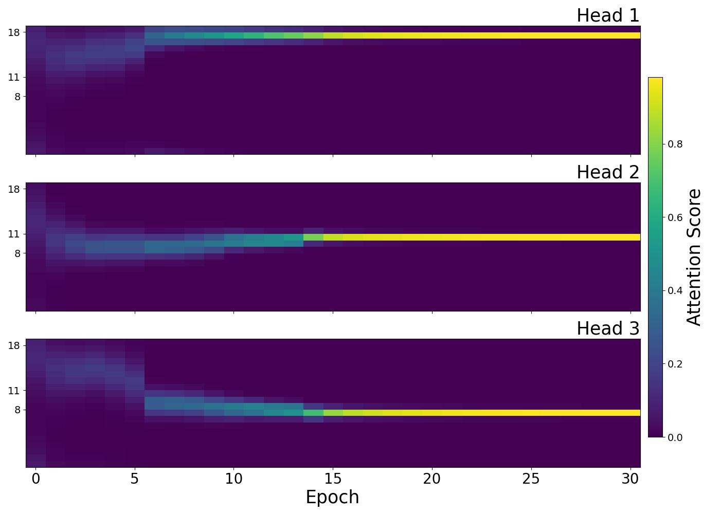
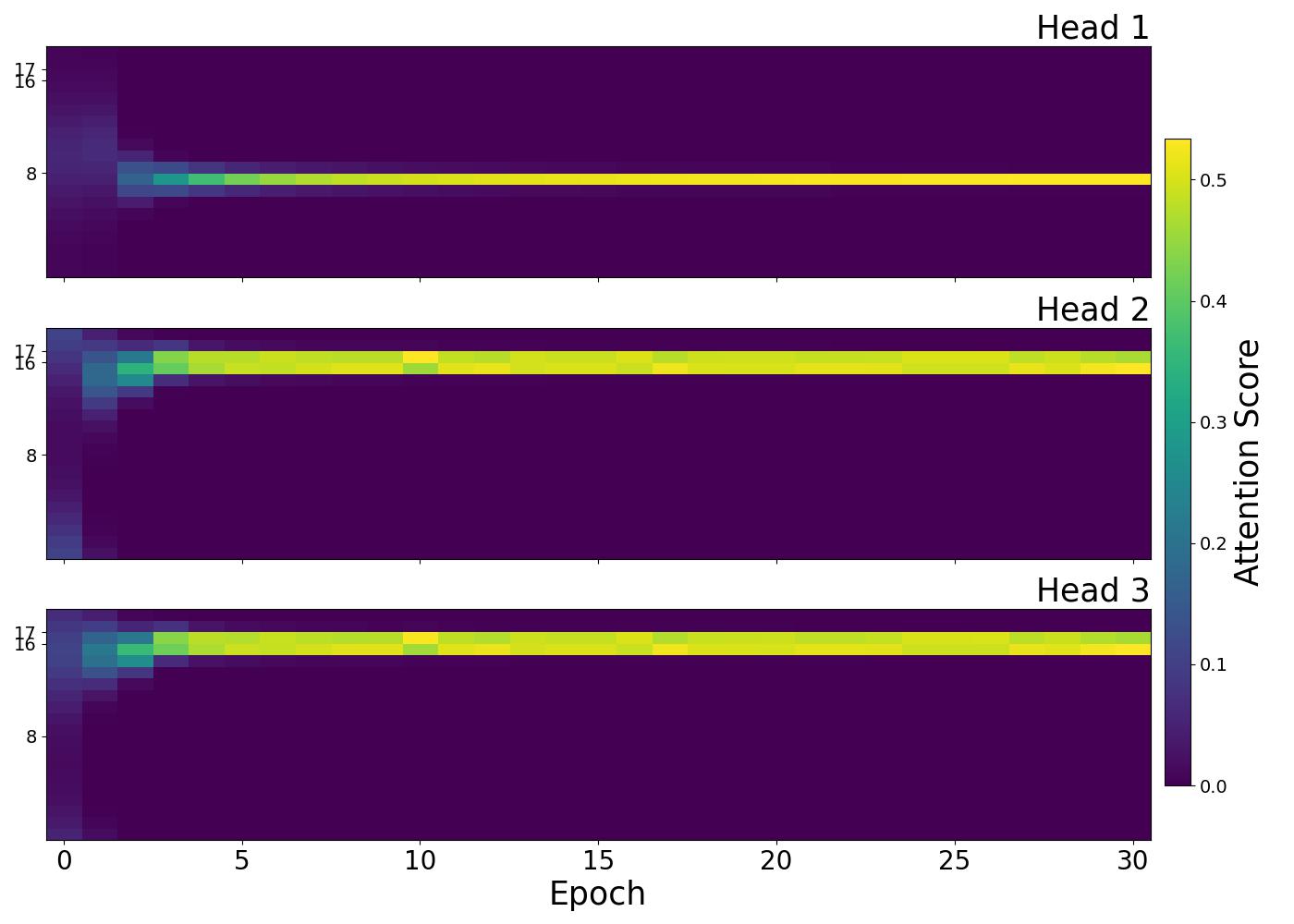
Figure 2: Two heat maps of soft attention training. When there are no neighboring bits each head attend to a separate bit with a score very close to 1 (sub-figure on the left). If there exist neighboring bits (sub-figure on the right), a pair of attention heads could learn the same direction, which is in the middle of the positional embeddings of the neighboring bits.

To demonstrate that attention heads converge to a hard attention solution unless there exist neighboring bits in the parity set, we conducted small-scale experiments with $n=20,k=3$, and trained the attention heads for 30 epochs. As illustrated in the left subfigure of Fig. 2, when the parity bits (e.g., positions $8$, $11$, and $18$) are non-adjacent, the three heads converge to focus exclusively on distinct bits, with each head allocating nearly all attention to a single position.

In contrast, the right subfigure highlights a different behavior when parity bits are neighbors, such as positions $16$ and $17$. Here, two heads often attend to the neighboring bits with nearly identical attention scores. The learned attention directions for these heads align with the middle point between the positional embeddings of the adjacent bits. For example, the attention weights for the second head $[a^{(2)}_{13},a^{(2)}_{14}]^{T}$ converge to the scaled vector $c\cdot[\sin(\frac{2\pi\cdot 16.5}{n}),\cos(\frac{2\pi\cdot 16.5}{n})]^{T}$, which interpolates between the embeddings of positions $16$ and $17$ with $c$ being a learned scaling factor. This phenomenon suggests that neighboring bits will cause overlapping attention learning, preventing attention heads from selecting positions independently, thus making inferencing using hard attention impossible under this circumstance.

References

- Ba et al. (2022) Jimmy Ba, Murat A. Erdogdu, Taiji Suzuki, Zhichao Wang, Denny Wu, and Greg Yang. High-dimensional asymptotics of feature learning: How one gradient step improves the representation. In Sanmi Koyejo, S. Mohamed, A. Agarwal, Danielle Belgrave, K. Cho, and A. Oh, editors, Advances in Neural Information Processing Systems 35: Annual Conference on Neural Information Processing Systems 2022, NeurIPS 2022, New Orleans, LA, USA, November 28 - December 9, 2022, 2022. URL http://papers.nips.cc/paper_files/paper/2022/hash/f7e7fabd73b3df96c54a320862afcb78-Abstract-Conference.html.
- Bergsträßer et al. (2024) Pascal Bergsträßer, Chris Köcher, Anthony Widjaja Lin, and Georg Zetzsche. The power of hard attention transformers on data sequences: A formal language theoretic perspective. CoRR, abs/2405.16166, 2024. doi: 10.48550/ARXIV.2405.16166. URL https://doi.org/10.48550/arXiv.2405.16166.
- Bhattamishra et al. (2023) Satwik Bhattamishra, Arkil Patel, Varun Kanade, and Phil Blunsom. Simplicity bias in transformers and their ability to learn sparse boolean functions. In Anna Rogers, Jordan L. Boyd-Graber, and Naoaki Okazaki, editors, Proceedings of the 61st Annual Meeting of the Association for Computational Linguistics (Volume 1: Long Papers), ACL 2023, Toronto, Canada, July 9-14, 2023, pages 5767–5791. Association for Computational Linguistics, 2023. doi: 10.18653/V1/2023.ACL-LONG.317. URL https://doi.org/10.18653/v1/2023.acl-long.317.
- Carion et al. (2020) Nicolas Carion, Francisco Massa, Gabriel Synnaeve, Nicolas Usunier, Alexander Kirillov, and Sergey Zagoruyko. End-to-end object detection with transformers. CoRR, abs/2005.12872, 2020. URL https://arxiv.org/abs/2005.12872.