Kolmogorov-Smirnov Estimation of Self-Similarity
in Long-Range Dependent Fractional Processes
Abstract
This paper investigates the estimation of the self-similarity parameter in fractional processes. We re-examine the Kolmogorov-Smirnov (KS) test as a distribution-based method for assessing self-similarity, emphasizing its robustness and independence from specific probability distributions. Despite these advantages, the KS test encounters significant challenges when applied to fractional processes, primarily due to intrinsic data dependencies that induce both intradependent and interdependent effects. To address these limitations, we propose a novel method based on random permutation theory, which effectively removes autocorrelations while preserving the self-similarity structure of the process. Simulation results validate the robustness of the proposed approach, demonstrating its effectiveness in providing reliable estimation in the presence of strong dependencies. These findings establish a statistically rigorous framework for self-similarity analysis in fractional processes, with potential applications across various scientific domains.
keywords:
Kolmogorov-Smirnov test, fractional Brownian motion , Self-similarity , Hurst exponent[inst1]organization=MEMOTEF, Sapienza University of Rome,Department and Organization country=Italy
1 Introduction
Many natural as well as artificial phenomena including turbulence, tree growth, gravitational waves or stock markets frequently exhibit complex patterns in which scaling or self-similarity emerges as a prominent characteristic [8, 25, 4]. In these fields, self-similarity refers to the repetition of patterns or structures, and it plays a crucial role in uncovering meaningful features for applications, including pattern recognition, fractal analysis, and image compression. Its relevance spans a wide range of applications, including telecommunication networks [24], hydrologic time series [33], and stock market prices [15, 18].
One of the parameters used to describe self-similarity in time series is the Hurst exponent . Introduced by Kolmogorov [26], it was related by Hurst to the phenomena of long memory [22, 23] and used by Mandelbrot and Van Ness to describe the non-markovian behaviour of the fractional Brownian motion (fBm), the unique mean-zero Gaussian process with stationary and self-similar increments [31]. FBm is the fractional extension of the standard Brownian motion: for the process is persistent and has long memory, while for the process exhibits antipersistence and is mean-reverting. Only when the fBm has independent increments and is a semi-martingale, falling into the standard Brownian motion [2].
The property of self-similarity relates to the equivalence of the process’s scaled distributions. Consequently, the Kolmogorov-Smirnov (KS) test [27, 34], which assesses whether two univariate probability distributions are indistinguishable [32], emerges as a natural choice to test whether a process exhibits self-similarity across different time scales. In contrast, the most popular estimators of the Hurst parameter—encompassing time-domain methods (e.g., R/S statistic [30], aggregated variance method [5], and Higuchi’s method [21]), frequency-domain methods (e.g., modified periodogram [20] and Whittle estimator [35]), and time-scale methods (e.g., Abry and Veitch’s wavelet-based approach [1] and the diffusion entropy method [19])—rely on specific moments of the data (usually mean, absolute moments or variance) rather than analyzing how the entire distribution scales. This makes their robustness questionable to some extent, since they appear to introduce non-linear biases into the estimation process [12, 13, 14, 3].
In 2004 a new distribution-based method was proposed to detect the self-similarity parameter [6]: the Hurst exponent is estimated as the value of that minimizes the KS statistic, evaluated with respect to the minimal and maximal elements of the space of rescaled probability distribution functions for a self-similar process. Being distribution-free, this method is robust with respect to infinite-moments self-similar stochastic processes. However, the KS statistic is designed for independent and identically distributed (i.i.d.) data. Consequently, significant challenges emerge when attempting to extend its application to dependent data:
-
•
Fractional Brownian motion (fBm) or other fractional processes exhibit dependence when the , which complicates the estimation of the self-similarity parameter. For , the presence of positive dependence among the data leads to an effective reduction in sample size, manifesting as an excessive rate of rejection of the null hypothesis for identical distributions (Type 1 error). Conversely, for , the negative dependence results in an effective increase in sample size, leading to an excessive acceptance of the null hypothesis (Type 2 error). This poses a significant challenge in determining the critical threshold that governs the significance of the KS statistic, as its behavior exhibits a non-linear dependence on the Hurst exponent . We term this issue the intradependent problem.
-
•
In estimating the self-similarity parameter, the KS test is performed between the rescaled probability distributions of the same starting sample. This fact introduces further dependence among the data when applying the KS test. In particular, it is observed from the results that the distribution of the KS statistic depends not only on due to the intradependent problem, but also on the scaling factor of the distribution of a self-similar process. We call this effect as interdependent problem.
The contribution of this paper is to overcome both the intradependent and interdependent problems by using random permutation theory to break the autocorrelation structure contained in fractional data without affecting their self-similarity structure. By circumventing the above problems, we provide a method which makes the KS statistic robust with respect to dependent data, even when the autocorrelation is very strong. Certainly, this is not the first attempt to make the KS statistic robust with respect to data dependence. To mitigate its influence, various strategies have been proposed in literature, but most of the solutions are either ad hoc or tailored to specific dependence models; as such, they are not entirely satisfactory. For example, [37] recommends a corrective approach for datasets generated by second-order auto-regressive processes with known parameters;
[16] examine the effects of first-order autocorrelation and conclude that dependence leads to a reduction in the count of effectively independent observations, even if this bias diminishes to negligible levels when the first-order autocorrelation is within the range of and as the sample size increases;
[10] introduce a methodology that incorporates all lagged bivariate copulas to capture non-linear temporal dependencies, while [29] evaluates three methodologies, determining that Monte Carlo simulations offer the most effective solution.
Investigating the impact of dependence on the critical values of the KS distribution is particularly relevant in the context of fBm. This is because the presence of long-term memory significantly influences the Effective Sample Size (ESS)111The ESS represents the equivalent number of independent observations in a dataset, accounting for autocorrelation. It adjusts for dependence, providing a more accurate measure of the dataset’s informational content as if the observations were independent., as positive dependence reduces the statistical power of tests. This occurs because dependent observations contain less information than independent ones. The ESS from observations with autocorrelation function is defined by [36] as
| (1) |
From (1), it is easy to see that the ESS can exceed the number of observations in the sample in presence of negative autocorrelation (), and this represents a critical vulnerability when applying the KS statistic to fractional processes. This occurs because successive observations provide more independent information compared to cases with or without positive autocorrelation. Several factors contribute to this phenomenon: (a) each observation introduces contrasting information relative to its predecessor, increasing the informational content per observation; (b) negative autocorrelation reduces estimator variance, akin to having a larger sample of independent observations; and (c) error terms offset each other more effectively than in purely random series, enhancing the statistical efficiency and reliability of parameter estimates.
Given these limitations, we propose a radically different approach based on disrupting the autocorrelation function without affecting the distributions being compared by the KS statistic.
The paper is organized as follows. In Section 2 we recall the method introduced in [7]. Section 3 discusses the limits of applying the KS test to fBm due to interdependent and intradependent problems. In Section 4 random permutations are introduced to modify the initial method and solve these problems. Section 5 describes the steps of the new methodology, while – through extensive simulations – Section 6 provides evidence that the new methodology effectively corrects the biases of the KS test in estimating the self-similarity parameter of dependent data. Finally, Section 7 concludes.
2 Preliminaries and problem statament
2.1 Preliminaries
This section will recall some basic definitions about the Hurst parameter estimation method introduced by [6].
Definition 2.1.
A nontrivial222The process is trivial if is a constant almost surely for avery . stochastic process , stochastically continuous333The process is stochastically continuous at time if for any at , is - with (-), if for any
| (2) |
in the sense of finite-dimensional distributions444The finite-dimensional distributions of the stochastic process refer to the joint distributions of for fixed but arbitrary . The two stochastic processes and , defined on probability spaces and respectively and sharing the same state space , are said to have the same finite-dimensional distributions if, for any integer and real numbers and , it is: .
Remark 2.1.
Remark 2.2.
If is nontrivial, stochastically continuous at and -, if and only if almost surely for every . If , then (see [17]). To exclude degenerate cases, in the following we will assume that .
Following the idea set forth in [6], it is possible to estimate the self-similarity exponent by testing the equality of the distributions in equation (2) (or equation (3)). To this aim, the Kolmogorov-Smirnov test can be used.
Given a compact timescale set , denote by the cumulative distribution function of , for any . The equality in distribution in equation (2), for a specific , can be written as:
| (4) |
Introducing the variable , equation (4) can be rewritten as
| (5) |
Denoting as the set of the distribution functions of and considering the distance function ´ induced by the sup-norm with respect to , the diameter of on the metric space is then defined as
| (6) |
In the case of stationary increments it is possible to rewrite equations (4), (5) and (6) respectively as
| (7) |
| (8) |
and
| (9) |
The following propositions were proved for (for proofs see [6]):
Proposition 2.1.
is - if and only if, for any , .
Proposition 2.2.
Let be -. Then is non-increasing for and non-decreasing for .
Proposition 2.3.
Let , x or x, be a sequence of timescale sets such that, denoted by and by , it is and for . Then, with respect to the sequence , is: non-decreasing, if , or zero, if .
2.2 Problem statement
The idea behind this approach is to estimate the self-similarity parameter by seeking the value of that minimizes the Kolmogorov-Smirnov statistic of any pair of rescaled distributions of . In fact, from Propositions (2.1) and (2.2), the diameter of a self-similar process has a unique zero-valued minimum with respect , with the corresponding abscissa precisely equal to . However, the zero-valued minimum is a merely theoretical concept, because from an empirical point of view one deals with a sample of length – the observed path of the process – from which one extracts two rescaled samples and , of length and respectively. Thus, the empirical diameter
| (10) |
is always larger than zero. Therefore, the estimated self-similarity parameter is
| (11) |
provided that in equation (10) can be considered negligible.
It happens that the diameter exactly corresponds to the Kolmogorov-Smirnov statistic , which tests the null hypothesis that the two independent empirical cumulative distributions and are identical. For large samples, the null hypothesis is rejected at the significance level if
| (12) |
An application of this method is illustrated in Figure 1: 1000 sample paths of Brownian motion, each of length , were generated. Two sets of increments, and , were then extracted, with and , respectively555In [6] it is proved that there is no loss of generality in setting .. Since Brownian motion is self-similar with , the diameter passes the Kolmogorov-Smirnov test at a level in the neighborhood of that value: .
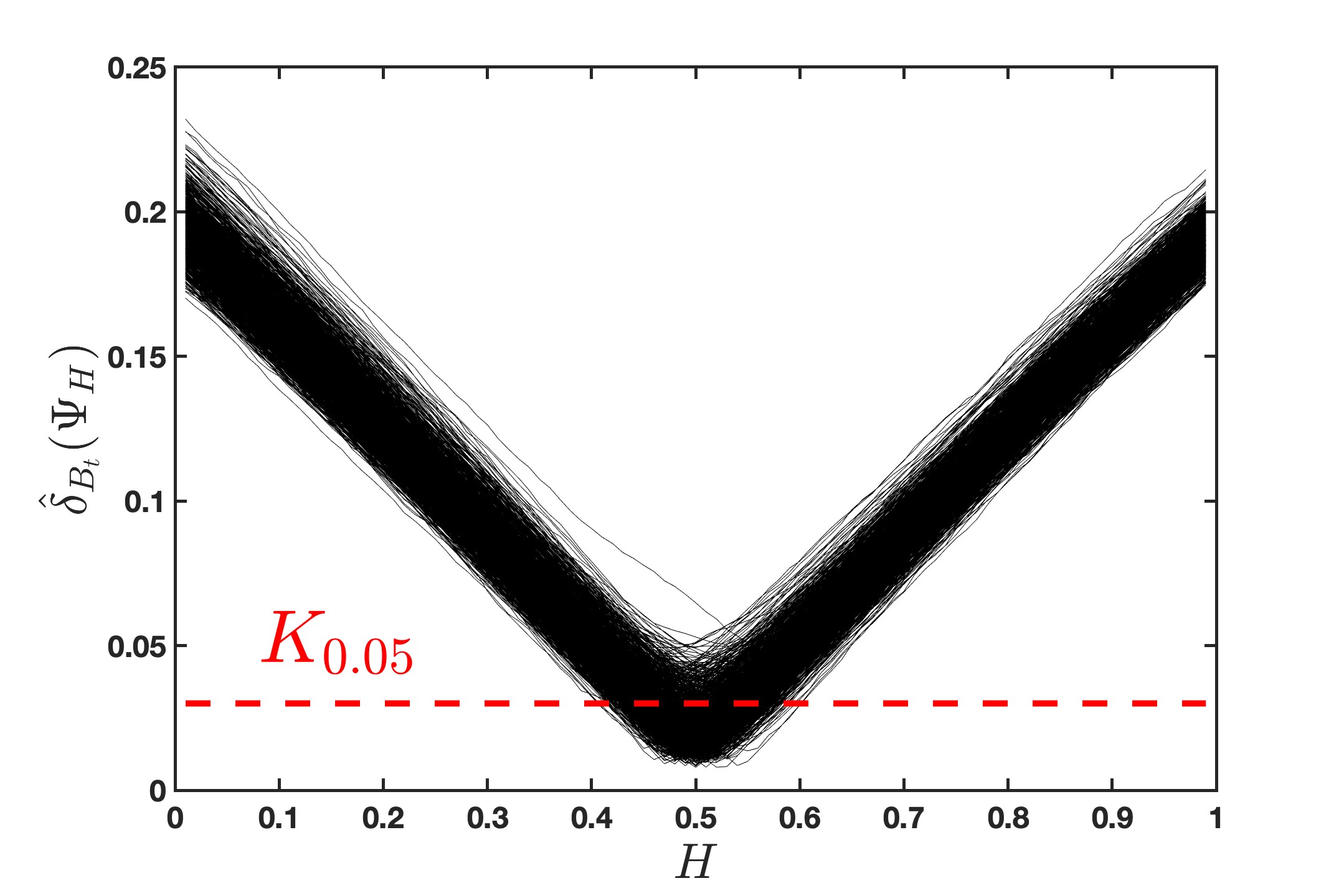
The main challenge in applying this method to estimate the self-similarity parameter of fractional processes lies in their inherent dependence, which causes the distribution of the test statistic to deviate from (12), since this covers only the case of independent samples. For dependent fractional processes, a bias arises, leading to either a Type 1 or Type 2 error depending on the value of (see Figure 2).
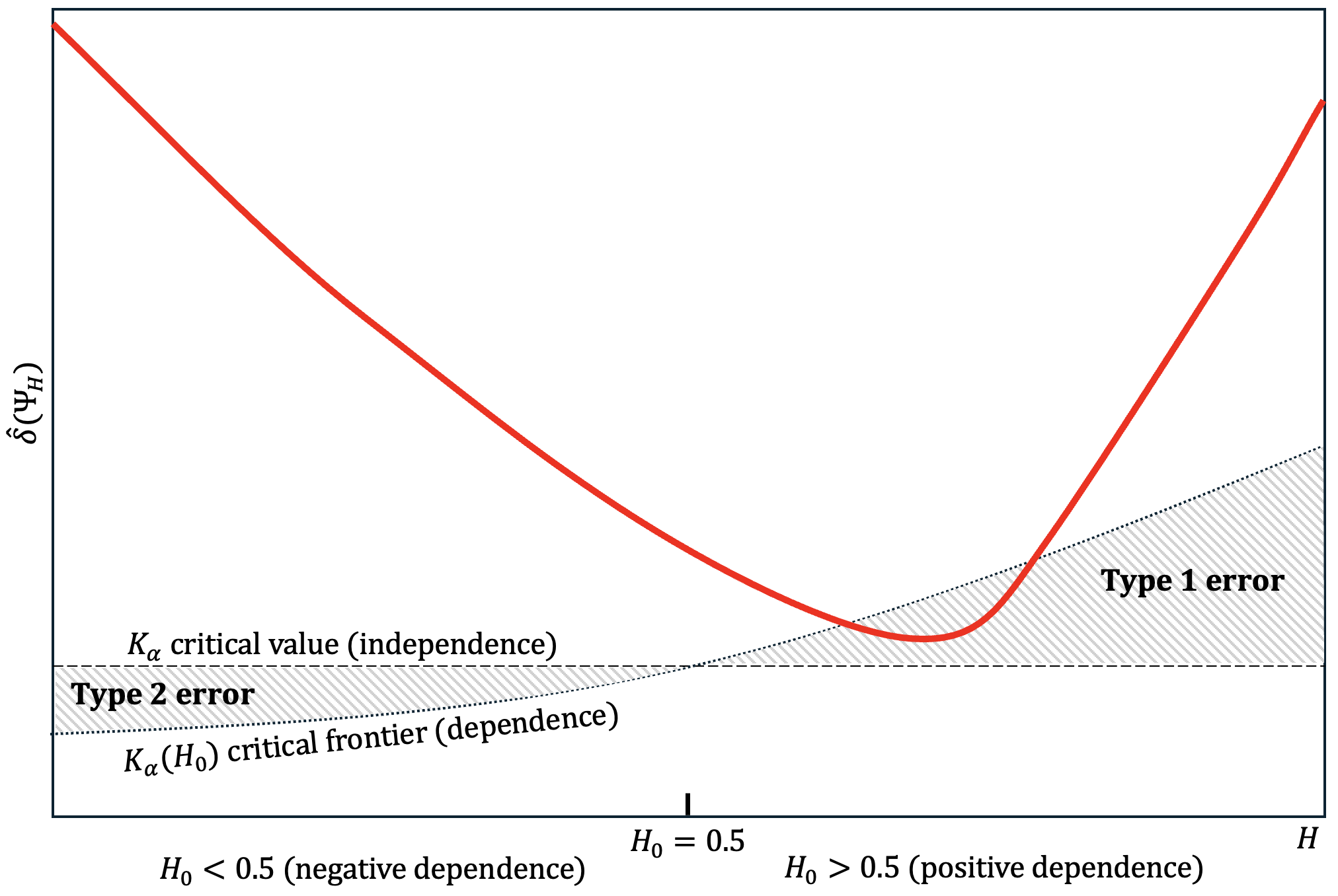
In general, when independence does not hold, the KS critical value tends to be too restrictive for moderate to high levels of positive autocorrelation and too lenient for moderate to high levels of negative autocorrelation. To mitigate the influence of dependence, various strategies have been proposed (as discussed in the Introduction, see e.g. [37, 16, 10, 29]), but none appears to be satisfactory with even highly dependent data, as is the case of fractional processes with far from 0.5.
3 KS distribution and fractional processes
The method outlined in the previous Section can be applied to any self-similar process, provided of course that a solution is found to eliminate Type 1 and Type 2 errors from the significance analysis of statistic (12). In the following, we will refer to the fractional Gaussian noise (fGn), the increment process of a fractional Brownian motion, as representative of the fractional (stationary) processes.
Focusing solely on the case of fGn does not lead to a loss of generality, as the decorrelation technique introduced in Section 4 to remove the correlation structure of data while preserving their distributional properties, is applicable to nearly all fractional processes. This is due to the fact that, among fractional processes, fractional Gaussian noise (fGn) typically exhibits the slowest decay in its autocorrelation function (ACF), particularly for , where the ACF follows a power-law decay of the form . As shown in Table 1, the autocorrelation functions of most fractional processes also decay as power laws, with a rate that is equal to or faster than that of fGn. Consequently, in the analysis presented in the subsequent sections, it suffices to focus on the fGn.
| Process | Asymptotic behaviour | Key Parameter |
|---|---|---|
| fGn | ||
| fPP | ||
| fLm | ||
| fOU | ||
| ARFIMA |
3.1 Fractional Brownian motion
For the reasons discussed in the previous paragraph, it is worthwhile to recall some properties of the fBm. A fractional Brownian motion (fBm) with Hurst exponent is a centered Gaussian, non-stationary and self-similar process defined as the following integral moving average representation [11] with respect to the Brownian motion
| (13) |
where is a scale parameter, , denotes the Gamma function and . From the covariance function
| (14) |
it is clear that the scaling parameter is introduced such that the variance at unit time is equal to . The peculiarity of the fBm is that, up to a multiplicative constant, it is the unique mean-zero Gaussian process with stationary and self-similar increments.
Regarding the stationarity of the increments , for any positive increment , we recall that and that the covariance function is independent of time:
| (15) |

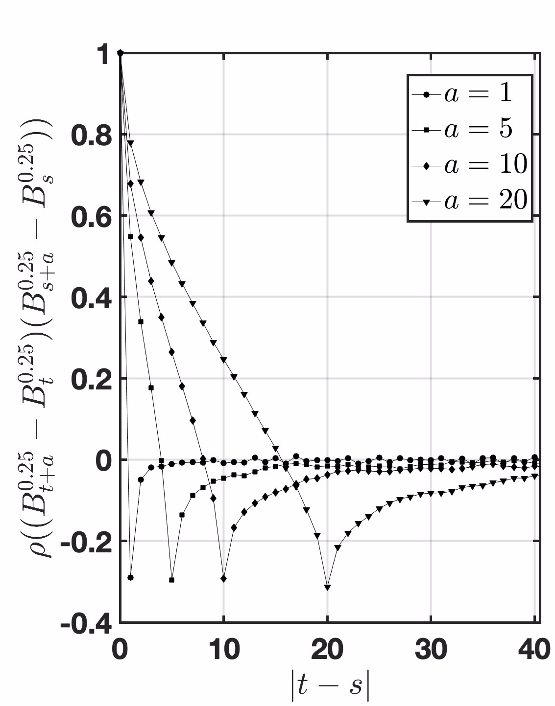

Therefore, as shown in Remark (2.1), the non-markovian behaviour of the fBm also affects the increment process, called fractional Gaussian noise (fGn). In Figure 3 it is represented the autocorrelation function which depends only on the temporal lag and the increments . Panel (a) illustrates the effect of the Hurst exponent on memory: for , the increments exhibit long memory, whereas for , they display short memory. In panel (c), corresponding to , we observe that the autocorrelation increases significantly as the increment grows, compared to the short-memory case shown in panel (b).
3.2 Analysis of the bias for the fGn
Applying equations (7)-(9) to an fBm with Hurst exponent , we have
| (16) |
Given a timescale set , with , the diameter becomes
| (17) |
In a computational analysis we simulate666The fractional Brownian motion was generated using the fbmwoodchan() MATLAB function, available in the FracLab Toolbox 2.02 (INRIA package), which is based on the Wood and Chan circulant matrix method [38]. Wood and Chan’s method simulates very accurate fGn, but this simulator returns fBm’s as a cumulative sum of fGn’s. As shown in [11], this approximation results in errors in the covariance structure of fBm’s generated as increases. For this reason the simulations in this paper will stop at the value of . By symmetry, the domain considered is . an fBm with . From the same process we extract two dependent increment samples and , with and respectively. Therefore, setting , the empirical diameter is
| (18) |
The estimated Hurst exponent is
| (19) |
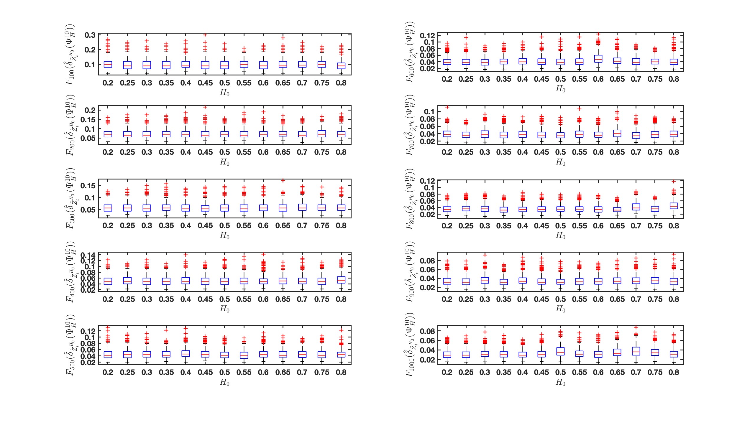
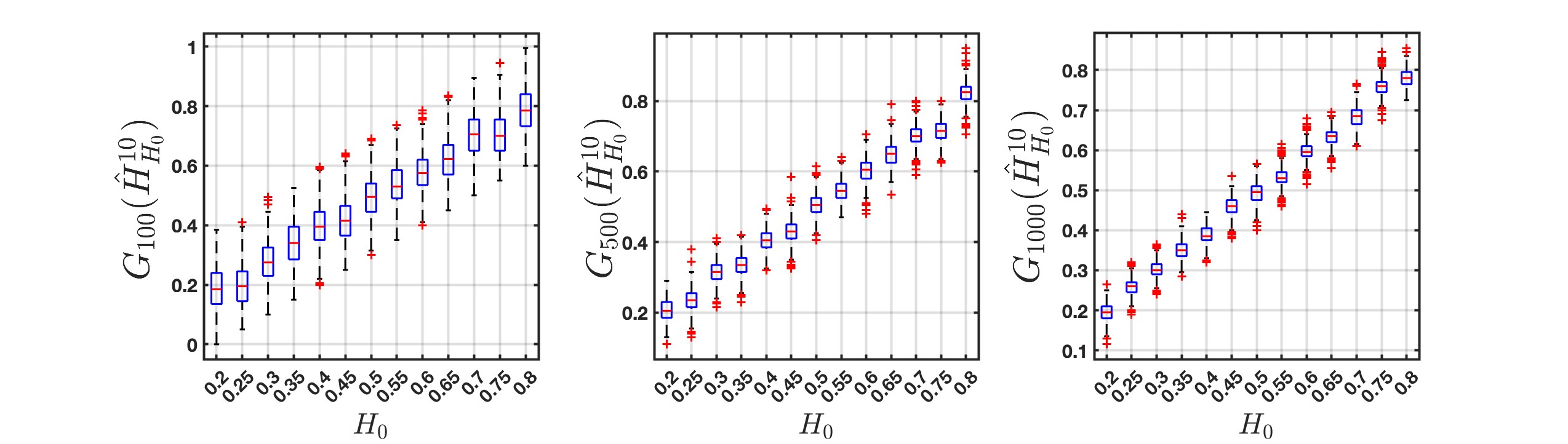
Given simulations with the same parameters , , and , we consider the distribution of the empirical minimum diameter and the distribution of the estimated Hurst exponent . In Figure 4, is shown for with . This experiment confirms the bias discussed in Figure 2 and shows that the distribution of the KS statistic increases as increases, precisely because the test is sensitive to autocorrelation: in the case of positive correlation (), the effective number of independent data points is artificially reduced, leading to an increase in the critical value . Conversely, when there is a negative correlation (), the effective number of independent data points is artificially inflated, resulting in a decrease in the critical value . We refer to this problem as the intradependent problem.

In Figure 5 we carried out two experiments, setting equal to 0.25 and 0.75, where we studied the distribution of the empirical diameters , and of the respective distributions of the estimated Hurst exponent , varying . According to the method outlined in Section 2, and in particular the results provided by Propositions (2.1), (2.2), and (2.3), the distribution of diameters should be independent of the chosen value of . However, in Figure 5, we observe that the distribution increases as grows. This discrepancy between theory and empirical results arises from the fact that the method involves extracting two rescaled series from the same original series, leading to a high correlation between the two series on which the KS test is applied. We refer to this issue as the interdependent problem.
4 Decorrelation by random permutation
The intradependent issue stems from the fact that the fGn exhibits the autocorrelation function given by (3.1), whose effects are illustrated in Figure 3. To overcome the intradependent problem, it is necessary to eliminate the dependence between increments and, consequently, disrupt the autocorrelation function of the fGn. To achieve this and to ease the understanding of the next proposition, it is useful to recall some fundamental concepts regarding the power spectrum and random permutation theory, since both tools will be used in the sequel.
Since the power spectrum of a stationary process is defined as the Fourier transform of its covariance function, one has that the autocovariance function can be obtained as the inverse Fourier transform of its power spectrum, i.e.
| (20) |
The power spectrum of the fractional Gaussian noise , for any , is defined as
| (21) |
with [11]. To disrupt the structure of (21), we need to introduce the random permutations of a sequence. Given the random sequence , we create a new sequence such that
| (22) |
where is a random permutation of the vector , uniformly distributed such that , with and the quotient and the remainder, respectively, of .
Based on Section 4 in [28], we can formulate the following
Proposition 4.1.
Let be a fractional Gaussian noise. Then, the new sequence , with an independent random phase uniformly distributed on the set of integers , has factorizable covariance in the limit of large permutation length
| (23) |
for .
Proof.
As in equation (22), under a random permutation , we can rewrite the fGn as the new sequence , whose covariance function is
| (24) |
Using the equality in distribution for any
| (25) |
In short, for any , we have
| (26) |
is not generally stationary, but it becomes stationary by adding an independent random phase uniformly distributed on the set of integers with probability . We obtain , such that , with covariance function
| (27) |
As shown in Appendix A of [28], is stationary and depends on both the initial power spectrum and the disorder of the random permutation . The spectral density is then defined by
| (28) |
Noting that i) , ii) uniformly in in any interval that does not contain , and iii) , we have
| (29) |
The proof is concluded noting that equation (29) is the covariance function of a white noise. ∎
Remark 4.1.
Given the stationarity of a fractional Gaussian noise, aside from a multiplicative parameter, we can state that is the power spectrum of its autocorrelation function.
Proposition 4.1 states that for sufficiently large values of , we may consider the new random sequence as white noise. The speed of convergence of to the power spectrum of a white noise depends on the regularity of the initial power spectrum . In [28] it is shown for NRZ and Biphase processes that their permuted sequences converge to a white noise for . For the fGn, we can repeat the same experiment done in Figure 3 starting from fBm with and . Applying the random permutation vector , with the permutation length equal to the entire length of the fGn, we compute the autocorrelation function of the permuted sequences . In Figure 6 the autocorrelation of is the same as a white noise, even for very small values of (see ). Therefore, this experiment suggests that for a random permuted fGn, the convergence of its power spectrum to that of a white noise is very fast.

Remark 4.2.
Random permutation acts only on the order of the elements of a sequence and not on their distribution. So the structure of self-similarity is maintained
The above technique removes the intradependence issue. To overcome also the interdependent problem, given a sampled fBm of length and considered the two associated fGns and of length and , respectively, we extract from them two random subsequences of length and use them to build the empirical cumulative distribution functions in (10). Thus, in addition to applying random permutation to eliminate the internal correlation of each sequence, we also eliminate the correlation between the two sequences while maintaining the self-similarity structure.
5 Computational pipeline
In the following, we summarize the steps of the novel method proposed in Section 4, which will be employed in the simulation study presented in Section 6.
-
1.
Set the Hurst exponent and simulate an fBm of length
-
2.
Set a compact set of timescales with and extract two fGns and
-
3.
Generate a temporal random permutation and from and the two subsequences and are extracted with length ;
-
4.
After selecting a dense set of values for testing self-similarity, the KS test is performed for each to compare and and the corresponding KS statistic is obtained
-
5.
The self-similarity parameter is estimated as
(30) -
6.
The statistic is compared with the critical values of the standard KS distribution. Clearly, the proximity between the theoretical and empirical significance levels is studied for . This assumption is necessary to isolate the issue of the variance of estimator (30) from the intrinsic variability of the distribution of the KS statistic.
6 Simulation study
In this section, we applied the method described in Section 5 to show that it solves both intradependent and interdependent problems, making the method introduced in 2004 more robust. In the next simulations, the length of fBm is set as . Any distribution is the result of simulations.
6.1 Intradependent problem
Step 1 in Section 5 was iterated for multiple values of with and setting .
We observe (Figure 7(a)) that the distributions remain stable – i.e. no noticeable shifting biases are present in the plots – with respect to , with subsequence lengths and . The corresponding distributions are plotted in Figure 7(b) as varies. As we should expect, as increases, the numerosity of the data also increases and therefore the estimate improves.
6.2 Interdependent problem
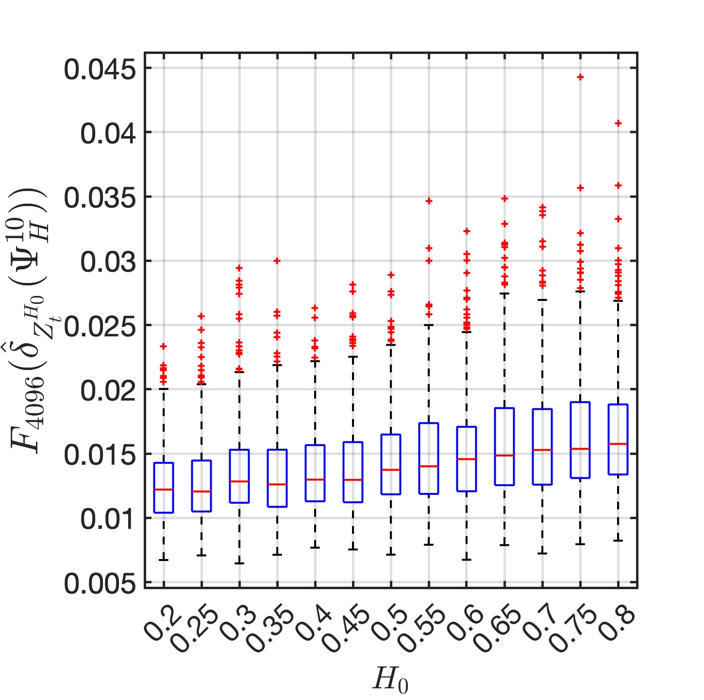
To show that the new method does not depend on the scaling factor, we iterated step 2 in section 5 for different values of and for (Figure 8(a)) and (Figure 8(c)). The estimates of are shown in Figure 8(b) and Figure 8(d), respectively.
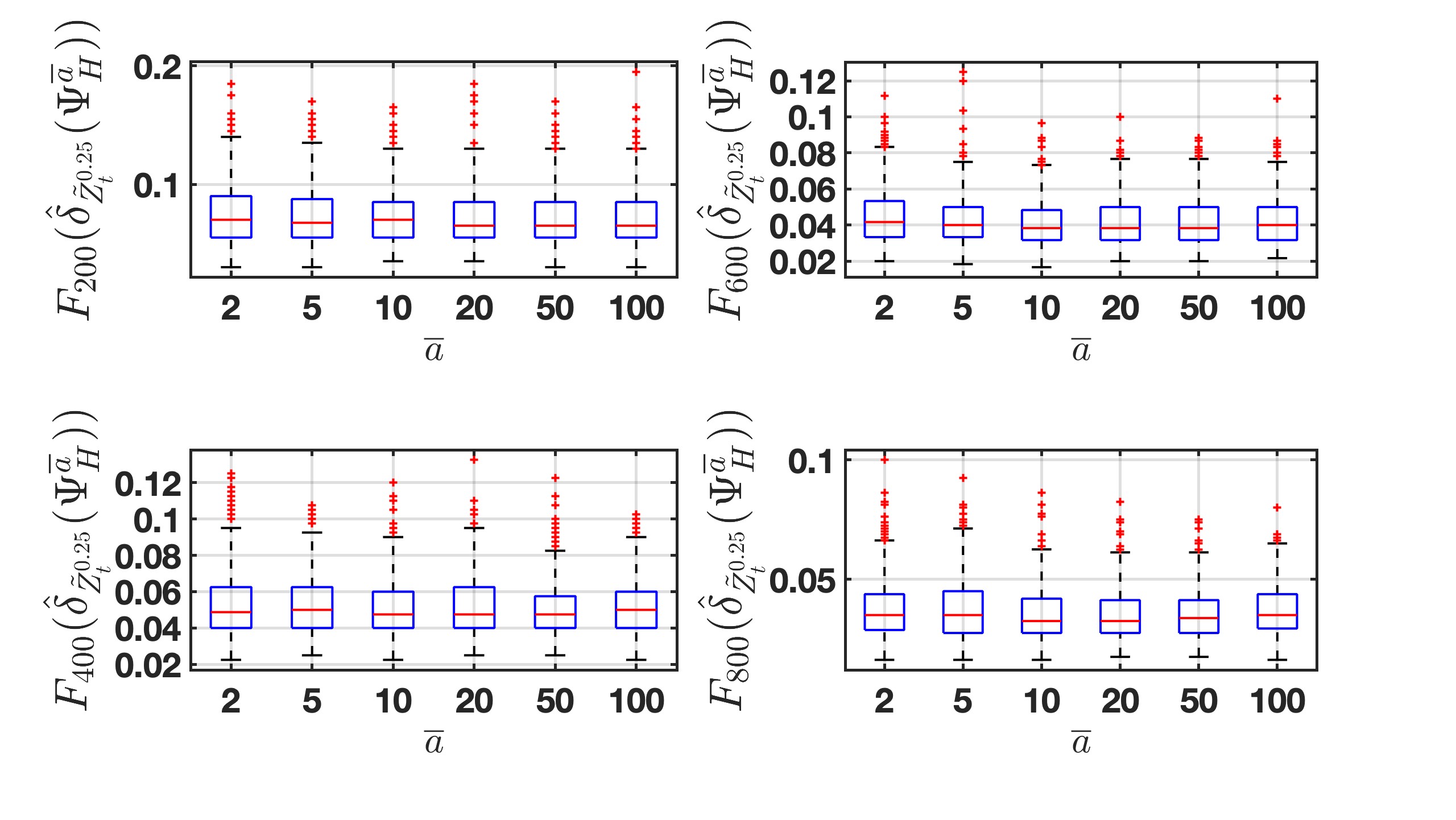
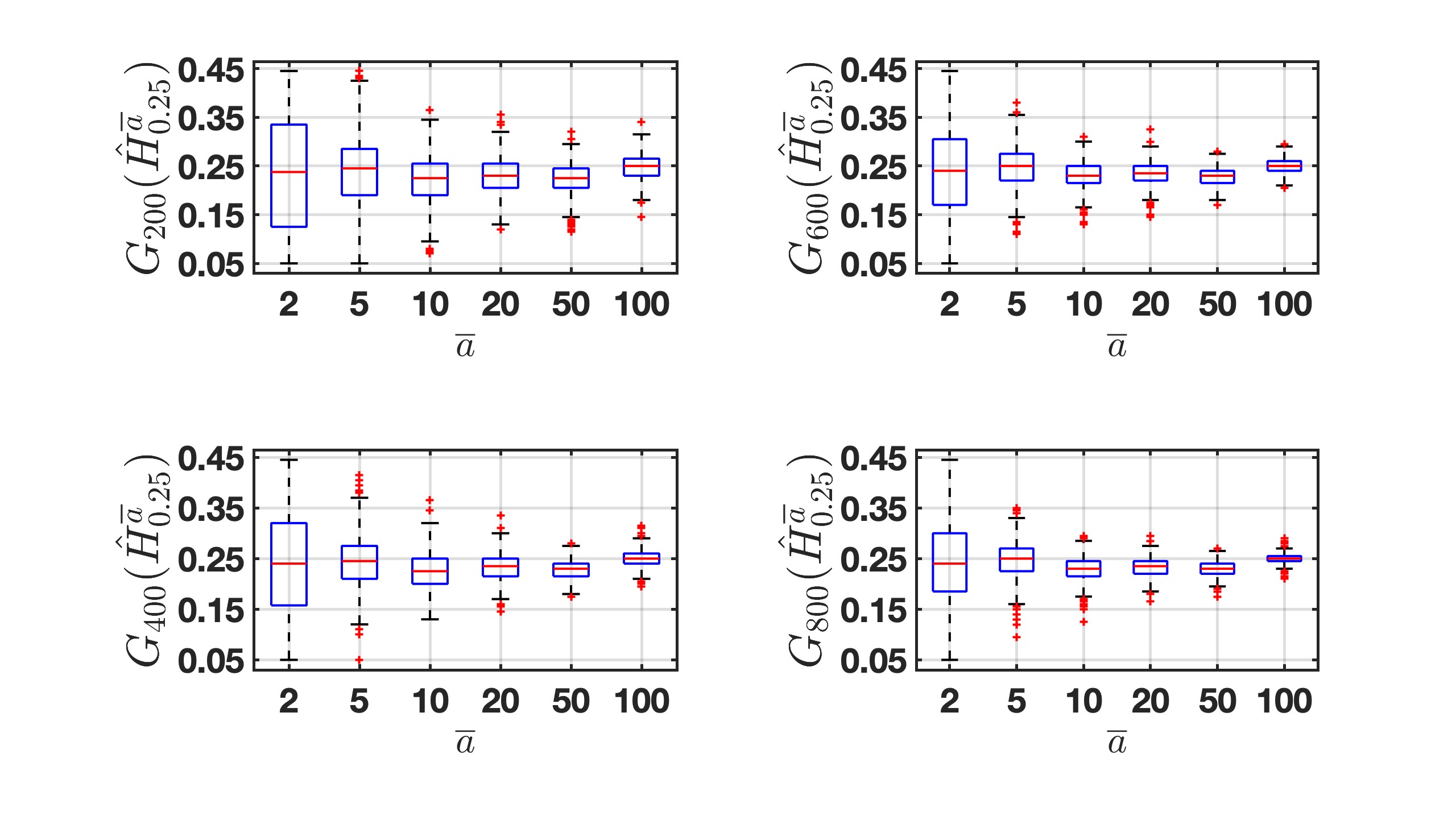
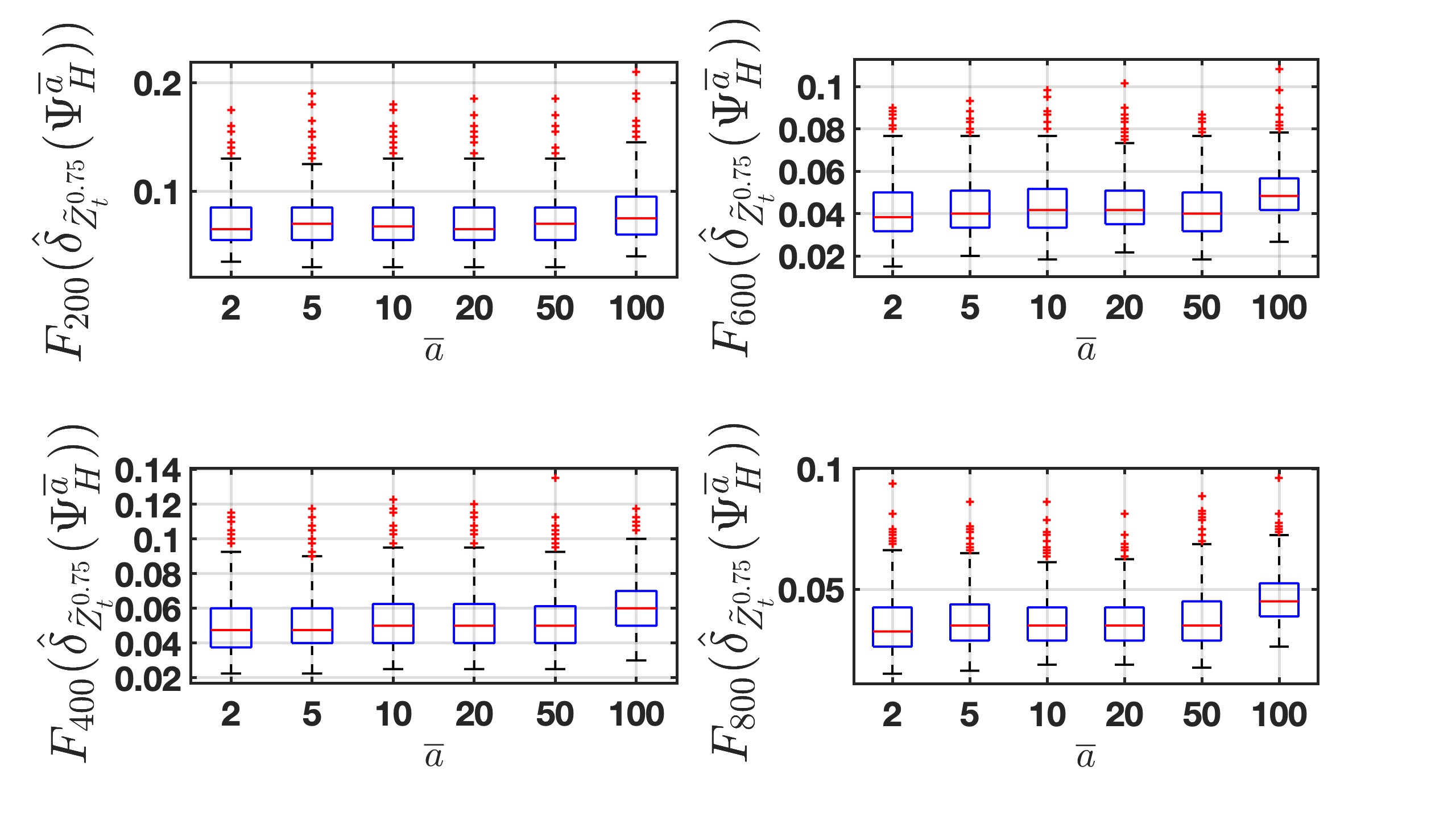
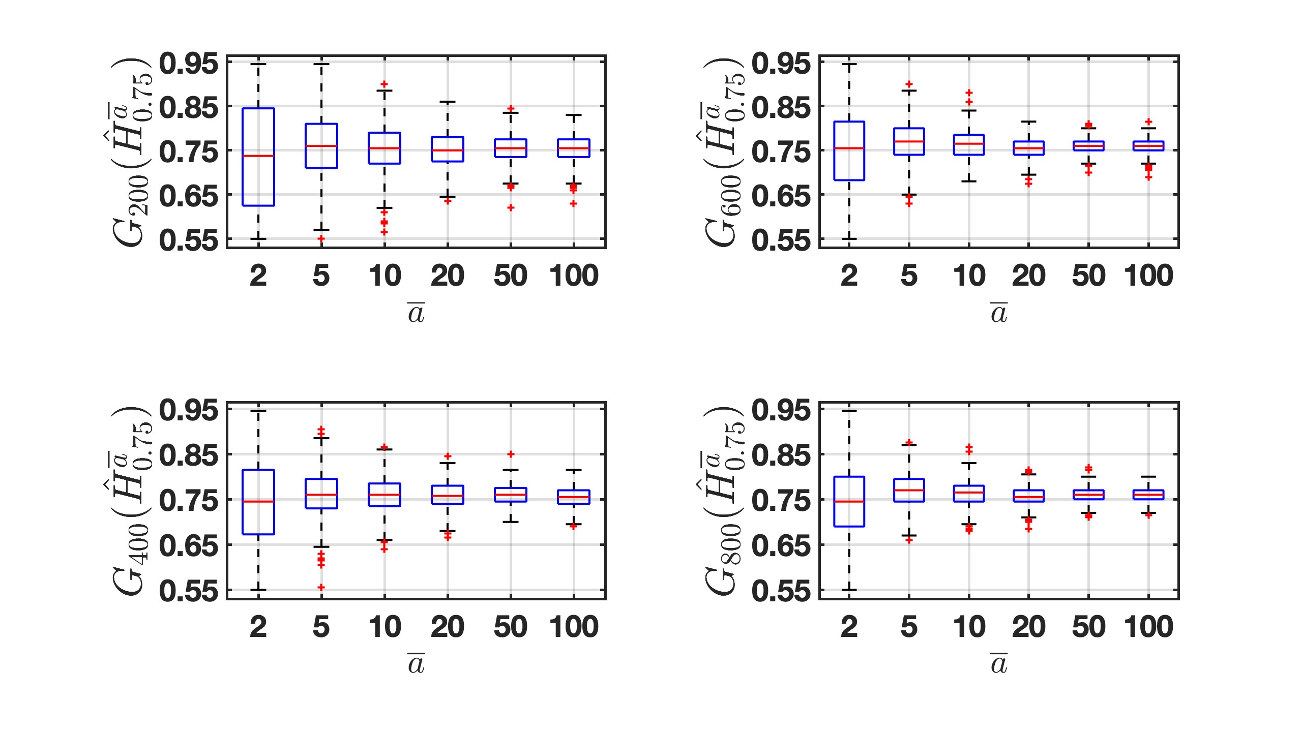
By comparing these simulations with those without randomization in Figure 5, we observe that the distributions exhibit greater stability, and the variances of the distributions decrease as the length of the subsequence increases. Furthermore, while no noticeable growth is observed in the distributions for , the opposite trend is evident for at high values of . Nonetheless, as shown in [9], the KS test remains effective even for sample sizes as small as . This ensures that the issue can be mitigated by maintaining low values of .
| 0.2 | 0.075 | 0.039 | 0.020 | 0.006 |
| 0.3 | 0.073 | 0.035 | 0.021 | 0.007 |
| 0.4 | 0.075 | 0.035 | 0.029 | 0.005 |
| 0.5 | 0.086 | 0.035 | 0.018 | 0.007 |
| 0.6 | 0.081 | 0.035 | 0.026 | 0.007 |
| 0.7 | 0.074 | 0.041 | 0.027 | 0.005 |
| 0.8 | 0.084 | 0.040 | 0.026 | 0.003 |
| 0.2 | 0.075 | 0.030 | 0.024 | 0.007 |
| 0.3 | 0.083 | 0.039 | 0.029 | 0.010 |
| 0.4 | 0.101 | 0.035 | 0.035 | 0.006 |
| 0.5 | 0.084 | 0.037 | 0.027 | 0.006 |
| 0.6 | 0.106 | 0.054 | 0.032 | 0.005 |
| 0.7 | 0.105 | 0.036 | 0.030 | 0.007 |
| 0.8 | 0.107 | 0.046 | 0.022 | 0.007 |
| 0.2 | 0.099 | 0.040 | 0.032 | 0.006 |
| 0.3 | 0.075 | 0.040 | 0.027 | 0.006 |
| 0.4 | 0.077 | 0.047 | 0.034 | 0.013 |
| 0.5 | 0.099 | 0.036 | 0.033 | 0.012 |
| 0.6 | 0.111 | 0.063 | 0.042 | 0.007 |
| 0.7 | 0.101 | 0.040 | 0.025 | 0.013 |
| 0.8 | 0.121 | 0.053 | 0.042 | 0.007 |
7 Conclusion
This study revisits the Kolmogorov-Smirnov (KS) test applied to estimate the self-similarity parameter in fractional processes, highlighting its limitations in handling data dependencies. The inherent intradependencies and interdependencies within fractional processes undermine the reliability of traditional KS-based approaches.
To overcome these challenges, we proposed a random permutation-based method that effectively disrupts the autocorrelation structure of fractional Gaussian noise while preserving the self-similarity property of the process. The slow decay of the autocorrelation function of fGn ensures that the method can be effectively applied to other fractional processes, whose autocorrelation functions decay at least as fast as, if not faster than, that of the fGn. Simulation results validate the robustness of the proposed approach, exhibiting consistent performance across a range of Hurst exponent values and scaling factors.
By enhancing the applicability of distribution-based self-similarity estimation, this method provides a reliable framework for analyzing fractional processes in diverse fields such as turbulence, finance, and telecommunications. Future research directions include extending this methodology to multidimensional or non-Gaussian processes, further broadening its scope and applicability.
Declaration of generative AI in scientific writing During the preparation of this work, the authors used ChatGPT in order to improve the readability and language of the manuscript. After using this tool/service, the authors reviewed and edited the content as needed and take full responsibility for the content of the published article.
References
- [1] P. Abry and D. Veitch. Wavelet analysis of long-range-dependent traffic. IEEE Transactions on Information Theory, 44(1):2–15, 1998.
- [2] S. Achard and J.-F. Coeurjolly. Discrete variations of the fractional Brownian motion in the presence of outliers and an additive noise. Statistics Surveys, 4:117–147, 2010.
- [3] D. Angelini and S. Bianchi. Nonlinear biases in the roughness of a fractional stochastic regularity model. Chaos, Solitons & Fractals, 172:113550, 2023.
- [4] T.W. Baumgarte, C. Gundlach, and D. Hilditch. Critical phenomena in the collapse of quadrupolar and hexadecapolar gravitational waves. Physical Review D, 107(8):084012, 2023.
- [5] J. Beran. Statistics for Long Memory Processes. Chapman and Hall, London, 1994.
- [6] S. Bianchi. A new distribution-based test of self-similarity. Fractals, 12(03):331–346, 2004.
- [7] S. Bianchi. A cautionary note on the detection of multifractal scaling in finance and economics. Applied Economics Letters, 12(12):775–780, 2005.
- [8] G. Cafiero and J.C. Vassilicos. Non-equilibrium turbulence scalings and self-similarity in turbulent planar jets. Proceedings of the Royal Society A, 475(2225):20190038, 2019.
- [9] I.M. Chakravarti, R.G. Laha, and J. Roy. Handbook of methods of applied statistics. Wiley Series in Probability and Mathematical Statistics (USA) eng, 1967.
- [10] R. Chicheportiche and J-P. Bouchaud. Goodness-of-fit tests with dependent observations. J. Stat. Mech.: Theory and Experiments, 11:P09003, 2011.
- [11] J.-F. Coeurjolly. Simulation and identification of the fractional Brownian motion: a bibliographical and comparative study. Journal of Statistical Software, 5:1–53, 2000.
- [12] R. Cont and P. Das. Quadratic variation along refining partitions: constructions and examples. J. Math. Anal. Appl., 512(2):126173, 2022.
- [13] R. Cont and P. Das. Quadratic variation and quadratic roughness. Bernoulli, 29(1):496–522, 2023.
- [14] R. Cont and P. Das. Rough volatility: fact or artefact? Sankhya B, pages 1–33, 2024.
- [15] R. Cont, M. Potters, and J.-P. Bouchaud. Scaling in stock market data: Stable laws and beyond. In B. Dubrulle, F. Graner, and D. Sornette, editors, Scale Invariance and Beyond, pages 75–85, Berlin, Heidelberg, 1997. Springer Berlin Heidelberg.
- [16] P. Durilleul and P. Legendre. Lack of robustness in two tests of normality against autocorrelation in sample data. Journal of Statistical Computation and Simulation, 42(1-2):79–91, 1992.
- [17] P. Embrechts and M. Maejima. Selfsimilar Processes. Princeton University Press, 2002.
- [18] M. Garcin. Forecasting with fractional Brownian motion: a financial perspective. Quantitative Finance, 22(8):1495–1512, 2022.
- [19] P. Grigolini, L. Palatella, and G. Raffaelli. Asymmetric anomalous diffusion: an efficient way to detect memory in time series. Fractals, 9(04):439–449, 2001.
- [20] U Hassler. Regression of spectral estimators with fractionally integrated time series. Journal of Time Series Analysis, 14(4):369–380, 1993.
- [21] T. Higuchi. Approach to an irregular time series on the basis of the fractal theory. Physica D, 31:277–283, 1988.
- [22] H.E. Hurst. Long-term storage capacity of reservoirs. Transactions of the American Society of Civil Engineers, 116(1):770–799, 1951.
- [23] H.E. Hurst, R.P. Black, and Y.M. Simaika. Long-term storage. An experimental study. London, 1965.
- [24] H.-D. J. Jeong. Modelling of self-similar teletraffic for simulation. PhD thesis, University of Canterbury, 2002.
- [25] T. Kalliokoski, R. Sievänen, and P. Nygren. Tree roots as self-similar branching structures: axis differentiation and segment tapering in coarse roots of three boreal forest tree species. Trees, 24:219–236, 2010.
- [26] A.N. Kolmogorov. Wienershe spiralen und einige andere interessante kurven im hilbertishen raum. DAS of the URSS (Nat. Sciences), 26:115–118, 1940.
- [27] A.N. Kolmogorov. Foundations of the theory of probability, 1950.
- [28] B. Lacaze and D. Roviras. Effect of random permutations applied to random sequences and related applications. Signal Processing, 82(6):821–831, 2002.
- [29] J.R. Lanzante. Testing for differences between two distributions in the presence of serial correlation using the kolmogorov–smirnov and kuiper’s tests. International Journal of Climatology, 41(14):6314–6323, 2021.
- [30] B.B. Mandelbrot and M.S. Taqqu. Robust R/S analysis of long run serial correlation. Bulletin of the International Statistical Institute, 48(2):69–104, 1979.
- [31] B.B. Mandelbrot and J.W. Van Ness. Fractional Brownian motions, fractional noises and applications. SIAM Review, 10(4):422–437, 1968.
- [32] R. A. Olea and V. Pawlowsky-Glahn. Kolmogorov–Smirnov test for spatially correlated data. Stochastic Environmental Research and Risk Assessment, 23:749–757, 2009.
- [33] A.R. Rao and D. Bhattacharya. Comparison of Hurst exponent estimates in hydrometeorological time series. J. Hydrol. Eng., 4(3):225–231, 1999.
- [34] N.V. Smirnov. On the estimation of the discrepancy between empirical curves of distribution for two independent samples. Bulletin Mathematics University Moscou, 2(2):3–14, 1939.
- [35] M S Taqqu and V Teverovsky. On estimating the intensity of long-range dependence in finite and infinite variance time series. A Practical Guide to Heavy Tails: Statistical Techniques and Applications, 177:218, 1998.
- [36] H.J. Thièbaux and F.W. Zwiers. The interpretation and estimation of effective sample size. Journal of Climate and Applied Meteorology, 23(5):800–811, 1984.
- [37] M.S. Weiss. Modification of the kolmogorov-smirnov statistic for use with correlated data. Journal of the American Statistical Association, 73(364):872–875, 1978.
- [38] A.T.A. Wood and G. Chan. Simulation of stationary gaussian processes in [0, 1] d. Journal of Computational and Graphical Statistics, 3(4):409–432, 1994.