Force-free kinetic inference of entropy production
Abstract
Estimating entropy production, which quantifies irreversibility and energy dissipation, remains a significant challenge despite its central role in nonequilibrium physics. We propose a novel method for estimating the mean entropy production rate that relies solely on position traces, bypassing the need for flux or microscopic force measurements. Starting from a recently introduced variance sum rule, we express in terms of measurable steady-state correlation functions which we link to previously studied kinetic quantities, known as traffic and inflow rate. Under realistic constraints of limited access to dynamical degrees of freedom, we derive efficient bounds on by leveraging the information contained in the system’s traffic, enabling partial but meaningful estimates of . We benchmark our results across several orders of magnitude in using two models: a linear stochastic system and a nonlinear model for spontaneous hair-bundle oscillations. Our approach offers a practical and versatile framework for investigating entropy production in nonequilibrium systems.
Stochastic modeling is essential for describing complex phenomena characterized by randomness and fluctuations. Their breaking of time-reversal symmetry and energy dissipation are quantified by the entropy production [1, 2, 3, 4, 5, 6]. The irreversibility of stochastic traces can be directly used to infer the entropy production rate in a nonequilibrium steady state (NESS) [7, 8, 9, 10]. However, estimating exploiting violations of time-reversal symmetry typically requires observing stochastic trajectories whose length scales exponentially with , posing practical limitations. Recent advances offer an alternative approach by bounding entropy production using information-theoretic methods, leading to the development of thermodynamic uncertainty relations (TURs) [11, 12, 13, 14, 15, 16, 17, 18, 19, 20, 21, 22, 23, 24, 25]. Alternative methods require perturbation experiments to exploit the violation of the fluctuation-dissipation theorem [26, 27] by directly applying the Harada-Sasa relation [28]. Another possibility could be to directly measure microscopic forces or probability fluxes and use their relation with dissipation [29, 30], but this is challenging in most cases. Moreover, in many realistic scenarios, the system under study can only be partially observed, which further complicates the inference process. For discrete systems, this typically corresponds to observing coarse-grained or lumped mesostates, which aggregate numerous microstates whose individual transitions remain unobservable [31, 32, 33, 34, 35, 36, 37, 38, 39, 40, 41]. For continuous processes, limited information may result from spatial coarse-graining [42, 43, 44, 45] or from the partial observation of a subset of the Markovian degrees of freedom [46, 47, 48, 49]. While central to understanding irreversible processes, estimating entropy production remains a challenging and active area of ongoing research.
In this Letter, we introduce a novel framework for estimating directly from stochastic trajectories, without the need for additional force measurements or the challenging task of inferring irreversibility from trajectory data, and naturally extending to partially observed systems. In particular, we focus on the steady state dynamics of multiple degrees of freedom (DOFs) determined by the overdamped Langevin equations
| (1) |
with potentially non-conservative forces and white noise with mean and covariance . The system may be in contact with different thermal baths encoded in a diagonal temperature matrix . The mobility matrix is related to the diffusion matrix by the Einstein relation . According to stochastic energetics [29], in a NESS corresponds to the amount of heat dissipated in the environment per unit time,
| (2) |
where is the average heat injected into the heat bath at temperature and denotes the Stratonovich product. This formula often exposes two main empirical problems: (i) it requires measuring the forces acting on the relevant DOFs (which is challenging in most cases), and (ii) it often clashes with the impossibility of observing all relevant DOFs.
In [50, 51] we derived a formula for starting from the variance sum rule (VSR) involving the second derivative of the position correlation function and the covariances of microscopic forces. Expressed in terms of correlation functions and following Einstein’s summation convention, it takes the form:
| (3) |
where is the connected correlation matrix for the observable and is its second derivative evaluated at zero. Eq. (3) shows that the curvatures of the position correlation functions at short times are highly informative about dissipation. Still, the difficulties in estimating mobility and forces in experiments hinder the direct application of this formula. For example, in [50], we analyzed experimental measurements of red blood cell flickering [50], where only a single degree of freedom was observable and direct measurements of cellular forces were not accessible. To overcome these limitations, a reduced form of the VSR was employed to fit the experimental data, and, similar to [48, 52], modeling was necessary to compensate for the lack of information about the underlying system.
Starting from the VSR, we derive a new formula for (see (5) below) that does not rely on the evaluation of forces. First, we deal with cases where all relevant DOFs are visible, even if forces are not directly measurable. When some DOFs are not detectable, we derive bounds on , enabling a partial yet informative estimation process, provided that the mobility matrix is diagonal, as in the absence of hydrodynamic interactions. Rather than relying on real microscopic forces, our method focuses on estimating effective forces derived from the experimentally accessible probability density function (PDF) . In a NESS, the effective potential is given by and its gradient , scaled by , acts as an effective force. Beyond stochastic thermodynamics, the gradient of the log-probability, commonly referred to as the score function in statistical inference and machine learning, serves as the foundation for score matching methods [53]. These methods play a pivotal role in optimization and modeling frameworks such as energy-based models [54] and generative diffusion models [55, 56, 57, 58]. Additionally, score functions enable entropy production estimation within deep learning frameworks [59]. In our setting, we reformulate (3) in terms of effective forces using the definition of the mean local velocity , stemming from the Fokker-Planck equation associated with the Langevin equations (1),
| (4) |
which connects the real forces to . In this way, as shown in Section S1 of [60], we derive a new formula for from the VSR
| (5) |
where all terms can be directly inferred from position traces. Indeed, the diffusion matrix, , can be directly extracted from the position correlation matrix, , via
| (6) |
where denotes the symmetrized matrix and (see Section S4 in [60]). The second term on the right-hand side of Eq. (5) corresponds to the inflow rate
| (7) |
a time-symmetric quantity obeying fluctuation relations [61] and recently used to study the information content of stochastic traces [62]. can be determined from effective force measurements, which involves estimating using a kernel density estimator and computing the gradient with standard numerical tools, see Section S9 in [60] for more details. The connection between and was first established in [63], with the traffic , a key kinetic quantity also commonly referred to as dynamical activity or frenesy [64, 65, 66], providing the link between the two. This relationship is given by
| (8) |
and, together with (5), leads to the identification
| (9) |
The traffic represents the symmetric component of the stochastic action associated with the Langevin process. While its original definition [63] (see Eq. S16 in [60]) is based on microscopic forces, the new formulation (9) enables direct estimation from position measurements. To summarize, since both and can be expressed in terms of derivatives of position correlation functions and effective force covariances , both terms in (8) can be accurately evaluated from position traces. In the following examples, we will show that, typically, the traffic captures the behavior of better than . This may be due to the static nature of , which depends only on the steady-state PDF and may be insensitive to variations in dissipation, whereas is inherently dynamical. As the time-symmetric component of the stochastic action, it encodes details of the system kinetics that alone might not capture, suggesting that could serve as a more sensitive probe of non-equilibrium behavior.
To illustrate these ideas, we apply our method to two paradigmatic systems: (i) a two-dimensional linear system driven out of equilibrium by nonreciprocal forces and heat baths at different temperatures, and (ii) a nonlinear model describing spontaneous hair-bundle oscillations in bullfrog ears [67]. The linear system allows full analytical characterization and serves as a benchmark for testing the method, while the hair-cell model demonstrates the practical and biological relevance of the approach. Furthermore, we explore regions of the parameter space where varies substantially and show that this variability is predominantly captured and encoded by . This observation is particularly valuable since, in partial measurements, cannot be directly inferred, whereas partial measurements of still enable effective thermodynamic inference.
As a first example [68, 69, 70, 71, 72, 73], we consider a linear stochastic system where two DOFs and evolve according to the following coupled SDEs,
| (10) |
where , for simplicity. The stability conditions to ensure the existence of a NESS are and . can be calculated analytically (see Section S5 in [60]) and equals
| (11) |
From (11), one sees that and are strictly related to dissipation. When these parameters are different, the mechanical forces and heat fluxes are not balanced and probability currents are generated. The magnitude of these currents is proportional to , and is modulated by the kinetic term , which also sets the timescale of the system. Crucially, this kinetic term turns out to be exactly equal to the inflow rate, , which is independent of the dissipative parameters and . This fact suggests that the relevant information on the variability of is encoded primarily in . More detailed calculations related to (10) are provided in Section S5 in [60].
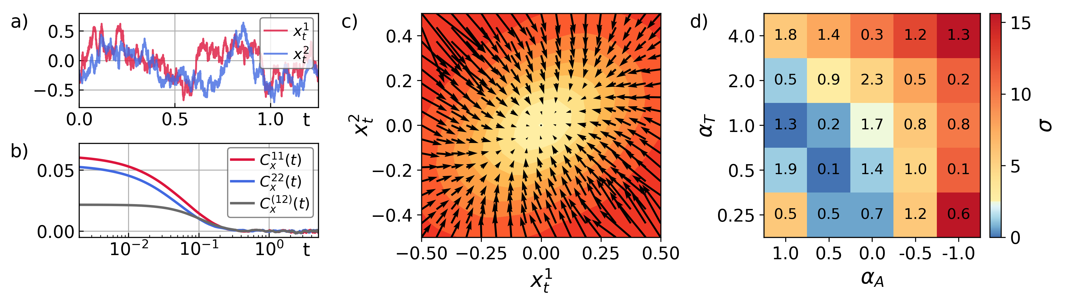
To test the predictive power of Eq. (5), we simulated 25 stochastic traces (Fig. 1a) with fixed inflow rate , and different dissipative parameters and . From these, we derived correlation functions (Fig. 1b) as well as and the effective forces (Fig. 1c). Technical details on how these elements have been processed to predict can be found in Section S9 in [60]. For each estimate we assess the quality of the prediction by evaluating the accuracy coefficient that quantifies how far, in units of the statistical error , the estimate is from the true value . The latter is evaluated from the analytical expression (11). Fig. 1d shows the accuracy obtained for all simulated traces, while is shown in the underlying heatmap. The inference process gives very good results with an average accuracy and for all simulated traces.
As a second example, we examine a nonlinear model of spontaneous hair-bundle oscillations in bullfrog ears [67], where the estimation of from experimental traces remains an active area of research [48, 52]. The model describes the interplay between mechanosensitive ion channels, molecular motor activity, and calcium feedback, capturing the system’s dynamics through two degrees of freedom: the position of the bundle and the center of mass of the molecular motors [74, 75, 76]. The system’s evolution follows:
| (12) |
where the potential describes the mechanical interactions within the system, including elastic forces and the gating dynamics of mechanosensitive ion channels, with its explicit form provided in Section S8 of [60]. Nonequilibrium driving arises from molecular motor activity, encoded in the effective temperature and the non-conservative force:
| (13) |
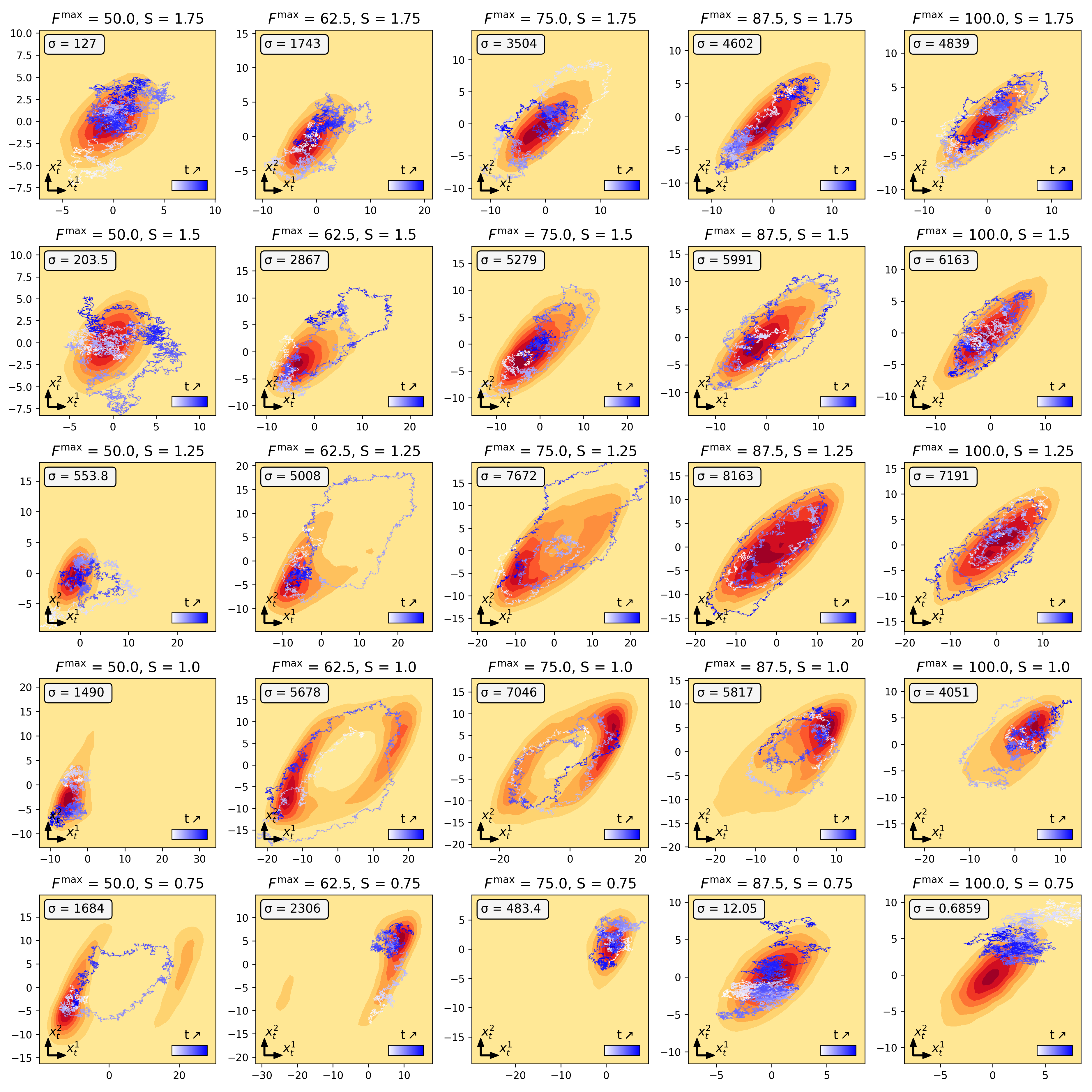
Here, is the maximum motor force, controls the strength of calcium-mediated feedback, and represents the probability of ion channel opening [77]. More details are provided in Section S8 in [60]. While characterizes enhanced fluctuations due to active processes, the main contributors to entropy production are the activity parameters and . Following the approach in [48], we focus on the effect of and on , as they directly modulate the nonequilibrium driving forces. To explore a wide range of values ( to ), we simulated 25 traces with varying and , keeping all other parameters fixed as in [48]. Using the same inference procedure as before, we calculated correlation functions and their derivatives at to evaluate , while was estimated from stochastic traces using a kernel density estimator along with standard tools for numerical differentiation (Fig. 2c).
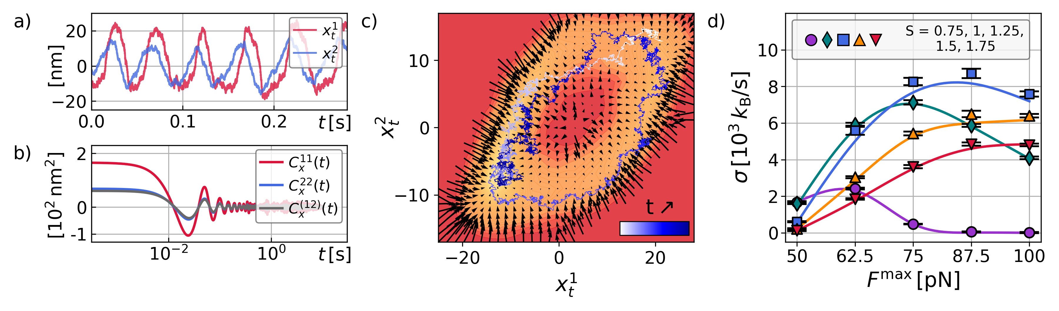
As shown in Fig. 2d, the predicted values (symbols) closely match the true values (solid lines). Since the system is nonlinear, the latter were numerically computed using Eq.(2). The accuracy of these estimates can be validated by the relative error, defined as . In all cases, the average error remains low at , except for instances where , where small denominators distort the error measure. The quality of these estimates is further supported by the accuracy metric , as detailed in Fig. S2a in [60]. On average, we find , with only three out of 25 cases where slightly exceeds 3. Crucially, the quality of our estimates remains unaffected by the average ion channel opening probability (Fig. S2b). In contrast, approaches based on trace irreversibility may encounter challenges when [48]. Another key observation is that, similar to the linear model, remains relatively constant ( to , see Fig. S2d in [60]) despite large variations in and , while spans orders of magnitude ( to ). This indicates that even in this highly nonlinear system, captures most of the information about the dissipative components of the dynamics.
Our method of estimating can be extended to the cases of partial observations when the diffusion matrix is diagonal. This is particularly important because, in most systems, only a subset of the dynamical degrees of freedom (DOFs) is observable. For example, in the hair-bundle model (12), it is very hard to directly observe the dynamics of molecular motors (that is, ). To address this issue, as detailed in Section S3 in [60], it is useful to decompose as
| (14) |
Each component is defined by , where denotes the -th coordinate of the mean local velocity (4), , and . From this, it follows
| (15) |
implying that any positive traffic component guarantees , indicating the system is out of equilibrium and providing a lower bound to the entropy production rate. This observation thus provides a practical method for detecting nonequilibrium and bounding potentially from a single stochastic trace. More in general, if only a subset of all DOFs is observable, one can select only positive traffic components and obtain a partial estimate of , namely
| (16) |
We note that estimating requires knowledge of the PDF of the entire system, making it impossible to derive from partial observations alone.
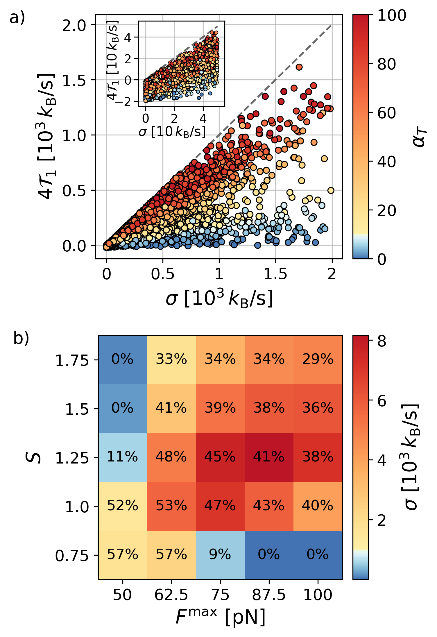
The Gaussian system (10), despite its simplicity, offers valuable insights when applying Eq. (15). Gaussian systems often pose challenges in detecting nonequilibrium states from irreversibility measurements [78, 79] or partial observations [80], especially without specific assumptions about the underlying model. In this context, our bound enables nonequilibrium detection from single traces under the minimal assumption of a diagonal diffusion matrix. Fig. 3a illustrates the relation between and for various parameters in (10), demonstrating that a higher ratio between the temperatures of the two thermal baths () tightens the bound, allowing for more precise nonequilibrium detection. Additionally, the condition corresponds to the absence of an equilibrium solution for (10) leading to the correlation function (see Section S7 in [60] for details). As a final remark, in our previous work [50], the red blood cell flickering traces we analyzed exhibited Gaussian statistics and a negative traffic component for the observed degree of freedom, which made it necessary to use a specific model for proper thermodynamic characterization of the system.
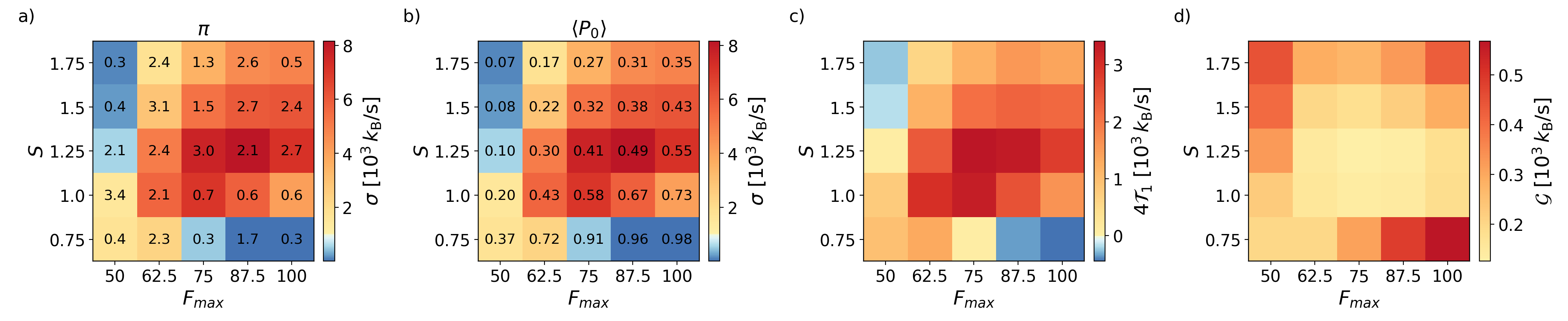
For the model (12), our bound yields the results shown in Fig. 3b. The colors of the heat map represent , while the numbers indicate the fraction of estimated using our method, specifically . In the more active regions of the parameter space, the inference procedure estimates roughly half of , demonstrating the method’s ability to capture a substantial portion of the system’s entropy production and emphasizing its potential for studying biological systems where complete data may be inaccessible.
To conclude, this Letter introduces the equation (5) to estimate from stochastic traces without needing the knowledge of forces. Implementing this technique in two different models, we demonstrate its accuracy and reliability in various scenarios (see Fig. 1d and Fig. 2d). When observations are partial, the lower bound (15), derived from our formula, aids in partially inferring dissipation, which is useful for examining nonequilibrium dynamics in biological systems such as hair cells (see Fig. 3b). For Gaussian systems with a diagonal diffusion constant, this criterion can detect nonequilibrium conditions even from stochastic data for a single degree of freedom. Overall, our approach offers a powerful and versatile framework for analyzing dissipation in nonequilibrium systems.
Acknowledgements.
ACKNOWLEDGMENTS The author thanks Marco Baiesi, Felix Ritort, Vincenzo Maria Schimmenti, Matteo Ciarchi, Daniel Maria Busiello and Edgar Roldan for useful discussions and feedback on the paper.References
- Maes [2003] C. Maes, On the origin and the use of fluctuation relations for the entropy, Séminaire Poincaré 2, 29 (2003).
- Seifert [2012] U. Seifert, Stochastic thermodynamics, fluctuation theorems and molecular machines, Reports on Progress in Physics 75, 126001 (2012).
- Peliti and Pigolotti [2021] L. Peliti and S. Pigolotti, Stochastic Thermodynamics: An Introduction (Princeton University Press, 2021).
- Gallavotti and Cohen [1995] G. Gallavotti and E. G. D. Cohen, Dynamical ensembles in nonequilibrium statistical mechanics, Phys. Rev. Lett. 74, 2694 (1995).
- Crooks [1999] G. E. Crooks, Entropy production fluctuation theorem and the nonequilibrium work relation for free energy differences, Phys. Rev. E 60, 2721 (1999).
- Kurchan [1998] J. Kurchan, Fluctuation theorem for stochastic dynamics, Journal of Physics A: Mathematical and General 31, 3719 (1998).
- Andrieux et al. [2007] D. Andrieux, P. Gaspard, S. Ciliberto, N. Garnier, S. Joubaud, and A. Petrosyan, Entropy production and time asymmetry in nonequilibrium fluctuations, Physical Review Letters 98, 150601 (2007).
- Li et al. [2019] J. Li, J. M. Horowitz, T. R. Gingrich, and N. Fakhri, Quantifying dissipation using fluctuating currents, Nature Communications 10, 1 (2019).
- Martínez et al. [2019] I. A. Martínez, G. Bisker, J. M. Horowitz, and J. M. Parrondo, Inferring broken detailed balance in the absence of observable currents, Nature Communications 10, 1 (2019).
- Ro et al. [2022] S. Ro, B. Guo, A. Shih, T. V. Phan, R. H. Austin, D. Levine, P. M. Chaikin, and S. Martiniani, Model-free measurement of local entropy production and extractable work in active matter, Physical Review Letters 129, 220601 (2022).
- Barato and Seifert [2015] A. C. Barato and U. Seifert, Thermodynamic Uncertainty Relation for Biomolecular Processes, Phys. Rev. Lett. 114, 158101 (2015).
- Pietzonka et al. [2017] P. Pietzonka, F. Ritort, and U. Seifert, Finite-time generalization of the thermodynamic uncertainty relation, Physical Review E 96, 012101 (2017).
- Macieszczak et al. [2018] K. Macieszczak, K. Brandner, and J. P. Garrahan, Unified thermodynamic uncertainty relations in linear response, Physical Review Letters 121, 130601 (2018).
- Busiello and Pigolotti [2019] D. M. Busiello and S. Pigolotti, Hyperaccurate currents in stochastic thermodynamics, Physical Review E 100, 060102 (2019).
- Hasegawa and Van Vu [2019a] Y. Hasegawa and T. Van Vu, Fluctuation theorem uncertainty relation, Physical review letters 123, 110602 (2019a).
- Hasegawa and Van Vu [2019b] Y. Hasegawa and T. Van Vu, Uncertainty relations in stochastic processes: An information inequality approach, Physical Review E 99, 062126 (2019b).
- Horowitz and Gingrich [2020] J. M. Horowitz and T. R. Gingrich, Thermodynamic uncertainty relations constrain non-equilibrium fluctuations, Nature Physics 16, 15 (2020).
- Otsubo et al. [2020] S. Otsubo, S. Ito, A. Dechant, and T. Sagawa, Estimating entropy production by machine learning of short-time fluctuating currents, Physical Review E 101, 062106 (2020).
- Falasco et al. [2020] G. Falasco, M. Esposito, and J.-C. Delvenne, Unifying thermodynamic uncertainty relations, New Journal of Physics 22, 053046 (2020).
- Terlizzi and Baiesi [2020] I. D. Terlizzi and M. Baiesi, A thermodynamic uncertainty relation for a system with memory, Journal of Physics A: Mathematical and Theoretical 53, 474002 (2020).
- Van Vu et al. [2020] T. Van Vu, Y. Hasegawa, et al., Entropy production estimation with optimal current, Physical Review E 101, 042138 (2020).
- Shiraishi [2021] N. Shiraishi, Optimal thermodynamic uncertainty relation in markov jump processes, Journal of Statistical Physics 185, 19 (2021).
- Van Vu et al. [2022] T. Van Vu, Y. Hasegawa, et al., Unified thermodynamic–kinetic uncertainty relation, Journal of Physics A: Mathematical and Theoretical 55, 405004 (2022).
- Dieball and Godec [2023] C. Dieball and A. Godec, Direct route to thermodynamic uncertainty relations and their saturation, Physical Review Letters 130, 087101 (2023).
- Pietzonka and Coghi [2024] P. Pietzonka and F. Coghi, Thermodynamic cost for precision of general counting observables, Physical Review E 109, 064128 (2024).
- Turlier et al. [2016] H. Turlier, D. A. Fedosov, B. Audoly, T. Auth, N. S. Gov, C. Sykes, J.-F. Joanny, G. Gompper, and T. Betz, Equilibrium physics breakdown reveals the active nature of red blood cell flickering, Nature Physics 12, 513 (2016).
- Wang [2018] S.-W. Wang, Inferring energy dissipation from violation of the fluctuation-dissipation theorem, Physical Review E 97, 052125 (2018).
- Harada and Sasa [2005] T. Harada and S. Sasa, Equality connecting energy dissipation with violation of fluctuation-response relation, Phys. Rev. Lett. 95, 130602 (2005).
- Sekimoto [1998] K. Sekimoto, Langevin equation and thermodynamics, Progress of Theoretical Physics Supplement 130, 17 (1998).
- Gnesotto et al. [2018] F. S. Gnesotto, F. Mura, J. Gladrow, and C. P. Broedersz, Broken detailed balance and non-equilibrium dynamics in living systems: a review, Reports on Progress in Physics 81, 066601 (2018).
- Roldán and Parrondo [2012] É. Roldán and J. M. Parrondo, Entropy production and Kullback-Leibler divergence between stationary trajectories of discrete systems, Physical Review E 85, 031129 (2012).
- Bisker et al. [2017] G. Bisker, M. Polettini, T. R. Gingrich, and J. M. Horowitz, Hierarchical bounds on entropy production inferred from partial information, Journal of Statistical Mechanics: Theory and Experiment 2017, 093210 (2017).
- Busiello et al. [2019] D. M. Busiello, J. Hidalgo, and A. Maritan, Entropy production for coarse-grained dynamics, New Journal of Physics 21, 073004 (2019).
- Skinner and Dunkel [2021a] D. J. Skinner and J. Dunkel, Estimating entropy production from waiting time distributions, Physical Review Letters 127, 198101 (2021a).
- Skinner and Dunkel [2021b] D. J. Skinner and J. Dunkel, Improved bounds on entropy production in living systems, Proceedings of the National Academy of Sciences 118, e2024300118 (2021b).
- Teza and Stella [2020] G. Teza and A. L. Stella, Exact coarse graining preserves entropy production out of equilibrium, Physical Review Letters 125, 110601 (2020).
- Ghosal and Bisker [2023] A. Ghosal and G. Bisker, Entropy production rates for different notions of partial information, Journal of Physics D: Applied Physics 56, 254001 (2023).
- Harunari et al. [2022] P. E. Harunari, A. Dutta, M. Polettini, and É. Roldán, What to learn from a few visible transitions’ statistics?, Physical Review X 12, 041026 (2022).
- Van der Meer et al. [2022] J. Van der Meer, B. Ertel, and U. Seifert, Thermodynamic inference in partially accessible markov networks: a unifying perspective from transition-based waiting time distributions, Physical Review X 12, 031025 (2022).
- Blom et al. [2024] K. Blom, K. Song, E. Vouga, A. Godec, and D. E. Makarov, Milestoning estimators of dissipation in systems observed at a coarse resolution, Proceedings of the National Academy of Sciences 121, e2318333121 (2024).
- Baiesi et al. [2024] M. Baiesi, T. Nishiyama, and G. Falasco, Effective estimation of entropy production with lacking data, Communications Physics 7, 264 (2024).
- Gingrich et al. [2017] T. R. Gingrich, G. M. Rotskoff, and J. M. Horowitz, Inferring dissipation from current fluctuations, Journal of Physics A: Mathematical and Theoretical 50, 184004 (2017).
- Dieball and Godec [2022a] C. Dieball and A. Godec, Mathematical, thermodynamical, and experimental necessity for coarse graining empirical densities and currents in continuous space, Physical Review Letters 129, 140601 (2022a).
- Dieball and Godec [2022b] C. Dieball and A. Godec, Coarse graining empirical densities and currents in continuous-space steady states, Physical Review Research 4, 033243 (2022b).
- Ghosal and Bisker [2022] A. Ghosal and G. Bisker, Inferring entropy production rate from partially observed langevin dynamics under coarse-graining, Physical Chemistry Chemical Physics 24, 24021 (2022).
- Roldán and Parrondo [2010] É. Roldán and J. M. Parrondo, Estimating dissipation from single stationary trajectories, Physical review letters 105, 150607 (2010).
- Gnesotto et al. [2020] F. S. Gnesotto, G. Gradziuk, P. Ronceray, and C. P. Broedersz, Learning the non-equilibrium dynamics of brownian movies, Nature communications 11, 5378 (2020).
- Roldán et al. [2021] É. Roldán, J. Barral, P. Martin, J. M. Parrondo, and F. Jülicher, Quantifying entropy production in active fluctuations of the hair-cell bundle from time irreversibility and uncertainty relations, New Journal of Physics 23, 083013 (2021).
- Busiello et al. [2024a] D. M. Busiello, M. Ciarchi, and I. Di Terlizzi, Unraveling active baths through their hidden degrees of freedom, Physical Review Research 6, 013190 (2024a).
- Terlizzi et al. [2024] I. D. Terlizzi, M. Gironella, D. Herraez-Aguilar, T. Betz, F. Monroy, M. Baiesi, and F. Ritort, Variance sum rule for entropy production, Science 383, 971 (2024).
- Di Terlizzi et al. [2024] I. Di Terlizzi, M. Baiesi, and F. Ritort, Variance sum rule: proofs and solvable models, New Journal of Physics (2024).
- Tucci et al. [2022] G. Tucci, E. Roldán, A. Gambassi, R. Belousov, F. Berger, R. G. Alonso, and A. J. Hudspeth, Modeling active non-markovian oscillations, Phys. Rev. Lett. 129, 030603 (2022).
- Hyvärinen and Dayan [2005] A. Hyvärinen and P. Dayan, Estimation of non-normalized statistical models by score matching., Journal of Machine Learning Research 6 (2005).
- Song et al. [2020] Y. Song, S. Garg, J. Shi, and S. Ermon, Sliced score matching: A scalable approach to density and score estimation, in Uncertainty in Artificial Intelligence (PMLR, 2020) pp. 574–584.
- Song et al. [2021] Y. Song, C. Durkan, I. Murray, and S. Ermon, Maximum likelihood training of score-based diffusion models, Advances in neural information processing systems 34, 1415 (2021).
- Kim et al. [2022] D. Kim, S. Shin, K. Song, W. Kang, and I.-C. Moon, Soft truncation: A universal training technique of score-based diffusion model for high precision score estimation, in Proceedings of the 39th International Conference on Machine Learning (ICML), Proceedings of Machine Learning Research, Vol. 162 (PMLR, 2022) pp. 11388–11403.
- Biroli and Mézard [2023] G. Biroli and M. Mézard, Generative diffusion in very large dimensions, Journal of Statistical Mechanics: Theory and Experiment 2023, 093402 (2023).
- Biroli et al. [2024] G. Biroli, T. Bonnaire, V. De Bortoli, and M. Mézard, Dynamical regimes of diffusion models, Nature Communications 15, 9957 (2024).
- Boffi and Vanden-Eijnden [2024] N. M. Boffi and E. Vanden-Eijnden, Deep learning probability flows and entropy production rates in active matter, Proceedings of the National Academy of Sciences 121, e2318106121 (2024).
- Di Terlizzi [2025] I. Di Terlizzi, Supplemental material for "Force-free entropy production estimation from stochastic traces" (2025).
- Baiesi and Falasco [2015] M. Baiesi and G. Falasco, Inflow rate, a time-symmetric observable obeying fluctuation relations, Phys. Rev. E 92, 042162 (2015).
- Frishman and Ronceray [2020] A. Frishman and P. Ronceray, Learning force fields from stochastic trajectories, Physical Review X 10, 021009 (2020).
- Maes et al. [2008] C. Maes, K. Netočnỳ, and B. Wynants, Steady state statistics of driven diffusions, Physica A: Statistical Mechanics and its Applications 387, 2675 (2008).
- Baiesi and Maes [2018] M. Baiesi and C. Maes, Life efficiency does not always increase with the dissipation rate, Journal of Physics Communications 2, 045017 (2018).
- Di Terlizzi and Baiesi [2019] I. Di Terlizzi and M. Baiesi, Kinetic uncertainty relation, J. Phys. A: Math. Theor. 52, 02LT03 (2019).
- Maes [2020] C. Maes, Frenesy: Time-symmetric dynamical activity in nonequilibria, Physics Reports 850, 1 (2020).
- Martin et al. [2003] P. Martin, D. Bozovic, Y. Choe, and A. J. Hudspeth, Spontaneous oscillation by hair bundles of the bullfrog’s sacculus, Journal of Neuroscience 23, 4533 (2003).
- Crisanti et al. [2012] A. Crisanti, A. Puglisi, and D. Villamaina, Nonequilibrium and information: The role of cross correlations, Phys. Rev. E 85, 061127 (2012).
- Dotsenko et al. [2013] V. Dotsenko, A. Maciołek, O. Vasilyev, and G. Oshanin, Two-temperature langevin dynamics in a parabolic potential, Phys. Rev. E 87, 062130 (2013).
- Mancois et al. [2018] V. Mancois, B. Marcos, P. Viot, and D. Wilkowski, Two-temperature Brownian dynamics of a particle in a confining potential, Phys. Rev. E 97, 052121 (2018).
- Cerasoli et al. [2018] S. Cerasoli, V. Dotsenko, G. Oshanin, and L. Rondoni, Asymmetry relations and effective temperatures for biased Brownian gyrators, Phys. Rev. E 98, 042149 (2018).
- Loos and Klapp [2020] S. A. M. Loos and S. H. Klapp, Irreversibility, heat and information flows induced by non-reciprocal interactions, New Journal of Physics 22, 123051 (2020).
- Busiello et al. [2024b] D. M. Busiello, M. Ciarchi, and I. Di Terlizzi, Unraveling active baths through their hidden degrees of freedom, Phys. Rev. Res. 6, 013190 (2024b).
- Tinevez et al. [2007] J.-Y. Tinevez, F. Jülicher, and P. Martin, Unifying the various incarnations of active hair-bundle motility by the vertebrate hair cell, Biophysical Journal 93, 4053 (2007).
- Barral et al. [2018] J. Barral, F. Jülicher, and P. Martin, Friction from transduction channels’ gating affects spontaneous hair-bundle oscillations, Biophysical Journal 114, 425 (2018).
- Bormuth et al. [2014] V. Bormuth, J. Barral, J.-F. Joanny, F. Jülicher, and P. Martin, Transduction channels’ gating can control friction on vibrating hair-cell bundles in the ear, Proceedings of the National Academy of Sciences 111, 7185 (2014).
- Nadrowski et al. [2004] B. Nadrowski, P. Martin, and F. Jülicher, Active hair-bundle motility harnesses noise to operate near an optimum of mechanosensitivity, Proceedings of the National Academy of Sciences 101, 12195 (2004).
- Zamponi et al. [2005] F. Zamponi, F. Bonetto, L. F. Cugliandolo, and J. Kurchan, A fluctuation theorem for non-equilibrium relaxational systems driven by external forces, Journal of Statistical Mechanics: Theory and Experiment 2005, P09013 (2005).
- Caprini et al. [2019] L. Caprini, U. M. B. Marconi, A. Puglisi, and A. Vulpiani, The entropy production of ornstein–uhlenbeck active particles: a path integral method for correlations, Journal of Statistical Mechanics: Theory and Experiment 2019, 053203 (2019).
- Lucente et al. [2022] D. Lucente, A. Baldassarri, A. Puglisi, A. Vulpiani, and M. Viale, Inference of time irreversibility from incomplete information: Linear systems and its pitfalls, Physical Review Research 4, 043103 (2022).
Supplemental Material for
Force-free entropy production estimation from stochastic traces
I. Di Terlizzi
Max Planck Institute for the Physics of Complex Systems, Nöthnitzer Straße 38, 01187, Dresden, Germany
S1 Main result derivation
This section is devoted to the derivation of the main result (5). As a starting point, we consider the Langevin equations
| (S1) |
where, using Einstein’s summation convention, we define the drift for simplicity and the Gaussian noise has first and second moments given by and . The associated Fokker-Planck equation is given by
| (S2) |
where represents the probability current, and is the mean local velocity. At equilibrium, the probability current vanishes, , leading to a stationary probability density function (PDF) where . In contrast, a nonequilibrium steady state (NESS) is characterized by non-zero, irrotational probability currents satisfying , which also results in a time-independent PDF.
The variance sum rule [50, 51] for the displacement and the drift is
| (S3) |
where denotes the symmetrisation of indexes and . As shown in [51], this formula holds for a diffusion matrix that can be expressed in either of the following forms: , where is the temperature and is an arbitrary positive-definite symmetric mobility matrix, or , where is a diagonal matrix of temperatures and is a diagonal mobility matrix. From a practical point of view, the drifts are usually be difficult to measure in experiments. Hence, we aim to replace them with functions of the effective potential
| (S4) |
which, we assume, can be estimated from recorded trajectories. In particular, we consider the effective forces introduced above as the gradient of ,
| (S5) |
and the related "Fick" velocities
| (S6) |
In this way, the drift
| (S7) |
is interpreted as a sum of the local mean velocity and the Fick velocity . The VSR is rewritten as
| (S8) |
and then use (S1) to replace and then (S7) to replace the drift . Thus, the term in the integral becomes
| (S9) |
and we may rewrite the VSR as
| (S10) |
The second time derivative of (S1), evaluated at time ,
| (S11) |
contains a term that we may re-cast as because in a NESS. Introducing is convenient because the entropy production rate is the weighted sum of such terms,
| (S12) |
Hence, using (S11), we rewrite (S12) as
| (S13) |
By using that, in a NESS,
| (S14) |
where denotes symmetrised indexes, along with (S6), we may also rewrite (S13) as
| (S15) |
to highlight the presence of the traffic and inflow rate in the formula. Note that is the trace operator, denotes the symmetrized matrix, and that, since is symmetric, it follows that , as the contraction of the antisymmetric part of a tensor with a symmetric tensor is zero.
S2 Proof that
We start from the definition of traffic presented in [63]:
| (S16) |
By plugging (Eq. (S7)) in the first term on the right hand side, and by using the definition of in (S12), one gets
| (S17) |
For the second term on the right-hand side, it follows directly that
| (S18) |
where we have used the fact that decays sufficiently rapidly at infinity and that in a NESS, as discussed after Eq. (S2). Moreover, by using the definition of
| (S19) |
where again we leveraged the rapid decay of at infinity and the propriety that in a NESS. By finally combining (S17) and (S19) we get
| (S20) |
which compared to Eq. (S15) concludes the proof.
S3 Partial observations and bounds for diagonal
We start from our main result (5) for the particular case of a diagonal diffusion matrix . In this case, following the derivation in Section S1, one can write as
| (S21) |
where the equality holds component-wise with terms given by
| (S22) |
As a first consequence of this component-wise relationship is that
| (S23) |
implying that, whenever a traffic component is bigger that zero, it also means that is non-zero and the system is out of equilibrium. This is a very important feature of (S21) as it enables the detection of non-equilibrium even from a single stochastic trace and provides a practical way to lower bound the entropy production rate. This result generalises the criterion presented in [51] for which, if is positive, then is large and the system is strongly out of equilibrium. Indeed, the latter argument, could only be applied if all degrees of freedom can be observed. Here instead, one can rely on limited observations of a subset of all DOFs, select only positive traffic components and get a partial estimate of , namely
| (S24) |
We stress that, in order to estimate one needs the complete PDF of the whole system and hence, it can not be estimated from partial observations.
To conclude this section, we compare Eq. (S21) with the expression for derived in [50, 51], which is given by
| (S25) |
where, as before, the equality holds component-wise. Here, , , and denote the force, mobility, and temperature associated with the degree of freedom (DOF), respectively. In this case, the term represents the heat flux transferred to the environment by the DOF. Notably, this component can be either positive or negative depending on the direction of the flow. This implies that measuring microscopic forces allows the determination of DOF-specific heat fluxes, which cannot be achieved by relying solely on traffic and effective forces. However, while Eq. (S25) provides insights into these specific fluxes, it does not allow the derivation of thermodynamic bounds, such as those established in Eq. (S24).
S4 Proof that
The prove that , we start by considering the discretised form of the Langevin equations (S1)
| (S26) |
where is a Wiener process with average and variance given by and . By taking the averaged cross product of and components of (S26) one gets
| (S27) |
where, again, denotes symmetrised indexes and is the symmetrised correlation matrix for the observable . Note that correlation functions are homogeneous in time due to the steady-state dynamics of the system. Using further the symmetry of the diffusion matrix and performing a Taylor expansion of for small and keeping only terms of order , it immediately follows that .
S5 2D linear model
In this section we analytically solve the linear 2D system presented in the main text with dynamical equations given by
| (S28) |
S5.1 Equal time correlation matrix
The first step consists in calculating the components of the the equal time correlation matrix which can be done by considering the discretised form of Eq. (S28) whic reads
| (S29) |
where represents a Wiener process characterized by a mean of and a variance of . By squaring and taking the cross product of the equations in (S29), followed by averaging and retaining only terms of order , we obtain:
| (S30) |
where we used that , . Note these three equations univocally determine the components of which is symmetric in a NESS. In particular,
| (S31) |
whose solution is:
| (S32) |
namely the components of the equal time correlation matrix .
S5.2 Time dependent correlation matrix
To compute the time-dependent correlation matrix , we multiply each equation in (S28), evaluated at a time , by and evaluated at , and then take the ensemble average, resulting in:
| (S33) |
where we used that for . To solve this linear system of differential equations, we resort to standard procedure based on Laplace transform, which leads to
| (S34) |
where is the Laplace transform of . In the time domain, the corresponding expressions are:
| (S35) | |||||
where . By combining (S32) with (S5.2), one can readily evaluate first and second time derivative of the correlation matrix at time . In particular, for first derivatives one gets
| (S36) |
for which it holds that , as expected. Finally, for second derivatives, one gets:
| (S37) |
S5.3 Effective forces and inflow rate
Effective forces in a NESS can be easily estimated for this linear system as the probability distribution is Gaussian,
| (S38) |
where stands for the determinant. Hence, the effective forces become
| (S39) |
With some algebraic manipulation, this enables the calculation of the correlation matrix for the effective forces, , which is essential for determining the inflow rate, . The components of the symmetric matrix are given by:
| (S40) |
Because the diffusion matrix is diagonal, with and , the inflow rate reduces to:
| (S41) |
as anticipated in the main text.
S5.4 Entropy production
The entropy production rate associated to the system can be calculated using the standard formula in Eq. (2) presented in the main text. By identifying the forces acting on the the degrees of freedom
| (S42) |
Eq. (2) can be readily be evaluated as
| (S43) |
because in a NESS. By further plugging in the dynamical equations form (S28) into (S43) one finally gets gets
| (S44) |
where we used the results in (S32) and that only has diagonal terms, as shown in Section S6.
S6 Proof that
In this section, we aim to compute the correlation , where the symbol denotes the Stratonovich product, for a system of Langevin equations as in Eq. (S1):
| (S45) |
with and . In the Stratonovich interpretation, the stochastic integral evaluates at the midpoint of the integration interval, introducing a correlation between the variable and the noise . To compute , we use the formal solution of the Langevin equation:
| (S46) |
At short times, the dominant contribution to arises from the noise term as , while the deterministic term contributes only to longer timescales. Thus, for small , the dynamics of can be approximated as:
| (S47) |
Using this approximate form of , and by multiplying both sides by , one gets:
| (S48) |
where we used . Within the Stratonovich convention, integrating the Dirac delta function centered at one of the integration limits gives
| (S49) |
which finally implies that (S48) becomes
| (S50) |
S7 Non existence of equilibrium solutions for 2D linear model
The problem of detecting the nonequilibrium nature of a one-dimensional Gaussian stochastic process can be effectively addressed within the framework of the 2D linear model (10) discussed in this paper. Following the approach in [80], we consider the scenario where only one of the two degrees of freedom (DOFs) in (10) is observed, for example . This implies that only the autocorrelation function can be inferred from the data. Since the system is Gaussian, the propagator of the associated Fokker-Planck equation is also Gaussian, meaning that the system is fully characterized by the two-point correlation function. Assuming is computed and the data is modeled by (10), one could attempt to fit the model parameters and infer directly, hence determining whether or not the process is irreversible or not. However, even if the system is out of equilibrium, there exist certain parameter regimes where inferring nonequilibrium behavior becomes impossible. Specifically, we will show that in regimes where the correlation function exhibits positive concavity (i.e., ), there always exists a set of parameters for which the system appears to be in equilibrium, reproducing the exact measured correlation function. This degeneracy renders the inference of nonequilibrium behavior ambiguous. We further demonstrate that when , in agreement with our result (16), detection of the nonequilibrium nature of a 1D Gaussian stochastic process becomes feasible. This arises because in such cases, no parameter set exists that generates a system at equilibrium while remaining compatible with the observed correlation function. To establish this, we express in Fourier space, leveraging the relation between Laplace and Fourier transforms:
| (S51) |
where we utilize Eq. (LABEL:eq:asym_2D_corr_laplace_sol). The coefficients, which can be experimentally estimated from the data, are given by:
| (S52) | ||||
with , and to ensure the existence of a nonequilibrium steady state (NESS). This implies that any combination of , , , , , and producing the observed values in (S52) is a potential candidate for the true set of system parameters. We now investigate the conditions under which a parameter set yielding an equilibrium system can solve the equations in (S52). Assuming the two DOFs in (10) are coupled (i.e., ), the system can be at equilibrium if and only if , as must be positive. Under this condition, (S52) simplifies to:
| (S53) | ||||
Through algebraic manipulation, we find that this leads to the following condition for :
| (S54) |
which must satisfy to guarantee the stability of the equilibrium solution. Indeed, if , then must be negative to ensure . But this would mean that , as , ruling out a stable equilibrium. As a consequence, if for example the measured satisfies:
| (S55) |
which could occur with a sufficiently large (as it does not affect , , or ), this would result in . This disrupts the existence of a stationary equilibrium, meaning that imposing equilibrium conditions on the system in (S53) leads to a contradiction and therefore the observed correlation function is incompatible with equilibrium dynamics. More generally, this incompatibility arises whenever the right-hand side of (S54) is positive, which corresponds to:
| (S56) |
as can be shown using the expressions for the first and second derivatives of in (S36) and (LABEL:eq:lin_sec_der), along with the definition of traffic components, namely . In other words, because at equilibrium , a measured can still yield , thus keeping the system compatible with equilibrium. Conversely, if , the condition cannot be satisfied, indicating that the system must be out of equilibrium.
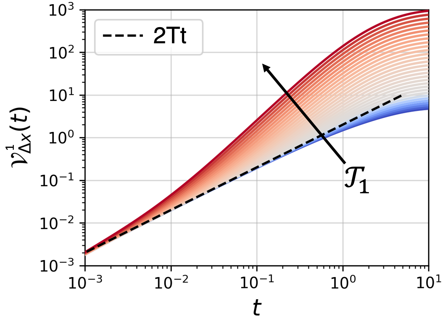
To conclude this section, we visually illustrate in Fig. S1 how the behavior of the displacement variance, , evolves as increases. This term corresponds to the first component on the right-hand side of the VSR (S3). As increases, we observe an enhanced diffusion compared to the baseline provided by normal diffusion (represented by the solid black line).
S8 Hair-cell model
The spontaneous oscillations of hair bundles in the auditory organs of bullfrogs are driven by the interplay of mechanosensitive ion channels, molecular motor activity, and calcium feedback mechanisms. These dynamics, derived and discussed in [67, 74, 75, 76, 48], are effectively captured by a model with two degrees of freedom: the bundle position and the center of mass of the molecular motors . Following [48], in this section, we provide a brief overview of the key equations governing the system’s evolution. We outline the roles of potential , active force , and effective temperature , highlighting their contributions to the nonequilibrium nature of the system.
The system’s equations are:
| (S57) |
where the potential accounts for elastic forces and mechanosensitive ion channels. The explicit form of is given by:
| (S58) |
where and are mobility coefficients, and are stiffness coefficients, is the gating swing of a transduction channel, and
| (S59) |
Here, represents the energy difference between the open and closed states of the channels, and is the number of transduction elements. The nonequilibrium behavior is driven by molecular motor activity, which is encoded in the effective temperature and the non-conservative force:
| (S60) |
The parameter quantifies calcium-mediated feedback on the motor force, and the open probability of the transduction channels is given by:
| (S61) |
This expression for represents the open probability of a two-state equilibrium model of a channel, where the difference in free energy between the open and closed states depends linearly on the distance .
In the main text we discussed the application of our method to simulated traces with fixed parameters. These are set to are set to: , , , , , and . Furthermore, in Fig.S2, we present additional results that illustrate the behavior of the system as a function of and . Panel a) shows a heat map of , with accuracy displayed above each combination of parameters to quantify the reliability of our estimates. Panel b) presents the heatmap of , displaying a color pattern that closely resembles that of panel a). This similarity demonstrates how dissipation is effectively captured and encoded within the traffic components. Finally, panel c) illustrates the inflow rate , which exhibits markedly lower variability compared to and across all combinations of parameters. Furthermore, the values of are significantly lower than the maximum observed in panel a), reinforcing the conclusion that information about the dissipative processes is primarily encoded in the traffic , rather than in the inflow .
S9 Data analysis
The estimation process involves two essential steps to derive the entropy production rate from a single stochastic trace using Eq.(5). First, the short-time first and second derivatives of the correlation functions, and , are computed. As Appendix S4 outlines, the first derivative determines the diffusion matrix , which is needed to calculate both terms in the main equation (5). The second step calculates the inflow rate , which instead focuses on calculating the correlation matrix of the effective forces , .
S9.1 Estimation of derivatives
For the first task, each component of the position correlation matrix is fitted with a sum of an appropriate, system-dependent number of exponentials:
| (S62) |
where are the amplitudes and the system’s typical timescales. From this representation, the short-time derivatives can be derived analytically:
| (S63) |
In practice, it is sufficient to fit only the components of the symmetric correlation matrix, as these are the only terms required in the relevant formulas. This approach eliminates the need for numerical differentiation, which is particularly susceptible to noise in stochastic data. For clarity, the component indices will also be omitted from the formulas hereafter.
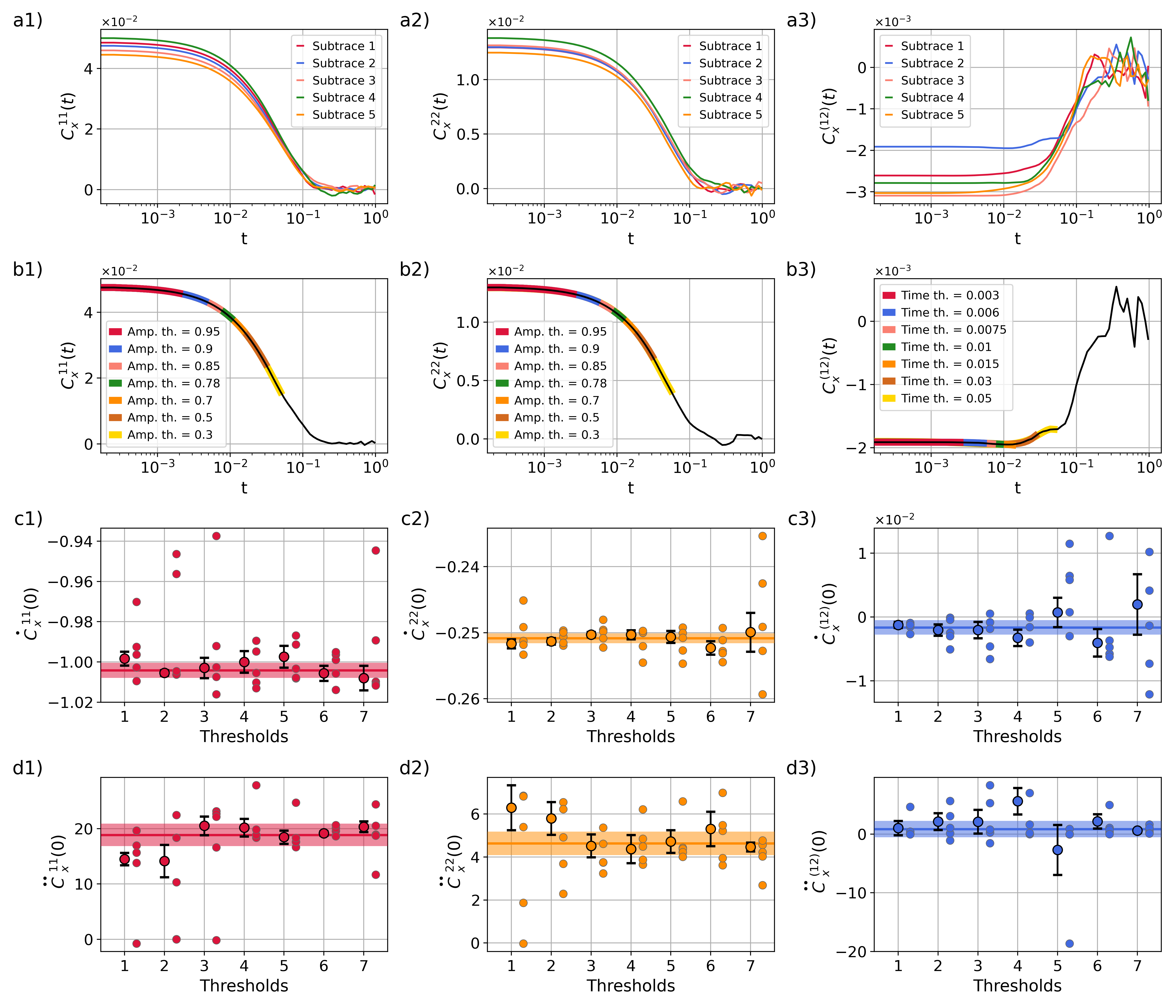
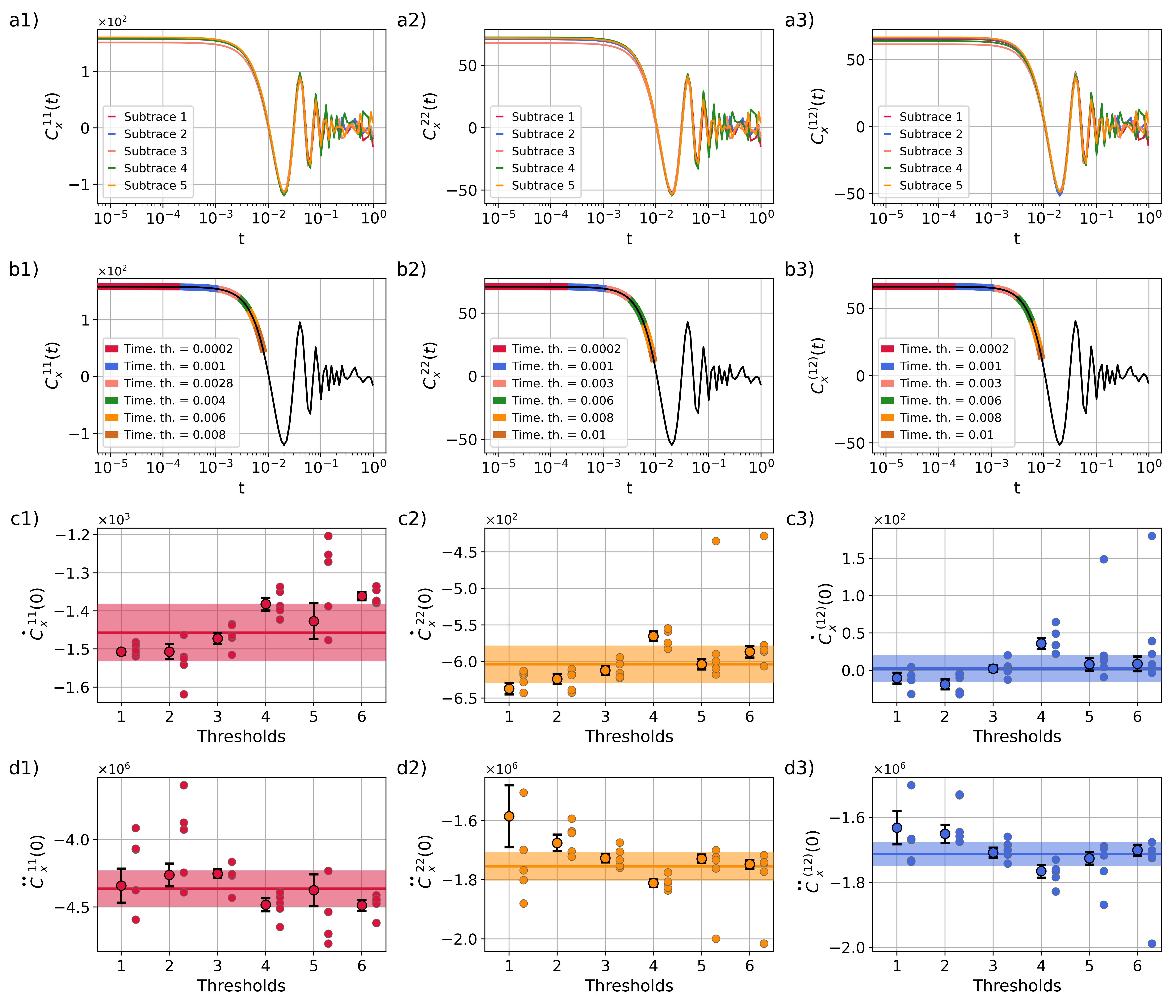
The stochastic trace is split into subtraces to ensure robustness, with each subtrace analyzed independently. For each subtrace, position correlation functions are numerically calculated over a predefined time window, see first row in Figures S3 and S4. A threshold-based approach is applied to select data points for fitting. These thresholds are defined as either a fraction of the initial amplitude of the correlation function or as a cut-off in time, depending on the shape of the correlation functions.
The fitting process determines the parameters and for each subtrace and threshold. The fit results are shown in the second row of Figures S3 and S4 for a selected subtrace and all chosen thresholds, where the correlation functions are plotted along with their exponential fits, illustrating the data and model agreement. The quality of the fits is then evaluated using a residual metric, denoted by , defined as:
| (S64) |
where is the number of data points in time, is the number of degrees of freedom, is the number of fitting parameters, is the observed correlation at time , and is the corresponding fitted value.
In many applications, residual metrics like are normalized by dividing the squared residuals by to weight the contribution of each point proportionally to its magnitude. However, this normalization is not used here because it leads to instability when approaches zero. By avoiding this normalization, the residual metric ensures a robust evaluation of fit quality without overweighting regions where correlation functions are close to zero. The inclusion of adjusts for the degrees of freedom in the fit but does not affect the computation of averages or variances in subsequent steps, as we take to be the same for all subtraces at a given threshold. The squared inverse of this metric, , is then used as the weight for each fit at a fixed threshold, ensuring that more reliable fits contribute more significantly to the initial estimates of and .
As a result, at each threshold, the derivative estimates across all subtraces are combined using a weighted averaging procedure. Specifically, the weighted mean for a derivative , estimated through Eq. (S63) with the fitted parameters, is calculated as:
| (S65) |
where is the estimate for a particular subtrace, and is the associated weight derived from the residual metric. The variance of the weighted mean is calculated as:
| (S66) |
We further combine these values to produce the final estimate of and . This is achieved using the same weighted averaging procedure, treating the threshold-specific means as individual estimates and their variances as the basis for weights. The final weighted mean is computed as:
| (S67) |
where is the weight derived from the threshold-specific variance. The variance of the weighted mean is calculated analogously:
| (S68) |
with the standard error given by , where is the number of chosen thresholds.
The results of this two-level averaging procedure are shown in the third and fourth row of Figures S3 and S4. The derivative estimates for all thresholds are also displayed, with weighted averages and their uncertainties highlighted to confirm the reliability and consistency of the approach.
By splitting stochastic traces into subtraces and aggregating results first across subtraces and then across thresholds, this two-level averaging procedure provides robust and reliable estimates of and . By finally using that , we can readily calculate the term in (5) with estimate errors calculated with the error propagation formula.
S9.2 Estimation of effective forces
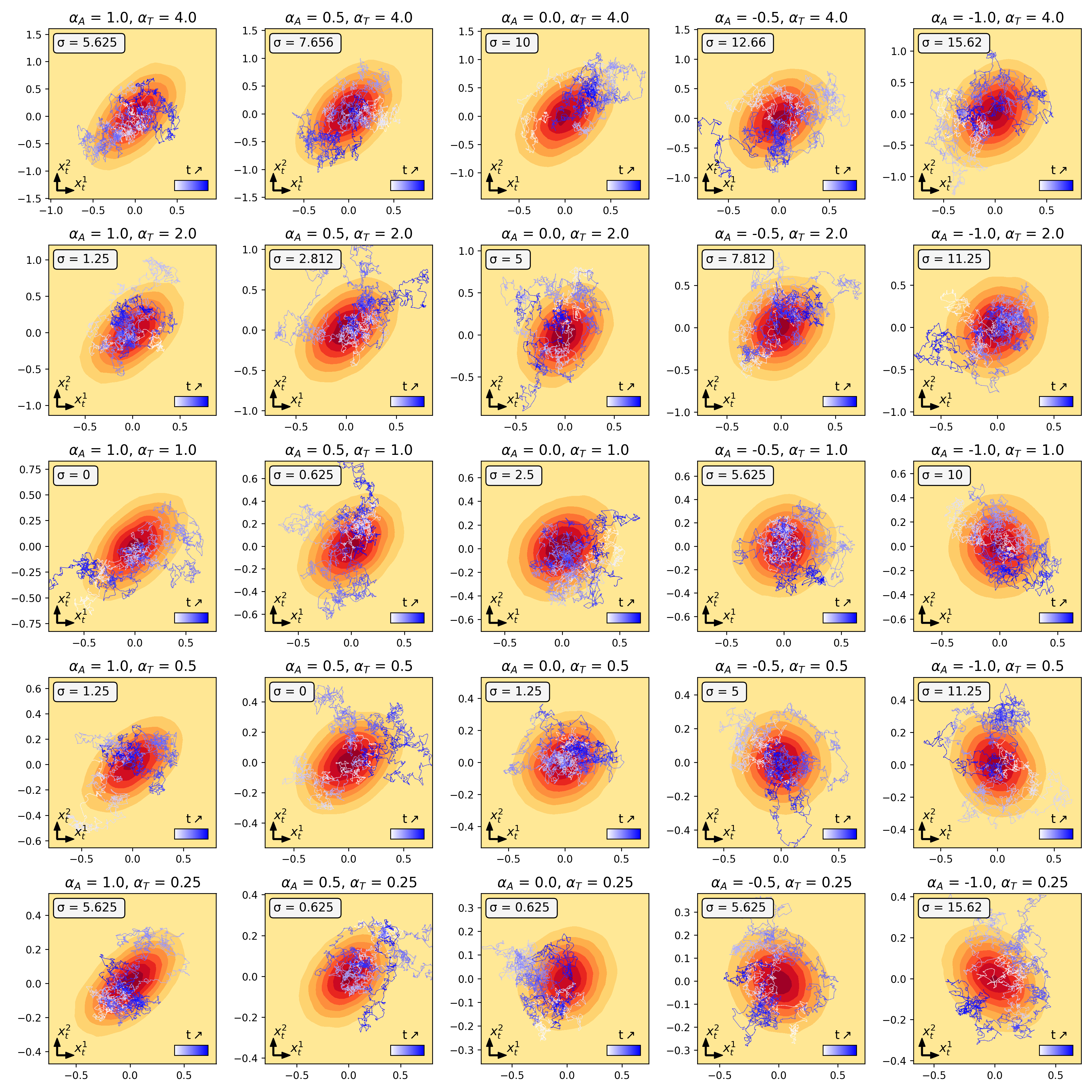
To calculate the inflow rate , we first estimate the covariance matrix of the effective forces associated with the system. This is done by estimating the joint probability distribution of the observed stochastic trace using non-parametric kernel density estimation. Figures S5 and S6 show the estimated probability density functions alongside a segment of the trajectories for all traces analyzed in the paper. Note that, especially for the bullfrog hair cell model, the traces exhibiting a higher degree of circulation correspond to those with a higher entropy production rate . To enhance robustness, the trajectory data is divided into smaller independent subtraces, which are processed individually. For each subtrace, the numerical gradient of the logarithm of the estimated is computed to derive the effective forces. The force covariance matrix is computed by averaging the estimated vector field, as shown, for example, in Figures 1c and 2c, weighted by the estimated probability density function . To enhance the accuracy of the final estimates, the results from all subtraces are averaged. The uncertainty in these estimates is quantified using the standard error.
The inflow rate is then calculated in a straightforward way, and its statistical error is determined using the error propagation formula. Finally, this result is combined with the outcomes of the previous analysis to compute and its associated statistical error, again using the error propagation formula.