Training Deep Learning Models with Norm-Constrained LMOs
Abstract
In this work, we study optimization methods that leverage the linear minimization oracle () over a norm-ball. We propose a new stochastic family of algorithms that uses the to adapt to the geometry of the problem and, perhaps surprisingly, show that they can be applied to unconstrained problems. The resulting update rule unifies several existing optimization methods under a single framework. Furthermore, we propose an explicit choice of norm for deep architectures, which, as a side benefit, leads to the transferability of hyperparameters across model sizes. Experimentally, we demonstrate significant speedups on nanoGPT training without any reliance on Adam. The proposed method is memory-efficient, requiring only one set of model weights and one set of gradients, which can be stored in half-precision.
.tocmtchapter \etocsettagdepthmtchaptersubsection \etocsettagdepthmtappendixnone
1 Introduction
| Method | Problem | constraint set | Reference | ||
| Normalized SGD | Unconstrained | Euclidean -ball | (Hazan et al., 2015) | ||
| Momentum Normalized SGD | Unconstrained | Euclidean -ball | (Cutkosky & Mehta, 2020) | ||
| SignSGD | Unconstrained | Max-norm -ball | (Bernstein et al., 2018, Thm. 1)2 | ||
| Signum | Unconstrained | Max-norm -ball | (Bernstein et al., 2018, Thm. 3)2 | ||
| Muon1 | Unconstrained | Spectral -ball | (Jordan et al., 2024b) |
1 With non-Nesterov based momentum.
2 The theoretical guarantee relies on increasing batch size.
Deep learning has greatly benefited from adaptive optimization methods such as RMSProp (Hinton et al., 2012), AdaGrad (Duchi et al., 2011; McMahan & Streeter, 2010), and Adam (Kingma, 2014), which dynamically change the geometry of the problem based on gradients encountered on-the-fly during training. While these methods have demonstrated remarkable success, they fundamentally treat neural networks (NNs) as optimization problems where we lack any prior knowledge about their particular setting.
However, NNs are far from being black boxes—their structure is not only known but they are deliberately designed. This simple observation raises directly the question:
Is it more beneficial to adapt the optimizer a priori, instead of exploring their respective geometries on-the-fly?
Adaptation on-the-fly has been the defacto standard in this setting, with adaptive algorithms, such as Adam (Kingma, 2014), dominating the deep learning model training.
One possible way for adaptation a priori, which we focus on in this work, is to modify the underlying norm used to measure distances in the parameter space. There is precedence to our proposal, as the early work by Carlson et al. (2015a, b, c) introduced the stochastic spectral descent method (SSD), which performs steepest descent in the spectral norm, and demonstrated that the method can substantially accelerate deep learning training.
The significance of the SSD approach has been very recently brought back to attention by Bernstein & Newhouse (2024b), who showed that the Shampoo optimizer (Gupta et al., 2017)—winner of the external tuning track at the 2024 AlgoPerf: Training Algorithms competition (Dahl et al., 2023)—can be viewed as SSD when a certain accumulation is disabled. Moreover, Bernstein & Newhouse (2024b) introduced an efficient Newton-Schultz iteration to replace the approximate SVD calculations previously required. Jordan et al. (2024b) incorporated the Newton-Schultz iteration with additional momentum into SSD under the name Muon to achieve impressive results on the nanoGPT architecture by applying it to the hidden layers.
Contributions
This work focuses on developing an algorithmic framework that can exploit an appropriate choice of norm for the entire neural network with particular emphasis on hyperparameter transfer across model sizes (Yang & Hu, 2021), convergence and practical performance.
To adapt to the geometry a priori, we will build on a classical (but unexpected) family of algorithms in contrast to the steepest descent methods, namely the ones involving the linear minimization oracle () over a norm-ball constraint known as the Conditional Gradient (CG) methods.
While classically being used for constrained problems, we take the slightly unusual approach by showing that the s can be used even for unconstrained problems. The algorithm, dubbed as the unconstrained Stochastic Conditional Gradient method (uSCG), shows improvements both theoretically and practically when the norm-ball constraint matches the natural geometry of the problem.
In particular, we build on the Stochastic Conditional Gradient (SCG) method of Mokhtari et al. (2020) from the constrained setting, which provides explicit control on the norm of NN weight matrices. This is particularly relevant for robust image classification (Cisse et al., 2017), generalization bounds (Bartlett et al., 2017), Lipschitz control of generative adversarial networks (Arjovsky et al., 2017; Miyato et al., 2018), diffusion models (Karras et al., 2024, Sec. 2.3), and for ensuring Lipschitz continuity of NNs (Large et al., 2024).
Concretely we make the following contributions:
Theoretical rates: We introduce a new, stochastic based family of algorithms uSCG, which can exploit the specific geometry of the problem. In doing so we achieve the order optimal convergence rate under general nonconvexity and stochasticity for uSCG (Arjevani et al., 2022). Moreover, we provide a new analogous guarantee for the constrained case for SCG.
Unification: Our -based approach provides a unifying framework for various popular algorithms, based on the norm choice (see Table 1); as a byproduct we establish the first provable rate for the Muon optimizer. More importantly, this generality allows us to design a new method for deep learning based on operator norms called Scion, which enjoys zero-shot hyperparameter transferability (Yang et al., 2022), and can be implemented storing only one set of parameters and one gradient (stored in half-precision), economizing on memory in large-scale training.
Numerical validation: We carry out exhaustive numerical evaluation of Scion ranging from small scale experiments on MLPs and CNNs to NanoGPT models with up to 3B parameters. We consistently observe the transferability properties across all settings for Scion. The scheme is more tolerant to large batch sizes and exhibits superior performance due to the a priori adaptation.
2 Preliminaries
We are interested in solving the following general (possibly nonconvex) optimization problem
| (1) |
where is smooth in some not necessarily Euclidean norm and the problem is either unconstrained (e.g., ) or constrained to where is the norm-ball defined as
The central primitive in the algorithms considered in this work is the linear minimization oracle () defined as
| (2) |
where we are particularly interested in the special case where the constraint set is a norm constraint , for some and some norm , which does not have to be the Euclidean norm. Examples of norm-constrained s are provided in Table 1 and Table 2 regarding operator norms. An important property of the is that the operator is scale invariant, i.e., for , and in fact we have by construction under the norm constraints that . Thus, it is only the direction of the input that matters and not the magnitude.
A classical method for solving the constrained variant of problem 1, when the is available, is the Conditional Gradient method (CG) (Frank et al., 1956; Clarkson, 2010; Jaggi, 2013), which proceeds as follows with
| (CG) |
ensuring the feasibility of via simplicial combination.
Usually, the CG is attractive when the constraint set is an atomic set (e.g., the -norm ball) in which case each update may be efficiently stored. Our focus lies in the more unconventional cases of the vector -norm ball and spectral norm ball for which the updates are in contrast dense. Furthermore, we are interested in the unconstrained case in addition to the constrained problem which CG solves.
In the stochastic regime, the analyzing -based algorithms is involved. Even when the stochastic oracle is unbiased, the direction of the updates, as defined by , is not unbiased. To help overcome this difficulty, we will employ a commonly used trick of averaging past gradients with (aka momentum),
| (3) |
which will rigorously help with algorithmic convergence.
3 Our Methods
For the unconstrained case we introduce a new method, dubbed the unconstrained SCG method (uSCG):
| (uSCG) |
with stepsizes . Instead of the convex combination in CG, the update rule simply sums the s. In contrast with e.g., gradient descent, the update always has the same magnitude regardless of the size of the gradient average . The final algorithm is presented in Algorithm 1.
Input: Horizon , initialization , , momentum , and stepsize
For the constrained case, we revisit the SCG method of Mokhtari et al. (2020) and adopt it for the non-convex objectives typically encountered in deep learning model training. This algorithm (Algorithm 2) proceeds as follows
| (SCG) |
with stepsizes .
Input: Horizon , initialization , , momentum , and stepsize
Connection to weight decay:
For uSCG, weight decay has a very precise interpretation, since the method reduces to SCG. Consider the following variant of uSCG with weight decay
The weight decay parameter interpolates between uSCG and SCG. If the weight decay is in then the algorithm is still an instance of SCG and thus solve a constrained problem, but one with a larger radius of with a stepsize chosen as .
Therefore, all schemes in Table 1 guarantees a norm bound of on the parameters when combined with weight decay. The connection between weight decay and constrained optimization, in the special case where (when the norm-constraint in (2) is the vector -norm) has also been observed in Xie & Li (2024); D’Angelo et al. (2023). Due to the fixed magnitude of the both methods provides a guarantee on the maximum norm of the parameters.
3.1 Choice of Norm Constraint
To choose an appropriate norm for deep learning, we build on the operator norm perspective of Large et al. (2024). To simplify the presentation we will reason through a linear MLP as a running example, but in Section 3.2, we point to our theoretical guarantees with activation functions.
| (ColNorm) | (Sign) | (Spectral) | (RowNorm) | |
|---|---|---|---|---|
| Norm | ||||
| LMO |
| Parameter | (image domain) | |||||
| Norm | ||||||
| LMO | ||||||
| Init. | Semi-orthogonal | Semi-orthogonal | Semi-orthogonal | Row-wise normalized Gaussian | Random sign | 0 |
| Parameter | (1-hot encoded input) | ||
|---|---|---|---|
| Norm | |||
| LMO | |||
| Init. | Semi-orthogonal | Column-wise normalized Gaussian | Random sign |
Let us a consider a linear MLP with the initial hidden layer defined as and the remaining layers
with . We denote the global loss as where is the loss function and is a 1-hot encoded target vector. We use the overloaded notation , where and implicitly have dependency on and can thus be distinct across different layers.
We need that none of the intermediary hidden states blows up by requiring one of the following norm bounds:
-
(i)
(the average entry is bounded)
-
(ii)
(the typical entry is bounded)
-
(iii)
(the maximum entry is bounded)
where for . Assuming the input to any given layer is bounded in some norm , this requirement corresponds to placing an operator norm constraint on the weight matrices and a norm constraint on the biases .
The operator norm is in turn defined as follows
| (4) |
Directly from the definition, we have that if the input is bounded through , then the output will be bounded when is bounded.
A collection of operator norms and their resulting s is provided in Table 2. It will be convenient to convert between bounds on these different operator norm which the following fact makes precise.
Fact 3.1.
The operator norm satisfies for some
-
(i)
.
-
(ii)
.
Fact 3.1 tells us that we can bound operator norms using bounds on the vector norms, i.e.,
| (5) |
We start by focusing on controlling the RMS norm, but will later consider other norms. There are three example operator norms to consider for the MLP in consideration:
-
(i)
Initial layer : .
-
(ii)
Intermediary layers :
. -
(iii)
Last layer : .
Note that the operator norm is a scaled spectral norm, i.e., for .
To concisely write the layerwise norm constraints in terms of a norm constraint on the joint parameter , we can define the norm in the defined in (2) as
A choice needs to be made for the input norm and output norm , which depends on the application:
Input layer
For image domains, usually the input is rescaled pixel-wise to e.g., ensure that in which case and the appropriate operator norm for the first layer becomes . In order to deal with the case where , we choose the radius to be (cf., LABEL:{app:input-radius}).
For language tasks, the input is usually a 1-hot encoded vector in which case . In turn, holds on this restricted domain, where we can freely pick the operator norm that leads to the simplest update rule (Table 2).
The simplest form for the is arguably induced by since the can be computed exactly, while from we can observe a more aggressive scaling factor in the , , than the used in intermediate layers. The norm choice was first proposed in Large et al. (2024) for 1-hot encoded input. Through the above reasoning we see how the norm is equivalent to an appropriately scaled spectral norm.
Output layer
For the final layer, we are not restricted to bounding the output in and can alternatively choose bounding the maximal entry through . Additionally, we can bound , by using (5) through Fact 3.1, which leads to a dimension scaled sign update rule for the last layer.
We summarize the different norm choices and their resulting s in Tables 3 and 4. Table 3 provides an overview of norm choices of output layers, while Table 4 provides choices for input layers under 1-hot encoded input.
Provided that the input is bounded as described, each of the hidden states and logits will be bounded in the RMS norm. In order to ensure feasibility of the initialization in the constrained case when employing SCG, we propose to initialize on the boundary similar to Large et al. (2024) (see LABEL:app:method for details).
These observations leads to the recommendations below.
Exclusively Sign
So far our argument has been based on the invariance provided by for intermediary layers: i.e., the RMS norm of the output of layer is bounded, so the input of next layer is also bounded in the RMS norm. Alternatively, we can rely on the invariance provided by , for which Fact 3.1 tells us that . Combined with the choice of for the input layer and output layer in Tables 3 and 4, we obtain a method exclusively relying on the sign operator as summarized in LABEL:tbl:parameter:lmo:same-norm of LABEL:app:method.
The sign-only update is of particular interest, since it permits efficient communication in distributed settings. We demonstrate its hyperparameter transferability of the optimal stepsize across width in LABEL:fig:GPT:shakespeare:sign of LABEL:app:experiments.
3.2 Hyperparameter Transfer
The intuition behind why (Unconstrained) Scion may enjoy hyperparameter transfer is suggested by the spectral scaling rule of Yang et al. (2023), which states that feature learning may be ensured by requiring that, for MLPs with weight matrices , the following holds:
where denotes the spectral norm and is the update change. For uSCG, the update change is given by , so the requirement is automatically satisfied by the spectral norm choice from Table 3.
We formalize this intuition in LABEL:lemma:mu_transfer of LABEL:app:transfer:proof following the proof technique of Yang et al. (2023), which holds for losses including logistic regression and MSE, and activation functions including ReLU, GELU and Tanh. Specifically, we show that the so-called maximal update learning rate (i.e., the learning rate that enables the hidden layer preactivations to undergo the largest possible change in a single update step) is independent of width. Thus, a learning rate tuned on a smaller model can be directly applied to a wider model without compromising the maximal update property.
4 Related Works
Hyperparameter transfer
Yang & Hu (2021); Yang et al. (2022) showed that there exists a parameterization (i.e., a choice of initialization and layerwise stepsize scaling) for which the features in every single layer evolve in a width-independent manner. The so-called Maximal Update Parametrization (P) allows transferring optimal hyperparameter from a small proxy model to a large model.
A relationship with the spectral norm was established in Yang et al. (2023). An operator norm perspective was taken in the modular norm framework of Large et al. (2024); Bernstein & Newhouse (2024a), which was used to show Lipschitz continuity with constants independent of width. We build on this perspective and propose the operator norm, which leads to a sign update rule.
Steepest descent in a normed space
Steepest descent in a possibly non-Euclidean space can be written in terms of the (cf., LABEL:sec:fenchel) provided a stream of stochastic gradients and an initialization ,
| (6) |
where is the sharp-operator (Nesterov, 2012; Kelner et al., 2014).
The deterministic case is analyzed in Nesterov (2012); Kelner et al. (2014), and was extended to the stochastic case in Carlson et al. (2015b), with a particular empirically focus on the spectral norm, named as (preconditioned) stochastic spectral descent (SSD) (Carlson et al., 2015a, b, c). Their SSD algorithm is an instance of the Majorization-Minimization (MM) algorithms (Lange, 2016), which iteratively minimizes a locally tight upper bound.
The dualization in Bernstein & Newhouse (2024a) is also performed by the sharp-operator. In contrast to (6), uSCG and SCG are invariant to the magnitude of the gradients and do not need to compute the dual norm , which cannot be computed independently across layers.
Unlike the -based schemes, extending sharp-operator-based algorithms to handle constrained problems is nontrivial even in the vector case (El Halabi, 2018). Additionally, a practical concern of using, say, spectral norm projections in deep learning is that the model weights themselves can be dense (so the required SVD would be expensive), while gradients used in the are usually low-rank (allowing efficient SVD approximations).
Muon
The Muon optimizer (Jordan et al., 2024b) is introduced as a steepest descent method. The implementation interestingly ignores the scaling appearing in the update (cf., (6)), so Muon is effectively using the over the spectral norm instead of the sharp operator. Provided a stream of stochastic gradients and an initialization the Muon optimizer can then be written as follows
| (Muon) | ||||
where the corresponds implicitly to the spectral norm.
The accumulation can be written in terms of the averaged gradient in Algorithm 2. We have that by picking . Since the is scale invariant, and can be used interchangeably without changing the update. Thus, we can alternatively write Muon (with non-Nesterov based momentum) exactly as uSCG.
Sign
SignSGD and the momentum variant Signum were brought to prominence and further analyzed in Bernstein et al. (2018) motivated by efficient communication for distributed optimization, while they are originally introduced with the dual norm scaling and used only for weight bias updates in Carlson et al. (2015a, b, c). These schemes are typically studied under the framework of steepest descent, which results in the stepsize scaling in (6) usually not present in practice as remarked in Balles et al. (2020).
Normalization
The LARS optimizer (You et al., 2017) uses normalized gradient and was shown to be particularly useful for large batch settings. The method can be viewed as performing normalized SGD with momentum (Cutkosky & Mehta, 2020) layerwise with a particular adaptive parameter-dependent stepsize.
The layerwise normalization can be captured by uSCG with the norm choice . The LAMB optimizer (You et al., 2019) incorporates the update into an Adam-like structure. Zhao et al. (2020) considers averaging the normalized gradients rather than the gradients prior to normalization. The update can be written in terms of an , with the (flattened) norm choice , which we generalize with a new algorithm in LABEL:subsec:almond to arbitrary norms.
Continuous greedy
LMO for deep learning
SCG for training neural networks has been suggested in Pokutta et al. (2020) and Lu et al. (2022), where optimization was specifically constrained to the -sparse polytope with increasing batch-size for handling stochasticity. Beyond these works, we provide convergence guarantees for SCG with constant batch-sizes and, introduce a principled framework for selecting effective constraints based on the input and output space geometries of the layers of the network.
The perturbation in the sharpness-aware minimization (SAM) has been interpreted as an and generalized to arbitrary norms (Pethick et al., 2025), focusing on the max-norm over nuclear norms, .
Trust-region
5 Analysis
We begin by presenting the two main assumptions we will make to analyze Algorithms 1 and 2. The first is an assumption on the Lipschitz-continuity of with respect to the norm restricted to . We do not assume this norm to be Euclidean which means our results apply to the geometries relevant to training neural networks.
Assumption 5.1.
The gradient is -Lipschitz with , i.e.,
| (7) |
Furthermore, is bounded below by .
Our second assumption is that the stochastic gradient oracle we have access to is unbiased and has a bounded variance, a typical assumption in stochastic optimization.
Assumption 5.2.
The stochastic gradient oracle satisfies.
-
(i)
Unbiased: .
-
(ii)
Bounded variance:
.
With these assumptions we can state our worst-case convergence rates, first for Algorithm 1 and then for Algorithm 2.
To bridge the gap between theory and practice, we investigate these algorithms when run with a constant stepsize , which depends on the specified horizon , and momentum which is either constant (except for the first iteration where we take by convention) or vanishing . The exact constants for the rates can be found in the proofs in LABEL:app:analysis; we try to highlight the dependence on the parameters and , which correspond to the natural geometry of and , explicitly here. Our rates are non-asymptotic and use big O notation for brevity.
Lemma 5.3 (Convergence rate for uSCG with constant ).
lem:uSCGrate1 Suppose Assumptions 5.1 and 5.2 hold. Let and consider the iterates generated by Algorithm 1 with constant stepsize and constant momentum . Then, it holds that
Lemma 5.4 (Convergence rate for uSCG with vanishing ).
Suppose that Assumptions 5.1 and 5.2 hold. Let and consider the iterates generated by Algorithm 1 with a constant stepsize satisfying and vanishing momentum . Then, it holds that
These results show that, in the worst-case, running Algorithm 1 with constant momentum guarantees faster convergence but to a noise-dominated region with radius proportional to . In contrast, running Algorithm 1 with vanishing momentum is guaranteed to make the expected dual norm of the gradient small but at a slower rate. Algorithm 2 exhibits the analogous behavior, as we show next.
Before stating the results for Algorithm 2, we emphasize that they are with constant stepsize , which is atypical for conditional gradient methods. However, like most conditional gradient methods, we provide a convergence rate on the so-called Frank-Wolfe gap which measures criticality for the constrained optimization problem over .
Finally, we remind the reader that the iterates of Algorithm 2 are always feasible for the set by the design of the update and convexity of the norm ball .
Lemma 5.5 (Convergence rate for SCG with constant ).
Suppose Assumptions 5.1 and 5.2 hold. Let and consider the iterates generated by Algorithm 2 with constant stepsize and constant momentum . Then, for all , it holds that
Lemma 5.6 (Convergence rate for SCG with vanishing ).
lem:frankwolfe_rate Suppose Assumptions 5.1 and 5.2 hold. Let and consider the iterates generated by Algorithm 2 with a constant stepsize satisfying and vanishing momentum . Then, for all , it holds that
6 Experiments
For computing the of layers using a spectral norm constraint, we use the efficient implementation provided in Jordan et al. (2024b) of the Newton-Schultz iteration proposed in Bernstein & Newhouse (2024b). In this section, Muon (Jordan et al., 2024b) refers to the version used in practice, which uses AdamW for the first layer and last layer and Nesterov type momentum.
GPT
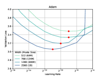
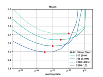
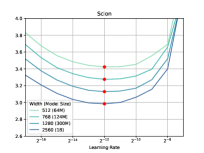
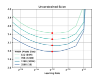
We build on the excellent modded-nanogpt codebase (Jordan et al., 2024a), which makes the following modernizations to Karpathy (2023): rotary embeddings is used instead of positional embeddings, RMS norm is used instead of LayerNorm, and linear decay schedule instead of a cosine stepsize. Scion and Unconstrained Scion use the (Sign Spectral Sign) configuration with scaling factors in accordance with Tables 3 and 4. We train for iterations with a batchsize of on the FineWeb dataset (see LABEL:tbl:hyperparams:nanoGPT regarding hyperparameters). In comparison with Adam, both Muon and (Unconstrained) Scion do not require learning rate warmup. We sweep over stepsizes and model width in Figure 1.
From Figure 1, we observe that the optimal stepsize of Scion and Unconstrained Scion transfer across model width as oppose to Adam and Muon. Even when the Muon optimizer is tuned on the largest model size it achieves a validation loss of 2.988 in comparison with 2.984 of Unconstrained Scion. Our methods completely remove the need for using Adam otherwise present in the Muon implementation, which permits an implementation that only requires storing one set of weights and one set of gradient (stored in half-precision) across all layers (see LABEL:app:impl). The experiments additionally demonstrates that our method works for weight sharing.
3B model
Using the optimal configuration of the 124M parameter proxy model, we perform a large model experiment on a 3B parameter model, which also increases the depth. Specifically, we take the embedding dimension to be 2560 and the depth to be 36. We observe in Table 5 that Unconstrained Scion outperforms all other methods. The loss curve is provided in LABEL:fig:NanoGPT:3B:loss-curve of LABEL:app:experiments.
| Adam | Muon | Unconstrained Scion | Scion |
|---|---|---|---|
| 3.024 | 2.909 | 2.882 | 2.890 |
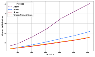
Large batches
To test the effect of large batches we fix the total number of tokens for the 124M parameter model, and sweep over the batch sizes while rescaling the total number of steps accordingly. The stepsize is optimized for each combination of batch size and optimizer. We observe that (Unconstrained) Scion is better at maintaining a low validation loss with increasing batch size than the baselines (cf., Figure 2).
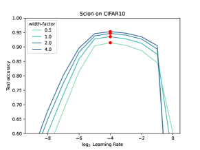
Image classification
We additionally test on a convolutional neural network (CNN) on the CIFAR10 dataset. We focus on Scion since norm control of the parameters is important for the setting. We use the configuration (Spectral Spectral Sign) and sweep over width and stepsize. The explicit control on the norm provided by Scion circumvents the need for the Frobenius norm normalization of the weights present in the base implementation (Jordan, 2024). The results are shown in Figure 3, which demonstrates the transferability of the optimal stepsize.
7 Acknowledgements
We thank Leena Chennuru Vankadara and Jeremy Bernstein for helpful discussion. This work was supported as part of the Swiss AI Initiative by a grant from the Swiss National Supercomputing Centre (CSCS) under project ID a06 on Alps. This work was supported by the Swiss National Science Foundation (SNSF) under grant number 200021_205011. This work was supported by Hasler Foundation Program: Hasler Responsible AI (project number 21043). Research was sponsored by the Army Research Office and was accomplished under Grant Number W911NF-24-1-0048. ASF was supported by a public grant from the Fondation Mathématique Jacques Hadamard.
References
- Arjevani et al. (2022) Arjevani, Y., Carmon, Y., Duchi, J. C., Foster, D. J., Srebro, N., and Woodworth, B. Lower bounds for non-convex stochastic optimization, 2022. URL https://arxiv.org/abs/1912.02365.
- Arjovsky et al. (2017) Arjovsky, M., Chintala, S., and Bottou, L. Wasserstein generative adversarial networks. In International conference on machine learning, pp. 214–223. PMLR, 2017.
- Balles et al. (2020) Balles, L., Pedregosa, F., and Roux, N. L. The geometry of sign gradient descent. arXiv preprint arXiv:2002.08056, 2020.
- Bartlett et al. (2017) Bartlett, P. L., Foster, D. J., and Telgarsky, M. J. Spectrally-normalized margin bounds for neural networks. In Guyon, I., Luxburg, U. V., Bengio, S., Wallach, H., Fergus, R., Vishwanathan, S., and Garnett, R. (eds.), Advances in Neural Information Processing Systems, volume 30. Curran Associates, Inc., 2017. URL https://proceedings.neurips.cc/paper_files/paper/2017/file/b22b257ad0519d4500539da3c8bcf4dd-Paper.pdf.
- Bauschke & Lucet (2012) Bauschke, H. and Lucet, Y. What is a Fenchel conjugate. Notices of the AMS, 59(1):44–46, 2012.
- Bernstein & Newhouse (2024a) Bernstein, J. and Newhouse, L. Modular duality in deep learning. arXiv preprint arXiv:2410.21265, 2024a.
- Bernstein & Newhouse (2024b) Bernstein, J. and Newhouse, L. Old optimizer, new norm: An anthology. arXiv preprint arXiv:2409.20325, 2024b.
- Bernstein et al. (2018) Bernstein, J., Wang, Y.-X., Azizzadenesheli, K., and Anandkumar, A. signSGD: Compressed optimisation for non-convex problems. In International Conference on Machine Learning, pp. 560–569. PMLR, 2018.
- Carlson et al. (2015a) Carlson, D., Cevher, V., and Carin, L. Stochastic spectral descent for restricted Boltzmann machines. In Artificial Intelligence and Statistics, pp. 111–119. PMLR, 2015a.
- Carlson et al. (2015b) Carlson, D., Hsieh, Y.-P., Collins, E., Carin, L., and Cevher, V. Stochastic spectral descent for discrete graphical models. IEEE Journal of Selected Topics in Signal Processing, 10(2):296–311, 2015b.
- Carlson et al. (2015c) Carlson, D. E., Collins, E., Hsieh, Y.-P., Carin, L., and Cevher, V. Preconditioned spectral descent for deep learning. Advances in neural information processing systems, 28, 2015c.
- Cisse et al. (2017) Cisse, M., Bojanowski, P., Grave, E., Dauphin, Y., and Usunier, N. Parseval networks: Improving robustness to adversarial examples. In International conference on machine learning, pp. 854–863. PMLR, 2017.
- Clarkson (2010) Clarkson, K. L. Coresets, sparse greedy approximation, and the frank-wolfe algorithm. ACM Trans. Algorithms, 6(4), September 2010. ISSN 1549-6325. doi: 10.1145/1824777.1824783. URL https://doi.org/10.1145/1824777.1824783.
- Conn et al. (2000) Conn, A. R., Gould, N. I., and Toint, P. L. Trust region methods. SIAM, 2000.
- Cutkosky & Mehta (2020) Cutkosky, A. and Mehta, H. Momentum improves normalized SGD. In International conference on machine learning, pp. 2260–2268. PMLR, 2020.
- Dahl et al. (2023) Dahl, G. E., Schneider, F., Nado, Z., Agarwal, N., Sastry, C. S., Hennig, P., Medapati, S., Eschenhagen, R., Kasimbeg, P., Suo, D., et al. Benchmarking neural network training algorithms. arXiv preprint arXiv:2306.07179, 2023.
- D’Angelo et al. (2023) D’Angelo, F., Andriushchenko, M., Varre, A., and Flammarion, N. Why do we need weight decay in modern deep learning? arXiv preprint arXiv:2310.04415, 2023.
- Duchi et al. (2011) Duchi, J., Hazan, E., and Singer, Y. Adaptive subgradient methods for online learning and stochastic optimization. Journal of Machine Learning Research, 12(61):2121–2159, 2011. URL http://jmlr.org/papers/v12/duchi11a.html.
- El Halabi (2018) El Halabi, M. Learning with structured sparsity: From discrete to convex and back. Technical report, EPFL, 2018.
- Frank et al. (1956) Frank, M., Wolfe, P., et al. An algorithm for quadratic programming. Naval research logistics quarterly, 3(1-2):95–110, 1956.
- Gupta et al. (2017) Gupta, V., Koren, T., and Singer, Y. A unified approach to adaptive regularization in online and stochastic optimization. arXiv preprint arXiv:1706.06569, 2017.
- Hazan et al. (2015) Hazan, E., Levy, K., and Shalev-Shwartz, S. Beyond convexity: Stochastic quasi-convex optimization. Advances in neural information processing systems, 28, 2015.
- He et al. (2015) He, K., Zhang, X., Ren, S., and Sun, J. Delving deep into rectifiers: Surpassing human-level performance on imagenet classification. In Proceedings of the IEEE international conference on computer vision, pp. 1026–1034, 2015.
- Hinton et al. (2012) Hinton, G., Srivastava, N., and Swersky, K. Neural networks for machine learning lecture 6a overview of mini-batch gradient descent. Cited on, 14(8):2, 2012.
- Jaggi (2013) Jaggi, M. Revisiting Frank-Wolfe: Projection-free sparse convex optimization. In International conference on machine learning, pp. 427–435. PMLR, 2013.
- Jordan (2024) Jordan, K. Cifar-10 airbench, 2024. URL https://github.com/KellerJordan/cifar10-airbench.
- Jordan et al. (2024a) Jordan, K., Bernstein, J., Rappazzo, B., @fernbear.bsky.social, Vlado, B., Jiacheng, Y., Cesista, F., Koszarsky, B., and @Grad62304977. modded-nanogpt: Speedrunning the nanogpt baseline, 2024a. URL https://github.com/KellerJordan/modded-nanogpt.
- Jordan et al. (2024b) Jordan, K., Jin, Y., Boza, V., Jiacheng, Y., Cecista, F., Newhouse, L., and Bernstein, J. Muon: An optimizer for hidden layers in neural networks, 2024b. URL https://kellerjordan.github.io/posts/muon/.
- Karpathy (2023) Karpathy, A. nanoGPT. https://github.com/karpathy/nanoGPT, 2023. Accessed: 2025-01-25.
- Karras et al. (2024) Karras, T., Aittala, M., Lehtinen, J., Hellsten, J., Aila, T., and Laine, S. Analyzing and improving the training dynamics of diffusion models. In Proceedings of the IEEE/CVF Conference on Computer Vision and Pattern Recognition, pp. 24174–24184, 2024.
- Kelner et al. (2014) Kelner, J. A., Lee, Y. T., Orecchia, L., and Sidford, A. An almost-linear-time algorithm for approximate max flow in undirected graphs, and its multicommodity generalizations. In Proceedings of the twenty-fifth annual ACM-SIAM symposium on Discrete algorithms, pp. 217–226. SIAM, 2014.
- Kingma (2014) Kingma, D. P. Adam: A method for stochastic optimization. arXiv preprint arXiv:1412.6980, 2014.
- Lange (2016) Lange, K. MM optimization algorithms. SIAM, 2016.
- Large et al. (2024) Large, T., Liu, Y., Huh, M., Bahng, H., Isola, P., and Bernstein, J. Scalable optimization in the modular norm. arXiv preprint arXiv:2405.14813, 2024.
- Lu et al. (2022) Lu, M., Luo, X., Chen, T., Chen, W., Liu, D., and Wang, Z. Learning pruning-friendly networks via Frank-Wolfe: One-shot, any-sparsity, and no retraining. In International Conference on Learning Representations, 2022.
- McMahan & Streeter (2010) McMahan, H. B. and Streeter, M. Adaptive bound optimization for online convex optimization, 2010. URL https://arxiv.org/abs/1002.4908.
- Miyato et al. (2018) Miyato, T., Kataoka, T., Koyama, M., and Yoshida, Y. Spectral normalization for generative adversarial networks. arXiv preprint arXiv:1802.05957, 2018.
- Mokhtari et al. (2020) Mokhtari, A., Hassani, H., and Karbasi, A. Stochastic conditional gradient methods: From convex minimization to submodular maximization. Journal of machine learning research, 21(105):1–49, 2020.
- Nesterov (2012) Nesterov, Y. Efficiency of coordinate descent methods on huge-scale optimization problems. SIAM Journal on Optimization, 22(2):341–362, 2012.
- Pethick et al. (2025) Pethick, T., Raman, P., Minorics, L., Hong, M., Sabach, S., and Cevher, V. sam: Memory-efficient sharpness-aware minimization via nuclear norm constraints. Transactions on Machine Learning Research, 2025.
- Pokutta et al. (2020) Pokutta, S., Spiegel, C., and Zimmer, M. Deep neural network training with Frank-Wolfe. arXiv preprint arXiv:2010.07243, 2020.
- Saxe et al. (2013) Saxe, A. M., McClelland, J. L., and Ganguli, S. Exact solutions to the nonlinear dynamics of learning in deep linear neural networks. arXiv preprint arXiv:1312.6120, 2013.
- Vershynin (2018) Vershynin, R. High-dimensional probability: An introduction with applications in data science, volume 47. Cambridge university press, 2018.
- Vondrák (2008) Vondrák, J. Optimal approximation for the submodular welfare problem in the value oracle model. In Proceedings of the fortieth annual ACM symposium on Theory of computing, pp. 67–74, 2008.
- Wright (2006) Wright, S. J. Numerical optimization, 2006.
- Xie & Li (2024) Xie, S. and Li, Z. Implicit bias of AdamW: norm constrained optimization. arXiv preprint arXiv:2404.04454, 2024.
- Yang & Hu (2021) Yang, G. and Hu, E. J. Tensor programs iv: Feature learning in infinite-width neural networks. In International Conference on Machine Learning, pp. 11727–11737. PMLR, 2021.
- Yang et al. (2022) Yang, G., Hu, E. J., Babuschkin, I., Sidor, S., Liu, X., Farhi, D., Ryder, N., Pachocki, J., Chen, W., and Gao, J. Tensor programs v: Tuning large neural networks via zero-shot hyperparameter transfer. arXiv preprint arXiv:2203.03466, 2022.
- Yang et al. (2023) Yang, G., Simon, J. B., and Bernstein, J. A spectral condition for feature learning. arXiv preprint arXiv:2310.17813, 2023.
- You et al. (2017) You, Y., Gitman, I., and Ginsburg, B. Large batch training of convolutional networks. arXiv preprint arXiv:1708.03888, 2017.
- You et al. (2019) You, Y., Li, J., Reddi, S., Hseu, J., Kumar, S., Bhojanapalli, S., Song, X., Demmel, J., Keutzer, K., and Hsieh, C.-J. Large batch optimization for deep learning: Training bert in 76 minutes. arXiv preprint arXiv:1904.00962, 2019.
- Zamani & Glineur (2023) Zamani, M. and Glineur, F. Exact convergence rate of the last iterate in subgradient methods. arXiv preprint arXiv:2307.11134, 2023.
- Zhao et al. (2020) Zhao, S.-Y., Xie, Y.-P., and Li, W.-J. Stochastic normalized gradient descent with momentum for large batch training. arXiv preprint arXiv:2007.13985, 2020.
Appendix
.tocmtappendix \etocsettagdepthmtchapternone \etocsettagdepthmtappendixsubsection