NatureLM: Deciphering the Language of Nature for Scientific Discovery

Abstract

Foundation models have revolutionized natural language processing and artificial intelligence, significantly enhancing how machines comprehend and generate human languages. Inspired by the success of these foundation models, researchers have developed foundation models for individual scientific domains, including small molecules, materials, proteins, DNA, and RNA. However, these models are typically trained in isolation, lacking the ability to integrate across different scientific domains. Recognizing that entities within these domains can all be represented as sequences, which together form the “language of nature”, we introduce Nature Language Model (briefly, NatureLM), a sequence-based science foundation model designed for scientific discovery. Pre-trained with data from multiple scientific domains, NatureLM offers a unified, versatile model that enables various applications including: (i) generating and optimizing small molecules, proteins, RNA, and materials using text instructions; (ii) cross-domain generation/design, such as protein-to-molecule and protein-to-RNA generation; and (iii) achieving state-of-the-art performance in tasks like SMILES-to-IUPAC translation and retrosynthesis on USPTO-50k.

NatureLM offers a promising generalist approach for various scientific tasks, including drug discovery (hit generation/optimization, ADMET optimization, synthesis), novel material design, and the development of therapeutic proteins or nucleotides. We have developed NatureLM models in different sizes (1 billion, 8 billion, and 46.7 billion parameters) and observed a clear improvement in performance as the model size increases.

1 Introduction

Foundation models, including the GPT brown2020languagemodelsfewshotlearners ; gpt4technicalreport ; openai2024gpt4ocard , Gemini geminiteam2024geminifamilyhighlycapable ; geminiteam2024gemini15unlockingmultimodal , Phi abdin2024phi3technicalreporthighly ; phi4report , Llama dubey2024llama3herdmodels , Mistral jiang2023mistral7b ; jiang2024mixtralexperts , DeepSeek deepseekv3 ; deepseekai2025r1 , and Qwen yang2024qwen2technicalreport ; qwen2025qwen25technicalreport , represent a transformative advancement in artificial intelligence. These models, trained on massive web-scale datasets, are designed to serve as general-purpose tools, capable of handling a wide range of tasks with a single architecture. The most notable capabilities of foundation models include their abilities to perform tasks without fine-tuning, a phenomenon known as zero-shot learning, and their few-shot learning abilities which allow them to adapt to new tasks by drawing inferences from just a few examples.

Despite their success in general-purpose tasks, early investigations ai4science2023impactlargelanguagemodels highlight significant room for improvement for scientific tasks involving small molecules, proteins, DNA, RNA, or materials. In particular, foundation models struggle with precise quantitative predictions (e.g., ligand-protein binding affinity, protein-protein interactions, DNA properties) ai4science2023impactlargelanguagemodels and rational design and optimization of compounds, proteins, and materials. Moreover, ensuring the scientific accuracy of outputs from these models remains as a grand challenge.

Recently, there has been a concerted effort to develop large-scale foundation models specifically tailored for scientific tasks. These approaches can be broadly divided into four categories:

1. Domain-specific foundation models. These models, such as ProGen ProGen and ESM3 esm3 for proteins, DNABERT zhou2024dnabert2 and Evo evo2024science for DNA sequences, scGPT Cui2024scgpt for single-cell data, and chemical language models liu2023molxpt ; segler2018generating for small molecules, are trained specifically on token sequence representations for individual scientific domains.

2. Fine-tuned general-purpose models. This approach adapts well-trained large language models for specific scientific domains, as demonstrated by Tx-LLM chaves2024tx for small molecules and ProLLAMA lv2024prollamaproteinlanguagemodel for proteins.

3. Scientific data enhanced large language models (LLMs). This approach BioGPT2022Luo ; liu2023molxpt ; galactica2022 trains LLMs from scratch mainly with text data and a small portion of scientific data.

4. Integration of specific scientific modules. In this approach, external modules, such as pre-trained molecular or protein encoders, are integrated into general-purpose models (e.g., Llama) via lightweight adapters drugchat ; proteinchat .

While these approaches have made considerable progress, they do face notable limitations. Domain-specific models (approach #1) are restricted to their respective fields, limiting their ability to capture interdisciplinary insights for cross-domain applications. Fine-tuning general-purpose models (approach #2) and scientific data enhanced LLMs (approach #3) show promise but are often constrained by small-scale scientific datasets, e.g., around 90% text data and only 10% scientific data in galactica2022 , which hinders the models’ capacity to capture the complexity of scientific tasks. The integration of external modules (approach #4) faces challenges in aligning inputs effectively with large language models, and most implementations opt for limited fine-tuning with small datasets, leaving the core models largely unchanged.

The existence of these limitations emphasizes the necessity for a science foundation model, to fulfill the sophisticated demands of scientific research. A model of this kind must not only be highly proficient in producing precise scientific predictions but also adept at designing and optimizing scientific entities conditioned on context information. A perfect science foundation model ought to have the capacity to handle a diverse range of inputs. These inputs can span from literature text, to scientific sequence data such as protein or DNA sequences, and further to structural data like 3D protein/DNA structures and their dynamic behaviors. In the present study, our focus is on sequence-based data for representing biological, chemical, material systems, and natural language:

• DNA, RNA, and proteins, which are often referred to as the “language of nature”, are intrinsically represented by sequences. Additionally, many other scientific entities like small molecules and materials can be effectively represented as sequences through well-established domain-specific techniques Weininger1988 .

• Sequence data is highly compatible with the current mainstream large language models (LLMs). Through the continuous pre-training of LLMs, we are able to utilize the scientific knowledge embedded in these general-purpose LLMs to tackle complex scientific challenges.

• Sequential data provides remarkable flexibility when combined with autoregressive paradigms bond2021deep ; yenduri2024gpt . These paradigms, which are extensively employed in generative models, are capable of effectively modeling the highly complex distributions of any scientific object that can be presented in the form of a sequence.

We introduce Nature Language Model (briefly, NatureLM), a sequence-based science foundation model tailored for scientific tasks. NatureLM is designed to handle the complexity of small molecules, proteins, DNA, RNA, materials, and their associated textual information. NatureLM follows the Transformer decoder architecture and is trained on a corpus of 143 billion tokens collected from various scientific domains. Our experiments demonstrate that NatureLM significantly outperforms general-purpose foundation models for scientific tasks. Specifically, NatureLM excels in tasks such as:

1. Following textual instructions to generate/design and optimize scientific molecular entities.

2. Performing cross-domain generation tasks, such as designing small molecules or RNA binders for proteins as well as designing guide RNA sequences given a DNA template for CRISPR systems.

3. Achieving state-of-the-art performance in retrosynthesis and SMILES-to-IUPAC translation.

To investigate the scalability of NatureLM with respect to model size, we trained three versions of NatureLM with varying parameter configurations. As illustrated in Fig. 1, among the 22 categories of tasks evaluated, 18 categories exhibited clear improvements with increasing model size (i.e., 8x7B demonstrated the best performance, followed by 8B, and then 1B), underscoring the potential of large foundation models for scientific discovery. Additionally, we demonstrate the efficacy of reinforcement learning in enhancing the post-training performance of NatureLM for molecular property optimization and dedicated finetuning for retrosynthesis.

Figure 1: The overall ranking of models of varying sizes is depicted in the chart. The blue, orange, and green bars correspond to the results for the small (1B), medium (8B), and large (8x7B) models, respectively. A better rank is indicated by the “outsider” bar. The 8x7B model achieves top performance in 19 tasks, while the 8B model excels in 3 tasks. 18 categories exhibited performance improvements with increasing model size (i.e., 8x7B demonstrated the best performance, followed by 8B, and then 1B), highlighting the potential of large foundation models for scientific applications.

In summary, our development of the NatureLM represents a significant step towards building a generalist model across multiple scientific domains. By harnessing the capabilities of text-based instructions, NatureLM serves as a powerful tool for scientific discovery, enabling cross-domain generation and optimization in areas such as drug discovery, materials science, and the development of therapeutic proteins and nucleotides. Ideally, a foundation model should support a broad range of tasks while demonstrating strong zero-shot and few-shot capabilities. NatureLM shows great promise, but its language capabilities and few-shot learning skills still lag behind leading large language models. We will address these limitations in future iterations, positioning NatureLM as a key player in the continued evolution of scientific foundation models.

2 Method

2.1 Pre-training data

The pre-training data includes text, small molecules, proteins, materials, DNA, and RNA, all in the format of sequences:

1. Small molecules are converted into Simplified Molecular Input Line Entry System (SMILES) notations, obtained by applying depth-first search algorithm on molecular graphs to yield a linear representation of the chemical structure Weininger1988 . The SMILES are tokenized by the commonly used regular expression for molecules.

2. Proteins, DNA and RNA are depicted using FASTA format, which sequentially lists the amino acids or nucleotides. The sequences are tokenized into individual units, with proteins broken down into their constituent amino acids and DNA/RNA into their respective nucleotides.

3. For crystal material data, both the chemical composition and the associated space group number are flattened into a sequence. For example, consider the material from the material project with ID mp-1960, as shown in Fig. 2. This material has 12 atoms in its cell, consisting of 4 Li and 8 O atoms. We flatten this information as depicted in the figure. The space group is Fm3m, which corresponds to the International Space Group Number 225, and we represent it with $\langle$sg$\cdots$$\rangle$.

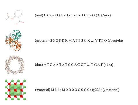
Figure 2: Example data from each domain. The small molecule is Aspirin (PubChem CID: 2244) and visualized by RDKit greg_landrum_2025_14779836 . The protein snapshot is from the PDB bank with ID 7CAM Wang2020-vw . The DNA structure is split into chain I and chain J from PDB 1KX5 Davey2002im and visualized by UCSF Chimera chimera2004software . The material snapshot is from the material project with ID mp-1960 osti_1194803 .

An example of the data is in Fig. 2. The vocabulary sizes of small molecules, proteins, material, DNA and RNA are 1401, 26, 396, 16 and 16 respectively. To differentiate scientific entities from regular text, each scientific sequence is enclosed by a pair of special tokens: $\langle$mol$\rangle$$\cdots$$\langle$/mol$\rangle$ for small molecules, $\langle$protein$\rangle$$\cdots$$\langle$/protein$\rangle$ for proteins, $\langle$material$\rangle$$\cdots$$\langle$/material$\rangle$ for materials, $\langle$dna$\rangle$$\cdots$$\langle$/dna$\rangle$ for DNA and $\langle$rna$\rangle$$\cdots$$\langle$/rna$\rangle$ for RNA. Specifically, we use $\langle$product$\rangle$$\cdots$$\langle$/product$\rangle$ and $\langle$reactant$\rangle$$\cdots$$\langle$/reactant$\rangle$ to represent products and reactants for small molecules in chemical reactions. We use $\langle$antibody$\rangle$$\cdots$$\langle$/antibody$\rangle$ to denote antibodies. For example, benzene is represented by $\langle$mol$\rangle$c1ccccc1$\langle$/mol$\rangle$. More examples can be found within the following sections.

The pre-training data contains single-domain sequences and cross-domain sequences. A single-domain sequence comes from one domain, such as pure text sequences, SMILES sequences for small molecules, and FASTA sequences for proteins. A cross-domain sequence includes data from two different domains, building connections across domains. The distribution of our pre-training data is visualized in Fig. 3 and more details are left in Table S1.

Figure 3: Distribution of the pre-training data, measured by the number of tokens of each category.

Our cross-domain data is organized into three categories.

1. Interleaved Sequences: Inspired by liu2023molxpt , we process scientific literature by initially employing a named entity recognition tool, BERN2 bern2 , to identify the mentions of small molecules and proteins within the corpus. These entities are then converted into their corresponding SMILES and FASTA sequences. Consequently, the small molecules and proteins are wrapped by text, creating an interleaved data structure that bridges the gap between textual information and scientific data. We also develop a quality filter to remove low-quality sentences. This formulation is also similar to the one that has been used in multi-modal LLMs where image tokens are wrapped inside text Zhu2023MultimodalCA ; Zhan2024AnyGPTUM ; team2024chameleon . We provide an example of interleaved sequences.

   Example 2.1.

   A prospective, randomized clinical trial was performed to study the efficacy of povidone iodine $\langle$mol$\rangle$C=CN1CCCC1=O.II$\langle$/mol$\rangle$ ( Betadine $\langle$mol$\rangle$C=CN1CCCC1=O.II$\langle$/mol$\rangle$) suppositories for the treatment of bacterial vaginosis (BV) in comparison to capsules containing lactobacilli (Dderlein Med).

2. Parallel Text and Scientific Entities: Leveraging databases such as PubChem, UniProt, and NCBI, we extract descriptive information about specific proteins and small molecules. Additionally, from the Materials Project website, material-related data such as bandgap, energy above hull, and other properties are gathered and translated into textual descriptions. This process results in parallel datasets that align scientific facts with their textual counterparts, enhancing the richness of the information.

3. Linking DNA with Proteins Through the Central Dogma: For DNA sequences, we identify segments that can be transcribed and translated into proteins, following the central dogma of molecular biology. These identified DNA segments are then replaced with the equivalent protein sequences, establishing a direct connection between the genetic blueprint and its functional protein products. This method not only reflects the biological process but also creates a dataset that encapsulates the relationship between nucleotide and amino acid sequences.

	Samples	Tokens	Samples	Tokens
	(by million)	(by billion)	(%)	(%)
Interleaved Sequence	4.3	4.0	10.2	31.3
Text-SMILES	33.0	3.0	78.8	24.0
Text-protein	1.9	1.4	4.6	10.8
Text-material	1.7	0.2	4.0	1.6
DNA-protein	1.0	4.1	2.4	32.3
Total	41.9	12.7	100	100

Table 1: Statistics of cross-domain data.

The statistics of cross-domain data is in Table 1. Both interleaved sequences and text-science parallel data are types of cross-domain data that aim to facilitate cross-domain interaction. For interleaved sequences, the sources are literature, which can cover a broader range of general topics and wider domains. In contrast, parallel data sources are existing databases that focus on specific properties. Although the topics covered by parallel data are not as diverse as those in interleaved sequences, the amount of data available for each given property is greater. These distinctions highlight the complementary nature of the two types of cross-domain data.

2.2 Post-training data

We curated a dataset for post-training with about 5.1 million instruction-response pairs encompassing six domains, small molecules, proteins, materials, DNA, RNA and general text (Figure 4). The dataset includes over 60 sub-tasks. For each sub-task, multiple prompts were manually crafted to form diverse instruction-response pairs, covering essential scientific tasks such as molecular optimization, antibody design, and guide RNA design. We provide two examples below:

Example 2.2.

$\rhd$ Example 1:

Instruction:
Create a guiding RNA to interact with the DNA sequence
$\langle$dna$\rangle$CCCAGAGC$\cdots$GGGCCTGTC$\langle$/dna$\rangle$.
Response:$\langle$rna$\rangle$AGGGGACAAACCTTCATCCA$\langle$/rna$\rangle$

$\rhd$ Example 2

Instruction:
What product could potentially form from the reaction of the given reactants? $\langle$product$\rangle$C([C@H]1N(c2c(C(N[C@@H](CC)c3ccccc3)=O)c3c(nc2-c2ccccc2)cccc3)CCC1)(=O)OC$\langle$/product$\rangle$
Response:
$\langle$reactant$\rangle$C([C@H]1N(c2c(C(N[C@@H](CC)c3ccccc3)=O)c3c(nc2-c2ccccc2)cccc3)CCC1)O$\langle$/reactant$\rangle$

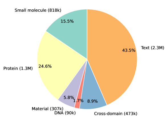
Figure 4: Statistics of post-training data, measured by the number of sequences.

The text data were sourced from open-source instruction tuning datasets like OIG , aiming to ensure that the model not only excels in scientific tasks but also maintains general language capabilities.

2.3 Model architecture

NatureLM models are built upon well-trained large language models (LLMs) with some additional parameters for newly introduce scientific tokens. We used Llama 3 8B dubey2024llama3herdmodels and Mixtral 8x7B jiang2024mixtralexperts to initialize the main part of NatureLM and continued pre-training using the science data described in Section 2.1. Additionally, we trained a model with 1B parameters, which replicates the structural design of Llama 3 but with a reduced number of layers and smaller hidden dimensions. Its pre-training begins with a random selection of 300 billion pure text tokens from the SlimPajama dataset cerebras2023slimpajama , followed by the science data we collected in Section 2.1. This approach ensures a consistent training methodology across all three models. The details of the model architecture are provided in Table 2.

Model Parameters	1B	8B	8x7B
Hidden Dimensions	2048	4096	4096
FFN Dimensions	5504	14336	14336
Attention Heads	32	32	32
KV Heads	8	8	32
Number of Layers	16	32	32
Vocabulary Size	130,239	130,239	38,078

Table 2: Model parameters of different sizes of NatureLM.

2.4 Continued pre-training

To address the intricate comprehension required for scientific tasks, NatureLM introduces specific tokens for scientific entities. Consequently, we augment the vocabulary of the chosen LLMs. The embedding weights for these newly introduced tokens are randomly initialized. Directly tuning from pre-training usually causes instability and potentially compromises the language capabilities of the original LLMs. This is primarily due to the introduction of new tokens and the mismatch between the well-trained text tokens and randomly initialized scientific tokens.

To circumvent this issue, we have devised a two-stage pre-training procedure:

Stage 1: Training is exclusively concentrated on the newly introduced tokens. During this phase, the parameters of the existing model are frozen. This allows the new tokens to adapt to the model gradually, mitigating the risk of instability.

Stage 2: Once the new tokens are adequately trained, we proceed to the second phase where the entire network, including both new and existing parameters, is trained. This joint optimization process ensures that the new tokens are seamlessly integrated with the existing ones, enhancing the model’s overall performance.

This two-stage training approach not only fosters a thorough understanding of the scientific domain but also preserves the integrity and robustness of the underlying language model by preventing potential instabilities. The detailed training recipe is summarized in Table S2.

The validation loss for the three versions of the models is illustrated in Fig. 5. All validation losses decrease as the model size increases from 1 billion to 8 billion, and 8x7 billion. This indicates that larger models are better at capturing the underlying patterns in the data, which is expected due to their increased capacity. The most significant decreases are observed in the text and protein data, suggesting that these datasets benefit more from larger models.

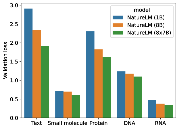
Figure 5: Validation loss for the 1B, 8B, and 8x7B models of NatureLM. Larger models result in smaller validation losses across each domain. NatureLM (8B) is short for “Llama 3 8B NatureLM” throughout this paper.

2.5 Post-training

In the post-training phase, we mainly employ supervised fine-tuning (SFT) using the instruction-response pair data outlined in Section 2.2. These pairs are structured into sequences utilizing the template “Instruction: {instruction}\n\n\nResponse: {response}” where “{instruction}” and “{response}” serve as placeholders. During the model optimization, the training loss is computed solely on the response part of the sequence. Unlike in the pre-training phase, each sequence contains a single instruction-response pair rather than multiple pairs packed into one sequence. Empirical evidence suggests that this approach aids in stabilizing the post-training process. The 1B and 8B models are trained for 20k steps, while the 8x7B model is trained for 7.8k steps (due to resource constraint). We also explore using RLHF after supervised finetuning and results are discussed in Section 8.1.

2.6 Inference acceleration

As NatureLM will be tested on many downstream tasks, we need to accelerate inference speed to save computational cost. We adopted the following approaches: (1) PagedAttention pagedattention , which optimizes LLM serving by partitioning the key-value (KV) cache into fixed-size, non-contiguous blocks, reducing memory fragmentation and enabling efficient memory sharing; and (2) Selective Batching orca , which batches compatible operations while handling attention separately, allowing for flexible and efficient processing of requests with varying input lengths. We employed the vLLM framework vllm2024 to serve NatureLM models, leveraging its implementations of both PagedAttention and Selective Batching. These optimizations were applied to the 1B, 8B, and 8×7B models. Consequently, the inference speed for the NatureLM 8×7B model reached approximately 525 tokens per second with Brain Float 16 (BF16) precision on two NVIDIA A100 GPUs.

3 Small molecule tasks

We assess the capabilities of NatureLM in terms of small molecule generation from the following perspectives:

1. The unconditional generation ability (Section 3.1);

2. The basic properties (such as QED, TSPA, etc.) to small molecule generation (Section 3.2);

3. The translation between small molecule SMILES and IUPAC (Section 3.3);

4. Utilize NatureLM to aid the drug discovery pipeline, which encompasses the generation and optimization of hit compounds (Section 3.4), optimization of binding affinity (Section 3.5), ADMET optimization (Section 3.6), and the synthesis routes of the compounds (Section 3.7).

3.1 Unconditional molecular generation

We input the special token $\langle$mol$\rangle$ to NatureLM and let the model generate SMILES. The generation process stops upon encountering the special token $\langle$/mol$\rangle$. We assess the validity of the generated SMILES by checking if they can be converted into molecules using RDKit. Additionally, we evaluate the uniqueness of the valid SMILES by calculating the ratio of unique valid SMILES to the total valid SMILES.

The evaluation results are presented in Table 3. The results demonstrate a clear trend: as the model size increases, the performance in terms of validity improves. NatureLM exhibits a consistent increase in uniqueness as the model’s capacity grows. We also establish comparisons between NatureLM and three generalist models: Llama 3 (8B), Mixtral (8x7B), and GPT-4. Our NatureLM significantly outperforms the others in terms of uniqueness. As for validity, the results show that GPT-4 demonstrates a remarkable ability to generalize chemically valid SMILES.

	Validity (%)	Unique (%)
Llama 3 (8B)	77.9	35.1
Mixtral (8x7B)	72.6	35.1
GPT-4	99.6	54.6
NatureLM (1B)	94.9	91.1
NatureLM (8B)	96.8	96.6
NatureLM (8x7B)	98.8	98.8

Table 3: Unconditional evaluation of small molecules generation.

3.2 Property-to-molecule generation

The task is to generate molecules with specified properties, which is a critical aspect of molecular design. An example is shown as follows:

Example 3.1.

Instruction:
Generate a molecule with four hydrogen bond donors.
Response:
$\langle$mol$\rangle$C(C[C@@H](C(=O)O)N)CN=C(N)N$\langle$/mol$\rangle$

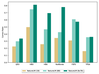
Figure S1: Correct ratio of property-to-molecule generation. We treat the generated molecule as a correct one if $\lvert v^{\prime}-v\lvert\leq\delta$, where $v^{\prime}$ is its property value and $v$ is the input value. $\delta$ is set to 0 for HBA, HBD, RotBonds, 0.05 for QED and FSP3, and 5 for TPSA.

We conduct evaluations of NatureLM on six distinct properties: Quantitative Estimate of Drug-likeness (QED), hydrogen bond acceptors (HBA), hydrogen bond donors (HBD), fraction of sp3 hybridized carbons (FSP3), rotatable bonds (RotBonds), and topological polar surface area (TPSA). All these properties can be calculated using RDKit. For each property, we select multiple values as inputs to the model (see Table S3). We generate 100 molecules for each input and evaluate them with metrics including the Spearman correlation (Fig. 6a) and the correct ratio (Fig. S1). Our findings reveal that on certain property, such as TPSA, the model demonstrates a Spearman correlation greater than 0.8, illustrating the consistency between the generated molecules and the input specifications (Fig. 6b).

Additionally, our model can handle the combination of multiple properties. For example, when given the command “Generate a compound with QED 0.5 and TPSA 40”, the model generates compounds that meet both specified criteria. The results are shown in Fig. 6c. The majority of the generated compounds have QED and TPSA values centered around our desired properties (i.e., 0.5 and 40), demonstrating the versatility and effectiveness of NatureLM in multi-property molecular generation.

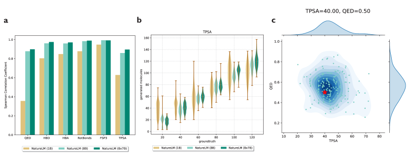
Figure 6: Evaluation of property-to-molecule generation. (a) Bar plot of the Spearman correlation coefficients between the input property values and generated molecules’ property values. (b) Violin plot showing the input TPSA values and generated molecules’ TPSA values. More properties are left in Fig. LABEL:fig:basic_to_cmpd_violinplot. (c) The joint distribtion of the generated molecules’ TPSA and QED given the input “TPSA=40, QED=0.5” (see Fig. LABEL:fig:qed_fsp3_joint_optim for more cases).

3.3 Translation between SMILES and IUPAC

We evaluate NatureLM on the translation between SMILES and IUPAC on NC-I2S and NC-S2I yu2024llasmol , the bidirectional IUPAC-SMILES translation dataset comprising 2993 pairs of SMILES and their corresponding IUPAC names (Table 4). We ensure that there is no test set leakage in this setting. On both text-to-SMILES and SMILES-to-text translation tasks, NatureLM (8x7B) outperforms all competing language models in terms of accuracy, demonstrating our model’s strong learning capability for text-molecule correspondence. NatureLM significantly outperforms GPT-4 and Claude 3 Opus claude3 , strong generalist large language models (LLMs), highlighting the necessity of training on scientific data. Compared with another LLM trained on text and SMILES corpus LlaSMol_Mistral yu2024llasmol , NatureLM also obtains significantly better performance. Moreover, NatureLM (8x7B) performs comparably with STOUT rajan2024stout , the widely-used model trained specially for IUPAC-SMILES translation task, demonstrating NatureLM’s potential as a scientific generalist in specific domains. The performance increases from NatureLM (1B) to NatureLM (8x7B), exhibiting the scaling benefits of larger models.

	IUPAC-to-SMILES	SMILES-to-IUPAC
STOUT	0.735	0.565
GPT-4	0.033	0
Claude 3 Opus	0.177	0
LlaSMolMistral	0.701	0.290
NatureLM (1B)	0.476	0.284
NatureLM (8B)	0.679	0.517
NatureLM (8x7B)	0.704	0.607

Table 4: IUPAC-SMILES translation results. Models are evaluated by top-5 accuracy.

3.4 Target-aware hit generation and optimization

The task is to generate small molecule compounds given the target protein sequence. The combination of NatureLM and structure-based compound design will be explored in the future. We test NatureLM within two distinct scenarios:

(1) Generate compounds from the target protein sequences. This process is crucial for the hit identification stage of drug discovery, with the goal of discovering chemical entities that exhibit specific interactions with the target protein.

(2) Generate molecular fragments based on the target protein sequences and partial molecular structures as inputs. This method is instrumental during the lead optimization phase, where we scrutinize and refine the molecular architecture to amplify efficacy and precision.

The examples are shown below:

Example 3.2.

$\rhd$Scenario 1: Complete molecule generation

Instruction:
Produce a compound guided by the target
$\langle$protein$\rangle$LALSLTADQMVSALL…SYDLLLEMLDAH$\langle$/protein$\rangle$
Response:$\langle$mol$\rangle$CC1=C(c2cccc(O)c2)C(c2ccc(I)cc2)Oc2ccc(O)cc21$\langle$/mol$\rangle$

$\rhd$Scenario 2: Fragment generation

Instruction:
Design a compound with reference to the target
$\langle$protein$\rangle$DTKEQRILR$\cdots$EKAIYQGP$\langle$/protein$\rangle$ and the fragment $\langle$fragA$\rangle$O=c1[nH]cnc2c(O)cc([*:1])c([*:2])c12$\langle$/fragA$\rangle$
Response:
$\langle$fragB$\rangle$Fc1ccc([*:1])cc1.Fc1ccc([*:2])cc1$\langle$/fragB$\rangle$

Here, “[*:digit]” refers to the connection point of the molecular fragment, like the R1 and R2 in Fig. 7.

In the first scenario, we compare NatureLM with a sequence generation method, TamGen TamGen , and two approaches that design compounds in 3D space based on the input target: a diffusion-based method, TargetDiff targetdiff , and an autoregressive generation method in 3D space, Pocket2Mol pocket2mol . We follow the evaluation procedure outlined in the TamGen paper TamGen , which includes calculating the docking score using AutoDock Vina, as well as assessing the QED, synthetic accessibility scores (SAS), diversity of the generated compounds, the percentage of compounds with logP in the range [0,5], and the percentage of compounds satisfying the rule-of-five. The results are presented in Table 5. We can see that in terms of docking score, QED and synthesis ability, NatureLM surpasses previous baselines, highlighting its effectiveness.

	Vina	QED	SAS	Diversity	LogP$\in[0,5]$	Ro5
Pocket2Mol	-4.90	0.52	0.84	0.87	0.76	1
TargetDiff	-6.08	0.55	0.67	0.83	0.74	0.98
TamGen	-6.66	0.56	0.76	0.75	0.84	0.99
NatureLM (1B)	-6.80	0.64	0.82	0.77	0.85	0.99
NatureLM (8B)	-6.92	0.62	0.81	0.73	0.84	0.99
NatureLM (8x7B)	-6.95	0.62	0.82	0.75	0.84	0.99

Table 5: Statistics of target to complete compound sequence generation.

Additionally, we utilize NatureLM for fragment generation. We selected three papers published after May 2024 Tangallapally2024pdb6PE6 ; Tarr2024pdb9BCG ; Mammoliti2024pdb3xln , where part of their task is to solve the issue of compound optimization. In this context, the input includes a target protein and a backbone that needs optimization. The results are illustrated in Fig. 7. In this instance, it is evident that larger models typically yield superior docking scores.

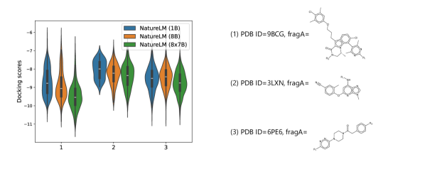
Figure 7: Violin plot of docking scores for molecules in target-to-fragment generation. This violin plot presents the docking scores of molecules involved in target-to-fragment generation. We selected three recent papers that focus on fragment optimization: Tarr2024pdb9BCG , Mammoliti2024pdb3xln and Tangallapally2024pdb6PE6 , which utilize PDB IDs 9BCG, 3LXN, and 6PE6, respectively. The input fragment is visualized alongside its corresponding PDB ID for clarity.

3.5 Text-guided binding affinity optimization

To further improve the binding affinity between a target and a molecule, we propose a text-guided binding affinity optimization task. Given a target name and a molecule with a known binding affinity for that target, we aim to generate molecules with higher binding affinity, which is crucial for lead optimization. An example is shown below:

Example 3.3.

Instruction:
Improve the binding affinity on Uridine-cytidine kinase 2 of $\langle$mol$\rangle$Cc1ccc(-c2nc3c(c(SCC(=O)Nc4ccccc4)n2)Cc2cccc(C)c2O3)cc1$\langle$/mol$\rangle$
Response:
$\langle$mol$\rangle$Cc1ccc(-c2nc3c(c(SCC(=O)Nc4cccc(C(=O)O)c4)n2)Cc2cccc(C) c2O3)cc1$\langle$/mol$\rangle$

Here, the target information is provided in text format, which complements the FASTA representation used in Section 3.4. We will combine them in the future.

We test NatureLM on 12 targets that are not present in the post-training data and use a hybrid retrieval and docking approach for evaluation. Specifically, for the generated molecules, if we can retrieve their binding affinity values from the ChEMBL database, we compare these values with the original molecule’s binding affinity. Otherwise, we compare their docking scores with the original molecule. For the 12 selected targets, their Spearman correlation between the docking score and the actual binding affinity for known molecules exceeds 0.5, indicating the reliability of using docking for assessment (Table S4).

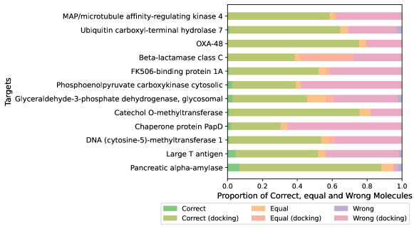
Figure S5: Bar plot of the proportion of correct, equal and wrong generated molecules. Molecules evaluated by retrieval and molecules evaluated by docking are distinguished using different colors.

We observe that NatureLM can successfully improve the molecule’s binding affinity by making small modifications on its chemical components, much like what a chemist would typically do (Fig. 8b). Compared with GPT-4, NatureLM can generate more molecules (Fig. 8a) with higher binding affinity, making it a better tool for molecule optimization than general domain LLM. Another observation is that more than 90% molecules generated by NatureLM do not have known binding affinity score in ChEMBL database. For 8 out of the 12 targets, over 50% of the generated novel molecules successfully decreased the docking scores (Fig. S5), demonstrating the model’s potential in exploring chemical spaces and discovering new drugs. We observe that NatureLM (8x7B) and NatureLM (8B) outperform NatureLM (1B) as they generate more correct molecules for the majority of targets (Fig. S6).

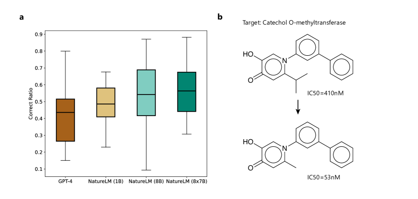
Figure 8: Evaluation of text-guided binding affinity optimization. (a) Box plot of the correct ratios of GPT-4, NatureLM (1B), NatureLM (8B) and NatureLM (8x7B) on 12 targets. (b) A case on the binding affinity optimization for Catechol O-methyltransferase. With small modifications, the binding affinity improves from 410nM to 53nM.

3.6 Text-guided metabolism & distributional property optimization

We next assess the molecular optimization capabilities of NatureLM regarding metabolism and its potential to cross the blood-brain barrier (BBB), a crucial factor in drug distribution. For metabolism, the goal is to reduce the inhibition of five key metabolic enzymes: CYP1A2, CYP2C19, CYP2C9, CYP2D6 and CYP3A4. An example is shown below:

Example 3.4.

Instruction:
Transform $\langle$mol$\rangle$COCCn1c(=O)c(-c2ccccc2)nc2cnc(N3CCOCC3)nc21$\langle$/mol$\rangle$ to yield lower CYP1A2 inhibition and present a better metabolic safety record.
Response:
$\langle$mol$\rangle$COc1ccc(-c2nc3cnc(N4CCOCC4)nc3n(Cc3cccc(OC)c3)c2=O)cc1$\langle$/mol$\rangle$

In terms of BBB permeability (BBBP), we evaluate the enhancement BBB permeability. An example is provided below:

Example 3.5.

Instruction:
Adjust the molecule $\langle$mol$\rangle$CC[C@H](NC(=O)c1c(OCCCC(=O)O)c

(-c2ccccc2)nc2ccccc12)c1ccccc1$\langle$/mol$\rangle$ to facilitate its passage through the blood-brain barrier.
Response:
$\langle$mol$\rangle$CC[C@H](NC(=O)c1c(O)c(-c2ccccc2)nc2ccccc12)c1ccccc1$\langle$/mol$\rangle$

For each test sample, we used random search to generate four cases. To determine whether NatureLM effectively refined the input molecule, we trained six groups of deep learning models for this evaluation. For assessing BBBP, we utilized the state-of-the-art model, BioT5 PeiQizhi2023BioT5 , to determine whether a compound is capable of crossing the BBB. For metabolism optimization, we used ChemProp yang2019analyzing to train classifiers to test if a molecule has the ability to inhibit enzymes from the cytochrome P450 (CYP) superfamily. We evaluated the percentage of molecules that were successfully optimized according to the specified criteria (see Section C.3 for details).

Table 6 displays the outcomes of BBBP and metabolism optimization. The success rates for optimizing BBBP with the 1B, 8B, and 8x7B versions of NatureLM are 0.482, 0.549, and 0.552, respectively. Larger models show better performance, though the improvement is not substantial. This suggests potential for enhancement opportunities in the future. For metabolism optimization, generally, the 8B model outperforms the others in terms of success rate, followed by the 8x7B model and lastly the 1B model. The 1B and 8B models share the same architecture (dense models, large vocabulary size), whereas the 8x7B model has a distinct one (mixture-of-expert model, relative small vocabulary size). In this particular task, the progression from the 1B model to the 8B model is consistent. However, a detailed analysis contrasting the 8x7B model is to be conducted in subsequent studies. Additionally, we jointly optimized metabolism and a basic property. The findings indicate that larger models generally yield better results (see Table S5).

	BBBP	CYP1A2	CYP2C19	CYP2C9	CYP2D6	CYP3A4	CYP Average
1B	0.482	0.805	0.815	0.770	0.750	0.831	0.794
8B	0.549	0.882	0.813	0.882	0.833	0.913	0.865
8x7B	0.552	0.837	0.834	0.838	0.812	0.853	0.835

Table 6: Optimization results of BBBP metabolism and CYP enzymes. Measured by success rate.

3.7 Retrosynthesis prediction

Retrosynthesis aims to identify synthesis routes for target molecules using commercially available compounds as starting points, a critical task in the discovery and manufacture of functional small molecules corey1969computer ; segler2018planning ; maziarz2024chimera . The applicability of ML-based retrosynthesis tools largely depends on the accuracy of single-step retrosynthesis prediction. We evaluate the capability of NatureLM for single-step retrosynthesis prediction on USPTO-50K  schneider2016uspto50k . NatureLM is prompted with the task description and the chemical SMILES of the product molecule, and is expected to generate potential reactants.

We followed the common practice for splitting the USPTO-50K dataset dai2019retrosynthesis ; maziarz2024re , and evaluated the performance using the 5007 reactions included in the test set. We ensured that there is no test set leakage in this setting. As outlined in Table 7, all sizes of NatureLM models surpass other methods in terms of top-$k$ accuracy, demonstrating our model’s accurate predictive ability for retrosynthesis prediction. NatureLM significantly outperforms GPT-4, a general LLM trained on human languages. This suggests that training on scientific data is crucial for models to excel in scientific tasks. Furthermore, NatureLM outperforms the state-of-the-art domain-specific models such as LocalRetro chen2021localretro and R-SMILES Zhong2022rsmiles , showing NatureLM’s potential as a scientific generalist in critical scientific tasks. We also note an increase in performance from NatureLM (1B) to NatureLM (8x7B), demonstrating the scaling advantages of larger models.

Example 3.6.

Instruction:
Please suggest possible reactants for the given product $\langle$product$\rangle$CC(=O)c1ccc2c(ccn2C(=O)OC(C)(C)C)c1$\langle$/product$\rangle$
Response:
$\langle$reactant$\rangle$ CC(=O)c1ccc2[nH]ccc2c1.CC(C)(C)OC(=O)OC(=O)OC(C)(C)C $\langle$/reactant$\rangle$

	Top-1 accuracy	Top-3 accuracy
GPT-4	22.4%	N/A
LocalRetro chen2021localretro	51.5%	76.5%
R-SMILES Zhong2022rsmiles	56.0%	79.1%
EditRetro han2024editretro	60.8%	80.6%
NatureLM (1B)	68.6%	86.8%
NatureLM (8B)	70.2%	85.9%
NatureLM (8x7B)	71.9%	87.4%

Table 7: Retrosynthesis prediction results on USPTO-50K dataset.

4 Protein tasks

Our model’s capabilities with respect to proteins are assessed through several distinct types of tasks:

1. Unconditioned protein generation: The model generates protein sequences from scratch without any specific conditions or prompts.

2. Text-guided protein generation: This task involves guiding the model to generate protein sequences based on given natural language descriptions.

3. Antibody design: The model designs the Complementary-Determining Region H3 (CDR-H3) of antibodies to effectively bind to target antigens.

4. Protein description generation: This task focuses on generating explanations or uncovering properties and functions of protein sequences, articulating them in natural language.

4.1 Unconditioned generation

The first capability of the model is generating protein sequences from scratch freely, prompted by the start token for proteins only, i.e., $\langle$protein$\rangle$. However, since there is no golden standard for evaluating proteins when no conditions are specified, it is difficult to measure the generation results. We focus on foldability, measured by pLDDT score Mariani2013-av , as well as lengths and diversity of the sequences, for the valid sequences.

Model	Avg Length	Diversity	AVG pLDDT
Mixtral 8x7b	53.3	0.906	69.9
GPT-4	45.7	0.816	65.1
NatureLM (1B)	288.3	0.985	69.8
NatureLM (8B)	284.5	0.973	71.8
NatureLM (8x7B)	318.4	0.989	75.9

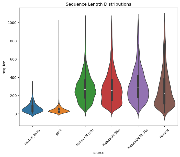
Figure S11: Sequence length distribution of generated proteins. The NatureLM models demonstrate a more natural distribution that closely resembles the reference UR50 sequences, while Mixtral 8x7B and GPT-4 tend to generate shorter sequences.

Table 8: Protein Sequence Generation Comparison. The average length of natural proteins (calculated from a subset of proteins randomly sampled from UR50) is about 311. The diversity was calculated by the number of clusters with 50% sequence identity divided by the total generated sequence count. The pLDDT scores were calculated by OmegaFold omegafold on the generated sequences with length less than 100 for a fair comparison. The length distribution is left in Figure S11.

As shown in Table 8, NatureLM consistently outperform Mixtral 8x7b and GPT-4 in terms of average sequence length, diversity, and average pLDDT score. The NatureLM (8x7B) model achieves the best performance across all metrics, with an average length of 318.4, diversity of 0.989, and average pLDDT score of 75.9. ProLLAMA lv2024prollamaproteinlanguagemodel a fine-tuned LLM for protein. It generates proteins without explicitly defined constraints on length, achieving a pLDDT score of 66.5. In contrast, our approach, which does not impose length constraints, results in pLDDT scores of 69.8 and 78.1 for the 8B and 8x7B models, respectively, demonstrating our significant advancement in this area.

4.2 Text-guided protein generation

For text-guided protein generation, we evaluated our models’ ability to generate proteins with specific properties based on natural language prompts. In this study, we focused on two key properties: solubility and stability, leaving the exploration of additional properties for future work. For stability, the models were tasked with generating protein sequences that exhibit stable properties. Regarding solubility, since both soluble and insoluble proteins are common in natural sequences, we instructed NatureLM to generate sequences of both types. Sample prompts are shown below, and a full list of prompts can be found in Figure S13.

Example 4.1.

$\rhd$ An example prompt for “stable protein generation”
I require a stable protein sequence, kindly generate one.
$\rhd$ An example prompt for “soluble protein generation”
Generate a soluble protein sequence.
$\rhd$ An example prompt for “insoluble protein generation”
Produce a protein sequence that is not soluble.

To evaluate the stability and solubility of a generated protein sequence, we utilized two specialist models fine-tuned from the protein foundation model, SFM-Protein he2024sfm , as oracle models. One model was used for stability classification, while the other was used for solubility classification. The oracle models provide probabilities that suggest the likelihood of the sequence possessing the desired property. To verify the efficiency of our model against random sampling, we have also chosen a subset of 1000 natural protein sequences from the UR50 dataset and assessed them using the same oracle models.

Source	AVG Prediction	Data Ratio (Score $>0.5$)
Natural	0.552	0.704
NatureLM (1B)	0.559	0.644
NatureLM (8B)	0.619	0.757
NatureLM (8x7B)	0.655	0.812

Table 9: Stability score ratio of the generated sequences.

Figures LABEL:fig:protein:conditioned_generation_stability and LABEL:fig:protein:conditioned_generation_solubility show the distributions of stability and solubility scores for the generated sequences, respectively. The NatureLM models demonstrate controlled distribution shift in generating proteins with desired properties compared to the natural sequences. In the task of generating more stable proteins, as shown in Figure LABEL:fig:protein:conditioned_generation_stability, a clear trend emerges: as the model size increases, the proportion of sequences classified as stable grows, with a pronounced peak in the NatureLM (8x7B) results. The quantified data, summarized in Table 9, further supports this observation. All three models produce proteins that are more stable than natural sequences based on average stability scores. Additionally, two of the models outperform natural proteins in terms of the number of sequences that exceed a stability threshold of 0.5. For the solubility condition, Figure LABEL:fig:protein:conditioned_generation_solubility reveals a similar trend. As the model size increases, the separation between the distributions of soluble and insoluble scores becomes more distinct, with less overlap.

4.3 Antigen-binding CDR-H3 design

The task of antigen-binding CDR-H3 design focuses on constructing the Complementary-Determining Region H3 (CDR-H3) of an antibody to bind effectively to a target antigen. We employed the RAbD benchmark dataset adolf2018rabd , comprising 60 antibody-antigen complexes. The example is shown below:

Instruction:
Using antigen $\langle$protein$\rangle$TQVCTGTDMKLR$\cdots$GESSEDCQS$\langle$/protein$\rangle$ and antibody frameworks $\langle$antibody$\rangle$IVLTQTPS$\cdots$LAVYYC$\langle$/antibody$\rangle$ and $\langle$antibody$\rangle$FGGGTRLEIEVQ$\langle$/antibody$\rangle$, create the CDR3 regions.
Response:
$\langle$antibody$\rangle$QQYSNYPWT$\langle$/antibody$\rangle$

The generation quality is evaluated by the Amino Acid Recovery (AAR) scores for the CDR-H3 design task. We use $r$ and $\hat{r}$ to represent the reference and generated sequences respectively, while $L(r)$ and $L(\hat{r})$ denote the number of amino acids in $r$ and $\hat{r}$. The $i$-th residue in the two sequences is denoted by $r_{i}$ and $\hat{r}_{i}$. The AAR is defined as follows:

$${\rm AAR}(r,\hat{r})=\frac{1}{L(r)}\sum_{i=1}^{L(r)}\mathbb{I}(r_{i}=\hat{r}_{i}).$$ (1)

In case $L(\hat{r})>L(r)$, only the first $L(r)$ elements are verified. If $L(\hat{r})<L(r)$, we assign $\mathbb{I}(r_{i}=\hat{r}_{i})=0$ for $i>L(\hat{r})$.

Method	AAR ($\uparrow$)
GPT-4	0.312
RefineGNN jin2021refinegnn	0.298
HSRN jin2022hsrn	0.327
MEAN kong2022mean	0.368
ABGNN gao2023abgnn	0.396
Llama 3 (8B)	0.275
NatureLM (1B)	0.273
NatureLM (8B)	0.368
NatureLM (8x7B)	0.376

Table 10: AAR of the CDR-H3 design. Please note that the NatureLM models utilize sequence-only input for this task, whereas the baseline models may incorporate additional information, such as structural data.

Table 10 presents the Amino Acid Recovery (AAR) scores for the CDR-H3 design task. As the model size of NatureLM increase, the AAR gradually increases. The NatureLM (8x7B) model achieves competitive performance with an AAR of 0.376, outperforming several specialized GNN-based models. While SFM-protein, a BERT-like model trained on protein sequences, holds the top performance, our results demonstrate the potential of NatureLM in CDR-H3 design, particularly as the model scales and undergoes further refinement.

4.4 Protein description generation

Despite the rapid discovery of natural protein sequences facilitated by advanced sequencing techniques, the functions of many of these proteins remain largely unknown. This knowledge gap restricts our ability to exploit these proteins for engineering and therapeutic purposes. In this study, we explored the annotation generation capabilities of the NatureLM series.

To achieve this, we compiled pairs of protein sequences and their human-readable annotations from various species, sourced from the NCBI database. We divided the dataset temporally: historical data were utilized for training the NatureLM models, while annotation data from the most recent four months were reserved for testing. Model performance was evaluated using Rouge-L scores. As shown in Table 11, NatureLM models consistently outperformed Llama 3 8B in Rouge-L scores, with performance differences widening as model size increased. Notably, the NatureLM (8x7B) model achieved the highest score of 0.585. A detailed analysis presented in Figure 14 revealed that the NatureLM (8x7B) model not only generates protein annotations with greater accuracy but also successfully identifies orthologues and functions of proteins, while NatureLM (8B) is also able to generate reasonable results in many cases.

Model Setting	Rouge-L
Fine-tuned Llama 3 (8B)	0.324
NatureLM (1B)	0.548
NatureLM (8B)	0.572
NatureLM (8x7B)	0.585

Table 11: Performance of protein description generation, measured by Rouge-L. Llama 3 (8B) serves as a baseline, which is directly fine-tuned on the data collection described in Section 2.2. More details about this baseline in Section 10.

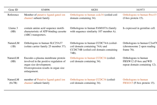
Figure 14: Generated descriptions for different proteins.

In conclusion, NatureLM demonstrates strong performance across a wide range of protein-related tasks, from unconditioned generation to specific design tasks like CDR-H3 design. The scalability of our approach is evident, with larger models consistently outperforming smaller versions and often achieving state-of-the-art results.

5 Material tasks

To evaluate the capabilities of NatureLM for material generation, it is prompted to generate material’s compositions in both unconditional and conditional way. For unconditional generation, the model is prompted with a special token indicating the start of material (i.e., $\langle$material$\rangle$) and is expected to generate the composition of the material (Section 5.1). For conditional generation, the model is prompted to generate material formula and structure under specific human instructions, including: (1) Composition to material generation (Section 5.2); (2) Bulk modulus to material generation (Section 5.3). After generating the chemical formula of a material, we use a dedicated fine-tuned NatureLM to generate its crystal structures, which are then evaluated for their accuracy and stability (see Section 5.4).

5.1 Unconditional material generation

The model is tasked with generating materials with arbitrary compositions. The input to NatureLM is $\langle$material$\rangle$, and it produces material compositions with a specified space group. An example is provided below,

Example 5.1.

Instruction: $\langle$material$\rangle$
Response: $\langle$material$\rangle$ A A B B B $\langle$sg12$\rangle$$\langle$/material$\rangle$

where A, B refer to elements and $\langle$sg12$\rangle$ denotes the space group.

We evaluated the SMACT validity of the generated materials. Furthermore, we used the dedicated fine-tuned NatureLM to autoregressively predict the crystal structures of a randomly chosen subset of valid compositions (see Section 5.4). The energy above hull (abbreviated as ehull) of the predicted structures was then evaluated using MatterSim yang2024mattersim . The distribution of ehull is shown in Fig. LABEL:fig:mat_uncon. We also assessed the ratio of stable materials, defining a generated material as stable if its ehull$<0.1$eV/atom. The results are presented in Table 12. It is evident that as the model size increases, the SMACT validity and stability of the generated materials improve.

Model	SMACT (%)	Stability (%)
NatureLM (1B)	49.20	10.12
NatureLM (8B)	63.42	12.47
NatureLM (8x7B)	66.07	17.86

Table 12: The SMACT validity and stability (with ehull$<0.1$eV/atom) for unconditional material generation. The distribution of ehull for the generated materials is illustrated in Fig. LABEL:fig:mat_uncon.

5.2 Composition to material generation

The model is tasked with generating materials containing specific elements:

Example 5.2.

Instruction: Build a material that has Li, Ti, Mn, Fe, O
Response: $\langle$material$\rangle$ Li Li Li Li Ti Ti Ti Mn Mn Fe Fe Fe O O O O O O O O O O O O O O O O $\langle$sg8$\rangle$$\langle$/material$\rangle$

We evaluated the SMACT validity, stability, novelty, and precision of the generated materials. The novelty is measured as the ratio of unique generated materials that are not present in our instruction tuning data. The composition precision is calculated as

$${\rm composition\ precision}=\frac{1}{N}\sum_{i=1}^{N}\frac{\lvert E_{pi}\cap E_{gi}\rvert}{\lvert E_{pi}\rvert},$$ (2)

where $E_{pi}$ and $E_{gi}$ stand for the sets of elements in the $i$-th prompt and corresponding generated material respectively.

The results are demonstrated in Table 13, and the distribution of ehull is depicted in Figure LABEL:fig:mat_comp_to_mat_ehull. Table 13 shows a significant improvement in SMACT validity scores due to instruction tuning compared to unconditional generation. The precision for all three models is close to 100%, indicating their strong capability to follow language instructions for generating material formulas with expected elements. Additionally, the high novelty demonstrates the models’ generative abilities. Furthermore, stability improves with model size, highlighting their scalability. Figure LABEL:fig:mat_comp_to_mat_ehull illustrates this more clearly: as model size increases, the ehull distribution shifts closer to zero, indicating that more materials have lower energy and are in a more stable state.

Model	SMACT (%)	Stability (%)	Precision (%)	Novelty (%)
NatureLM (1B)	79.38	31.56	97.95	97.13
NatureLM (8B)	83.36	35.56	98.44	95.51
NatureLM (8x7B)	81.56	36.46	97.68	94.83

Table 13: The SMACT validity, stability, precision, and novelty for composition to material generation.

5.3 Bulk modulus to material generation

The bulk modulus of a substance is a measure of the resistance of a substance to bulk compression. As a proof-of-concept, the model is prompted to generate materials with specified bulk modulus:

Example 5.3.

Instruction: Construct the composition for a material with a specified bulk modulus of 86.39 GPa.
Response: $\langle$material$\rangle$ Se Se Pd Sc $\langle$sg164$\rangle$$\langle$/material$\rangle$

We evaluated the SMACT validity, stability, novelty, and precision of the generated materials. Precision is defined as the ratio of generated materials whose bulk modulus is within 10% of the instructed value, compared to all generated materials.

The results in Table 14 indicate improved SMACT validity and stability as the model scales. Figure LABEL:fig:mat_bulk_to_mat_ehull depicts the distribution of ehull for the generated materials, showing a shift closer to zero with increasing model size.

Further, to demonstrate how NatureLM follows the instruction to generate materials with expected bulk modulus, we depict the distribution of the bulk modulus of generated materials under the instructions in Figure 18 where the $x$-axis denotes the bulk modulus in the instruction prompt and the $y$-axis denotes the bulk modulus of the generated materials under the corresponding instruction. We can see that, as the model scales, the distribution aligns more closely with the ideal linear diagonal.

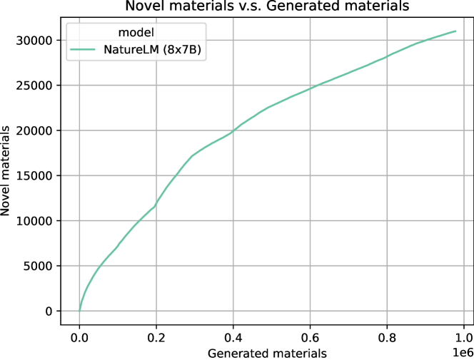
Figure S10: Novel materials w.r.t generated materials.

To assess how many novel materials NatureLM can generate, we prompted the model with a single instruction and allowed it to produce up to 1,000,000 material formulas. We then plotted the count of novel material formulas against the total number generated. Novel materials are defined as those passing the SMACT validity check, not present in the instruction tuning data, and not previously generated. Figure S10 shows that the number of novel materials increases with the total generated. Even at 1 million generated materials, novel ones continue to appear, highlighting the model’s strong generative capability.

Model	SMACT (%)	Stability (%)	Precision (%)	Novelty (%)
NatureLM (1B)	86.76	39.34	40.00	52.38
NatureLM (8B)	87.21	52.81	44.06	36.31
NatureLM (8x7B)	94.75	53.60	44.62	32.42

Table 14: The SMACT validity, stability, precision, and novelty of generated materials conditioned on bulk modulus.

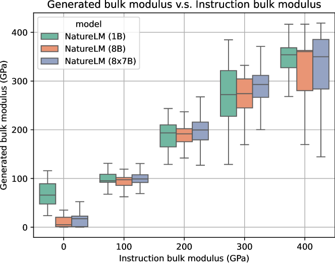
Figure 18: Distributions of bulk modulus of generated materials.

5.4 Crystal structure prediction for materials

Crystal material structure prediction (CSP) is a critical problem. Previous works apply random search, particle swarm algorithm, and a few others search algorithms to look for stable crystal structures. More recently, generative models like VAE cdvae , diffusion zeni2023mattergen and flow matching based methods flowmm are applied for such 3D structure generation. There is also a growing trend towards using Large Language Models (LLMs) for crystal structure generation, which can autoregressively generate the structures gruver2024finetunedlanguagemodelsgenerate ; antunes2024crystalstructuregenerationautoregressive ; flowmm . We fine-tune NatureLM to act as a crystal structure prediction module that generates 3D structures in an autoregressive manner.

Using NatureLM for structure prediction is particularly meaningful because it aligns the sequential modeling capacity of LLMs with the sequential representation of crystal structures. This congruence allows the model to capture the intricate dependencies and patterns inherent in material structures, potentially leading to more accurate and efficient generation of stable crystal configurations.

We represent materials and their 3D structures as 1D sequences in three steps:

1. Flatten the chemical formula: Repeat each element according to its count (e.g., A2B3 becomes A A B B B).

2. Add space group information: Append special tokens $\langle$sg$\rangle$ and $\langle$sgN$\rangle$, where N is the space group number.

3. Include coordinate information: Use the token $\langle$coord$\rangle$ to indicate the start of coordinates. Flatten the lattice parameters into nine float numbers and the fractional atomic coordinates into sequences of float numbers. Numbers are retained to four decimal places and tokenized character-wise (e.g., -3.1416 as - 3 . 1 4 1 6).

For example, the sequence for a material A2B3 with space group number 123 is:

Example 5.4.

A A B B B $\langle$sg$\rangle$ $\langle$sg123$\rangle$ $\langle$coord$\rangle$ 9 float numbers for lattice 15 float numbers for atoms

We collect data from Materials Project materialsproject , NOMAD nomad and OQMD oqmd2013 ; oqmd2015 as our training data which are widely used database for materials with structure information, and test on MP-20, Perov-5 and MPTS-52 following previous works cdvae ; diffcsp ; flowmm . Specially, we remove duplications in the merged training data and remove all the data that appear in the test set in these benchmarks. The final training data contains about 6.5M samples after deduplication and removal of the test set. After training, we also finetuned the model on the training set for each benchmark to mitigate the different distributions between our training data and the benchmark data. We evaluate the match rate of the generated material structures and compare to CDVAE cdvae , DiffCSP diffcsp and FlowMM flowmm . The results are shown in Table 15. Experiment results show that our sequence based auto-regressive method achieves comparable or best performance on MP-20 and MPTS-52 compared to other methods. We will use this for material structure generation in our following experiments. In future work, we will leverage and combine with more advanced methods like MatterGen zeni2023mattergen for structure generation.

	Perov-5		MP-20		MPTS-52
	MR (%)	RMSE	MR (%)	RMSE	MR (%)	RMSE
CDVAE	45.31	0.1138	33.90	0.1045	5.34	0.2106
DiffCSP	52.02	0.0760	51.49	0.0631	12.19	0.1786
FlowMM	53.15	0.0992	61.39	0.0566	17.54	0.1726
NatureLM (1B)	50.78	0.0856	61.78	0.0436	30.20	0.0837

Table 15: The match rate (MR) and RMSE on Perov-5, MP-20 and MPTS-52.

The fine-tuned NatureLM (1B) achieves performance that is comparable to or surpasses other state-of-the-art methods. The high match rates and low RMSE values demonstrate that our model effectively captures the complex spatial arrangements of atoms in crystal structures. Moreover we can see that NatureLM performs better than other methods as the number of atoms increases, demonstrating the advantage of autoregressive sequence model. As a next step, we plan to further improve the structure prediction quality by incorporating 3D autoregressive data into the pre-training phase of the next version of NatureLM.

6 Nucleotide tasks

The genome contains a vast amount of information regarding protein-coding genes and the regulatory DNA and RNA sequences that control their expression. In this section, we evaluated our model on nucleotide sequence generation tasks, including both unconditional generation and cross-domain generation, specifically DNA to RNA generation (guide RNA design) and protein to RNA generation.

6.1 Unconditional RNA generation

Designing RNA molecules is crucial for advancing RNA vaccines, nucleic acid therapies, and various biotechnological applications. In this section, we evaluate the proficiency of NatureLM in generating RNA sequences without any conditional prompts. For evaluation purposes, we constrained the generated RNA sequences to a maximum length of 1024 nucleotides. An example of an unconditionally generated sequence is provided below:

Example 6.1.

Instruction: $\langle$rna$\rangle$
Response: $\langle$rna$\rangle$ C C A C G G A G C C $\langle$/rna$\rangle$

We assessed the quality of the generated RNA sequences by calculating their Minimum Free Energy (MFE) using RNAfold Lorenz2011 (see Section C.2 for details). A lower MFE value indicates a potentially more stable RNA secondary structure. For each model, we generated 5,000 sequences and computed their MFE values. To establish a baseline for comparison, we generated control sequences and computed their average MFE values. Specifically, for each generated sequence, we created:

(1) Shuffled Sequences: For each generated sequence, we created a new sequence by randomly shuffling its nucleotides, thereby preserving the original nucleotide composition and length but potentially disrupting any inherent structural motifs.

(2) Random Sequences: For each generated sequence, we created an entirely random sequence of the same length, where each nucleotide position was independently sampled from the four nucleotides (A, G, C, U) with equal probability. This baseline represents sequences with no designed structure or composition bias.

As a reference for the MFE values of natural RNA sequences, we randomly sampled 5,000 sequences of length up to 1,024 nucleotides from RNAcentral and computed their MFE values.

The average MFE values are reported in Table 16.

	MFE (kcal/mol)	Retrieved Rfam Families
RNAcentral	-165.4
Shuffled sequences	-156.4
Random sequences	-142.0
NatureLM (1B)	-160.6	23
NatureLM (8B)	-170.6	38
NatureLM (8x7B)	-177.1	165

Table 16: Average MFE values (in kcal/mol) of RNA sequences generated by different methods and the number of unique Rfam families retrieved by different models. MFE denotes the mean Minimum Free Energy of the sequences. Retrieved Rfam Families represents the count of unique RNA families identified in the generated sequences using cmscan.

From the results, we observe that larger models tend to generate RNA sequences with lower (more negative) MFE values, indicating potentially more stable secondary structures. Additionally, shuffling and randomizing the sequences result in higher (less negative) MFE values, suggesting that the original sequences generated by our models have structural features that contribute to stability.

To evaluate the diversity of the RNA sequences generated by NatureLM, we compared them to known RNA families in Rfam 10.1093/nar/gkaa1047 . We used cmscan from the Infernal toolkit 10.1093/bioinformatics/btt509 to search for structural similarities between our generated sequences and the Rfam database (see Section C.2 for details). As shown in Table 16, larger models retrieved a significantly higher number of unique Rfam families than smaller models: the 1B, 8B, and 8x7B models retrieved 23, 38, and 165 unique families, respectively, covering a wider range of RNA functions. These results suggest that larger models not only generate more stable sequences but also encompass a more diverse set of RNA structures and functions.

6.2 Guide RNA design

Guided RNA, commonly referred to as guide RNA (gRNA), is a key element in CRISPR-Cas9 gene-editing technology. It is essential for directing the Cas9 enzyme to a precise location within the genome where genetic modifications are intended. We evaluate NatureLM on two gRNA design tasks: the first is designing gRNAs for a given DNA sequence, and the second is selecting the more effective gRNA from two candidates. Examples are provided below:

Example 6.2.

$\rhd$gRNA generation
Instruction:
Generate a guide RNA for targeting the DNA sequence
$\langle$dna$\rangle$GACTGGCACCAG$\cdots$CCCTCGC$\langle$/dna$\rangle$.
Response: $\langle$rna$\rangle$AGACACAGCGGGTGCTCTGC$\langle$/rna$\rangle$

$\rhd$More effective gRNA identification
Instruction: Investigate which of $\langle$rna$\rangle$ATGTAGAAGAATCCACC
ATA$\langle$/rna$\rangle$ or $\langle$rna$\rangle$GGAAGGGGTCAATATTCTCA$\langle$/rna$\rangle$ results in better wild-type efficiency for the DNA sequence
$\langle$dna$\rangle$AAGGGGTGGCA$\cdots$AGTGC$\langle$/dna$\rangle$.

Response: $\langle$rna$\rangle$ATGTAGAAGAATCCACCATA$\langle$/rna$\rangle$

A valid gRNA is defined by the following criteria: (1) the length of the generated gRNA must be between 17 to 24 nucleotides; (2) the generated sequences should match a region in the given DNA sequences; (3) the matched sequence in the DNA template must be directly followed by an “NGG” sequence, known as the Protospacer Adjacent Motif (PAM).

NatureLM demonstrates a strong ability to generate valid gRNA sequences compared with generalist models like GPT4, accurately targeting the specified DNA while maintaining the PAM sequence feature. Furthermore, NatureLM shows proficiency in assessing the effectiveness of gRNAs, enabling it to select the more efficient gRNA from a given pair (Table 17).

Model	Validity	Top 1 accuracy
GPT-4	0.272	0.597
Llama 3 8B	0	0.38
Mixtral 8x7B	0	0.46
NatureLM (1B)	0.95	0.681
NatureLM (8B)	0.765	0.657
NatureLM (8x7B)	0.957	0.699

Table 17: The performance of guide RNA design.

6.3 Protein binding RNA design

RNA-binding proteins (RBPs) represent a large and diverse class of over 2,000 proteins that play a crucial role in regulating gene expression by interacting with RNA. Designing RNA decoys offers a powerful strategy to manipulate these interactions. Such decoys can sequester RBPs away from their natural RNA targets, act as competitors to displace natural RNA molecules from RBPs, or serve as scaffolds to recruit RBPs to specific RNA molecules or cellular locations.

Example 6.3.

Instructions: Given $\langle$protein$\rangle$MSEY$\cdots$SSGWGM$\langle$/protein$\rangle$, create an RNA molecule that binds to it.
Response: $\langle$rna$\rangle$AAACAGG$\cdots$CGTACGACA$\langle$/rna$\rangle$

We selected 200 targets and generated binding RNA for them. To evaluate the generation ability of NatureLM, following xu2023prismnet , we trained a predictor for each protein to predict the binding affinity between the RNA and the protein. Specifically, the final layer of the classifier is a sigmoid function, which produces an output value ranging from 0 to 1, indicating the strength of the RNA-protein binding. If the score is greater than 0.5, we consider the generated RNA to have successfully bound to the protein.

We compared the RNA sequences generated by NatureLM 1B, 8B and 8x7B. Additionally, we used the predictors to evaluate the binding and non-binding RNA sequences from the test set. We also randomly selected RNA sequences of the same sizes from the unconditional generation setting for prediction (Section 6.1).

The results are summarized in Table 18, which reports the average and median prediction scores, as well as the success rate—the proportion of sequences with a prediction score above 0.5. We have the following observations:

1. As expected, binding RNA sequences achieved the highest average prediction score of 0.714 and a success rate of 74.5%, while the non-binding RNA sequences had the lowest average score of 0.274 and a success rate of 24.4%. This confirms the reliability of the classifiers and serving as a benchmark for optimal performance.

2. For unconditioned RNA Sequences, with an average score of 0.391 and a success rate of 36.3%, these sequences performed better than non-binding sequences but significantly worse than the binding sequences. This suggests that random RNA sequences have a moderate chance of being predicted as binders due to the intrinsic properties of RNA but lack the specificity achieved through conditioning.

3. For NatureLM generated sequences, as we increase the model sizes, there is a clear trend that larger models perform better. The results also demonstrated that NatureLM is more likely to generate RNA sequences that are likely to bind to the specified proteins when explicitly conditioned on them.

Source	AVG Score	Success rate (%)
Binding	0.714	74.5
Non-binding	0.274	24.4
Unconditioned	0.391	36.3
NatureLM (1B)	0.415	40.9
NatureLM (8B)	0.434	44.2
NatureLM (8x7B)	0.438	44.8

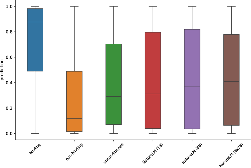
Figure S12: The distribution of the predicted scores for the RNA sequences in the test set and the generated RNA sequences shows a clear trend. In terms of median values, larger models consistently achieve better predicted scores, indicating stronger binding affinity.

Table 18: Performance of designing protein-binding RNA given proteins: “AVG Scores” refers to the average prediction scores across all sequences. Success ratio refers to the percentage of scores that are greater than 0.5. See Figure S12 for the detailed distribution of the predicted scores.

.

7 Prediction tasks

In addition to the generation and design tasks studied in previous sections, we also studied the predictive capabilities of NatureLM.

7.1 Small molecule prediction tasks

We evaluated NatureLM on three molecular property prediction tasks from MoleculeNet moleculenetpaper : (i) predicting whether a molecule can cross the blood-brain barrier (BBBP); (ii) predicting whether a molecule can bind to the BACE receptor (BACE); (iii) predicting the toxicity of a molecule associated with 12 targets (Tox21). An illustrative example is presented below:

Example 7.1.

Instruction:
Can $\langle$mol$\rangle$C1(c2ccccc2)=CCN(C)CC1$\langle$/mol$\rangle$ traverse the blood-brain barrier?
Response:
Yes.

Instruction:
Could the compound $\langle$mol$\rangle$N(O)=C1CCC([NH2+]CC(O)C (Cc2cc(F)cc(F)c2)NC(C)=O)(c2cccc(C(C)(C)C)c2)CC1$\langle$/mol$\rangle$ potentially restrain beta-secretase 1?
Response:
Yes.

To determine the probability of a “Yes” or “No” response, we first extract the probabilities output by the NatureLM, denoting the probability of “Yes” as $p_{1}$ and the probability of “No” as $p_{2}$. We then normalized these probabilities: the probability of “Yes” is calculated as $p_{1}/(p_{1}+p_{2})$ while the probability of “No” is $p_{2}/(p_{1}+p_{2})$.

All tasks in this subsection are measured by AUROC. The results are reported in Table 19. Generally, larger models achieve better performance, while there is still a gap between the current NatureLM and the state-of-the-art specialist models.

	BBBP	Bace	Tox21
DVMP 2021jinhuaDVMP	78.1	89.3	78.8
BioT5 PeiQizhi2023BioT5	77.7	89.4	77.9
NatureLM (1B)	71.1	79.4	68.3
NatureLM (8B)	70.2	82.0	69.8
NatureLM (8x7B)	73.7	83.1	72.0

Table 19: Molecular property prediction on MoleculeNet moleculenetpaper . The evaluation metric is the AUROC score.

7.2 Protein prediction tasks

We evaluated the NatureLM on four protein property classification tasks, including solubility prediction, stability prediction, and protein-protein interaction (PPI) prediction for both human and yeast proteins. These datasets as well as the data splits are adopted from the PEER benchmark xu2022peer . An example is provided below:

Example 7.2.

Instruction:
Does the sequence of this protein suggest it would be stable? Please answer ‘Yes’ if it is stable and ‘No’ if it is not. $\langle$protein$\rangle$TTIKVNG …KVTR$\langle$/protein$\rangle$
Response:
No.

Instruction: Could these proteins interact, considering their sequences? The first protein is
$\langle$protein$\rangle$MPPS …VETVV$\langle$/protein$\rangle$, the second protein is $\langle$protein$\rangle$MSLHF …PLGCCR$\langle$/protein$\rangle$. Please respond with ‘Yes’ if the proteins can interact and ‘No’ if they cannot.
Response:
Yes

Model Setting	Solubility	Stability	Human PPI	Yeast PPI
Literature SOTA	0.702	-	0.881	0.661
SFM-Protein (650M) he2024sfm	0.744	0.583	0.852	0.628
NatureLM (1B)	0.684	0.682	0.781	0.561
NatureLM (8B)	0.714	0.635	0.848	0.604
NatureLM (8x7B)	0.698	0.723	0.776	0.586

Table 20: Protein understanding task comparison (accuracy). Please note that the NatureLM models are trained for various diverse tasks in a unified way and evaluated separately on these tasks by the same model, while the state-of-the-art models are trained and tested individually for each task.

Table 20 presents the accuracy of our models on various protein understanding tasks. Overall, the results highlight that our unified NatureLM models perform competitively with task-specific models, even surpassing them in certain tasks like stability prediction. This demonstrates the effectiveness of our training strategy, where a single model can learn and generalize across diverse protein understanding tasks without the need for separate models for each task.

7.3 DNA prediction tasks

We selected two classification tasks to assess the model’s capability of identifying significant sequence motifs implicated in human gene regulation. These tasks include the identification of promoters and transcription factor binding sites. We utilized datasets from the Genome Understanding Evaluation (GUE, see Appendix B.2 of zhou2024dnabert2 for a summary), converting them into a format suitable for instruction tuning. An example is shown below:

Example 7.3.

Instruction:
Verify if there is a promoter region within $\langle$dna$\rangle$TGGACT$\cdots$TGAGCTC$\langle$/dna$\rangle$?
Response:
Yes.

Instruction:
Can the sequence $\langle$dna$\rangle$GCCTGCCAG$\cdots$AAAAC$\langle$/dna$\rangle$ be classified as a transcription factor binding site?
Response:
No.

Model	Promoter detection	Core promoter detection	TF binding
NT-2500M-multi dalla2023nucleotide	0.881	0.716	0.633
DNABERT2 zhou2023dnabert	0.842	0.705	0.701
NatureLM (1B)	0.805	0.571	0.524
NatureLM (8B)	0.827	0.595	0.549
NatureLM (8x7B)	0.835	0.602	0.560

Table 21: Performance comparison of various models on DNA property prediction tasks, evaluated using Matthews Correlation Coefficient (MCC).

Table 21 presents the results of our experiments, evaluated using the Matthews Correlation Coefficient (MCC). For the Transcription Factor Binding prediction task, we conducted separate predictions on specific ChIP-seq datasets: POLR2A ChIP-seq on human HUVEC, POLR2A ChIP-seq on human ProgFib, PAX5 ChIP-seq protocol v041610.1 on human GM12892, TRIM28 ChIP-seq on human U2OS, and MXI1 ChIP-seq on human H1-hESC produced by the Snyder lab. We then calculated the average performance across these datasets. Despite a performance gap between our models and the state-of-the-art, the observed improvements with increasing model sizes suggest potential for further advancements. These findings indicate that larger models may more effectively capture the complex regulatory motifs involved in human gene regulation.

8 Strategies to further improve performance

In this section, we examine two strategies to improve the model’s performance: reinforcement learning for scenarios with limited labeled data for fine-tuning specific tasks, and dedicated fine-tuning for cases where sufficient labeled data is available for particular tasks.

8.1 Reinforcement enhanced NatureLM

Reinforcement Learning with Human Feedback (RLHF) is well-established approach to enhance foundation models. This section explores how to utilize preference signals in RLHF, moving beyond reliance on direct supervised signals. For many generative tasks, where answers are open-ended and do not have a single correct solution, training with preference signals offers a more intuitive approach.

For RLHF training, we curated preference data from nine property optimization tasks related to small molecules: BBBP, BACE, LogP, Donor, QED, CYP1A2, CYP2C9, CYP2D6, and CYP3A4. Detailed descriptions of each task and the corresponding data quantities can be found in Table S6. In total, we compiled 179.5k data points. Note that we used all the data to enhance the post-trained NatureLM (8B), resulting in a single model for the nine tasks after RLHF.

The data is structured in a preference-based format, where each sample consists of a prompt, along with both an accepted and a rejected response. An example of this format is presented below:

Example 8.1.

Instruction:
Enhance the effectiveness of the molecule $\langle$mol$\rangle$COc1cc2c(c(OC)c1OC)-c1ccc(OC)c(=O)cc1[C@@H](NC(C)=O)CC2 $\langle$/mol$\rangle$ in penetrating the blood-brain barrier.
Accepted Response:
$\langle$mol$\rangle$COc1cc2c(c(OC)c1OC)-c1ccc(OC)c(=O)cc1C(NC(C)=O)CC2$\langle$/mol$\rangle$
Reject Response:
$\langle$mol$\rangle$COc1cc2c(c(OC)c1OC)-c1ccc(OC)c(=O)cc1[C@@H](NC(C)=O)
CC2$\langle$/mol$\rangle$

In the example above, the compound in the accepted response is capable of crossing the BBB, whereas the compounds in the instruction and rejected response cannot.

We leveraged Direct Preference Optimization (DPO) rafailov2024direct to enhance the molecule optimization ability of NatureLM. The loss of DPO algorithm is written as follows:

$$\mathcal{L}_{\text{DPO}}(\pi_{\theta}\semicolon\;\pi_{\text{ref}})=-\mathbb{E}_{(x,y_{w},y_{l})\sim\mathcal{D}}\left[\log\sigma\left(\beta\log\frac{\pi_{\theta}(y_{w}\mid x)}{\pi_{\text{ref}}(y_{w}\mid x)}-\beta\log\frac{\pi_{\theta}(y_{l}\mid x)}{\pi_{\text{ref}}(y_{l}\mid x)}\right)\right],$$ (3)

where $\pi_{\rm ref}$ is the model after post-training and fixed during DPO training, $\pi_{\theta}$ is the model to optimize and set to $\pi_{\rm ref}$ before DPO training, $x$ is the prompt, $y_{w}$ is the accepted response, $y_{l}$ is the reject response, and $\beta$ is a hyper-parameter.

Property	$\Delta$
QED	0.6
LogP	0.6
Donor	0.6
BBBP	2.9
BACE	3.5
CYP1A2	2.3
CYP2C9	0.7
CYP2D6	0.7
CYP3A4	1.0

Table 22: Results of the reinforcement optimization. Let $r_{1}$ and $r_{2}$ represent the outcomes before and after applying reinforcement, respectively, and let $\Delta$ denote the percentage improvement, i.e., $\Delta=(r_{2}-r_{1})/r_{1}\times 100\%$.

Table 22 shows the improvements of DPO training over the 9 property optimization tasks. Notably, the model had already undergone instruction tuning (the post-training in Section 3) prior to DPO training, and no new data was introduced during the DPO process. The results highlight how reformatting the data into a preference-based structure allows the DPO algorithm to improve performance across multiple tasks simultaneously.

Looking ahead, we plan to generate data on the fly in RLHF and utilize additional reward models to evaluate the properties of newly generated molecules, thereby creating better preference-based data.

8.2 Dedicated fine-tuning on retrosynthesis

We dedicatedly fine-tuned our NatureLM model to evaluate its performance against specialized models in the retrosynthesis prediction task, using a large-scale labeled dataset, the Pistachio reaction dataset mayfield2017pistachio , with 15 million reactions from U.S., European, and WIPO patents. To ensure data quality, we removed any invalid or duplicate reactions. The cleaned dataset was then randomly split into a training set with 3.1 million reactions and a test set with 34,000 reactions.

Before training, we preprocessed the input products and output reactants using a root-aligned SMILES format Zhong2022rsmiles . This format offers a clear one-to-one mapping between the product and reactant SMILES, thereby enhancing prediction efficiency. Additionally, we augmented the training dataset tenfold to further improve the model’s performance. As shown in Table 23, NatureLM (1B) demonstrates competitive performance, rivaling leading template-based models (e.g., LocalRetro) and template-free models (e.g., R-SMILES) on the large Pistachio dataset.

	Top-1 accuracy	Top-3 accuracy
LocalRetro chen2021localretro	40.8%	56.6%
R-SMILES Zhong2022rsmiles	51.2%	67.1%
NatureLM (1B)	51.4%	66.0%

Table 23: Retrosynthesis prediction results on Pistachio dataset.

8.3 Dedicated fine-tuning on Matbench

We fine-tuned our NatureLM 8B model on Matbench matbench , a benchmark for state-of-the-art machine learning algorithms that predict various properties of solid materials. Matbench is hosted and maintained by the Materials Project materialsproject . Following the approach in xie2023darwin , we fine-tuned a single model for three tasks from Matbench, rather than developing separate models for each task.

The results are presented in Table 26 to 26. Results of baseline models are collected from the official leader board. As can be seen, NatureLM achieves state-of-the-art performance on matbench_expt_gap and matbench_is_metal.

Model	MAE $\downarrow$
Dummymatbench	1.1435
gptchemJablonka_2023	0.4544
RF-SCM/	0.4461
Magpiematbench
AMMExpressmatbench	0.4161
MODNetDe_Breuck_2021	0.3327
Ax/SAASBO	0.3310
CrabNetWang2021crabnet ; erikssonHighDimensionalBayesianOptimization2021
DARWINxie2023darwin	0.2865
NatureLM	0.2858

Table 24: Results on matbench_expt_gap.

Model	F1 $\uparrow$
Dummymatbench	0.4913
gptchemJablonka_2023	0.8953
MODNetDe_Breuck_2021	0.9153
RF-SCM/	0.9159
Magpiematbench
AMMExpressmatbench	0.9200
DARWINxie2023darwin	0.9599
NatureLM	0.9630

Table 25: Results on matbench_is_metal.

Model	F1 $\uparrow$
Dummymatbench	0.7127
DARWINxie2023darwin	0.8722
gptchemJablonka_2023	0.8782
RF-SCM/	0.9278
Magpiematbench
AMMExpressmatbench	0.9043
MODNetDe_Breuck_2021	0.9784
NatureLM	0.8720

Table 26: Results on matbench_glass.

9 Text capabilities

We assess the text-related capabilities of NatureLM (8x7B) in this section. We first present several examples to provide readers with an intuitive understanding (Section 9.1), and then benchmark results from AlpacaEval (Section 9.2).

9.1 Case study

Here we demonstrate our model’s language capabilities in scientific discovery research. Specifically, we assessed the model’s understanding of CRISPR gene editing, cancer immunotherapy, and drug discovery. A few selected cases are presented in this section for brevity. Additional cases can be found in Fig. S14, S15 and S16.

9.1.1 CRISPR gene editing

CRISPR gene editing has rapidly emerged as a powerful tool in biotechnology. Our model demonstrates a good understanding of CRISPR and is able to effectively analyze the advantages and disadvantages of commonly used CRISPR tools.

Instruction: Could you provide me the advantages and disadvantages of Cas9?
Response:
Advantages: 1. Highly efficient and specific gene editing with a low risk of off-target effects. 2. Can target a wide range of sequences. 3. Cam be used to make specific alterations to genes in virtually any organism. Disadvantages: 1. Potential for off-target effects when using Cas9. 2. The delivery of Cas9 can be inefficient. 3. Lack of control over the repair mechanism. 4. May cause chromosomal abnormalities.
Instruction: Could you provide me the advantages and disadvantages of Cas12a, another widely used CRISPR protein?
Response:
Advantages:
1. High specificty: Cas12a has higher specificity compared to Cas 9, which reduces off-target effects. 2. Simpler PAM requirements: Cas 12a requires a simpler PAM sequence than Cas9, making it easier to target specific genomic loci. 3. Multiplexing: Cas12a can be used for multiplexing genome editing, meaning multiple genomic loci can be edited in a single reaction. Disadvantages:
4. Lower efficiency: Cas12a is less efficient in terms of indel formation than Cas9. 5. Larger size: Cas12a is a larger protein than Cas9, which can make it harder to deliver the Cas12a system into cells.
…

Figure 19: Cases about CRISPR gene editing.

9.1.2 Cancer immunotherapy

Our model is knowledgeable about existing checkpoint inhibitors used in cancer therapy and provides accurate explanations of their mechanisms of action. Specifically, in our experiment, it generates a valid peptide sequence for inhibiting the overexpressed PD-L1 protein (see Figure S15), although the length of the peptide is incorrect. It demonstrates a solid understanding of the inhibition cascade between drugs and proteins.

Instruction: Tell me existing checkpoint inhibitors for PD-L1.
Response: The checkpoint inhibitors for PD-L1 that are currently approved by the FDA include atezolizumab, avelumab, duravalumab, and perbrolizumab.
Instruction: PD-L1 is a protein that inhibits PD-1, a recptor found on T cells. This new drug X, is designed to inhibit PD-L1. If we introduce drug X, will T cell function be restored? Explain it step by step.
Response: PD-1 is inhibited by interaction with PD-L1. If drug X inhibits PD-L1, PD-1 will no longer be inhibited. Therefore, T cell function will beestored. Therefore, the answer is yes.

Figure 20: Cases about cancer immunotherapy.

9.1.3 Drug discovery

Drug discovery is an evolving process that incorporates empirical rules, computational design, and experimental validation. The model demonstrates an understanding of the fundamental principles of drug discovery. Specifically, when being asked questions about Lipinski’s Rule of Five and strategies (see Figure S16) to improve a drug’s ADME properties, the model provides mostly accurate answers.

Instruction: What approaches can drug experts use to enhance a drug’s ADME properties?
Response: Structure-based drug design: Computational techniques can be used to modify existing drugs or design new ones with desired ADME properties. 2. Lipophilicity: Lipophilicity can affect the ADME profile of a drug. 3. Hepatic and extracellular clearance: Understanding the hepatic and extracellular clearance of a drug is important for assessing its ADME profile. 4. Microsomal stability: Microsomal stability is a measure of how quickly a drug is broken down by liver enzymes. 5. Oral absorption: Oral absorption is determined by the solubility and permeability of a drug. 6. Permeability: The ability of a drug to cross cell membranes affects its bioavailability. …

Figure 21: Case about drug discovery.

9.2 Comparison on AlpacaEval evaluation

To assess the linguistic capabilities of NatureLM, we compared NatureLM (8x7B) with the original Mixtral (8x7B) using the AlpacaEval dubois2024length dataset and method. AlpacaEval is a benchmark for LLM designed to gauge a model’s proficiency in executing general user instructions. NatureLM’s responses are compared against reference responses generated by original Mixtral using GPT-4 as the annotator. We focused on two metrics from AlpacaEval: the general win rate and the LC win rate (length-controlled win rate), which controls the bias introduced by the length of the responses. Our NatureLM model achieved a LC win rate of 31.8% and a win rate of 25.2% when benchmarked against Mixtral, showcasing that while the model possesses a foundational level of language comprehension, it exhibits constraints in its linguistic capacity. A potential contributing factor to this limited performance is the overrepresentation of scientific data within the training dataset, which may skew the model’s proficiency towards technical language and away from a more generalized understanding required for diverse user instructions. Fig. S17 presents two illustrative examples from the AlpacaEval comparison. We will improve the text capabilities of NatureLM in our future work.

10 Ablation study

To better understand the contributions of different components in our model and training process, we conducted ablation studies focusing on two aspects: (1) the impact of including general text-based instruction tuning data in post-training, and (2) the effectiveness of continuing pretraining on scientific data before post-training, as opposed to directly fine-tuning from the baseline model. We evaluated the results across 7 tasks, including four small molecule tasks (Molecular property prediction, IUPAC to SMILES translation, Retrosynthesis, Metabolism optimization), two protein tasks (Protein description generation, CDR-H3 generation) and two DNA tasks (DNA property prediction). The results are reported in Fig. 22.

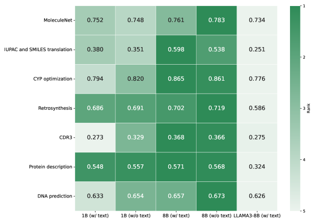
Figure 22: Ablation study results. NatureLM models are denoted as “(w/ text)”. The NatureLM models without text instruction data for post-training are denoted as “(w/o text)”. Additionally, we fine-tuned the original Llama 3 model, denoted as “Llama 3 8B (w/ text)”. Performance metrics are displayed in the cells (larger values indicate better performance), with rank represented by the color intensity (darker colors signify higher rankings).

10.1 Impact of text-based post-training data

We investigated whether incorporating general text instruction tuning data into the post-training phase affects the performance of NatureLM. To this end, we compared the results of NatureLM pest-trained with or without the inclusion of general text-based instruction data during the post-training phase. NatureLM (1B w/o text) and NatureLM (8B w/o text) denote the models without text data for post-training. We have several observations from Fig. 22:

• For the 1B parameter models, post-training without general text-based instruction data leads to better performance on scientific tasks, as evidenced by the superior performance on 5 out of 8 tasks. This suggests that at smaller scales, including text-based instruction data may not provide benefits and could potentially dilute the model’s focus on scientific instructions due to limited model capacity.

• In contrast, for the 8B parameter models, post-training with text-based instruction data does not adversely affect performance. This indicates that the larger model has sufficient capacity to incorporate both general text-based and science-based instruction data without detrimental effects on its performance on scientific tasks.

10.2 Impact of continued pre-training on scientific data

One might wonder whether it is necessary to pre-train a foundation model on scientific data or if directly fine-tuning a large language model (LLM) with scientific instruction data suffices. To address these questions, we compared our NatureLM (8B) model, which initially continues pre-training of Llama 3 8B on scientific data before undergoing post-training with scientific instruction data, against a model that directly fine-tunes the Llama 3 8B model without the pre-training step. As shown in Fig. 22, NatureLM (8B) outperforms the directly fine-tuned Llama 3 8B across all tasks, highlighting the importance of pre-training on a scientific corpus.

11 Discussions

11.1 Summary

In this work, we developed Nature Language Model (NatureLM), a sequence-based science foundation model for scientific discovery across multiple domains. Users can interact with the model using text-based instructions to generate novel scientific entities. It supports cross-domain generation and has been demonstrated in phases of drug discovery, protein generation, RNA generation, and enables predictive capabilities for small molecules, proteins, and DNA. Among the 22 tasks tested, larger models showed better performance on 18 tasks. We believe NatureLM is a significant step towards transforming scientific discovery with foundation model approaches.

11.2 Limitations

Despite the progress of NatureLM, we have identified several limitations and are committed to addressing them in future versions:

Language Capabilities: Interacting with scientific models using human language will be an essential feature to enable scientific discoveries. Although NatureLM demonstrates general language capabilities, it achieves only a 31.8% winning rate on the AlpacaEval benchmark when compared to the original Mixtral 8x7B. To enhance this, we plan to incorporate more high-quality text data in pre-training in the future.

Few-shot Capabilities: The capability of few-shot learning is critical for a foundation model. Currently, our NatureLM does not exhibit strong few-shot capabilities. We aim to enhance this by refining our training strategies and increasing the model size.

11.3 Cross-domain applications

NatureLM is a unified model that spans multiple domains, including text, small molecules, proteins, materials, and nucleotides. One significant advantage of this multi-domain unification is that it allows for the integration of knowledge from diverse fields, enabling us to tackle important cross-domain tasks that domain-specific models cannot address. While we have already provided a few examples of cross-domain tasks, here are several more that we plan to study in the future:

1. Design of Biocompatible Materials: Developing biocompatible materials requires the simultaneous consideration of material properties and protein interactions. Examples included the Titanium Alloys and Cobalt-Chromium Alloys used in hip replacement.

2. Ribozyme and Bio-Catalyst Development: Designing effective ribozymes and bio-catalysts necessitates a detailed understanding of RNA structures, protein functions, and small molecule interactions.

3. Enabling Complex System Understanding: Systems biology aims to understand the complex interplay of various components in a system, including biomolecules such as proteins, DNA, RNA, lipids, carbohydrates, and small molecules like metabolites.

Author list

Yingce Xia^∗, Peiran Jin^∗, Shufang Xie^∗, Liang He^∗, Chuan Cao^∗,

Renqian Luo^∗, Guoqing Liu^∗, Yue Wang^∗, Zequn Liu^∗, Yuan-Jyue Chen^∗,

Zekun Guo^∗, Yeqi Bai, Pan Deng, Yaosen Min, Ziheng Lu,

Hongxia Hao, Han Yang, Jielan Li, Chang Liu, Jia Zhang,

Jianwei Zhu, Kehan Wu, Wei Zhang, Kaiyuan Gao, Qizhi Pei,

Qian Wang, Xixian Liu, Yanting Li, Houtian Zhu, Yeqing Lu,

Mingqian Ma, Zun Wang, Tian Xie, Krzysztof Maziarz, Marwin Segler,

Zhao Yang, Zilong Chen, Yu Shi, Shuxin Zheng, Lijun Wu,

Chen Hu, Peggy Dai, Tie-Yan Liu, Haiguang Liu, Tao Qin

^∗ indicates co-first authors.

Corresponding authors: Tao Qin and Yingce Xia

Contact emails: {taoqin, yingce.xia}@microsoft.com

This work was conducted in Microsoft Research AI for Science.

Appendix A Supplementary figures

Figure S6: Bar plot of the correct ratio of NatureLM (1B), NatureLM (8B) and NatureLM (8x7B) on each target.

Stable - Please produce a protein sequence that exhibits stability. - I require a stable protein sequence, kindly generate one. - Generate a protein sequence ensuring its stability. - I need a protein sequence that’s stable. Please generate it. - Create a stable protein sequence. - Produce a stable protein sequence. - Kindly generate a protein sequence with stability. - I would like you to generate a stable protein sequence. - Please create a protein sequence that ensures stability. - Make a protein sequence that is stable. Soluble - Generate a soluble protein sequence. - Produce a protein sequence that is soluble. - Create a soluble protein sequence, please. - I require a soluble protein sequence, kindly generate one. - Please produce a protein sequence that exhibits solubility. - Make a protein sequence that is soluble. - Kindly generate a protein sequence with solubility. - I need a protein sequence that’s soluble. Please generate it. - I would like you to generate a soluble protein sequence. - Please create a protein sequence that ensures solubility. Insoluble - Generate an insoluble protein sequence. - Produce a protein sequence that is not soluble. - Create an insoluble protein sequence, please. - I require an insoluble protein sequence, kindly generate one. - Please produce a protein sequence that lacks solubility. - Make a protein sequence that is not soluble. - Kindly generate a protein sequence without solubility. - I need a protein sequence that’s insoluble. Please generate it. - I would like you to generate an insoluble protein sequence. - Please create a protein sequence that ensures insolubility.

Figure S13: Prompts for conditioned generation

Instruction: Tell me about Cas9 regarding its cutting mechanism?
Response:
Cas9 is a CRISPR-associated protein that can be programmed to cut DNA at a specific location. It recognizes a short DNA sequence, called a protospacer, and cuts both strands of the DNA at that site. This DNA cutting is done using two nuclease domains, HNH and RuvC, which are repsonsible for cutting the top and bottom strands of the DNA, respectively. The HNH nuclease domain cleaves the top strand, while the RuvC nuclease domain cleaves the bottom strand. The cut made by the nuclease domains leaves the DNA with a sticky end that can ligate to another DNA molecule, such as the chromosome of the cell.
Instruction: Could you provide me the advantages and disadvantages of Cas12a, another widely used CRISPR protein?
Response:
Advantages:
1. High specificty: Cas12a has higher specificity compared to Cas 9, which reduces off-target effects.
2. Simpler PAM requirements: Cas 12a requires a simpler PAM sequence than Cas9, making it easier to target specific genomic loci.
3. Multiplexing: Cas12a can be used for multiplexing genome editing, meaning multiple genomic loci can be edited in a single reaction.
Disadvantages:
4. Lower efficiency: Cas12a is less efficient in terms of indel formation than Cas9.
5. Larger size: Cas12a is a larger protein than Cas9, which can make it harder to deliver the Cas12a system into cells.
6. Lack of donor specificity: Cas12a has a lower efficiency of HDR than Cas9, which makes it difficult to target specific nucleotides for insertion or deletion. 7. Higher toxicity: Cas12a may casue higher levels of cell death than Cas9, which could impact the overall efficiency of genome editing.
8. Differing DNA repair mechanism: Cas12a and Cas9 utilize DNA different repair mechanisms, which can lead to different outcomes when targeting specific genomic loci.
9. Less versatile: Cas12a is not as versatile as Cas9, as it can only target DNA sequences that contain a TTN PAM sequence.
10. Unclear off-target effects: Cas12a has not been fully characterized in terms of off-target effects, which could lead to unwanted changes in the genome.
11. Difficulty in designing gRNAs: Cas12 requires a longer gRNA sequence compared to Cas9, making it more difficult to design effective gRNAs.

Figure S14: Response of CRISPR gene editing.

Instruction: PD-L1, Programmed Death Ligand-1, is a protein that expressed on cancer cells. Design a peptide with 10 amino acids that binds to PD-L1.
Response: $\langle$protein$\rangle$TDEDVLQKIVKRATEDSSYTVKLSNGQTLSVTE
DSEIKKIQKFRS$\langle$/protein$\rangle$

Figure S15: Response of cancer immunotherapy.

Instruction: Could you explain Lipinski’s Rule of Five and its role in evaluating the drug-likeness of chemical compounds?
Response: Lipinski’s Rule of Five, also known as the Rule of Five, is a set ofules developed by Dr. Lipinski that outlines the physical properties of successful orally active drugs. It is a set of simple guidelines that can be used to evaluate the drug-likeness of chemical compounds. It indicates whether a chemical compound with a certain set of properties will have desirable drug-like properties and is likely to be successful as an oral drug. The fiveules that comprise Lipinski’s Rule of Five are: 1. The number of hydrogen bond donors should be limited to no more than 2. The number ofotatable bonds should be limited to no more than 3. The molecular weight should be less than 500 daltons. 4. The number of hydrogen bond acceptors should be limited to no more than 10. 5. The logD value (a logarithmic measure of a compound’s hydrophobicity) should be less than 3. The application of Lipinski’s Rule of Five has been widely adopted in the pharmaceutical industry to prioritize lead compounds for drug development. It is a tool that is used to identify potentially promising compounds and can help in the elimination of compounds with poor pharmaceutical properties.

Figure S16: Response of drug discovery.

Instruction: How do I wrap a present neatly?
NatureLM: To wrap a present neatly, start by deciding on the type of wrapping paper you want to use. Next, tear the edges of the paper to make it easier to fold. Wrap the paper around the gift and use tape to hold it in place. Fold the ends of the paper over to form a neat tuck. Finally, tie a bow around the gift to finish it off.
Mixtral: To wrap a present neatly, follow these steps: 1. Gather your supplies: wrapping paper, scissors, tape, and a ruler or measuring tape. 2. Measure the length and width of the present, and cut a piece of wrapping paper that is at least 2 inches longer and wider than the present. 3. Place the present in the center of the wrapping paper, with the bottom of the present facing up. 4. Fold one side of the wrapping paper over the present, and tape it in place. 5. Fold the other side of the wrapping paper over the present, and tape it in place. 6. Fold the top and bottom edges of the wrapping paper over the present, and tape them in place.7. Flip the present over, and repeat steps 4-6 on the other side. 8. Add a ribbon or bow to the top of the present for a finishing touch. Instruction: Write a captivating movie review for a recently released science fiction film, discussing its plot, characters, and special effects.
NatureLM: It’s still quite worth seeing.
Mixtral: Captivating Movie Review: ”Interstellar” ”Interstellar” is a science fiction film directed by Christopher Nolan, starring Matthew McConaughey, Anne Hathaway, and Jessica Chastain. The film follows a group of astronauts as they travel through a wormhole in search of a new home for humanity. The plot of ”Interstellar” is complex and thought-provoking, exploring themes of time, space, and the human condition. The characters are well-developed and relatable, with McConaughey delivering a powerful performance as the lead astronaut, Cooper. The special effects in ”Interstellar” are breathtaking, with stunning visuals of space and otherworldly landscapes. The film also features a haunting score by Hans Zimmer, which adds to the emotional impact of the story. Overall, ”Interstellar” is a captivating and thought-provoking film that will leave audiences pondering the mysteries of the universe long after the credits roll.

Figure S17: Response of AlpacaEval.

Appendix B Supplementary tables

	Samples	Tokens	Samples	Tokens
Data source	(by million)	(by billion)	(%)	(%)
Text	46.3	14.4	11.6	10.0
Small molecule	68.0	4.2	17.0	2.9
Protein	192.0	65.2	47.9	45.3
DNA	13.4	19.8	3.3	13.8
RNA	37.8	27.5	9.4	19.1
Material	1.1	0.02	0.3	0.014
Cross-domain	41.9	12.7	10.5	8.8
Total	400.5	143.8	100	100

Table S1: Tokens numbers and their distribution of each domain.

Model Parameters	1B	8B	8x7B
Learning Rate	1e-4	1e-4	2e-4
Batch Size (Sentences)	4096	2048	1536
Context Length (Tokens)	8192	8192	8192
GPU number (H100)	64	256	256

Table S2: Training recipe of different models.

Porperty	Value
QED	0.5, 0.6, 0.7, 0.8, 0.9, 1.0
HBA	0, 1, 2, 3, 4, 5, 6, 7, 8, 9, 10
HBD	0, 1, 2, 3, 4, 5
FSP3	0.0, 0.1, 0.2, 0.3, 0.4, 0.5, 0.6, 0.7, 0.8, 0.9, 1.0
RotBonds	0, 1, 2, 3, 4, 5, 6, 7, 8, 9, 10
TPSA	20, 40, 60, 80, 100, 120

Table S3: Input property values for property-to-molecule generation

Target	Spearman correlation
Pancreatic alpha-amylase	0.569
Large T antigen	0.572
DNA (cytosine-5)-methyltransferase 1	0.517
Chaperone protein PapD	0.739
Catechol O-methyltransferase	0.638
Glyceraldehyde-3-phosphate dehydrogenase, glycosomal	0.503
Phosphoenolpyruvate carboxykinase cytosolic	0.501
FK506-binding protein 1A	0.606
Beta-lactamase class C	0.560
OXA-48	0.680
Ubiquitin carboxyl-terminal hydrolase 7	0.764
MAP/microtubule affinity-regulating kinase 4	0.782

Table S4: Spearman correlation between docking scores and binding affinity on the selected targets for evaluation.

Basic property	QED	QED	donor	donor	LogP	LogP
Enzyme	CYP2C9	CYP3A4	CYP2C9	CYP3A4	CYP2C9	CYP3A4	Average
1B	0.352	0.357	0.501	0.497	0.276	0.280	0.377
8B	0.404	0.428	0.548	0.522	0.332	0.340	0.429
8x7B	0.429	0.427	0.515	0.501	0.355	0.347	0.429

Table S5: Joint optimization of metabolism and a basic property.

Property Name	Training samples	Testing samples
BBBP	1272	199
BACE	90677	152
LogP	8491	473
Donor	8526	478
QED	8466	476
CYP1A2	8076	103
CYP2C9	21589	199
CYP2D6	8067	165
CYP3A4	24376	171
Total	179540	2416

Table S6: Statistics of preference data used in RLHF

Appendix C Supplementary notes

C.1 Text-guided basic property optimization of small molecule compounds

We focus on optimizing the basic molecular properties in this section. The input of NatureLM includes a text command and a SMILES sequence to be optimized. We evaluate the optimization results of Quantitative Estimation of Drug-likeness (QED), LogP, and the number of hydrogen bond donors. Following DrugAssist ye2023drugassist , we curated a fine-grained procedure. An illustrative example is provided below and the example is from DrugAssist ye2023drugassist :

Example C.1.

Instruction: With a molecule represented by the SMILES string
$\langle$mol$\rangle$CC(N)=[NH+]CC(=O)N1CCC(O)(Cn2cnc3c(cnn3-c3ccc(N4CCC5(CCOCC5)CC4)cc3)c2=O)CC1$\langle$/mol$\rangle$, propose adjustments that can increase its QED value by at least 0.1 compared to the pre-optimized value to make it more drug-like.
Response:$\langle$mol$\rangle$CC(C)(C)OC(=O)N1CCC(c2ncc(-c3ccc(CC[B-](F)(F)F)cc3)cn2)CC1$\langle$/mol$\rangle$.

For QED and hydrogen bond donor property optimization, our instructions cover the following scenarios: (i) increase or decrease the property by $\delta$, where both $\delta=0$ and $\delta>0$ are considered, aiming to verify the ability of the model; (2) maintain the properties. For LogP, the instruction is to adjust the LogP value from one specified region to another.

Model	QED	#Donor	LogP
LLAMA 3 8B∗	0.62 / 0.43	0.75 / 0.43	0.84 / 0.45
NatureLM (1B)	0.58 / 0.57	0.74 / 0.58	0.63 / 0.60
NatureLM (8B)	0.65 / 0.45	0.81 / 0.44	0.80 / 0.42
NatureLM (8x7B)	0.66 / 0.48	0.80 / 0.47	0.80 / 0.47

Table S7: Comparison between the basic property optimization. In each cell, the success rate and uniqueness ratio are reported.

The results are in Table S7. Notably, as the model size of NatureLM increases, there is a marked improvement in performance metrics across all properties. For instance, NatureLM (8B) surpasses NatureLM (1B) in all categories, indicating enhanced comprehension and manipulation of molecular structures and properties as model complexity grows. Despite DrugAssist^∗ achieving the highest scores overall, our results demonstrate that by further increasing the model size and fine-tuning the training process, there is significant potential to outperform this baseline. The trend observed with the NatureLM models underscores the importance of model scale and suggests that with continued advancements in model architecture and training methodologies, even better optimization outcomes can be achieved. This validates the proficiency of NatureLM in understanding and applying the given instructions to revise molecular properties accordingly.

C.2 Supplementary information of RNA generation

Minimum free energy (MFE) calculation:

./ViennaRNA-2.7.0/src/bin/RNAfold -p --MEA ${input_file}

Usage of cmscan:

cmscan --rfam --cut_ga --nohmmonly --tblout results_tblout --fmt 2 --clanin Rfam/Rfam.clanin Rfam/Rfam.cm ${input_file}

C.3 Supplementary information for evaluation metrics

Success Rate for BBBP and CYP Optimization

For BBBP optimization, our goal is to enhance the BBBP ability of the given compounds. These compounds are selected from the test set of the BBBP dataset in MoleculeNet, and initially, none can cross the BBB. For compounds generated by our AI method, we use BioT5 to predict their ability to cross the BBB. If a compound is predicted to cross, the optimization is considered successful.

For CYP optimization, the objective is to decrease the inhibition ability. Our prediction model uses a sigmoid function in the final layer, where $0$ indicates inhibition and $1$ indicates no inhibition. For an input molecule A and output molecule B, with predicted values $p_{a}$ and $p_{B}$, if $p_{a}>p_{b}$, the optimization is deemed successful.

C.4 Shift the focus from general text to scientific sequences

Although there are certain sequence-based foundation models for scientific tasks, their main focus is on text-based tasks and scientific understanding, instead of scientific discovery, i.e., discovering new molecules, proteins, and material. In Table S8, we compare NatureLM with several sequence models.

Model	BioGPT	MolXPT
Scope	Biomedical literature	Text and SMILES
Core Capabilities	Biomedical natural language processing	SMILES understanding and generation
Representative Tasks	• Biomedical relation extraction • Biomedical question answering • Biomedical document classification	• Molecule property prediction • Text-molecule translation
Training Data	• Text only • PubMed items before 2021 • 15M paper titles and abstracts	• 67% pure text tokens • 30M paper titles and abstracts from PubMed • 30M SMILES from PubChem • 8M interleaved sequences between SMILES and text
Training Strategy	Trained from scratch	Trained from scratch

Model	Galactica	NatureLM
Scope	Academic literature	Broader “language of nature”
Core Capabilities	• Scientific knowledge and reasoning • Scientific writing assistance	• Scientific entity generation • Scientific entity optimization
Representative Tasks	• Scientific Q&A • Citation prediction • Equation recall	• Molecule optimization • Protein-to-molecule design • Guide RNA engineering
Training Data	• More than 90% pure text tokens • Academic text (e.g., papers, knowledge bases)	• 10% pure text tokens • Diverse scientific sequences (e.g., SMILES, FASTA, DNA, RNA, material, text.)
Training Strategy	Trained from scratch	Continual pre-training on existing LLMs. Incorporates domain-specific instructions

Table S8: Comparison between existing sequence models and NatureLM.

BioGPT biogpt2022 and MolXPT liu2023molxpt are designed for the biomedical and (small) molecular domains. BioGPT is trained with titles and abstracts from PubMed items. MolXPT is trained with PubMed items as well as SMILES from PubChem. Their core capabilities are natural language tasks. Galactica galactica2022 is primarily designed for understanding and reasoning about academic literature. Its core capabilities include recalling equations, answering scientific questions, and performing domain-specific reasoning such as predicting chemical reactions and deriving mathematical proofs. It is trained on a highly curated corpus, primarily consisting of academic texts such as research papers (e.g., arXiv, PMC), reference materials, knowledge bases, LaTeX equations, and structured factual datasets. Notably, over 90% of Galactica’s training data consists of pure text, reflecting its emphasis on “academic text” and its key application in scientific writing.

In contrast, NatureLM envisions a broader “language of nature” that unifies multiple scientific domains and modalities. It is explicitly designed to process diverse sequence-based data, including small molecules (SMILES), proteins (FASTA), materials (composition, space group, and atomic coordinates), as well as DNA and RNA sequences. Unlike Galactica, which focuses on understanding and reasoning within scientific text, NatureLM focuses on generative tasks for scientific discovery, especially cross-domain generation and optimization tasks, such as protein-to-molecule design or guide RNA engineering.

Only 10% training data of NatureLM is pure text. The remaining 90% consists of scientific entities and cross-domain sequences. Furthermore, NatureLM incorporates cross-domain data where text is interlinked with SMILES, FASTA, and material representations, enabling it to span multiple scientific disciplines through sequence-based formats. This emphasis on structured scientific data allows NatureLM to bridge multiple domains and facilitates discovery-oriented tasks beyond text-based scientific reasoning.

References

- \bibcommenthead
- (1) Brown, T.B., Mann, B., Ryder, N., et. al: Language Models are Few-Shot Learners (2020). https://arxiv.org/abs/2005.14165
- (2) OpenAI, Achiam, J., et. al: GPT-4 Technical Report (2024). https://arxiv.org/abs/2303.08774
- (3) OpenAI, Hurst, A., et. al.: GPT-4o System Card (2024). https://arxiv.org/abs/2410.21276
- (4) Team, G., Anil, R., et. al: Gemini: A Family of Highly Capable Multimodal Models (2024). https://arxiv.org/abs/2312.11805
- (5) Team, G., Georgiev, P., et. al.: Gemini 1.5: Unlocking multimodal understanding across millions of tokens of context (2024). https://arxiv.org/abs/2403.05530
- (6) Abdin, M., Aneja, J., Awadalla, H., et. al: Phi-3 Technical Report: A Highly Capable Language Model Locally on Your Phone (2024). https://arxiv.org/abs/2404.14219
- (7) Abdin, M., Aneja, J., Behl, H., et. al: Phi-4 Technical Report (2024). https://www.microsoft.com/en-us/research/uploads/prod/2024/12/P4TechReport.pdf
- (8) Llama Team, A.a.M.: The Llama 3 Herd of Models (2024). https://arxiv.org/abs/2407.21783
- (9) Jiang, A.Q., Sablayrolles, A., Mensch, A., Bamford, C., Chaplot, D.S., de las Casas, D., Bressand, F., Lengyel, G., Lample, G., Saulnier, L., Lavaud, L.R., Lachaux, M.-A., Stock, P., Scao, T.L., Lavril, T., Wang, T., Lacroix, T., Sayed, W.E.: Mistral 7B (2023). https://arxiv.org/abs/2310.06825
- (10) Jiang, A.Q., Sablayrolles, A., Roux, A., Mensch, A., Savary, B., Bamford, C., Chaplot, D.S., de las Casas, D., Hanna, E.B., Bressand, F., Lengyel, G., Bour, G., Lample, G., Lavaud, L.R., Saulnier, L., Lachaux, M.-A., Stock, P., Subramanian, S., Yang, S., Antoniak, S., Scao, T.L., Gervet, T., Lavril, T., Wang, T., Lacroix, T., Sayed, W.E.: Mixtral of Experts (2024). https://arxiv.org/abs/2401.04088
- (11) DeepSeek-AI, et. al: DeepSeek-V3 Technical Report (2024). https://arxiv.org/abs/2412.19437
- (12) DeepSeek-AI, et. al: DeepSeek-R1: Incentivizing Reasoning Capability in LLMs via Reinforcement Learning (2025). https://arxiv.org/abs/2501.12948
- (13) Yang, A., Yang, B., Hui, B., et. al: Qwen2 Technical Report (2024). https://arxiv.org/abs/2407.10671
- (14) Qwen, Yang, A., et. al: Qwen2.5 Technical Report (2025). https://arxiv.org/abs/2412.15115
- (15) AI4Science, M.R., Quantum, M.A.: The Impact of Large Language Models on Scientific Discovery: a Preliminary Study using GPT-4 (2023). https://arxiv.org/abs/2311.07361
- (16) Madani, A., Krause, B., Greene, E.R., Subramanian, S., Mohr, B.P., Holton, J.M., Olmos, J.L., Xiong, C., Sun, Z.Z., Socher, R., Fraser, J.S., Naik, N.: Large language models generate functional protein sequences across diverse families. Nature Biotechnology 41(8), 1099–1106 (2023). https://doi.org/10.1038/s41587-022-01618-2
- (17) Hayes, T., Rao, R., Akin, H., Sofroniew, N.J., Oktay, D., Lin, Z., Verkuil, R., Tran, V.Q., Deaton, J., Wiggert, M., Badkundri, R., Shafkat, I., Gong, J., Derry, A., Molina, R.S., Thomas, N., Khan, Y., Mishra, C., Kim, C., Bartie, L.J., Nemeth, M., Hsu, P.D., Sercu, T., Candido, S., Rives, A.: Simulating 500 million years of evolution with a language model. bioRxiv (2024) https://www.biorxiv.org/content/early/2024/07/02/2024.07.01.600583.full.pdf. https://doi.org/10.1101/2024.07.01.600583
- (18) Zhou, Z., Ji, Y., Li, W., Dutta, P., Davuluri, R.V., Liu, H.: DNABERT-2: Efficient foundation model and benchmark for multi-species genomes. In: The Twelfth International Conference on Learning Representations (2024). https://openreview.net/forum?id=oMLQB4EZE1
- (19) Nguyen, E., Poli, M., Durrant, M.G., Kang, B., Katrekar, D., Li, D.B., Bartie, L.J., Thomas, A.W., King, S.H., Brixi, G., Sullivan, J., Ng, M.Y., Lewis, A., Lou, A., Ermon, S., Baccus, S.A., Hernandez-Boussard, T., Ré, C., Hsu, P.D., Hie, B.L.: Sequence modeling and design from molecular to genome scale with evo. Science 386(6723), 9336 (2024). https://doi.org/10.1126/science.ado9336
- (20) Cui, H., Wang, C., Maan, H., Pang, K., Luo, F., Duan, N., Wang, B.: scgpt: toward building a foundation model for single-cell multi-omics using generative ai. Nature Methods 21(8), 1470–1480 (2024). https://doi.org/10.1038/s41592-024-02201-0
- (21) Liu, Z., Zhang, W., Xia, Y., Wu, L., Xie, S., Qin, T., Zhang, M., Liu, T.-Y.: Molxpt: Wrapping molecules with text for generative pre-training. In: Proceedings of the 61st Annual Meeting of the Association for Computational Linguistics (Volume 2: Short Papers), pp. 1606–1616 (2023)
- (22) Segler, M.H., Kogej, T., Tyrchan, C., Waller, M.P.: Generating focused molecule libraries for drug discovery with recurrent neural networks. ACS central science 4(1), 120–131 (2018)
- (23) Chaves, J.M.Z., Wang, E., Tu, T., Vaishnav, E.D., Lee, B., Mahdavi, S.S., Semturs, C., Fleet, D., Natarajan, V., Azizi, S.: Tx-llm: A large language model for therapeutics. arXiv preprint arXiv:2406.06316 (2024)
- (24) Lv, L., Lin, Z., Li, H., Liu, Y., Cui, J., Chen, C.Y.-C., Yuan, L., Tian, Y.: ProLLaMA: A Protein Language Model for Multi-Task Protein Language Processing (2024). https://arxiv.org/abs/2402.16445
- (25) Luo, R., Sun, L., Xia, Y., Qin, T., Zhang, S., Poon, H., Liu, T.-Y.: Biogpt: generative pre-trained transformer for biomedical text generation and mining. Briefings in Bioinformatics 23(6), 409 (2022) https://academic.oup.com/bib/article-pdf/23/6/bbac409/47144271/bbac409.pdf. https://doi.org/%****␣main.bbl␣Line␣475␣****10.1093/bib/bbac409
- (26) Taylor, R., Kardas, M., Cucurull, G., Scialom, T., Hartshorn, A., Saravia, E., Poulton, A., Kerkez, V., Stojnic, R.: Galactica: A Large Language Model for Science (2022). https://arxiv.org/abs/2211.09085
- (27) Liang, Y., Zhang, R., Zhang, L., Xie, P.: DrugChat: Towards Enabling ChatGPT-Like Capabilities on Drug Molecule Graphs (2023). https://arxiv.org/abs/2309.03907
- (28) Wang, C., Fan, H., Quan, R., Yang, Y.: ProtChatGPT: Towards Understanding Proteins with Large Language Models (2024). https://arxiv.org/abs/2402.09649
- (29) Weininger, D.: Smiles, a chemical language and information system. 1. introduction to methodology and encoding rules. Journal of Chemical Information and Computer Sciences 28(1), 31–36 (1988). https://doi.org/10.1021/ci00057a005
- (30) Bond-Taylor, S., Leach, A., Long, Y., Willcocks, C.G.: Deep generative modelling: A comparative review of vaes, gans, normalizing flows, energy-based and autoregressive models. IEEE transactions on pattern analysis and machine intelligence 44(11), 7327–7347 (2021)
- (31) Yenduri, G., Ramalingam, M., Selvi, G.C., Supriya, Y., Srivastava, G., Maddikunta, P.K.R., Raj, G.D., Jhaveri, R.H., Prabadevi, B., Wang, W., et al.: Gpt (generative pre-trained transformer)–a comprehensive review on enabling technologies, potential applications, emerging challenges, and future directions. IEEE Access (2024)
- (32) Landrum, G., Tosco, P., Kelley, B., Rodriguez, R., Cosgrove, D., Vianello, R., sriniker, Gedeck, P., Jones, G., NadineSchneider, Kawashima, E., Nealschneider, D., Dalke, A., Swain, M., Cole, B., Turk, S., Savelev, A., tadhurst-cdd, Vaucher, A., Wójcikowski, M., Take, I., Scalfani, V.F., Walker, R., Ujihara, K., Probst, D., Lehtivarjo, J., Faara, H., guillaume godin, Pahl, A., Monat, J.: Rdkit/rdkit: 2024_09_5 (Q3 2024) Release. https://doi.org/10.5281/zenodo.14779836
- (33) Wang, Y.-C., Yang, W.-H., Yang, C.-S., Hou, M.-H., Tsai, C.-L., Chou, Y.-Z., Hung, M.-C., Chen, Y.: Structural basis of SARS-CoV-2 main protease inhibition by a broad-spectrum anti-coronaviral drug. Am. J. Cancer Res. 10(8), 2535–2545 (2020)
- (34) Davey, C.A., Sargent, D.F., Luger, K., Maeder, A.W., Richmond, T.J.: Solvent mediated interactions in the structure of the nucleosome core particle at 1.9Å resolution. J. Mol. Biol. 319(5), 1097–1113 (2002)
- (35) Pettersen, E.F., Goddard, T.D., Huang, C.C., Couch, G.S., Greenblatt, D.M., Meng, E.C., Ferrin, T.E.: UCSF chimera–a visualization system for exploratory research and analysis. J. Comput. Chem. 25(13), 1605–1612 (2004)
- (36) Materials Project, T.: Materials data on li2o by materials project (2020). https://doi.org/10.17188/1194803
- (37) Sung, M., Jeong, M., Choi, Y., Kim, D., Lee, J., Kang, J.: BERN2: an advanced neural biomedical named entity recognition and normalization tool. Bioinformatics 38(20), 4837–4839 (2022) https://academic.oup.com/bioinformatics/article-pdf/38/20/4837/46535173/btac598.pdf. https://doi.org/10.1093/bioinformatics/btac598
- (38) Zhu, W., Hessel, J., Awadalla, A., Gadre, S.Y., Dodge, J., Fang, A., Yu, Y., Schmidt, L., Wang, W.Y., Choi, Y.: Multimodal c4: An open, billion-scale corpus of images interleaved with text. ArXiv abs/2304.06939 (2023)
- (39) Zhan, J., Dai, J., Ye, J., Zhou, Y., Zhang, D., Liu, Z., Zhang, X., Yuan, R., Zhang, G., Li, L., Yan, H., Fu, J., Gui, T., Sun, T., Jiang, Y., Qiu, X.: Anygpt: Unified multimodal llm with discrete sequence modeling. ArXiv abs/2402.12226 (2024)
- (40) Team, C.: Chameleon: Mixed-Modal Early-Fusion Foundation Models (2024)
- (41) Soboleva, D., Al-Khateeb, F., Myers, R., Steeves, J.R., Hestness, J., Dey, N.: SlimPajama: A 627B token cleaned and deduplicated version of RedPajama. https://www.cerebras.net/blog/slimpajama-a-627b-token-cleaned-and-deduplicated-version-of-redpajama (2023). https://huggingface.co/datasets/cerebras/SlimPajama-627B
- (42) Kwon, W., Li, Z., Zhuang, S., Sheng, Y., Zheng, L., Yu, C.H., Gonzalez, J., Zhang, H., Stoica, I.: Efficient memory management for large language model serving with pagedattention. In: Proceedings of the 29th Symposium on Operating Systems Principles, pp. 611–626 (2023)
- (43) Yu, G.-I., Jeong, J.S., Kim, G.-W., Kim, S., Chun, B.-G.: Orca: A distributed serving system for Transformer-Based generative models. In: 16th USENIX Symposium on Operating Systems Design and Implementation (OSDI 22), pp. 521–538 (2022)
- (44) vllm-project: vLLM: A high-throughput and memory-efficient inference and serving engine for LLMs. Accessed: 2024-10-15 (2024). https://github.com/vllm-project/vllm
- (45) Yu, B., Baker, F.N., Chen, Z., Ning, X., Sun, H.: Llasmol: Advancing large language models for chemistry with a large-scale, comprehensive, high-quality instruction tuning dataset. arXiv preprint arXiv:2402.09391 (2024)
- (46) Anthropic: The claude 3 model family: Opus, sonnet, haiku (2024)
- (47) Rajan, K., Zielesny, A., Steinbeck, C.: Stout v2. 0: Smiles to iupac name conversion using transformer models (2024)
- (48) Xia, Y., Wu, K., Deng, P., Liu, R., Zhang, Y., Guo, H., Cui, Y., Pei, Q., Wu, L., Xie, S., Chen, S., Lu, X., Hu, S., Wu, J., Chan, C.-K., Chen, S., Zhou, L., Yu, N., Liu, H., Guo, J., Qin, T., Liu, T.-Y.: Target-aware molecule generation for drug design using a chemical language model*. bioRxiv (2024) https://www.biorxiv.org/content/early/2024/02/01/2024.01.08.574635.full.pdf. https://doi.org/10.1101/2024.01.08.574635
- (49) Guan, J., Qian, W.W., Peng, X., Su, Y., Peng, J., Ma, J.: 3d equivariant diffusion for target-aware molecule generation and affinity prediction. In: The Eleventh International Conference on Learning Representations (2023). https://openreview.net/forum?id=kJqXEPXMsE0
- (50) Peng, X., Luo, S., Guan, J., Xie, Q., Peng, J., Ma, J.: Pocket2Mol: Efficient molecular sampling based on 3D protein pockets. In: Chaudhuri, K., Jegelka, S., Song, L., Szepesvari, C., Niu, G., Sabato, S. (eds.) Proceedings of the 39th International Conference on Machine Learning. Proceedings of Machine Learning Research, vol. 162, pp. 17644–17655. PMLR, ??? (2022). https://proceedings.mlr.press/v162/peng22b.html
- (51) Tangallapally, R., Subramanian, C., Yun, M.-K., Edwards, A., Sharma, L.K., Yang, L., Creed, K., Wang, J., Jackowski, S., Rock, C.O., White, S.W., Lee, R.E.: Development of brain penetrant pyridazine pantothenate kinase activators. Journal of Medicinal Chemistry 67(16), 14432–14442 (2024). https://doi.org/10.1021/acs.jmedchem.4c01211
- (52) Tarr, J.C., Salovich, J.M., Aichinger, M., Jeon, K., Veerasamy, N., Sensintaffar, J.L., Arnhof, H., Samwer, M., Christov, P.P., Kim, K., Wunberg, T., Schweifer, N., Trapani, F., Arnold, A., Martin, F., Zhao, B., Miriyala, N., Sgubin, D., Fogarty, S., Moore, W.J., Stott, G.M., Olejniczak, E.T., Engelhardt, H., Rudolph, D., Lee, T., McConnell, D.B., Fesik, S.W.: Discovery of a myeloid cell leukemia 1 (mcl-1) inhibitor that demonstrates potent in vivo activities in mouse models of hematological and solid tumors. Journal of Medicinal Chemistry 67(16), 14370–14393 (2024). https://doi.org/10.1021/acs.jmedchem.4c01188
- (53) Mammoliti, O., Martina, S., Claes, P., Coti, G., Blanque, R., Jagerschmidt, C., Shoji, K., Borgonovi, M., De Vos, S., Marsais, F., Oste, L., Quinton, E., López-Ramos, M., Amantini, D., Brys, R., Jimenez, J.-M., Galien, R., van der Plas, S.: Discovery of glpg3667, a selective atp competitive tyrosine kinase 2 inhibitor for the treatment of autoimmune diseases. Journal of Medicinal Chemistry 67(11), 8545–8568 (2024). https://doi.org/10.1021/acs.jmedchem.4c00769
- (54) Pei, Q., Zhang, W., Zhu, J., Wu, K., Gao, K., Wu, L., Xia, Y., Yan, R.: BioT5: Enriching cross-modal integration in biology with chemical knowledge and natural language associations. In: Bouamor, H., Pino, J., Bali, K. (eds.) Proceedings of the 2023 Conference on Empirical Methods in Natural Language Processing, pp. 1102–1123. Association for Computational Linguistics, Singapore (2023). https://doi.org/10.18653/v1/2023.emnlp-main.70. https://aclanthology.org/2023.emnlp-main.70
- (55) Yang, K., Swanson, K., Jin, W., Coley, C., Eiden, P., Gao, H., Guzman-Perez, A., Hopper, T., Kelley, B., Mathea, M., et al.: Analyzing learned molecular representations for property prediction. Journal of chemical information and modeling 59(8), 3370–3388 (2019)
- (56) Corey, E.J., Wipke, W.T.: Computer-assisted design of complex organic syntheses: Pathways for molecular synthesis can be devised with a computer and equipment for graphical communication. Science 166(3902), 178–192 (1969)
- (57) Segler, M.H., Preuss, M., Waller, M.P.: Planning chemical syntheses with deep neural networks and symbolic ai. Nature 555(7698), 604–610 (2018)
- (58) Maziarz, K., Liu, G., Misztela, H., Kornev, A., Gaiński, P., Hoefling, H., Fortunato, M., Gupta, R., Segler, M.: Chimera: Accurate retrosynthesis prediction by ensembling models with diverse inductive biases. arXiv preprint arXiv:2412.05269 (2024)
- (59) Schneider, N., Stiefl, N., Landrum, G.A.: What’s what: The (nearly) definitive guide to reaction role assignment. Journal of Chemical Information and Modeling 56(12), 2336–2346 (2016). https://doi.org/10.1021/acs.jcim.6b00564. PMID: 28024398
- (60) Dai, H., Li, C., Coley, C., Dai, B., Song, L.: Retrosynthesis prediction with conditional graph logic network. Advances in Neural Information Processing Systems 32 (2019)
- (61) Maziarz, K., Tripp, A., Liu, G., Stanley, M., Xie, S., Gainski, P., Seidl, P., Segler, M.: Re-evaluating retrosynthesis algorithms with syntheseus. Faraday Discussions (2024)
- (62) Chen, S., Jung, Y.: Deep retrosynthetic reaction prediction using local reactivity and global attention. JACS Au 1(10), 1612–1620 (2021)
- (63) Zhong, Z., Song, J., Feng, Z., Liu, T., Jia, L., Yao, S., Wu, M., Hou, T., Song, M.: Root-aligned smiles: a tight representation for chemical reaction prediction. Chemical Science 13(31), 9023–9034 (2022). https://doi.org/10.1039/d2sc02763a
- (64) Han, Y.e.a.: Retrosynthesis prediction with an iterative string editing model. nature communications (2024)
- (65) Mariani, V., Biasini, M., Barbato, A., Schwede, T.: lDDT: a local superposition-free score for comparing protein structures and models using distance difference tests. Bioinformatics 29(21), 2722–2728 (2013)
- (66) Wu, R., Ding, F., Wang, R., Shen, R., Zhang, X., Luo, S., Su, C., Wu, Z., Xie, Q., Berger, B., Ma, J., Peng, J.: High-resolution de novo structure prediction from primary sequence. bioRxiv (2022). https://doi.org/10.1101/2022.07.21.500999
- (67) He, L., Jin, P., Min, Y., Xie, S., Wu, L., Qin, T., Liang, X., Gao, K., Jiang, Y., Liu, T.-Y.: SFM-Protein: Integrative Co-evolutionary Pre-training for Advanced Protein Sequence Representation. arXiv preprint arXiv:2410.24022 (2024)
- (68) Adolf-Bryfogle, J., Kalyuzhniy, O., Kubitz, M., Weitzner, B.D., Hu, X., Adachi, Y., Schief, W.R., Dunbrack Jr, R.L.: Rosettaantibodydesign (rabd): A general framework for computational antibody design. PLoS computational biology 14(4), 1006112 (2018)
- (69) Jin, W., Wohlwend, J., Barzilay, R., Jaakkola, T.S.: Iterative refinement graph neural network for antibody sequence-structure co-design. In: International Conference on Learning Representations (2021)
- (70) Jin, W., Barzilay, R., Jaakkola, T.: Antibody-antigen docking and design via hierarchical structure refinement. In: International Conference on Machine Learning, pp. 10217–10227 (2022). PMLR
- (71) Kong, X., Huang, W., Liu, Y.: Conditional antibody design as 3d equivariant graph translation. In: The Eleventh International Conference on Learning Representations (2022)
- (72) Gao, K., Wu, L., Zhu, J., Peng, T., Xia, Y., He, L., Xie, S., Qin, T., Liu, H., He, K., et al.: Pre-training antibody language models for antigen-specific computational antibody design. In: Proceedings of the 29th ACM SIGKDD Conference on Knowledge Discovery and Data Mining, pp. 506–517 (2023)
- (73) Yang, H., Hu, C., Zhou, Y., Liu, X., Shi, Y., Li, J., Li, G., Chen, Z., Chen, S., Zeni, C., et al.: Mattersim: A deep learning atomistic model across elements, temperatures and pressures. arXiv preprint arXiv:2405.04967 (2024)
- (74) Xie, T., Fu, X., Ganea, O.-E., Barzilay, R., Jaakkola, T.S.: Crystal diffusion variational autoencoder for periodic material generation. In: International Conference on Learning Representations (2022). https://openreview.net/forum?id=03RLpj-tc_
- (75) Zeni, C., Pinsler, R., Zügner, D., Fowler, A., Horton, M., Fu, X., Shysheya, S., Crabbé, J., Sun, L., Smith, J., et al.: Mattergen: a generative model for inorganic materials design. arXiv preprint arXiv:2312.03687 (2023)
- (76) Miller, B.K., Chen, R.T., Sriram, A., Wood, B.M.: Flowmm: Generating materials with riemannian flow matching. arXiv preprint arXiv:2406.04713 (2024)
- (77) Gruver, N., Sriram, A., Madotto, A., Wilson, A.G., Zitnick, C.L., Ulissi, Z.: Fine-Tuned Language Models Generate Stable Inorganic Materials as Text (2024). https://arxiv.org/abs/2402.04379
- (78) Antunes, L.M., Butler, K.T., Grau-Crespo, R.: Crystal structure generation with autoregressive large language modeling. Nature Communications 15(1), 10570 (2024). https://doi.org/10.1038/s41467-024-54639-7
- (79) Jain, A., Ong, S.P., Hautier, G., Chen, W., Richards, W.D., Dacek, S., Cholia, S., Gunter, D., Skinner, D., Ceder, G., Persson, K.A.: Commentary: The Materials Project: A materials genome approach to accelerating materials innovation. APL Materials 1(1), 011002 (2013) https://pubs.aip.org/aip/apm/article-pdf/doi/10.1063/1.4812323/13163869/011002_1_online.pdf. https://doi.org/10.1063/1.4812323
- (80) Scheidgen, M., Himanen, L., Ladines, A.N., Sikter, D., Nakhaee, M., Fekete, A., Chang, T., Golparvar, A., Márquez, J.A., Brockhauser, S., Brückner, S., Ghiringhelli, L.M., Dietrich, F., Lehmberg, D., Denell, T., Albino, A., Näsström, H., Shabih, S., Dobener, F., Kühbach, M., Mozumder, R., Rudzinski, J.F., Daelman, N., Pizarro, J.M., Kuban, M., Salazar, C., Ondračka, P., Bungartz, H.-J., Draxl, C.: Nomad: A distributed web-based platform for managing materials science research data. Journal of Open Source Software 8(90), 5388 (2023). https://doi.org/10.21105/joss.05388
- (81) Saal, J.E., Kirklin, S., Aykol, M., Meredig, B., Wolverton, C.: Materials design and discovery with high-throughput density functional theory: The open quantum materials database (oqmd). JOM 65(11), 1501–1509 (2013). https://doi.org/10.1007/s11837-013-0755-4
- (82) Kirklin, S., Saal, J.E., Meredig, B., Thompson, A., Doak, J.W., Aykol, M., Rühl, S., Wolverton, C.: The open quantum materials database (oqmd): assessing the accuracy of dft formation energies. npj Computational Materials 1(1), 15010 (2015). https://doi.org/10.1038/npjcompumats.2015.10
- (83) Jiao, R., Huang, W., Lin, P., Han, J., Chen, P., Lu, Y., Liu, Y.: Crystal structure prediction by joint equivariant diffusion. Advances in Neural Information Processing Systems 36 (2024)
- (84) Lorenz, R., Bernhart, S.H., Höner zu Siederdissen, C., Tafer, H., Flamm, C., Stadler, P.F., Hofacker, I.L.: Viennarna package 2.0. Algorithms for Molecular Biology 6(1), 26 (2011). https://doi.org/10.1186/1748-7188-6-26
- (85) Kalvari, I., Nawrocki, E.P., Ontiveros-Palacios, N., Argasinska, J., Lamkiewicz, K., Marz, M., Griffiths-Jones, S., Toffano-Nioche, C., Gautheret, D., Weinberg, Z., Rivas, E., Eddy, S.R., Finn, R., Bateman, A., Petrov, A.I.: Rfam 14: expanded coverage of metagenomic, viral and microrna families. Nucleic Acids Research 49(D1), 192–200 (2020) https://academic.oup.com/nar/article-pdf/49/D1/D192/35364695/gkaa1047.pdf. https://doi.org/10.1093/nar/gkaa1047
- (86) Nawrocki, E.P., Eddy, S.R.: Infernal 1.1: 100-fold faster rna homology searches. Bioinformatics 29(22), 2933–2935 (2013) https://academic.oup.com/bioinformatics/article-pdf/29/22/2933/48897722/bioinformatics_29_22_2933.pdf. https://doi.org/10.1093/bioinformatics/btt509
- (87) Xu, Y., Zhu, J., Huang, W., Xu, K., Yang, R., Zhang, Q.C., Sun, L.: Prismnet: predicting protein–rna interaction using in vivo rna structural information. Nucleic Acids Research 51(W1), 468–477 (2023)
- (88) Wu, Z., Ramsundar, B., Feinberg, E.N., Gomes, J., Geniesse, C., Pappu, A.S., Leswing, K., Pande, V.: Moleculenet: a benchmark for molecular machine learning. Chemical Science 9, 513–530 (2018). https://doi.org/10.1039/C7SC02664A
- (89) Zhu, J., Xia, Y., Wu, L., Xie, S., Zhou, W., Qin, T., Li, H., Liu, T.-Y.: Dual-view molecular pre-training. In: Proceedings of the 29th ACM SIGKDD Conference on Knowledge Discovery and Data Mining. KDD ’23, pp. 3615–3627. Association for Computing Machinery, New York, NY, USA (2023). https://doi.org/10.1145/3580305.3599317
- (90) Xu, M., Zhang, Z., Lu, J., Zhu, Z., Zhang, Y., Chang, M., Liu, R., Tang, J.: Peer: a comprehensive and multi-task benchmark for protein sequence understanding. Advances in Neural Information Processing Systems 35, 35156–35173 (2022)
- (91) Dalla-Torre, H., Gonzalez, L., Mendoza-Revilla, J., Carranza, N.L., Grzywaczewski, A.H., Oteri, F., Dallago, C., Trop, E., de Almeida, B.P., Sirelkhatim, H., et al.: The nucleotide transformer: Building and evaluating robust foundation models for human genomics. BioRxiv, 2023–01 (2023)
- (92) Zhou, Z., Ji, Y., Li, W., Dutta, P., Davuluri, R., Liu, H.: Dnabert-2: Efficient foundation model and benchmark for multi-species genome. arXiv preprint arXiv:2306.15006 (2023)
- (93) Rafailov, R., Sharma, A., Mitchell, E., Manning, C.D., Ermon, S., Finn, C.: Direct preference optimization: Your language model is secretly a reward model. Advances in Neural Information Processing Systems 36 (2024)
- (94) Mayfield, J., Lowe, D., Sayle, R.: Pistachio: Search and faceting of large reaction databases. In: ABSTRACTS OF PAPERS OF THE AMERICAN CHEMICAL SOCIETY, vol. 254 (2017). AMER CHEMICAL SOC 1155 16TH ST, NW, WASHINGTON, DC 20036 USA
- (95) Dunn, A., Wang, Q., Ganose, A., Dopp, D., Jain, A.: Benchmarking materials property prediction methods: The matbench test set and automatminer reference algorithm. npj Computational Materials 6, 138 (2020). https://doi.org/10.1038/s41524-020-00406-3
- (96) Xie, T., Wan, Y., Huang, W., Yin, Z., Liu, Y., Wang, S., Linghu, Q., Kit, C., Grazian, C., Zhang, W., et al.: Darwin series: Domain specific large language models for natural science. arXiv preprint arXiv:2308.13565 (2023)
- (97) Jablonka, K.M., Schwaller, P., Ortega-Guerrero, A., Smit, B.: Is GPT-3 all you need for low-data discovery in chemistry. ChemRxiv (2023). https://doi.org/10.26434/chemrxiv-2023-fw8n4
- (98) Breuck, P.-P.D., Evans, M.L., Rignanese, G.-M.: Robust model benchmarking and bias-imbalance in data-driven materials science: a case study on MODNet. Journal of Physics: Condensed Matter 33(40), 404002 (2021). https://doi.org/10.1088/1361-648x/ac1280
- (99) Wang, A.Y.-T., Kauwe, S.K., Murdock, R.J., Sparks, T.D.: Compositionally restricted attention-based network for materials property predictions. npj Computational Materials 7(1), 77 (2021). https://doi.org/10.1038/s41524-021-00545-1
- (100) Eriksson, D., Jankowiak, M.: High-dimensional bayesian optimization with sparse axis-aligned subspaces. arXiv:2103.00349 [cs, stat] (2021) arXiv:2103.00349 [cs, stat]
- (101) Dubois, Y., Galambosi, B., Liang, P., Hashimoto, T.B.: Length-controlled alpacaeval: A simple way to debias automatic evaluators. arXiv preprint arXiv:2404.04475 (2024)
- (102) Ye, G., Cai, X., Lai, H., Wang, X., Huang, J., Wang, L., Liu, W., Zeng, X.: Drugassist: A large language model for molecule optimization. arXiv preprint arXiv:2401.10334 (2023)
- (103) Luo, R., Sun, L., Xia, Y., Qin, T., Zhang, S., Poon, H., Liu, T.-Y.: Biogpt: generative pre-trained transformer for biomedical text generation and mining. Briefings in Bioinformatics 23(6), 409 (2022) https://academic.oup.com/bib/article-pdf/23/6/bbac409/47144271/bbac409.pdf. https://doi.org/10.1093/bib/bbac409