Entanglement and energy transportation in the central-spin quantum battery
Abstract
Quantum battery exploits the principle of quantum mechanics to transport and store energy. We study the energy transportation of the central-spin quantum battery, which is composed of spins serving as the battery cells, and surrounded by spins serving as the charger cells. We apply the invariant subspace method to solve the dynamics of the central-spin battery with a large number of spins. We establish a universal inverse relationship between the battery capacity and the battery-charger entanglement, which persists in any size of the battery and charger cells. Moreover, we find that when , the central-spin battery has the optimal energy transportation, corresponding to the minimal battery-charger entanglement. Surprisingly, the central-spin battery has a uniform energy transportation behaviors in certain battery-charger scales. Our results reveal a nonmonotonic relationship between the battery-charger size and the energy transportation efficiency, which may provide more insights on designing other types of quantum batteries.
Keywords: central-spin quantum battery, energy transportation, entanglement
PACS: 03.65. - w, 05.70. - a, 03.67.Bg,
I Introduction
Quantum technology has demonstrated promising advantages in various of fields, including computing, communication, and simulation.Nielsen ; Bennett93 ; Gisin02 ; Ladd10 ; Reiher17 ; Rudinger22 ; Duan01 Quantum resources, such as coherence and entanglement, are essential in many quantum protocols as well as simulating the physical models.Koepsell21 ; Muniz20 ; Blatt12 ; Tamura20 ; Niu21 ; Guo21 For example, quantum resources provide substantial benefits in energy manipulation, namely the quantum battery.Campisi11 ; Yang23 ; shi20 ; Ji22 ; Dou22 ; Dou22A ; Wang20 ; Lu21 ; Uzdin15 ; F13 ; Alicki13 ; Barrios17 ; Altintas14 ; Park13 ; Seah21 ; Manzano18 ; Goold16 ; Strasberg17 ; Watanabe17 ; Zhang19 Quantum battery based on the organic microcavity has been realized in experiments, showing great advantages on energy transportation.Quach22
The primary goal of quantum battery research is to explore how to increase the energy storage capacity and/or maximize the speed of charging.Ferrar18 ; Fusco16 ; Binder15 ; Andolina18 ; Santos21 ; Rossini20 ; Yu23 ; Yang231 For example, the quantum battery has the maximal stored energy in the steady state if the battery and the charger have the same coupling strength with a shared common bath.Yao21 The Dicke quantum battery (based on the Dicke model) with battery cells can achieve a superextensive charging rates, namely the charging power , for different initial states.Andolina19 The fast-charging advantage for the quantum battery comes from the coherent cooperative interaction between the charger and the battery.Xiang23
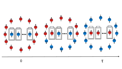
Traditional batteries use an electric field to store energy, which is then transformed into electricity by a redox process. While quantum batteries can take advantage of quantum degrees of freedom, such as spin, to store and transport energy.Jian07 ; Bortz20 Consider noninteracting spins as the battery cells and noninteracting spins as the charger cells. The battery and charger spins allow interactions, which is required for charging. See Fig. 1. The above construction is called the central-spin model, or central-spin battery in our study.Gaudin76 ; Gaudin22 The central-spin model appears in various nanostructures, such as semiconductors, quantum dots, carbon nanotubes, and nitrogen-vacancy centers in diamond.Faribault19 ; Doherty13 ; JY23 ; Li20 Specifically, the hyperfine interaction between the spin of electrons in quantum dots and the spin of surrounding nuclei can be well described by the central-spin model.Schliemann02 ; Khaetskii02 ; Deng06
Previous study has clarified the charging power of the central-spin battery. When the number of chargers is less than the number of batteries, we have the charging power ; when the number of chargers is much larger than the number of batteries, we have the charging speedup, namely .Peng21 Although the central-spin battery has a charging advantage due the coherent collective interaction, the entanglement between the charger and the battery or inside the battery spins may prohibit the battery achieving the maximal energy storage.Kamin21 ; Hovhannisyan13 ; Liu21 ; Shi22 The question on how to realize the optimal energy storage in central-spin battery has never been addressed.
In this work, we aim to explore when the central-spin battery can achieve the maximal energy storage. We focus on how the size of battery and charger, namely and , influence the maximal energy storage of the central-spin battery. We also calculate the entanglement between the charger and the battery, which clarifies the role of quantum resource in quantum batteries. Although central-spin model is integrable,Gaudin76 ; Gaudin22 traditional method such as Bethe ansatz can not capture the nonequilibrium dynamics of the integrable systems. Instead, we apply a invariant subspace method, which allows us to numerically characterize the dynamics of the system with large number of spins. Moreover, we establish the analytical results when or .
The paper is organized as follows. In Sec. II, we introduce the central-spin model as well as the the invariant subspace method. In Sec. III, we analytically study the battery capacity and the battery-charger entanglement with or . In Sec. IV, we focus on the conjectured resonant condition, namely , and numerically study the battery capacity and the battery-charger entanglement. Conclusion and outlook are presented in the final section.
II Central-spin battery
Consider the central-spin battery, which has the Hamiltonian
| (1) |
composed with the battery Hamiltonian , charger Hamiltonian , and their interaction . Specifically, we have
| (2a) | ||||
| (2b) | ||||
| (2c) | ||||
Here and with are the total spin operators for the battery and charger spins respectively. Correspondingly, we have the spin ladder operators and the . The parameters and characterize the onsite energy of the battery and charger spins, corresponding to the strengths of the external magnetic field. The parameter and characterize the flip-flop interaction (spin XX-YY interaction) and the Ising-type interaction (spin ZZ interaction), respectively. Due to the flip-flop interaction, the battery spins will be excited to high-energy states at the cost of decreasing the number of spin-up charging units. The charging process is accomplished by turning on the interaction between the battery and the charger. Here is the switch function, which equals to in while zero elsewhere. The time represents the charging time. In our previous work,Liu21 it has been proved that the battery performance is best in the case of . Therefore, we only consider in this work. The charging process of the central-spin battery is shown in Fig. 1.
To maximize the energy transportation in the charging process, we set the following initial states. At time , the battery spin is prepared in the ground state, i.e., all spins are down
| (3) |
While the charger spins are all prepared in the excited states
| (4) |
with . So the total initial state is . When , the energy of the charger spins in the initial state is larger than the energy which can be filled in the battery.Liu21
Because of the flip-flop type interaction of the central-spin battery, the total spin in the direction is conserved, that is, . Therefore, we can reformulate the dynamics into the subspace with the same number of spins
| (5) |
The parameter is defined as . The state represents the equal superposition of all states with -spin up, the so-called Dicke state.Dicke54 The dimension of the subspace is , which scales linearly with the number of spins in the battery or the charger. Note that the initial state is also enclosed.
The central-spin battery Hamiltonian can be represented as a matrix in the invariant subspace basis
| (6) |
Assuming and , we have the matrix elements
| (7a) | ||||
| (7b) | ||||
Note that the diagonal terms correspond to the initial energy difference between the battery and the charger.
To evaluate the evolution operator (with ), we can diagonalize the Hamiltonian, which gives
| (8) |
with the eigenvalue matrix . Then the charging process corresponds to the evolution
| (9) |
In the invariant subspace basis, the initial state is simply with denoting the matrix transpose. We only concern the energy in the battery, therefore knowing the reduce density matrix of the battery suffices, which is given by
| (10) |
Here is the matrix elements of in the invariant subspace basis.
III Energy transportation: analytic solution
III.1 Individual charging:
First, consider the simplest case with , namely one battery spin charged by charger spins. The initial state is . The evolution state is given by
| (11) |
The battery has the reduced density matrix
| (12) |
Then the energy transported from the charger to the battery is
| (13) |
Substitute the reduced density matrix in Eq. (12) and the battery Hamiltonian in Eq. (2a), then we have
| (14) |
Obviously, if the charging process stops at , the energy transportation achieves the maximal . The one battery spin is fully charged. Note that the charging time is proportional to .
The individual charging case also suggests that we can parallel charge each battery spin with number of chargers. And all the battery spin can be fully charged. For battery spins, the total energy transport is . Although the maximal energy transportation is guaranteed in parallel charging, it does not provide any quantum advantage on charging speedup.Xiang23 We focus on collective charging in the following sections.
III.2 Collective charging:
Suppose that the charger spins is outnumbered the battery spins, namely . If , the invariant subspace is spanned by the basis . Then the Hamiltonian is simply a matrix in such basis, given by
| (15) |
Then we can analytically solve the eigenproblem. The Hamiltonian has the eigenvalues
| (16) | ||||
| (17) | ||||
| (18) |
And the corresponding transformation matrix is
| (19) |
Then we can get the evolution state based on Eq. (9). Tracing out the charger spins, we have the density matrix of the battery spins
| (20) |
where
| (21a) | |||
with . The energy transported in the battery at time is
| (22) |
The transported energy reaches the maximal at . And the corresponding maximal transported energy is
| (23) |
Note that the battery-charger interaction strength is directly related to the optimal charging time . While the maximal transported energy is proportional to .
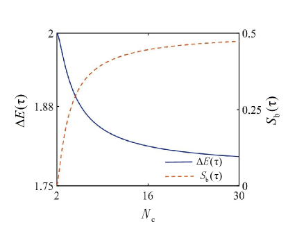
When , the battery with two spins can be fully charged, namely . However, the maximal transported energy decreases with the increasing of the charger number . See Fig. 2. Asymptotically , we have . Although increasing the number of charger spins can reduce the charging time in the collective charging, the battery can not be fully charged. We can also see that the diagonal terms (population) of the battery density matrix becomes
| (24) |
as .
As the battery is not fully charged, the density matrix of battery is a mixed state. It suggests that the battery spins are entangled with the charger spins. As demonstrated in Ref. Shi22 , the energy storage of quantum battery is limited by the battery-charger entanglement. Since the quantum state of the battery-charger system remains in a pure state over the course of time evolution, the battery-charger entanglement can be well characterized by the von Neumann entropy of the battery state (or the charger state). Specifically, the von Neumann entropy of the battery state is given by
| (25) |
which also equals to the von Neumann entropy of the charger state.
Since the battery has a pure initial state, it has a zero von Neumann entropy . For incoherent quantum batteries, entanglement is a necessary condition for generating extractable work during the charging process.Shi22 At , the battery has the maximal stored energy. We find that the corresponding von Neumann entropy of the battery state is given by
| (26) |
with the binary Shannon entropy function
| (27) |
Since is monotonic increasing with in , the von Neumann entropy increases with . See Fig. 2. Intuitively, increasing the number of charger cells would decrease the optimal charging time, which is valid in the central-spin battery. However, larger number of charger spins would generate more battery-charger entanglement, which is against the battery to be fully charged.
III.3 Collective charging:
If there are two charger spins, namely , the invariant subspace is spanned by the basis . In other words, battery spins can only be double excited, while others are remained in the ground state. In this case, the Hamiltonian can also be cast into a matrix, which is analytically tractable.
Following the similar procedure in the last subsection, we find that the transported energy is
| (28) |
where . The battery has the maximal energy at . And the corresponding transported energy is
| (29) |
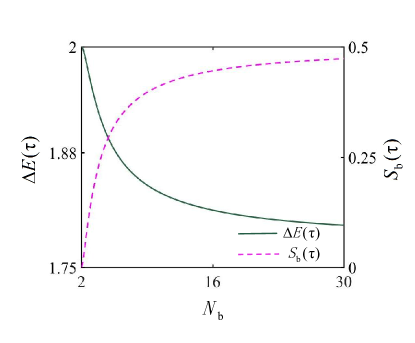
The maximal transported energy decreases with the increasing of the number of battery cells . Asymptotically , the initial charger energy can not fully transport to the battery. See Fig. 3.
We analyze the battery-charger entanglement quantified by the von Neumann entropy of the battery (charger) spins. At the optimal charging time , we have the von Neumann entropy
| (30) |
with the binary Shannon entropy function defined in Eq. (27). We can see that energy transport is negatively related with the entanglement, and the battery cells can be fully charged only at .
IV Entanglement and energy transportation: numerical analysis
IV.1 Uniform behaviors of energy transportation
In the previous section, we have established analytical results on the maximal transported energy and the battery-charger entanglement with or . Although the battery-charger entanglement is necessary during the charging process in central-spin quantum battery, any entanglement after the charging process is unwanted since it is against the battery to be fully charged.Liu21 As or , the degrees of freedom of battery or charger is dominated. Therefore, it is expected that the battery and the charger become more entangled. We conjecture that the battery has the maximal transported energy per battery cell at .
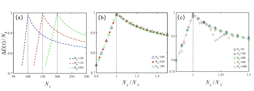
The invariant subspace method introduced in Sec. II allows us to numerically track the dynamics with larger number of spins. First, we take the number of battery cells as . Then calculate the maximal transported energy with different numbers of (by numerically finding the optimal charging time ). See Fig. 4(a). The maximal transported energy per battery cell, namely , is largest at , which is consistent with our analytical results on .
Figure 4(a) shows an interesting uniform behavior of the maximal transported energy. To give a fair comparison, we plot the maximal transported energy per battery cell in terms of the battery-charger ratio . See Fig. 4(b). In such battery scales, namely , we find that the maximal transported energy per battery cell scales almost perfectly identical.
By further increasing the battery scale, we find that the uniform characteristics is breaking. See Fig. 4(c). Oscillation appears as . The maximal transported energy may be directly related to the scale difference, namely , rather than the scale ratio . Nevertheless, the resonant condition always gives the largest transported energy in the central-spin model, which numerically verify our conjecture.
IV.2 Entanglement and energy transportation at
In Sec. III, we know that all the charger energy can transport to the battery when , which is the most economic charging protocol. Even though we know that the battery has the maximal transported energy at , it does not guarantee that all the charger energy can be completely transport to the battery.
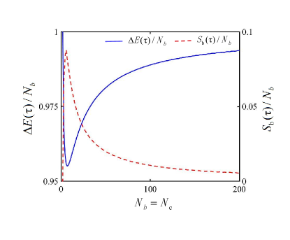
First, we study how the size of the battery cells with influence the maximal transported energy per battery cell . See Fig. 5. The perfect charging only occurs at . As the number of battery cells increases, the maximal transported energy per battery cell decreases. However, the energy transportation returns to the optimal as . We have a minimum of around . It is expected that the battery-charger entanglement behaves inversely, namely having the minimum at . Then increases with the number of battery cells. We can see that the maximal transported energy per battery cell is closely related to the battery-charger entanglement per battery cell. See Fig. 5.
Based on the above results, we propose the optimal charging protocol for the central-spin battery as follows. For small size of battery, such as , pair each two battery cells with two charger cells, then parallel charging the battery into full capacity. For relative large size of battery, pair all the battery cells with the same number of charger cells, then collectively charge the battery to the maximal, with the almost full capacity. Note that it is also worthwhile to apply the collective charging protocol as the battery size is large in the viewpoint of quantum charging speedup.
V Conclusion and outlook
In this work, we systematically analyse the energy transportation in central-spin battery. First, we obtain analytical results on the battery capacity and the battery-charger entanglement with or . The analytical results clearly show that the battery has the maximal capacity when . Therefore we conjecture that the resonant condition always gives the maximal (central-spin) battery capacity, and numerically verify it up to 2000 battery cells (spins). Second, for midsize battery, namely , we find a uniform relationship between the energy capacity (per charger cell) and the battery-charger size ratio . The uniform relation for the midsize battery also gives a tight upper bound on the energy capacity when the battery cells become large. Third, we demonstrate the universal inverse relationship between the battery capacity and the battery-charger entanglement. Since the highest excited state of the battery spin, corresponding to the maximal battery storage, is a pure state, it is expected that any battery-charger entanglement prohibits the battery to reach the maximal energy capacity. It is also consistent with general theory of quantum battery.Shi22
Charging process is a typical nonequilibrium dynamics, which is a challenging problem especially for the many-body system. The uniform behavior of the battery capacity may suggest that the conserved charges,Villazon20 ; Tang23 which are independent on the number of spins, play a role here. The resonant condition, namely , is a critical point for the central-spin battery. Whether a similar results exist in other types of quantum battery, such as the spin-chain quantum battery,Le18 Dicke quantum battery,Ferrar18 ; Dou22 ; Xiang23 and the Sachdev-Ye-Kitaev quantum battery,Rossini20 is an open problem. We leave above questions for future study.
ACKNOWLEDGMENTS
This work was supported by the NSFC (Grants No. 12275215, No. 12305028, and No. 12247103), the Major Basic Research Program of Natural Science of Shaanxi Province (Grant No. 2021JCW-19), Shaanxi Fundamental Science Research Project for Mathematics and Physics (Grant No. 22JSZ005) and the Youth Innovation Team of Shaanxi Universities.
References
- (1) Nielsen M A and Chuang I 2000 Quantum computation and quantum information (Cambridge University Press)
- (2) Bennett C H, Brassard G, Popescu S, Schumacher B, Smolin G A and Wootters W K 1996 Phys. Rev. Lett. 76 722
- (3) Gisin N, Ribordy G, Tittel W and Zbinden H 2002 Rev. Mod. Phys. 74 145
- (4) Ladd T D, Jelezko F, Laflamme R, Nakamura Y, Monroe C and O’ Brien J L 2010 Nature 465 45-53
- (5) Reiher M, Wiebe N, Svore K M, Wecker D and Troyer M 2017 Proc. Natl. Acad. Sci. U.S.A. 114 7555
- (6) Boixo S, Isakov S V, Smelyanskiy V N, Babbush R, Ding N, Jiang Z, Bremner M J, Martinis and H. Neven 2018 Nat. Phys. 14 595
- (7) Duan L M, Lukin M D, Cirac J I and Zoller P 2001 Nature(London) 414 413
- (8) Koepsell J, Bourgund D, Sompet P, Hirthe S, Bohrdt A, Wang Y, Grusdt F, Demler E, Salomon G, Gross C and Bloch 2021 Science 374 82
- (9) Muniz J A, Barberena D, Lewis-Swan R J, Young D J, Cline J R K, Rey A M and Thompson J K 2020 Nature(London) 580 602
- (10) Blatt R and Roos C F 2020 Nat. Phys. 8 277
- (11) Tamura M, Mukaiyama T and Toyoda K 2020 Phys. Rev. Lett. 124 200501
- (12) Niu J J, Yan T X, Zhou Y X, Tao Z Y, Li X L, Liu W Y, Zhang L B, Jia H, Liu S, Yan Z B, Chen Y Z, Yu D 2021 Sci Bull 66 1168
- (13) Guo Q J, Cheng C, Sun Z H, Song Z X, Li H K, Wang Z, Ren W H, Dong H, Zheng D N, Zhang Y R, Mondaini R, Fan H and Wang H 2021 Nat. Phys. 17 234
- (14) Campisi M, Hanggi P and Talkner P 2011 Rev. Mod. Phys. 83 1653
- (15) Yang X, Yang Y H, Alimuddin M, Salvia R, Fei S M, Zhao L M, Nimmrichter S and Luo M X 2023 Phys. Rev. Lett. 131 030402
- (16) Shi Y H, Shi H L, Wang X H, Hu M L, Liu S Y, Yang W L and Fan H 2020 Journal of Physics A: Mathematical and Theoretical 53 085301
- (17) Ji W, Chai Z, Wang M, Guo Y, Rong X, Shi F, Ren C L, Wang Y and Du J F 2022 Phys. Rev. Lett. 128 090602
- (18) Dou F Q, Lu Y Q, Wang Y J and Sun J A 2022 Phys. Rev. B 105 115405
- (19) Dou F Q, Zhou H and Sun J A 2022 Phys. Rev. A 106 032212
- (20) Wang Z, Li H, Feng W, Song X, Song C, Liu W, Guo Q, Zhang X, Dong H, Zheng D, Wang H and Wang D W 2022 Phys. Rev. Lett. 124 013601
- (21) Lu W, Chen J, Kuang L M and Wang X 2021 Phys. Rev. A 104 043706
- (22) Uzdin R, Levy A and Kosloff R 2015 Phys. Rev. X 5 031044
- (23) Brando F G S L, Horodecki M, Oppenheim J, Renes J M and Spekkens R W 2013 Phys. Rev. Lett. 111 250404
- (24) Alvarado Barrios G, Albarrn-Arriagada F, Crdenas-Lpez F A, Romero G and Retamal J C 2017 Phys. Rev. A 996 052119
- (25) Altintas F, Hardal A C and Mstecapliolu E 2014 Phys. Rev. E 90 032102
- (26) Park J J, Kim K H, Sagawa T and Kim S W 2017 Phys. Rev. Lett. 111 230402
- (27) Seah S, Perarnau-Llobet M, Haack G, Brunner N and Nimmrichter S 2017 Phys. Rev. Lett. 127 100601
- (28) Manzano G, Plastina F and Zambrini R 2017 Phys. Rev. Lett. 121 120602
- (29) Goold J, Huber M, Riera A, del Rio L and Skrzypczyk P 2016 J. Phys. A 49 143001
- (30) Strasberg P, Schaller G, Brandes T and Esposito M 2017 Phys. Rev. X 7 021003
- (31) Watanabe G, Venkatesh B P, Talkner P and del Campo A 2017 Phys. Rev. Lett. 118, 050601
- (32) Zhang Y Y, Yang T R, Fu L and Wang X 2019 Phys. Rev. E 99 052106
- (33) Alicki R and Fannes M 2013 Phys. Rev. E 87 042123
- (34) Quach J Q, McGhee K E, Ganzer L, Rouse D M, Lovett B W, Gauger E M, Keeling J, Cerullo G, Lidzey D G and Virgili T 2022 Sci. Adv. 8 eabk3160
- (35) Liu J X, Shi H L, Shi Y H, Wang X H and Yang W L 2021 Phys. Rev. B 104 245418
- (36) Ferraro D, Campisi M, Andolina G M, Pellegrini V and Polini M 2018 Phys. Rev. Lett. 120 117702
- (37) Fusco L, Paternostro M and Chiara G D 2016 Phys. Rev. E 94 052122
- (38) Binder F C, Vinjanampathy S, Modi K and Goold J 2015 New J. Phys. 17 075015
- (39) Andolina G M, Farina D, Mari A, Pellegrini V, Giovannetti V and Polini M 2018 Phys. Rev. B 98 205423
- (40) Santos A C 2021 Phys. Rev. E 103 042118
- (41) Rossini D, Andolina G M, Rosa D, Carrega M and Polini M 2020 Phys. Rev. Lett. 125 236402
- (42) Yu W L, Zhang Y, Li H, Wei G F, Han L P, Tian F and Zou J 2023 Chin. Phys. B 32 010302
- (43) Yang Z Q, Zhou L K, Zhou Z Y, Jin G R, Cheng L and Wang X G 2023 Chin. Phys. B 32 110301
- (44) Yao Y and Shao X Q 2021 Phys. Rev. E 104 044116
- (45) Andolina G M, Keck M, Mari A, Campisi M, Giovannetti V and Polini M 2019 Phys. Rev. Lett. 122 047702
- (46) Zhang X and Blaauboer M 2023 Front. Phys. 10 1097564
- (47) Li J and Shen S Q 2007 Phys. Rev. B 76 153302
- (48) Bortz M and Stolze J 2007 Phys. Rev. B 76 014304
- (49) Gaudin M 1976 J. Phys. 37 10
- (50) Dominguez F, Esebbag C and Dukelsky J 2006 J. Phys. A 39 11349
- (51) Faribault A, Koussir H and Mohamed M H 2019 Phys. Rev. B 100 205420
- (52) Doherty M W, Manson N B, Delaney P, Jelezko F, Wrachtrup J and Hollenberg L C L 2013 Phys. Rep. 528 1
- (53) Fan J Y and Pang S S 2023 Phys. Rev. A 107 022209
- (54) Li Z, Yang P, You W L and Wu N 2023 Phys. Rev. A 102 032409
- (55) Schliemann J, Khaetskii A V and Loss D 2002 Phys. Rev. B 66 245304
- (56) Alexander V. Khaetskii, Loss D and Glazman L 2002 Phys. Rev. Lett. 88 186802.
- (57) Deng C and Hu X 2006 Phys. Rev. B 73 241303
- (58) Peng L, He W B, Chesi S, Lin H Q and Guan X W 2021 Phys. Rev. A 103 052220
- (59) Kamin F H, Tabesh F T, Salimi S and Santos A C 2020 Phys. Rev. E 102 052109
- (60) Hovhannisyan K V, Perarnau-Llobet M, Huber M and Acin A 2013 Phys. Rev. Lett. 111 240401
- (61) Shi H L, Ding S, Wan Q K, Wang X H and Yang W L 2022 Phys. Rev. Lett. 129 130602
- (62) Dicke R H, 1954 Phys. Rev. 93 99
- (63) Villazon T, Chandran A and Claeys P W 2020 Phys. Rev. R 2 032052
- (64) Tang L H, Long D M, Polkovnikov A, Chandran A and Claeys P W 2023 Scipost Phys. 15 030
- (65) Le T, Levinsen J, Modi K, Parish M M and Pollock F A 2018 Phys. Rev. A 97 022106