Abstract

We propose a new approach for unsupervised alignment of heterogeneous datasets, which maps data from two different domains without any known correspondences to a common metric space. Our method is based on an unbalanced optimal transport problem with Gromov–Wasserstein marginal penalization. It can be seen as a counterpart to the recently introduced joint multidimensional scaling method. We prove that there exists a minimizer of our functional and that for penalization parameters going to infinity, the corresponding sequence of minimizers converges to a minimizer of the so-called embedded Wasserstein distance. Our model can be reformulated as a quadratic, multi-marginal, unbalanced optimal transport problem, for which a bi-convex relaxation admits a numerical solver via block-coordinate descent. We provide numerical examples for joint embeddings in Euclidean as well as non-Euclidean spaces.

1 Introduction

The comparison of heterogeneous data distributions is a fundamental task in computer vision, computational biology and machine learning. Most existing approaches rely on using a suitable ground cost function such as an available metric. A classic example is the Wasserstein distance which seeks an optimal transport (OT) between two given distributions. However, often the given distributions are in heterogeneous spaces, where a readily available ground cost function between these spaces does not generally exist. Additional effort may be required to learn appropriate cost functions Cuturi & Avis (2014); Heitz et al. (2021). However, even if there exists a natural embedding into a canonical joint metric space, this metric may not be suited to accurately gauge differences in their samples. Examples of such heterogeneous settings are, e.g., the comparison of graph- or mesh-valued data such as 3d shapes or manifolds. This paper introduces a novel framework based on OT which enables the joint comparison and visualization of heterogeneous datasets by optimally transferring them into an a-priori fixed metric space, see Figure 3 for an illustrative example.

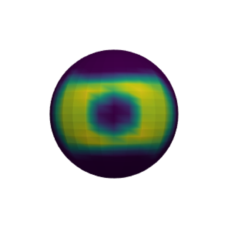
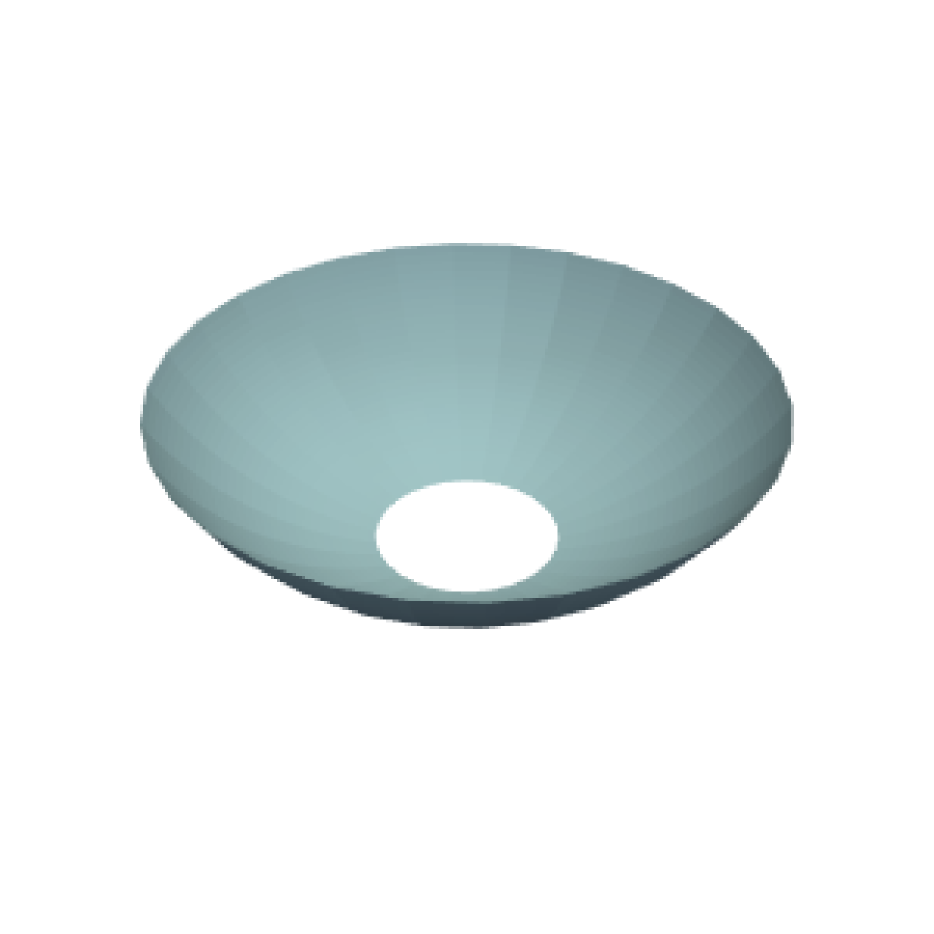
Original

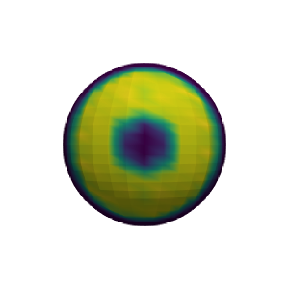
Aligned

(a) Spherical embedding

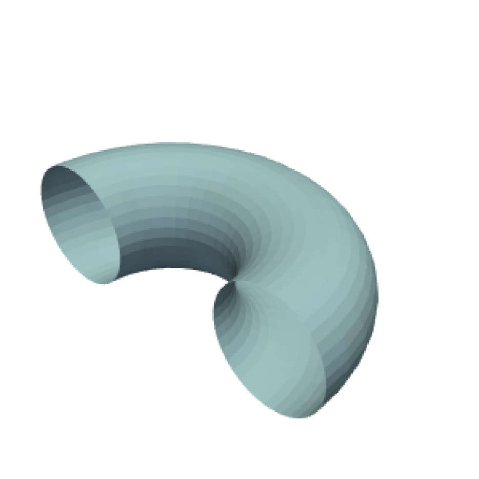
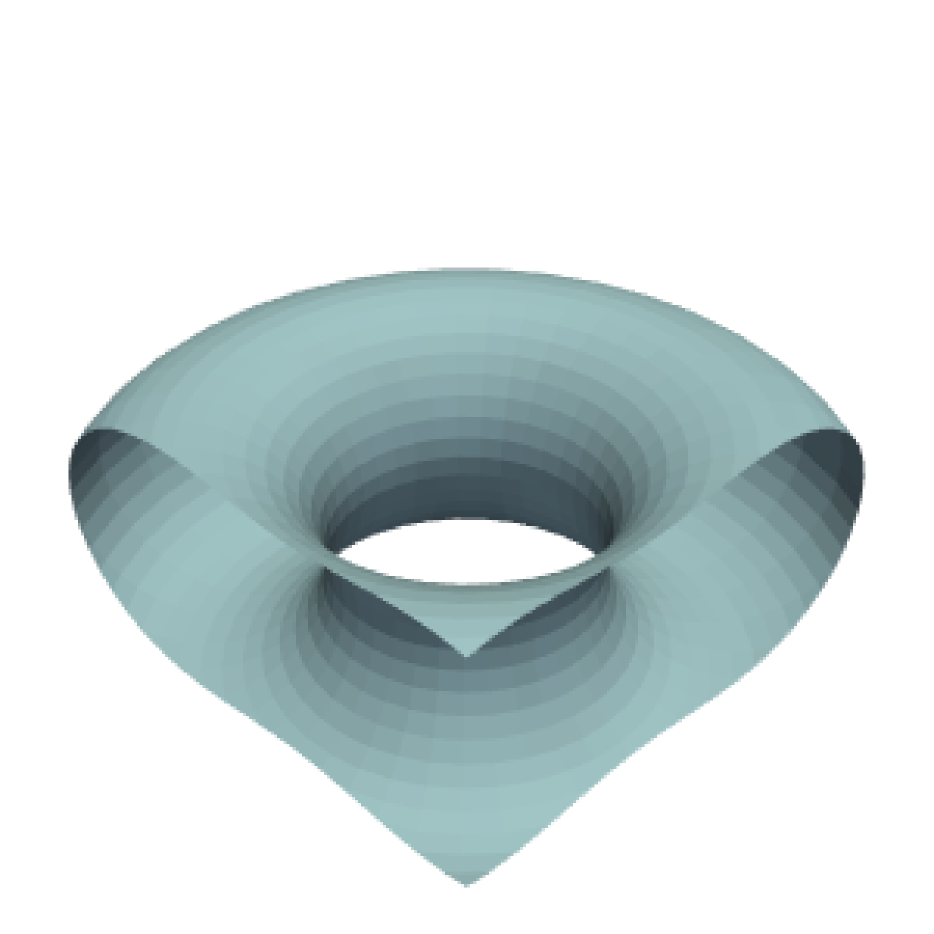
Original

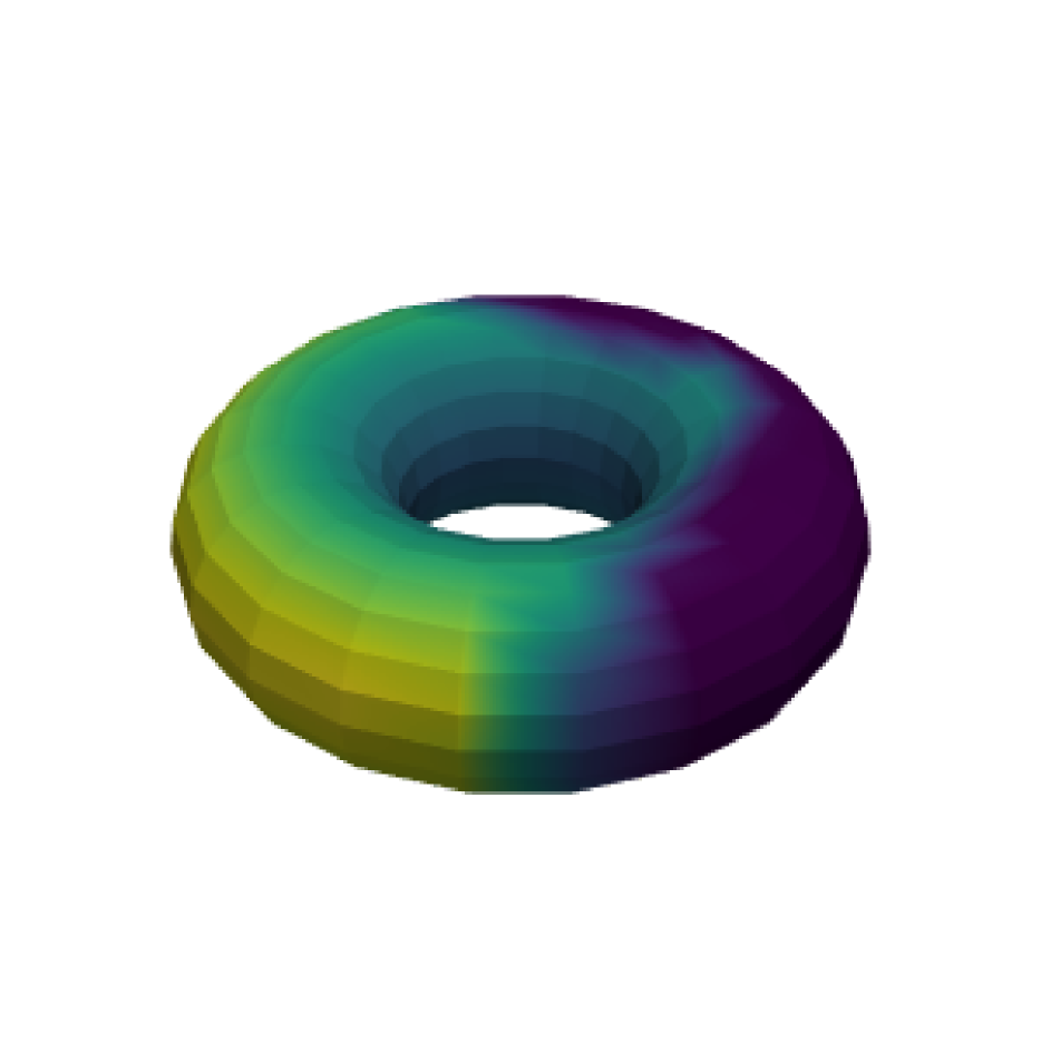
Aligned

(b) Toroidal embedding

Figure 3: Joint (aligning) transfer of two metric spaces (gray surfaces with surface distance) to a fixed reference space, namely to the sphere and the torus by our method, where the color “yellow” corresponds to higher values, see Subsection 6.1.

1.1 Previous Work

As a first step, we highlight the most relevant contributions related to our study among the vast literature on OT and dimensionality reduction.
Optimal Transport with Invariances. Optimal transport and Wasserstein distances enable comparisons of point clouds in metric spaces. However, classic OT lacks invariance to important transformations like rotations in Euclidean space. To address this, Gromov–Wasserstein (GW) distances are introduced which allow for the comparison of measures from distinct metric spaces Mémoli (2011); Sturm (2006). In Alaya et al. (2022), an approximation of GW distances is obtained by jointly embedding measures into Euclidean spaces. Furthermore, projection- and subspace-robust Wasserstein-2 distances are introduced in Paty & Cuturi (2019). Another approach incorporates invariance to Euclidean isometries via the Wasserstein Procrustes problem Grave et al. (2019). This is extended to account for linear operators with bounded Schatten norms in Alvarez-Melis et al. (2019) and to Gaussian mixture applications in Salmona et al. (2024). As outlined in Section 5, our paper extends such invariant OT to non-Euclidean domains.
Joint Dimensionality Reduction. Dimensionality reduction is a core topic in machine learning enabling visualization and clustering by finding optimal low-dimensional representations of data. Classical methods like principal component analysis (PCA) Greenacre et al. (2022) and multidimensional scaling (MDS) Carroll & Arabie (1998) preserve large variations or pairwise distances, but fail on nonlinear manifolds Alaya et al. (2022); Deng et al. (2024). Nonlinear approaches, e.g., locally linear embedding Roweis & Saul (2000), probabilistic models, e.g., t-distributed stochastic neighbor embedding (t-SNE) Van der Maaten & Hinton (2008), and deep learning methods, e.g., variational autoencoders (VAEs), Kingma et al. (2019) address these challenges. As an extension, several recent methods focus on joint embeddings of heterogeneous data. Here, we are given data on two incompatible domains and are interested in simultaneous embedding. The manifold-aligning generative adversarial network Amodio & Krishnaswamy (2018) employs a generative adversarial network for domain alignment. Maximum mean discrepancy (MMD) manifold-alignment Liu et al. (2019) balances an MMD and a distortion term. UnionCom Cao et al. (2020) leverages the generalized unsupervised manifold alignment (GUMA) Cui et al. (2014). Single-cell alignment with optimal transport (SCOT) Demetci et al. (2022) and the partial manifold alignment algorithm Cao et al. (2022) employ GW distances. Finally, the recently proposed joint multidimensional scaling (JMDS) Chen et al. (2023) algorithm combines MDS with OT for the joint embedding of two datasets into a shared Euclidean space. Complementing this and the work on non-Euclidean embeddings in McInnes et al. (2018); Deng et al. (2024), we propose a joint embedding into arbitrary metric spaces based on GW distances.

1.2 Contribution

Our main contributions are the following:
1. Towards the aligned “embedding” of heterogeneous metric spaces into a fixed, not necessarily Euclidean space, we propose to minimize an unbalanced OT problem with a quadratic cost function, where the marginals are penalized by GW distances. This formulation seeks near-isometric joint embeddings of the inputs into a metric space, while enabling an optimal comparison in the Wasserstein distance.
2. We prove that our functional has a minimizer. Further, if its regularization parameter goes to infinity, our functional approaches the so-called “embedded Wasserstein distance” Salmona et al. (2024). In this sense, we also refer to our model as the “relaxed embedded Wasserstein distance”.
3. For the (approximate) computation of a minimizer, we provide an equivalent formulation of our model as a quadratic, multi-marginal, unbalanced OT problem. A bi-convex relaxation enables the application of existing algorithms to solve the problem numerically.
4. We recall JMDS from the point of view of our model: while we are searching for the weight of atomic measures fixing their supports, JMDS fixes the weights and aims to find the supports of the measures.
5. Numerical experiments demonstrate the potential of our method for joint embeddings of heterogeneous data on the 2d Euclidean space, the torus, the 2-sphere and the space of 2d Gaussians with the Wasserstein distance.

All proofs are given in Appendix A.

2 OT-Based Distances

Given a compact metric space $(Z,d_{Z})$, we denote by $\mathcal{P}(Z)$ the space of probability measures defined on the Borel-$\sigma$-algebra induced by the distance $d_{Z}$. For two compact metric spaces $Z_{1}$ and $Z_{2}$, the push-forward measure of $\mu\in\mathcal{P}(Z_{1})$ under a measurable map $T\colon Z_{1}\to Z_{2}$ is denoted by $T_{\sharp}\mu\coloneqq\mu\circ T^{-1}\in\mathcal{P}(Z_{2})$. The set of transport plans between two measures $\mu_{1}\in\mathcal{P}(Z_{1})$ and $\mu_{2}\in\mathcal{P}(Z_{2})$ is given by

$$\Pi(\mu_{1},\mu_{2})\coloneqq\bigl{\{}\pi\in\mathcal{P}(Z_{1}\times Z_{2}):P_{i,\sharp}\pi=\mu_{i},\;i=1,2\bigr{\}},$$ (1)

where $P_{i}\colon Z_{1}\times Z_{2}\to Z_{i},(z_{1},z_{2})\mapsto z_{i}$, $i=1,2$, denotes the projection to the first and second component, respectively.

To lift $d_{Z}$ from $Z$ to $\mathcal{P}(Z)$, we rely on the Wasserstein(-2) distance between $\mu_{1},\mu_{2}\in\mathcal{P}(Z)$ defined by

$$\operatorname{W}(\mu_{1},\mu_{2})\coloneqq\!\!\min_{\pi\in\Pi(\mu_{1},\mu_{2})}\Bigl{(}\!\int\limits_{Z\times Z}d_{Z}^{2}(z,z^{\prime})\,\mathrm{d}\pi(z,z^{\prime})\!\Bigr{)}^{\frac{1}{2}}.$$ (2)

By $\Pi_{\mathrm{o}}(\mu_{1},\mu_{2})$, we denote the set of minimizers in (2). The Wasserstein distance metricizes the weak convergence of measures, where a sequence of measures $(\mu_{n})_{n\in\mathbb{N}}$ converges weakly to a measure $\mu\in\mathcal{P}(Z)$, written $\mu_{n}\rightharpoonup\mu$, if for every (bounded) continuous function $\varphi\colon Z\to\mathbb{R}$, we have $\int_{Z}\varphi\,\mathrm{d}\mu_{n}\to\int_{Z}\varphi\,\mathrm{d}\mu$ as $n\to\infty$.

To compare heterogeneous data via their internal geometry, we can rely on GW distances, which enables us to compare measures on different metric spaces. To highlight the connection between measures and underlying spaces, we consider metric measure spaces (mm-spaces), which are triples $\mathbb{X}=(X,d_{X},\xi)$ such that $(X,d_{X})$ is a compact metric space and $\xi\in\mathcal{P}(X)$. Two mm-spaces $\mathbb{X}_{i}=(X_{i},d_{X_{i}},\xi_{i})$, $i=1,2$, are isomorphic if there exists a bijective map $I\colon\operatorname*{supp}\xi_{1}\to\operatorname*{supp}\xi_{2}$ between the supports of the measures such that $I$ is measure-preserving, i.e., $I_{\sharp}\xi_{1}=\xi_{2}$, and $I$ is an isometry, i.e., $d_{X_{1}}(x_{1},x_{1}^{\prime})=d_{X_{2}}(I(x_{1}),I(x_{1}^{\prime}))$ for all $x_{1},x_{1}^{\prime}\in\operatorname*{supp}\xi_{1}$. By $[\mathbb{X}]$ we denote the equivalence class of all mm-spaces which are isomorphic to $\mathbb{X}$. Finally, if $I$ is an isometry between two metric spaces $X_{i}$, $i=1,2$, we write $I\colon X_{1}\hookrightarrow X_{2}$, and just $X_{1}\hookrightarrow X_{2}$ if such an isometry between $X_{1}$ and $X_{2}$ exists.

Sturm’s GW distance Sturm (2006) between two mm-spaces $\mathbb{X}_{i}$, $i=1,2$, is defined by

$$\operatorname{SGW}(\mathbb{X}_{1},\mathbb{X}_{2})\coloneqq\!\inf\limits_{\begin{subarray}{c}(Z,d_{Z})\text{ metric space},\\ I_{i}\colon\operatorname*{supp}\xi_{i}\hookrightarrow Z,\,i=1,2\end{subarray}}\!\operatorname{W}(I_{1,\sharp}\xi_{1},I_{2,\sharp}\xi_{2}),$$

where the Wasserstein distance is taken over the respective space $(Z,d_{Z})$. The SGW distance seeks optimal isometric embeddings of either mm-space into a joint metric space such that their Wasserstein distance in the embedded space is minimal, see Figure 4(a). Indeed, SGW is a metric on the equivalence classes of mm-spaces.

Mémoli proposed a different GW distance, which is numerically more appealing than Sturm’s construction. For two mm-spaces $\mathbb{X}_{i}$, $i=1,2$, Mémoli’s GW distance Mémoli (2011) is defined by

$$\operatorname{GW}(\mathbb{X}_{1},\mathbb{X}_{2})\coloneqq\min_{\gamma\in\Pi(\xi_{1},\xi_{2})}G_{X_{1},X_{2}}(\gamma)^{\frac{1}{2}}$$ (3)

with the quadratic GW objective

$$G_{X_{1},X_{2}}(\gamma) \coloneqq\iint\limits_{(X_{1}\times X_{2})^{2}}\bigl{(}d_{X_{1}}(x_{1},x_{1}^{\prime})-d_{X_{2}}(x_{2},x_{2}^{\prime})\bigr{)}^{2}$$ (4)

$$\hskip 27.0pt{\times}\,\mathrm{d}\gamma(x_{1},x_{2})\,\mathrm{d}\gamma(x_{1}^{\prime},x_{2}^{\prime}).$$ (5)

The problem seeks a transport between $\mathbb{X}_{1}$ and $\mathbb{X}_{2}$ which minimizes the overall pairwise distance distortion, see Figure 4(b). Both distances—SGW and GW— define a metric on the equivalence classes of mm-spaces. Furthermore, both distances induce the same topology, but SGW turns these equivalence classes into a complete metric space, while GW does not Sturm (2006); Mémoli (2011). The later can be alleviated by embedding into a larger space and extending the GW definition accordingly Sturm (2023).

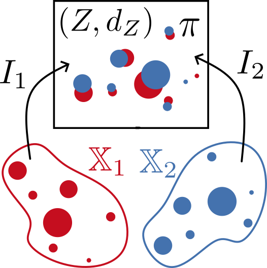
(a) Sturm’s GW

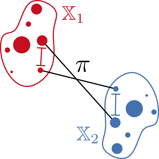
(b) Mémoli’s GW

Figure 4: Illustration of GW formulations of Sturm and Mémoli.

3 Unbalanced OT With GW Penalization

Throughout this section, let $(Z,d_{Z})$ be a fixed compact metric space. Furthermore, let $\mathbb{X}_{i}=(X_{i},d_{X_{i}},\xi_{i})$, $i=1,2$, be two mm-spaces, whose measures’ support can be isometrically embedded into $(Z,d_{Z})$, i.e., $\operatorname*{supp}\xi_{i}\hookrightarrow Z$. For this specific setting, we relax Sturm’s GW distance to

$$\operatorname{EW}(\mathbb{X}_{1},\mathbb{X}_{2})\coloneqq\inf_{\begin{subarray}{c}I_{1}\colon\operatorname*{supp}\xi_{1}\hookrightarrow Z\\ I_{2}\colon\operatorname*{supp}\xi_{2}\hookrightarrow Z\end{subarray}}\operatorname{W}(I_{1,\sharp}\xi_{1},I_{2,\sharp}\xi_{2}).$$ (6)

On a certain subspace of equivalence classes of mm-spaces, this defines a metric, which we call embedded Wasserstein metric. For the specific case of Euclidean spaces $X_{1}$, $X_{2}$, and $Z$, this reduces to the Wasserstein Procrustes problem Grave et al. (2019) and to the “embedded Wasserstein metric” in Salmona et al. (2024). We adopt this name.

Proposition 3.1.

$\operatorname{EW}$ defines a metric on the subset of isomorphic classes $[(X,d_{X},\xi)]$ for which there exist surjective isomorphism $I\colon\operatorname*{supp}\xi\hookrightarrow Z$.

By the following proposition, the infimum in (6) is attained.

Proposition 3.2.

Let $\mathbb{X}_{i}$, $i=1,2$ be two mm-spaces and $(Z,d_{Z})$ a metric space such that $\operatorname*{supp}\xi_{i}\hookrightarrow Z$ for $i=1,2$. Then the infimum in (6) is attained.

While EW relies on appropriate isometries, the following relaxation enables to handle arbitrary mm-spaces $\mathbb{X}_{i}$, $i=1,2$. For $\lambda>0$, we consider the following GW penalized unbalanced OT problem

$$\operatorname{EW}_{\lambda}(\mathbb{X}_{1},\mathbb{X}_{2}) \coloneqq\inf_{\pi\in\mathcal{P}(Z\times Z)}\!\!\Big{(}\int_{Z\times Z}d_{Z}^{2}(z,z^{\prime})\,\mathrm{d}\pi(z,z^{\prime})$$ (7)

$$+\lambda\sum_{i=1}^{2}\operatorname{GW}^{2}(\mathbb{X}_{i},(Z,d_{Z},P_{i,\sharp}\pi))\Big{)}^{\frac{1}{2}}.$$ (8)

By penalizing the GW terms, the marginals $P_{i,\sharp}\pi\in\mathcal{P}(Z)$ take a form that enforces $(Z,d_{Z},P_{i,\sharp}\pi)$ to be nearly isomorphic to the inputs $\mathbb{X}_{i}$, $i=1,2$. Furthermore, the first term ensures that the marginals $P_{i,\sharp}\pi$, $i=1,2$ are close in the Wasserstein distance on $(Z,d_{Z})$. The penalization extends EW to non-isomorphic metric spaces by considering minimum-distortion embeddings. By the following proposition, the infimum in (8) is attained.

Proposition 3.3.

Let $\mathbb{X}_{i}$, $i=1,2$ be two mm-spaces and $(Z,d_{Z})$ a metric space. Then (8) admits a solution.

As the GW penalization enforces isometry, EW in (6) becomes the limit of EW_λ in (8) if $\lambda$ goes to infinity.

Proposition 3.4.

Let $\mathbb{X}_{i}$, $i=1,2$ be two mm-spaces and let $(Z,d_{Z})$ be a metric space such that $\operatorname*{supp}\xi_{i}\hookrightarrow Z$. Let $(\lambda_{n})_{n\in\mathbb{N}}$ be a sequence with $\lambda_{n}\to\infty$ as $n\to\infty$. Then any sequence $(\pi_{n})_{n\in\mathbb{N}}$ of minimizers of $\operatorname{EW}_{\lambda_{n}}(\mathbb{X}_{1},\mathbb{X}_{2})$ converges weakly, up to a subsequence, to some $\pi\in\mathcal{P}(Z\times Z)$. There exist isometries $(I_{1},I_{2})$ realizing $\operatorname{EW}(\mathbb{X}_{1},\mathbb{X}_{2})$ such that $\pi\in\Pi_{\mathrm{o}}(I_{1,\sharp}\xi_{1},I_{2,\sharp}\xi_{2})$.

In the rest of the paper, we skip the integration domains of the integrals for better readability, since they are clear from the context. Then, by definition of the GW distance, EW_λ in (8) can be rewritten as

$$\operatorname{EW}_{\lambda}^{2}(\mathbb{X}_{1},\mathbb{X}_{2})=\inf\limits_{\pi\in\mathcal{P}(Z\times Z)}\inf\limits_{\begin{subarray}{c}\gamma_{i}\in\Pi(\xi_{i},P_{Z,\sharp}\pi)\\ i=1,2\end{subarray}}$$ (9)

$$\int d_{Z}^{2}(z,z^{\prime})\,\mathrm{d}\pi(z,z^{\prime})+\lambda\big{(}G_{X_{1},Z}(\gamma_{1})+G_{X_{2},Z}(\gamma_{2})\big{)}\,\,\,\,\,$$ (10)

or equivalently as

$$\operatorname{EW}_{\lambda}^{2}(\mathbb{X}_{1},\mathbb{X}_{2})=\inf\limits_{\mu_{1},\mu_{2}\in\mathcal{P}(Z)}\inf\limits_{\pi\in\Pi(\mu_{1},\mu_{2})}\inf\limits_{\begin{subarray}{c}\gamma_{i}\in\Pi(\xi_{i},\mu_{i})\\ i=1,2\end{subarray}}$$ (11)

$$\int d_{Z}^{2}(z,z^{\prime})\,\mathrm{d}\pi(z,z^{\prime})+\lambda\big{(}G_{X_{1},Z}(\gamma_{1})+G_{X_{2},Z}(\gamma_{2})\big{)}.\,\,\,$$ (12)

For computing EW_λ, we will rewrite the term by 4-plans. To this end, we use the notation $Z_{1}=Z_{2}\coloneqq Z$ and denote the projection onto $X_{i}$,$Z_{i}$ by $P_{X_{i}},P_{Z_{i}}$, respectively. Now we consider 4-plans $\alpha\in\mathcal{P}(X_{1},Z_{1},Z_{2},X_{2})$ fulfilling $P_{X_{i},\sharp}\alpha=\xi_{i}$, $i=1,2$. Let

$$\pi\coloneqq P_{Z_{1}\times Z_{2},\sharp}\alpha\quad\text{and}\quad\gamma_{i}\coloneqq P_{X_{i}\times Z_{i},\sharp}\alpha,\;i=1,2.$$ (13)

Clearly, such plans automatically fulfill

$$P_{Z_{i},\sharp}\pi=P_{Z_{i},\sharp}\gamma_{i},\;i=1,2$$

see Figure 5. Thus, (10) can be reformulated as a quadratic, multi-marginal, unbalanced OT problem

$$\operatorname{EW}_{\lambda}(\mathbb{X}_{1},\mathbb{X}_{2})=\inf_{\begin{subarray}{c}\alpha\in\mathcal{P}(X_{1}\times Z_{1}\times Z_{2}\times X_{2})\\ P_{X_{i},\sharp}\alpha=\xi_{i},i=1,2\end{subarray}}F_{\lambda}(\alpha)^{\frac{1}{2}}$$ (14)

with the quadratic objective

$$F_{\lambda}(\alpha) \coloneqq\iint\frac{1}{2}\bigl{(}d_{Z}^{2}(z_{1},z_{2})+d_{Z}^{2}(z_{1}^{\prime},z_{2}^{\prime})\bigr{)}$$ (15)

$$\hskip 30.0pt+\lambda\sum_{i=1}^{2}(d_{X_{i}}(x_{i},x_{i}^{\prime})-d_{Z}(z_{i},z_{i}^{\prime}))^{2}$$ (16)

$$\quad\times\,\mathrm{d}\alpha(x_{1},z_{1},z_{2},x_{2})\,\mathrm{d}\alpha(x^{\prime}_{1},z^{\prime}_{1},z^{\prime}_{2},x^{\prime}_{2}).$$ (17)

We summarize our findings in the following proposition.

Proposition 3.5.

If $\alpha$ is a solution of (14), then its projections (13) are solutions of (10) and in particular $\pi$ is a solution of (8). Conversely, any solution of (8) can be expressed in this way.

In Appendix B, we illustrate relations between the Wasserstein distance, GW, EW and EW_λ by numerical examples.

Figure 5: Illustration of our multi-marginal transport problem.

4 Bi-Convex Relaxation

At its core, the computation of EW_λ in (14) requires the solution of a quadratic optimization problem. Similar formulations appear, for instance, in the computation of the GW distance Peyré et al. (2016); Séjourné et al. (2021), in the multi-marginal GW setting Beier et al. (2023), and in CO-OT Vayer et al. (2020b). All of these quadratic OT problem have in common that they can be numerically solved using a block-coordinate descent on their bi-convex relaxations. In the following, we adapt this approach to our multi-marginal, unbalanced transport problem (14).

For this, we decouple the minimization with respect to the inner and outer transport plan $\gamma$ in the double integral of (14). More precisely, denoting the inner plan by $\alpha_{1}$ and the outer plan by $\alpha_{2}$, we consider the bi-convex relaxation

$$\inf_{\begin{subarray}{c}\alpha_{1},\alpha_{2}\in\mathcal{P}(X_{1}\times Z_{1}\times Z_{2}\times X_{2})\\ (P_{X_{i}})_{\sharp}\alpha_{k}=\xi_{i},\ i,k=1,2\end{subarray}}\mathcal{F}_{\lambda}(\alpha_{1},\alpha_{2})$$ (18)

with the bilinear objective

$$\mathcal{F}_{\lambda}(\alpha_{1},\alpha_{2}) \coloneqq\iint\frac{1}{2}\bigl{(}d_{Z}^{2}(z_{1},z_{2})+d_{Z}^{2}(z_{1}^{\prime},z_{2}^{\prime})\bigr{)}$$ (19)

$$\hskip 30.0pt+\lambda\sum_{i=1}^{2}(d_{X_{i}}(x_{i},x_{i}^{\prime})-d_{Z}(z_{i},z_{i}^{\prime}))^{2}$$ (20)

$$\hskip 15.0pt{\times}\,\mathrm{d}\alpha_{1}(x_{1},z_{1},z_{2},x_{2})\,\mathrm{d}\alpha_{2}(x_{1}^{\prime},z_{1}^{\prime},z_{2}^{\prime},x_{2}^{\prime}).$$ (21)

By construction, the minimizers of (18) constitute a lower bound to the original, quadratic problem (14). Moreover, every bi-convex minimizer of the form $\alpha_{1}=\alpha_{2}$ yields a minimizer of the original problem.

In order to find a numerical solution, we apply block-coordinate descent, which consists of alternatively fixing $\alpha_{1}$ and $\alpha_{2}$ in (18) and minimizing with respect to the other argument. Fixing $\alpha_{1}$, it remains to solve the (linear) multi-marginal, unbalanced OT problem

$$\inf_{\begin{subarray}{c}P_{X_{i},\sharp}\alpha_{2}=\xi_{i}\\ i=1,2\end{subarray}}\int c_{1}(x_{1}^{\prime},z_{1}^{\prime},z_{2}^{\prime},x_{2}^{\prime})\,\mathrm{d}\alpha_{2}(x_{1}^{\prime},z_{1}^{\prime},z_{2}^{\prime},x_{2}^{\prime}),$$ (22)

where the effective cost is given by

$$c_{1}(x_{1}^{\prime},z_{1}^{\prime},z_{2}^{\prime},x_{2}^{\prime})\coloneqq\frac{1}{2}d_{Z}^{2}(z_{1}^{\prime},z_{2}^{\prime})+\lambda\sum_{i=1}^{2}$$ (23)

$$\int\bigl{(}d_{X_{i}}(x_{i},x_{i}^{\prime})-d_{Z}(z_{i},z_{i}^{\prime})\bigr{)}^{2}\,\mathrm{d}\alpha_{1}(x_{1},z_{1},z_{2},x_{2}).\,\,\,\,$$ (24)

The cost function additively decouples into three partial cost functions solely depending on two coordinates of $c_{1}$. Unbalanced, multi-marginal OT formulations of this kind are treated in Beier et al. (2022), where, relying on an entropic regularization, a multi-marginal Sinkhorn scheme is proposed. Mathematically, this means that, for a regularization parameter $\varepsilon>0$, we approximate the minimizer of (22) by

$$\inf_{\begin{subarray}{c}P_{X_{i},\sharp}\alpha_{2}=\xi_{i}\\ i=1,2\end{subarray}}\int c_{1}\,\mathrm{d}\alpha_{2}+\varepsilon\operatorname{KL}(\alpha_{2},\upsilon),$$ (25)

where $\upsilon$ denotes the uniform measure on $X_{1}\times Z_{1}\times Z_{2}\times X_{2}$ and KL the Kullback–Leibler divergence. More precisely, with the Radon–Nikodým derivative $\,\mathrm{d}\gamma/\,\mathrm{d}\upsilon$, the KL divergence is given by $\operatorname{KL}(\gamma,\upsilon)\coloneqq\int\log(\,\mathrm{d}\gamma/\,\mathrm{d}\upsilon)\,\mathrm{d}\upsilon$ if $\gamma\ll\upsilon$ and $\operatorname{KL}(\gamma,\upsilon)\coloneqq\infty$ otherwise. In total, we may approximate the minimizer of the quadratic, unbalanced, multi-marginal OT problem (14) by applying Algorithm 1.

0: $\mathbb{X}_{i}=(X_{i},d_{X_{i}},\xi_{i}),\ i=1,2.$ (mm-spaces)

0: $(Z,d_{Z})$ (finite metric space)

0: $\lambda>0$ (penalization parameter)

0: $\varepsilon>0$ (regularization parameter)

1: Initialize $\alpha_{1}=\alpha_{2}:=\xi_{1}\otimes\mu\otimes\mu\otimes\xi_{2}$where $\mu$ is the uniform measure on $(Z,d_{Z})$

2: while not converged do

3:  Compute $c_{1}$ as in (24)

4:  Update $\alpha_{2}$ using the multi-marginal Sinkhorn scheme in Beier et al. (2022) with $c_{1}$

5:  Compute $c_{2}$ analogous to (24)

6:  Update $\alpha_{1}$ using the multi-marginal Sinkhorn scheme in Beier et al. (2022) with $c_{2}$

7: end while

7: $\alpha_{1}$ or $\alpha_{2}$

Algorithm 1 Computation of EW_λ

5 Discrete EW_λ and JMDS

The distance EW in (6) generalizes Wasserstein Procrustes Grave et al. (2019) to non-Euclidean spaces, while EW_λ in (8) is closely related to the JMDS model Chen et al. (2023). In this section, we explain the relation.

We consider the discrete case, where

$$X_{1}\coloneqq\{x_{1}^{1},\ldots,x_{1}^{n_{1}}\}\quad\text{and}\quad X_{2}\coloneqq\{x_{2}^{1},\ldots,x_{2}^{n_{2}}\}$$

are point sets equipped with dissimilarity distances $d_{X_{1}}$ and $d_{X_{2}}$ as well as measures

$$\xi_{1}\coloneqq\sum_{j=1}^{n_{1}}\xi_{1}^{j}\delta_{x_{1}^{j}},\quad\xi_{2}\coloneqq\sum_{j=1}^{n_{2}}\xi_{2}^{j}\delta_{x_{2}^{j}}.$$

Discrete EW_λ fixes a discrete embedding space

$$Z_{1}=Z_{2}=Z\coloneqq\{z^{1},\ldots,z^{m}\}.$$

with metric $d_{Z}$. Accordingly, we use measures with fixed supports

$$\mu_{i}=\smashoperator[]{\sum_{j=1}^{m}}\mu_{i}^{j}\delta_{z^{j}},\;\gamma_{i}=\smashoperator[]{\sum_{j,k=1}^{n_{i},m}}\gamma_{i}^{j,k}\delta_{x_{i}^{j},z^{k}},\;\pi=\smashoperator[]{\sum_{j,k=1}^{m}}\pi_{j,k}\delta_{z^{j},z^{k}},$$ (26)

where $i=1,2$. Since the supports of the measures are fixed, we can restrict ourselves to the weight matrices $\boldsymbol{\mu}_{i}\in\Delta_{m}$, $\boldsymbol{\xi}_{i}\in\Delta_{n_{i}}$, $\boldsymbol{\pi}\in\Pi(\boldsymbol{\mu}_{1},\boldsymbol{\mu}_{2})$ and $\boldsymbol{\gamma}_{i}\in\Pi(\boldsymbol{\xi}_{i},\boldsymbol{\mu}_{i})$, $i=1,2$ in the corresponding probability simplicies $\Delta$. Then EW_λ in (12) becomes the discrete minimization problem

$$\operatorname{EW}_{\lambda}(X_{1},X_{2})=\min_{\begin{subarray}{c}\boldsymbol{\mu_{i}}\in\Delta_{m}\\ i=1,2\end{subarray}}\min_{\boldsymbol{\pi}\in\Pi(\boldsymbol{\mu}_{1},\boldsymbol{\mu}_{2})}\min_{\begin{subarray}{c}\boldsymbol{\gamma}_{i}\in\Pi(\boldsymbol{\xi}_{i},\boldsymbol{\mu}_{i})\\ i=1,2\end{subarray}}\;$$ (27)

$$\big{\langle}\boldsymbol{\pi},\boldsymbol{D}^{2}_{Z,Z}\big{\rangle}+\lambda\big{(}G_{X_{1},Z}(\boldsymbol{\gamma}_{1})+G_{X_{2},Z}(\boldsymbol{\gamma}_{2})\big{)},$$ (28)

where $\boldsymbol{D}^{2}_{Z,Z}\coloneqq\big{(}d_{Z}^{2}(z^{j},z^{k})\big{)}_{j,k=1}^{m}$ and, for $i=1,2$,

$$G_{X_{i},Z}(\boldsymbol{\gamma}_{i})$$ (29)

$$\coloneqq\sum_{j,k=1}^{n_{i},m}\sum_{r,s=1}^{n_{i},m}\gamma_{i}^{s,t}\gamma_{i}^{j,k}\big{(}d_{X_{1}}(x_{i}^{j},x_{i}^{r})-d_{Z}(z^{k},z^{s})\big{)}^{2}.$$ (30)

JMDS aims to find point sets

$$\mathcal{Z}_{1}\coloneqq\{z_{1}^{1},\ldots,z_{1}^{n_{1}}\}\subset\mathbb{R}^{d},\quad\mathcal{Z}_{2}\coloneqq\{z_{2}^{1},\ldots,z_{2}^{n_{2}}\}\subset\mathbb{R}^{d}$$ (31)

such that the dissimilarity relations in $X_{i}$ are approximately preserved in $\mathcal{Z}_{i}$, $i=1,2$, while ensuring that the intermediate points are optimally aligned. Here, $\mathcal{Z}_{i}$, $i=1,2$ are exclusively in $\mathbb{R}^{d}$ with the Euclidean metric $d(x,y)=\|x-y\|$. Instead of measures with fixed support, we use

$$\mu_{i}\coloneqq\sum_{j=1}^{n_{i}}\frac{1}{n_{i}}\delta_{z_{i}^{j}},\;\pi=\sum\limits_{j,k=1}^{m}\pi_{j,k}\delta_{z_{1}^{j},z_{1}^{k}},$$

as well as

$$\gamma_{i}\coloneqq\sum_{j,k=1}^{n_{i}}\gamma^{j,k}_{i}\delta_{x_{i}^{j},z_{i}^{k}}\quad\text{with}\quad\gamma^{j,k}_{i}\coloneqq\left\{\begin{array}[]{ll}\tfrac{1}{n_{i}}&j=k,\\ 0&j\not=k,\end{array}\right.$$

and will optimize over the supports $\mathcal{Z}_{i}$, $i=1,2$. Then (12) becomes

$$\operatorname{JMDS}_{\lambda}(X_{1},X_{2})\coloneqq\min_{\mathcal{Z}_{1},\mathcal{Z}_{2}}\min_{\boldsymbol{\pi}\in\Pi(\frac{1}{n_{1}}\boldsymbol{1}_{n_{1}},\frac{1}{n_{2}}\boldsymbol{1}_{n_{2}})}\;$$ (32)

$$\big{\langle}\pi,\boldsymbol{D}^{2}_{\mathcal{Z}_{1},\mathcal{Z}_{2}}\big{\rangle}+\lambda\big{(}G_{1}(\mathcal{Z}_{1})+G_{2}(\mathcal{Z}_{2})\big{)},$$ (33)

where $\boldsymbol{D}^{2}_{\mathcal{Z}_{1},\mathcal{Z}_{2}}\coloneqq\big{(}d^{2}(z_{1}^{j},z_{2}^{k})\big{)}_{j,k=1}^{n_{1},n_{2}}$ and, for $i=1,2$,

$$G_{i}(\mathcal{Z}_{i})\!\coloneqq\!\sum_{j,k=1}^{n_{i}}\sum_{r,s=1}^{n_{i}}\gamma^{j,k}_{i}\gamma^{r,s}_{i}\big{(}d_{X_{i}}(x_{i}^{j},x_{i}^{r})-d(z_{i}^{k},z_{i}^{s})\big{)}^{2}$$ (34)

$$\qquad\;\;=\sum_{j,k=1}^{n_{i}}\frac{1}{n_{i}^{2}}\big{(}d_{X_{i}}(x_{i}^{j},x_{i}^{k})-d(z_{i}^{j},z_{i}^{k})\big{)}^{2}.$$ (35)

This is exactly the functional proposed as JMDS in Chen et al. (2023). Note that the Wasserstein Procrustes model is given by

$$\min_{\boldsymbol{\pi}\in\Pi(\frac{1}{n_{1}}\boldsymbol{1}_{n_{1}},\frac{1}{n_{2}}\boldsymbol{1}_{n_{2}})}\min_{Q\in\operatorname{SO}(d)}\big{\langle}\pi,\boldsymbol{D}^{2}_{Q\mathcal{Z}_{1},\mathcal{Z}_{2}}\big{\rangle}.$$ (36)

This is exactly the first summand in JMDS_λ, where the minimization over the special orthogonal group $\operatorname{SO}(d)$ can be skipped in (33) since $G_{i}(\mathcal{Z}_{i})$, $i=1,2$, are invariant under orthogonal transforms.

To summarize: 1. Our discrete EW_λ fixes the support of the marginals $\mu_{i}$ in (12) which results in the optimization over the weights, where JMSD fixes the weights of the $\mu_{i}$ and optimizes over the supports. 2. Fixing the support has the advantage that we can work with arbitrary metric spaces $(Z,d_{Z})$, while the “free support” approach of JMDS is restricted to the Euclidean space. 3. The minimization problems have to be tackled by completely different optimization algorithms, namely an unbalanced multimarginal Sinkhorn algorithm for the block-coordinate descent in Algorithm 1 for EW_λ and the so-called SMACOF method combined with Wasserstein Procrustes minimizations Chen et al. (2023) for JMDS.

6 Numerical Results

Next, we provide several proof-of-the-concept examples.

6.1 Joint Embedding of 3d Shapes

In the first example, we exploit EW_λ to align and embed 3d shapes—the surfaces of objects in $\mathbb{R}^{3}$—into a joint space $(Z,d_{Z})$. For this, we interpret a 3d shape as mm-space $\mathbb{X}\coloneqq(X,d_{X},\xi)$, where $X$ is the surface, $d_{X}$ is the surface (or geodesic) distance, and $\xi$ is the uniform measure. Practically, $X$ is parametrized by the vertices of a triangular mesh, $d_{X}$ is approximated using Dijkstra’s algorithm Dijkstra (1959) on the corresponding graph, and $\xi$ is chosen as the discrete uniform measure. For the joint embedding of two given (discrete) shapes $\mathbb{X}_{i}$, $i=1,2$, we compute the 4-plan $\alpha$ in (14) using the discretization in Section 5 and Algorithm 1. Since the relaxation behind EW_λ does not yield an isometry, but only a transport plan $\gamma_{i}=P_{X_{i}\times Z_{i},\sharp}\alpha$, we visualize the computed relaxed embeddings by the marginals $P_{Z_{i},\sharp}\gamma_{i}=P_{Z_{i},\sharp}\alpha$.

Bended Rectangles

We start by embedding an S-bended rectangle and a Swiss roll (with and without a hole) into $\mathbb{R}^{2}$. Intuitively, we expect that the surfaces without holes are unrolled by the relaxed embedding behind EW_λ, since there actually exists isometric embeddings. For the discretization, we choose $Z$ as an equispaced 50$\times$50 grid on $[0,1.3]^{2}\subset\mathbb{R}^{2}$ and $d_{Z}$ as the corresponding Euclidean distance and apply Algorithm 1 with $\lambda=100$ and $\varepsilon=10^{-3}$. In Figure 8, the relaxed embeddings are visualized by $P_{Z_{i},\sharp}\alpha$ , where the point sizes represent the underlying probability masses/weights. As comparison, we also show the results of JMDS with $\lambda=10$ and $\varepsilon=10^{-3}$ for the incorporated regularized OT problem. Both methods produce representations that unroll the shapes and succeed in aligning the embeddings. JMDS, however, produces an unexpected hole during the alignment of the S-bended shape and the Swiss role with hole.

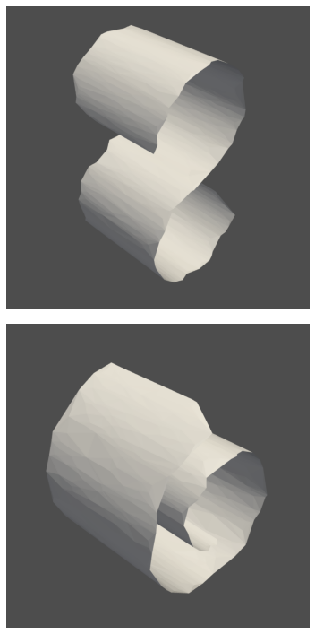
Shapes

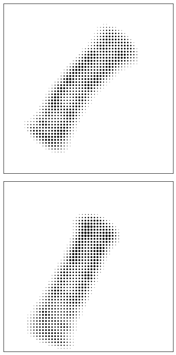
Ours

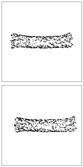
JMDS

(a) S-bended rectangle and Swiss roll (without hole).

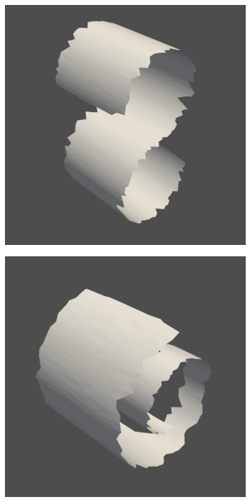
Shapes

Ours

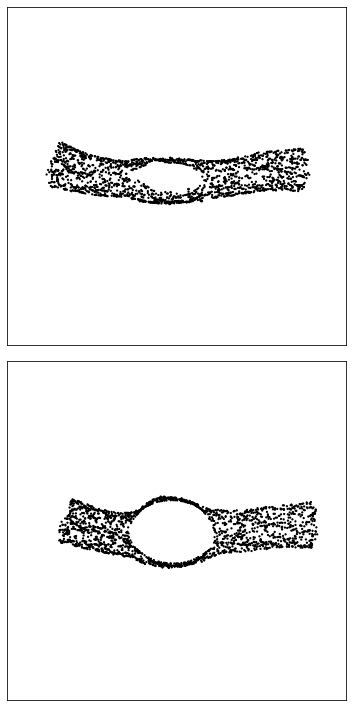
JMDS

(b) S-bended rectangle and Swiss roll with hole.

Figure 8: Embedding and alignment of an S-bended rectangle and a Swiss roll into $\mathbb{R}^{2}$. For our method, we visualize the marginals $P_{Z_{i},\sharp}\alpha$ of the computed 4-plan $\alpha$ in (14) and compare them with JMDS. In the second example (b), JMDS produces an unexpected hole when embedding the S-bended surface.

Human Shapes

Since we are not limited to isometries, we next consider an experiment where isometric embeddings are not possible. More precisely, we embed human shapes from the FAUST dataset Bogo et al. (2014) into $\mathbb{R}^{2}$. For this, we choose $(Z,d_{Z})$ as an equispaced 60$\times$60 grid on $[0,1.3]^{2}\subset\mathbb{R}^{2}$ and apply Algorithm 1 with $\lambda=100$ and $\varepsilon=4\cdot 10^{-4}$. The obtained transport-based embeddings are shown in Figure 11. As comparison, we apply JMDS with $\lambda=10$ and $\varepsilon=4\cdot 10^{-4}$. The 2d representations clearly resemble the 3d human shapes, but JMDS splits some of the extremities.

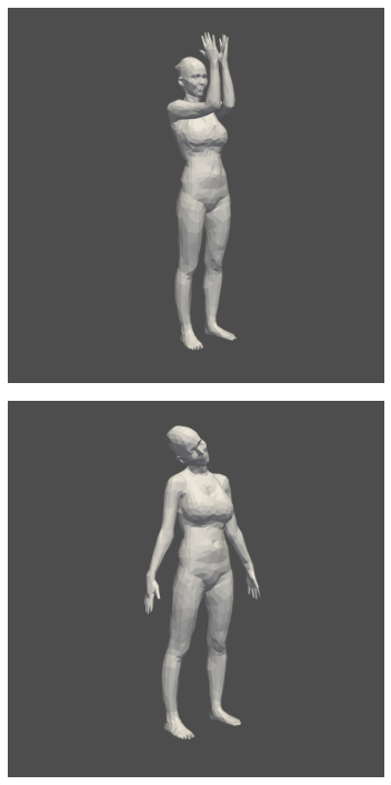
Shapes

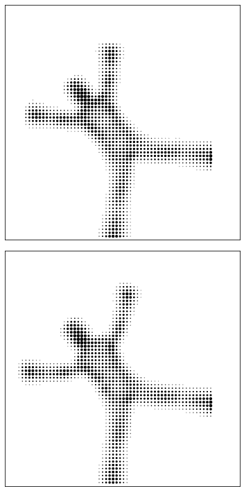
Ours

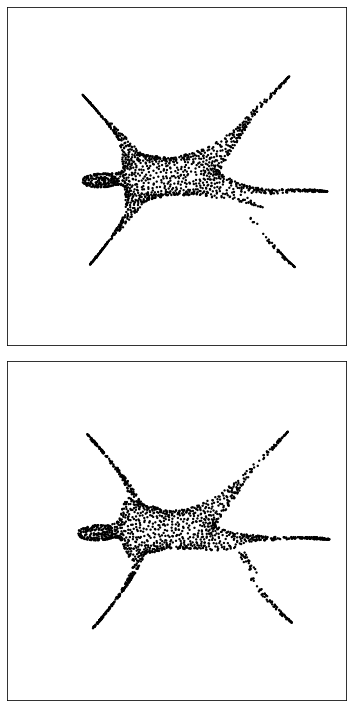
JMDS

(a) Same human shape in different poses.

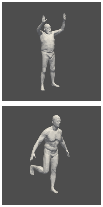
Shapes

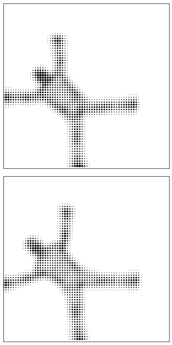
Ours

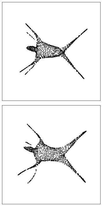
JMDS

(b) Distinct human shapes in different poses.

Figure 11: Embedding and alignment of human shapes from the FAUST dataset into $\mathbb{R}^{2}$. For our method, we visualize the marginals $P_{Z_{i},\sharp}\alpha$ of the computed 4-plan $\alpha$ in (14) and compare them with JMDS. Here JMDS tends to split some of the extremities.

Spherical and Toroidal Embeddings

Finally, we consider the alignment of spherical and toroidal subsets, i.e., the joint embedding into a non-Euclidean space. More precisely, we consider the 3d shapes in the introductory Figure 3. As target space $(Z,d_{Z})$, we choose a 30$\times$30 grid on the canonical parametrization of the sphere $\mathbb{S}(2)$ and the torus $\mathbb{T}(2)=\mathbb{S}(1)\times\mathbb{S}(1)$ equipped with the corresponding geodesic distance. Using $\lambda=10^{3}$ and $\varepsilon=10^{-3}$ for Algorithm 1, we embed the spherical rectangle and a spherical cap, both with a hole, onto the sphere, and the half-torus and toroidal triangle onto the torus. The relaxed embeddings are shown in Figure 3, where the color encodes the mass of the computed marginals. Up to a smoothing due to the incorporated entropic regularization, the transport plans $\gamma_{i}=P_{X_{i}\times Z_{i},\sharp}\alpha$ correspond to the expected isometries.

6.2 Alignment of Feature Spaces

In the next example, we use our method to align different feature spaces occurring in real-world data. More precisely, we consider the genetyping—the determination of the corresponding cell class—of single cells from various measured modalities. Multimodal technologies as proposed in Cheow et al. (2016); Chen et al. (2019) are, however, uncommon such that there is a rising interest in embedding the corresponding features into a joint feature space Demetci et al. (2022); Liu et al. (2019); Chen et al. (2023). Following the experiments of Demetci et al. (2022) for $n$ single cells, our first aim is to assign the recorded features $X_{1}\coloneqq\{x_{1}^{1},\dots,x_{1}^{n}\}\subset\mathbb{R}^{d_{1}}$ from one modality to the features $X_{2}\coloneqq\{x_{2}^{1},\dots,x_{2}^{n}\}\subset\mathbb{R}^{d_{2}}$ of another modality, i.e., to recover the underlying one-to-one correspondence between $x_{1}^{j}$ and $x_{2}^{j}$. Our second goal consists in transferring a classifier from $X_{1}$ to $X_{2}$ in an unsupervised manner.

To achieve both goals, we apply the following methodology:
1. We equip the recorded, uncorrelated features $X_{1}\subset\mathbb{R}^{d_{1}}$ and $X_{2}\subset\mathbb{R}^{d_{2}}$ with specific distances $d_{X_{i}}$ based on the path length in a nearest-ten-neighbor graph, see Cao et al. (2020); Demetci et al. (2022).
2. We equip the constructed metric spaces with the uniform measure to obtain the mm-spaces $\mathbb{X}_{i}\coloneqq(X_{i},d_{X_{i}},\xi_{i})$.
3. Fixing a 20$\times$20 grid $Z\coloneqq\{z^{1},\dots,z^{m}\}\subset\mathbb{R}^{2}$ over $[0,1]^{2}$ equipped with the Euclidean metric, we apply Algorithm 1 with the discretization in Section 5 to compute the 4-plan $\alpha$ in (14).
4. Based on the transport plans $\gamma_{i}\coloneqq P_{X_{i}\times Z_{i},\sharp}\alpha$, we pair $x_{i}^{j}$ with its barycentric projection $\tilde{x}_{i}^{j}\in\mathbb{R}^{m}$ given by

$$\tilde{x}_{i}^{j}\coloneqq\sum_{k=1}^{m}\gamma_{i}^{jk}\,z_{k}\biggm{/}\sum_{k=1}^{m}\gamma_{i}^{jk}.$$ (37)

For the first aim, the identification of the underlying correspondence, we identify $x_{1}^{j}$ with $x_{2}^{k}$ whose barycentric projection $\tilde{x}_{2}^{k}$ is closest to $\tilde{x}_{1}^{j}$. To quantify the quality of the pairing, we rely on the FOSCTTM (fraction of samples closer than the true match) score Liu et al. (2019). More precisely, FOSCTTM is defined by

$$\frac{1}{n^{2}}\,\sum_{j=1}^{n}\#\Bigl{\{}k\in\{1,\dots,n\}:\lVert\tilde{x}_{1}^{j}-\tilde{x}_{2}^{k}\rVert<\lVert\tilde{x}_{1}^{j}-\tilde{x}_{2}^{j}\rVert\Bigr{\}}$$ (38)

and ranges from 0 (perfect identification) to 1.

For the second aim, the transfer of a classifier from $X_{1}$ to $X_{2}$, we exemplarily consider the k-nearest neighbor (KNN) method. More precisely, we use the barycentric projections $\{\tilde{x}_{1}^{1},\dots,\tilde{x}_{1}^{n}\}$ and the corresponding gene type labels of the first modality to classify a feature $x_{2}^{k}$ (more exact $\tilde{x}_{2}^{k}$) from the second modality, where we consider the closest five neighbors. Here, higher classification accuracies (KNN-Acc) indicate better class alignments.

For the experiments, we employ the publicly available datasets from Demetci et al. (2022), where SNAREseq consists of $d_{1}=19$ and $d_{2}=10$ features of $n=1047$ single cells, and scGEM of $d_{1}=34$ and $d_{2}=27$ features of $n=177$ specimens. The computed embedding of $X_{i}$ into $\mathbb{R}^{2}$ of our method and JMDS are visualized in Figure 14. For FOSCTTM and KKN-Acc, we additionally compare both methods with the alignment techniques UnionCom Cao et al. (2020) and SCOT Demetci et al. (2022) using the same distances on $X_{i}$. Note that UnionCom relies on GUMA and t-SNE, whereas SCOT relies on GW and MDS. The results are recorded in Table 1. The hyperparameters of all methods are chosen according to a grid search minimizing the FOSCTTM on a 10% validation split. A further experiment with different feature spaces for MNIST and FashionMNIST is given in Appendix C.

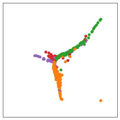
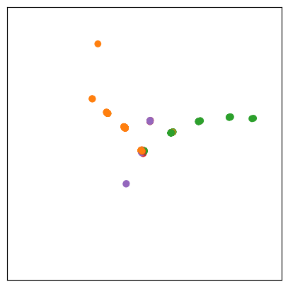
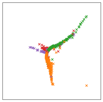
Ours

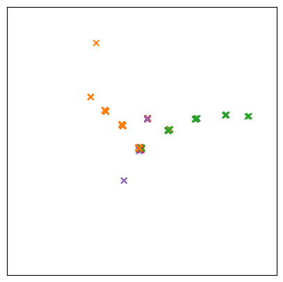
JMDS

(a) SNAREseq dataset

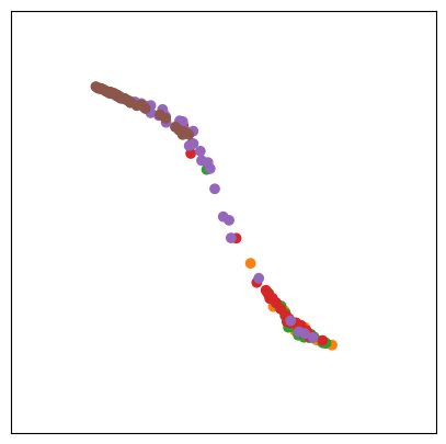
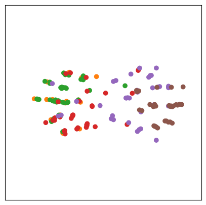
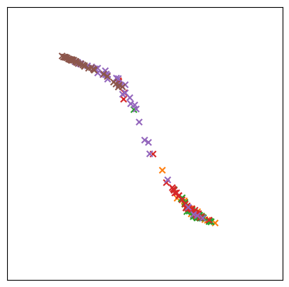
Ours

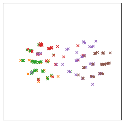
JMDS

(b) scGEM dataset

Figure 14: Joint embedding of two feature spaces into $\mathbb{R}^{2}$ using our method and JMDS. (Top: first feature space, Bottom: second feature space) Both methods align the color-coded classes.

	SNAREseq		scGEM
	FOSCTTM$\downarrow$	KNN-Acc$\uparrow$	FOSCTTM$\downarrow$	KNN-Acc$\uparrow$
${\operatorname{EW}}_{\lambda}$ (Ours)	0.000	0.877	0.000	0.679
JMDS Chen et al. (2023)	0.026	0.896	0.174	0.491
SCOT Demetci et al. (2022)	0.596	0.089	0.248	0.516
UnionCom Cao et al. (2020)	0.257	0.536	0.373	0.270

Table 1: Comparison of the joint embedding of two feature spaces into $\mathbb{R}^{2}$ using our method, JMDS, SCOT, and UnionCom.

6.3 Alignment of Gaussian Mixture Models

In the final example, inspired by Salmona et al. (2024), we want to align Gaussian mixture models (GMMs). For this, we consider the space of 2d Gaussians $\mathcal{N}_{2}=\{\mathcal{N}(\mu,\Sigma)|\mu\in\mathbb{R}^{2},\Sigma\in\mathbb{R}^{2\times 2}\text{ spd.}\}$ equipped with the Wasserstein distance. A GMM can now be interpreted as mm-space $\mathbb{X}=(\mathcal{N}_{2},\operatorname{W},\xi)$ with discrete measure $\xi\coloneqq\sum_{j=1}^{n_{1}}\xi_{j}\,\delta_{\mu_{j},\Sigma_{j}}$. For the experiment, we fit two GMMs to affine-transformed 2d datasets using the expectation-maximization algorithm. Here, we employ the datasets “Blobs” and “Moons” from scikit-learn Pedregosa et al. (2011), see Figure 17. For the alignment of the GMMs, we choose $Z\subset\mathcal{N}_{2}$, where the means form a 15$\times$15 grid over $[0,1]^{2}$ and we use a coarse grid over suitable matrices. Particularly, we consider matrices

$$\Sigma=r^{2}\begin{bmatrix}\sigma_{1}^{2}&\sigma_{12}\\ \sigma_{12}&\sigma_{2}^{2}\end{bmatrix},$$ (39)

where we choose $\sigma_{1}^{2},\sigma_{2}^{2}\in\{0.8,1.\}$ and $\sigma_{12}\in\{-0.2,0.,0.2\}$. The parameter $r^{2}>0$ corresponds to the mean variance of the considered GMMs. Applying Algorithm 1 to compute $\alpha$ in (14), and considering the marginals $\zeta_{i}\coloneqq P_{Z_{i},\sharp}\alpha$, which are again discrete measures on $\mathcal{N}_{2}$, we obtain the aligned GMMs in Figure 17.

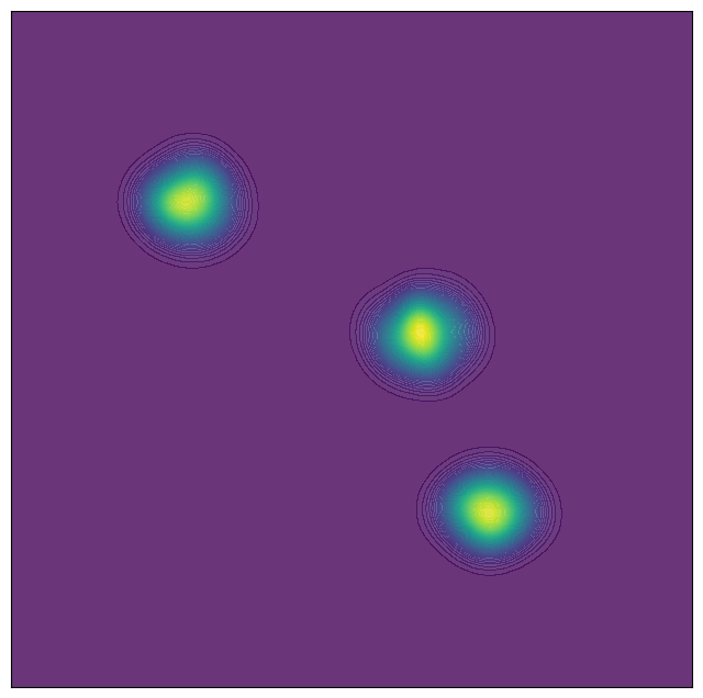
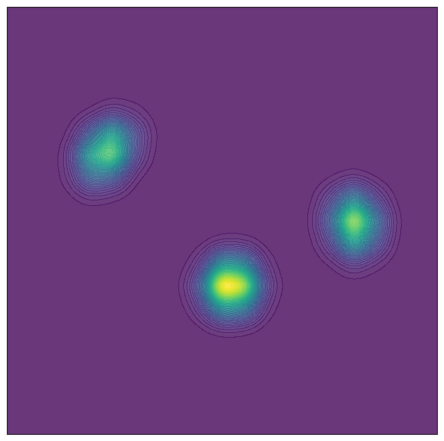
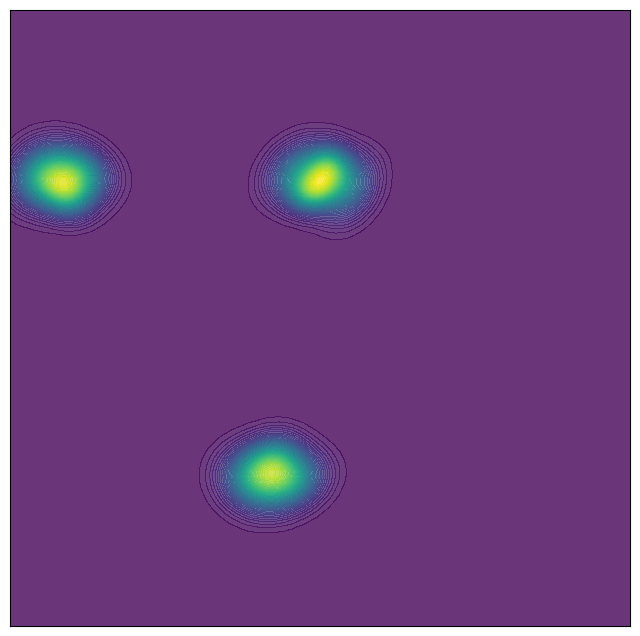
Original

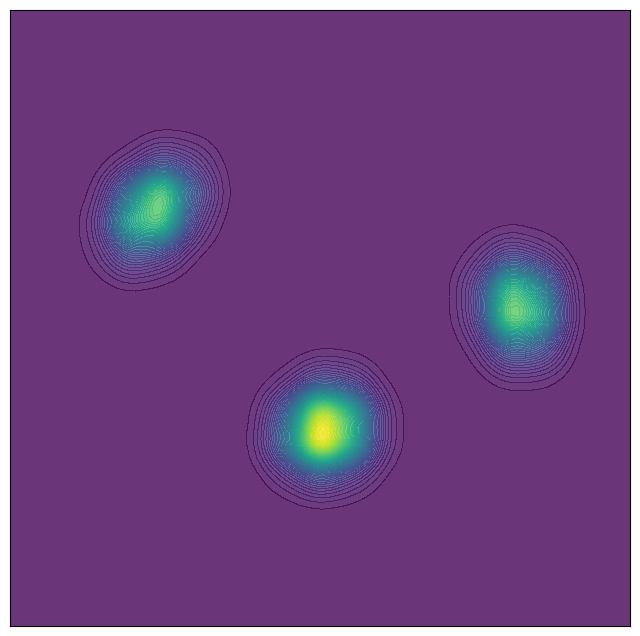
Aligned

(a) Tri-modal GMM

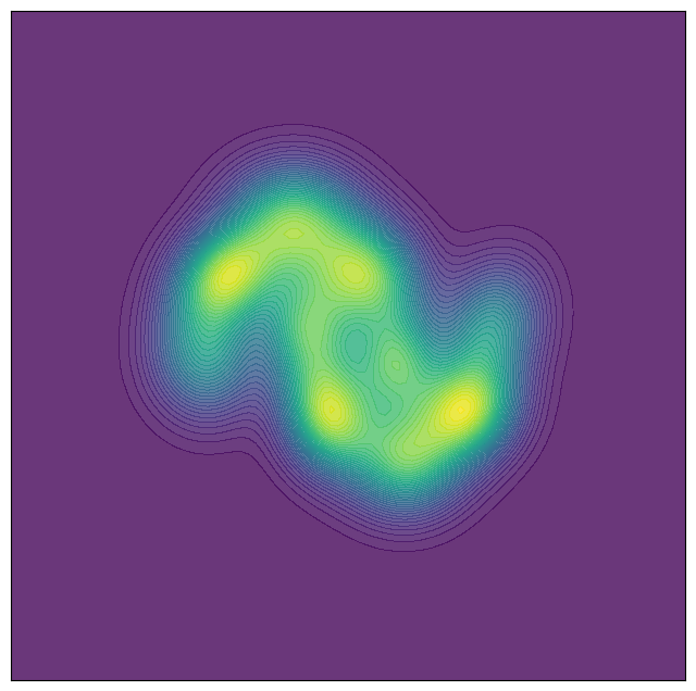
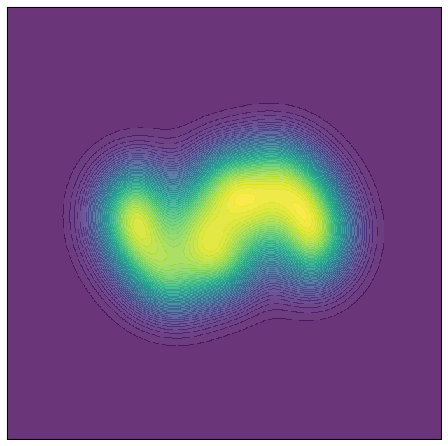
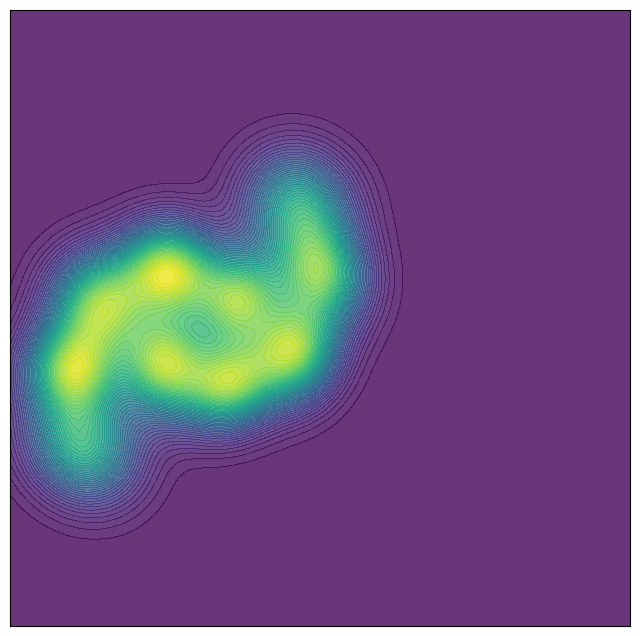
Original

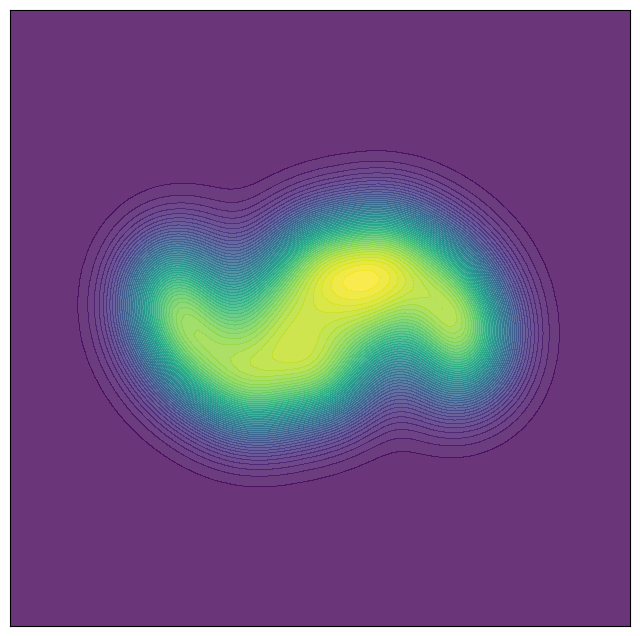
Aligned

(b) “Moons” GMM

Figure 17: Aligenment of GMMs with respect to the Wasserstein distance.

7 Conclusion

We propose an unbalanced OT framework with GW marginal penalization which enables the joint embedding of two datasets based on pairwise intra-dataset distances. While our model can handle the aligned transfer into arbitrary metric spaces, it relies on their appropriate definition. In particular, due to computational restrictions, working on a grid in $\mathbb{R}^{d}$ is restricted to small dimensions $d$. As a future research direction, we are interested in developing a non-Euclidean free-support solver based on existing free-support GW barycenter algorithms Peyré et al. (2016); Vayer et al. (2020a); Beier & Beinert (2024). This may combine our EW_λ approach with a non-Euclidean version of JMDS.

Appendix A Proofs

Proof of Proposition 3.1

The main idea of the proof follows the argumentation for the original embedded Wasserstein distance on Euclidean spaces in Salmona et al. (2024), which we adapt to arbitrary metric spaces. The definiteness follows directly from the definition of the isomorphic equivalence classes, the isometries in EW, and the definiteness of the Wasserstein distance. The symmetry is inherited from the Wasserstein distance too. It remains to show the triangle inequality. Without loss of generality, we take representatives $\mathbb{X}_{i}\coloneqq(Z,d_{Z},\xi_{i})$, $i=1,\dots,3$, such that $\xi_{i}\in\mathcal{P}(Z)$ possess full support. Since the inverse and composition of isometries are isometry, we have

$$\operatorname{EW}(\mathbb{X}_{1},\mathbb{X}_{2})=\inf_{I_{i}:Z\hookrightarrow Z}\operatorname{W}(I_{1,\sharp}\xi_{1},I_{2,\sharp}\xi_{2})=\inf_{I_{i}:Z\hookrightarrow Z}\operatorname{W}(\xi_{1},(I_{1}^{-1}\circ I_{2})_{\sharp}\xi_{2})=\inf_{I:Z\hookrightarrow Z}\operatorname{W}(\xi_{1},I_{\sharp}\xi_{2}).$$

Using the triangle inequality of the Wasserstein distance, we obtain

$$\operatorname{EW}(\mathbb{X}_{1},\mathbb{X}_{2}) =\inf_{I:Z\hookrightarrow Z}\operatorname{W}(\xi_{1},I_{\sharp}\xi_{2})\leq\inf_{I,J:Z\hookrightarrow Z}\operatorname{W}(\xi_{1},J_{\sharp}\xi_{3})+\operatorname{W}(J_{\sharp}\xi_{3},I_{\sharp}\xi_{2})$$

$$=\inf_{J:Z\hookrightarrow Z}\Bigl{(}\operatorname{W}(\xi_{1},J_{\sharp}\xi_{3})+\inf_{I:Z\hookrightarrow Z}\operatorname{W}(J_{\sharp}\xi_{3},I_{\sharp}\xi_{2})\Bigr{)}=\inf_{J:Z\hookrightarrow Z}\Bigl{(}\operatorname{W}(\xi_{1},J_{\sharp}\xi_{3})+\inf_{I:Z\hookrightarrow Z}\operatorname{W}(\xi_{3},(J^{-1}\circ I)_{\sharp}\xi_{2})\Bigr{)}$$

$$=\inf_{J:Z\hookrightarrow Z}\operatorname{W}(\xi_{1},J_{\sharp}\xi_{3})+\inf_{K:Z\hookrightarrow Z}\operatorname{W}(\xi_{3},K_{\sharp}\xi_{2})=\operatorname{EW}(\mathbb{X}_{1},\mathbb{X}_{3})+\operatorname{EW}(\mathbb{X}_{3},\mathbb{X}_{2}). \Box$$

Proof of Proposition 3.2. Let $X\in\{X_{i}:i=1,2\}$. We equip the space of continuous functions $C(X,Z)$ with the topology of uniform convergence $d(f,g)\coloneqq\max_{x\in X}d_{Z}(f(x),g(x))$.

1. First, we we show that

$$\operatorname{Iso}(X,Z)\coloneqq\{I:X\hookrightarrow Z\}\subset C(X,Z)$$

is compact. Since $(Z,d_{Z})$ is compact, we see immediately that $\operatorname{Iso}(X,Z)$ is pointwise bounded. Moreover, since all functions in $\operatorname{Iso}(X,Z)$ are isometries the set is equicontinuous. By the Theorem of Arzelà–Ascoli Munkres (2000) (Thm. 47.1), this gives the relative compactness of $\operatorname{Iso}$. Further, $\operatorname{Iso}(X,Z)\subset C(X,Z)$ is closed and thus compact, since we have for any sequence of isometies $(I_{n})_{n}$ from $X$ to $Z$ converging to some $I\in C(X,Z)$ that

$$d_{X}(x,x^{\prime})=d_{Z}(I_{n}(x),I_{n}(x^{\prime}))\rightarrow d_{Z}(I(x),I(x^{\prime}))$$

as $n\to\infty$, so that $I\in\operatorname{Iso}(X,Z)$. Then also $\operatorname{Iso}(X_{1},Z)\times\operatorname{Iso}(X_{2},Z)$ is compact.
2. Next, we show that the functional

$$F(I_{1},I_{2})\coloneqq\operatorname{W}(I_{1,\sharp}\xi_{1},I_{2,\sharp}\xi_{2})$$

in (6) is lower semi-continuous on $\operatorname{Iso}(X_{1},Z)\times\operatorname{Iso}(X_{2},Z)$. For $i=1,2$, let $(I_{i,n})_{n\in\mathbb{N}}\subset\operatorname{Iso}(X_{i},Z)$ and $I_{i}\in\operatorname{Iso}(X_{1},Z)$ with $I_{i,n}\to I_{i}$ as $n\to\infty$. Then, for all $\varphi\in C(Z,\mathbb{R})$, it holds by the dominated convergence theorem that

$$\int_{Z}\varphi\,\mathrm{d}(I_{i,n})_{\sharp}\xi_{i}=\int_{X}\varphi\circ I_{i,n}\,\mathrm{d}\xi_{i}$$ (40)

$$\rightarrow\int_{X_{i}}\varphi\circ I_{i}\,\mathrm{d}\xi_{i}=\int_{Z}\varphi\,\mathrm{d}I_{i,\sharp}\xi_{i}\;\text{ as }\;n\to\infty.$$ (41)

Thus we obtain the weak convergence $(I_{i,n})_{\sharp}\xi_{i}\rightharpoonup I_{i,\sharp}\xi_{i}$. Finally, due to the joint weak lower semi-continuity of the Wasserstein distance Ambrosio et al. (2005) (Lemma. 7.1.4), we get the desired lower semi-continuity of $F$.

Finally, application of the Weierstrass theorem yields the assertion. $\Box$

Proof of Proposition 3.3. Since $\mathcal{P}(Z\times Z)$ is weakly compact, the existence of a minimizer follows by Weierstrass’ theorem, see, e.g., Mordukhovich & Nam (2022) (Thm. 2.164), once we can show that the objective function

$$F(\pi) \coloneqq\int_{Z\times Z}d_{Z}^{2}(z,z^{\prime})\,\mathrm{d}\pi(z,z^{\prime})+\lambda\sum_{i=1}^{2}\operatorname{GW}^{2}(\mathbb{X}_{i},(Z,d_{Z},P_{i,\sharp}\pi))$$ (42)

in (8) is weakly lower semi-continuous.

Let $(\pi_{n})_{n\in\mathbb{N}}\subset\mathcal{P}(Z\times Z)$ and $\pi\in\mathcal{P}(Z\times Z)$ be such that $\pi_{n}\rightharpoonup\pi$ as $n\to\infty$. We handle the terms of $F$ separately. Since $d_{Z}^{2}$ is continuous in both arguments, we obtain by definition of the weak convergence that

$$\int_{Z\times Z}d_{Z}^{2}(z,z^{\prime})\,\mathrm{d}\pi_{n}(z,z^{\prime})\rightarrow\int_{Z\times Z}d_{Z}^{2}(z,z^{\prime})\,\mathrm{d}\pi(z,z^{\prime})$$

as $n\to\infty$. We turn to the GW terms. For $i=1,2$, set

$$\mu_{i,n}\coloneqq P_{i,\sharp}\pi_{n}\quad\text{and}\quad\mu_{i}\coloneqq P_{i,\sharp}\pi.$$

Then the weak lower semi-continuity of the marginal projection operators yields $\mu_{i,n}\rightharpoonup\mu_{i}$ as $n\to\infty$. Now let $\gamma_{i,n}\in\Pi(\xi_{i},\mu_{i,n})$ be a solution of $\operatorname{GW}(\mathbb{X}_{i},(Z,d_{Z},\mu_{i,n}))$, $n\in\mathbb{N}$. As $(\gamma_{i,n})_{n\in\mathbb{N}}\subset\mathcal{P}(X_{i}\times Z)$ and the latter is weakly compact, we can choose a converging subsequence again denoted by $(\gamma{i,n})_{n\in\mathbb{N}}$, such that $\gamma_{i,n}\rightharpoonup\gamma_{i}\in\mathcal{P}(X_{i}\times Z)$. Using again the weak continuity of the marginal projection, we get $\gamma\in\Pi(\xi_{i},\mu_{i})$. Therefore, it holds

$$\operatorname{GW}^{2}(\mathbb{X}_{i},(Z,d_{Z},P_{i,\sharp}\pi))=\operatorname{GW}^{2}(\mathbb{X}_{i},(Z,d_{Z},\mu_{i}))\leq\iint\limits_{(X_{i}\times Z)^{2}}(d_{X_{i}}(x_{i},x_{i}^{\prime})-d_{Z}(z,z^{\prime}))^{2}\,\mathrm{d}\gamma(x_{i},z)\,\mathrm{d}\gamma(x_{i}^{\prime},z^{\prime})$$

and by continuity of the integrand and the fact that $(\gamma_{i,n}\otimes\gamma_{i,n})\rightharpoonup(\gamma_{i}\otimes\gamma_{i})$, see, e.g., Bogachev (2018) (Prop. 2.7.8) further

$$\operatorname{GW}^{2}(\mathbb{X}_{i},(Z,d_{Z},P_{i,\sharp}\pi)) \leq\lim_{n\to\infty}\!\iint_{(X_{i}\times Z)^{2}}(d_{X_{i}}(x_{i},x_{i}^{\prime})-d_{Z}(z,z^{\prime}))^{2}\,\mathrm{d}\gamma_{i,n}(x_{i},z)\,\mathrm{d}\gamma_{i,n}(x_{i}^{\prime},z^{\prime})$$

$$=\lim_{n\to\infty}\operatorname{GW}^{2}(\mathbb{X}_{i},(Z,d_{Z},\mu_{i,n}))=\lim_{n\to\infty}\operatorname{GW}^{2}(\mathbb{X}_{i},(Z,d_{Z},P_{i,\sharp}\pi_{n})).$$

This gives lower semi-continuity of the functional of $F$. $\Box$

Proof of Proposition 3.4. 1. First, we show that

$$\operatorname{EW}_{\lambda}(\mathbb{X}_{1},\mathbb{X}_{2})\leq\operatorname{EW}(\mathbb{X}_{1},\mathbb{X}_{2}),\qquad\lambda>0.$$ (43)

To this end, let $I_{i}:X_{i}\hookrightarrow Z_{i}$ be isometries realizing $\operatorname{EW}(\mathbb{X}_{1},\mathbb{X}_{2})$, i.e.,

$$\operatorname{EW}(\mathbb{X}_{1},\mathbb{X}_{2})=\operatorname{W}(I_{1,\sharp}\xi_{1},I_{2,\sharp}\xi_{2}).$$

By definition of the GW distance, we have $\operatorname{GW}(\mathbb{X}_{i},(Z_{i},d_{Z_{i}},I_{i,\sharp}\xi_{i})=0$, $i=1,2$. Then we obtain for $\tilde{\pi}\in\Pi_{0}(I_{1,\sharp}\xi_{1},I_{2,\sharp}\xi_{2})$ that

$$\operatorname{EW}_{\lambda}(\mathbb{X}_{1},\mathbb{X}_{2}) \leq\Big{(}\int_{Z_{1}\times Z_{2}}d_{Z}^{2}(z,z^{\prime})\,\mathrm{d}\tilde{\pi}(z,z^{\prime})\Big{)}^{\frac{1}{2}}=\operatorname{W}(I_{1,\sharp}\xi_{1},I_{2,\sharp}\xi_{2})=\operatorname{EW}_{(Z,d_{Z})}(\mathbb{X}_{1},\mathbb{X}_{2}).$$

2. Now let $(\lambda_{n})_{n\in\mathbb{N}}$ with $\lambda_{n}\to\infty$ as $n\to\infty$, and let $\pi_{n}\in\mathcal{P}(Z\times Z)$ realize $\operatorname{EW}_{\lambda_{n}}(\mathbb{X}_{1},\mathbb{X}_{2})$. Then we conclude by (43) that

$$\operatorname{EW}(\mathbb{X}_{1},\mathbb{X}_{2})\geq\operatorname{EW}_{\lambda_{n}}(\mathbb{X}_{1},\mathbb{X}_{2}) =\int_{Z\times Z}d_{Z}(z,z^{\prime})\,\mathrm{d}\pi_{n}(z,z^{\prime})+\lambda_{n}\sum_{i=1}^{2}\operatorname{GW}(\mathbb{X}_{i},(Z,d_{Z},P_{i,\sharp}\pi_{n}))$$

$$\geq\lambda_{n}\sum_{i=1}^{2}\operatorname{GW}(\mathbb{X}_{i},(Z,d_{Z},(P_{i})_{\#}\pi_{n})).$$

Hence, we obtain for $i=1,2$ that

$$\operatorname{GW}(\mathbb{X}_{i},(Z,d_{Z},(P_{i})_{\#}\pi_{n}))\to 0\;\text{ as }\;n\to\infty.$$

Since $(\pi_{n})_{n\in\mathbb{N}}$ is contained in the weakly compact set $\mathcal{P}(Z\times Z)$, there exists a subsequence (denoted in the same way) which weakly converges to some $\pi\in\mathcal{P}(Z\times Z)$. Then also $P_{i,\sharp}\pi_{n}$ converges weakly to $P_{i,\sharp}\pi$, $i=1,2$ and we obtain as in the proof of (3.3), that

$$\operatorname{GW}(\mathbb{X}_{i},(Z,d_{Z},P_{i,\sharp}\pi))\leq\lim_{n\to\infty}\operatorname{GW}(\mathbb{X}_{i},(Z,d_{Z},P_{i,\sharp}\pi_{n}))=0.$$

Thus, there exist isometries $I_{i}:X_{i}\hookrightarrow Z$ with $P_{i,\sharp}\pi=I_{i,\sharp}\xi_{i}$, $i=1,2$, i.e., $\pi\in\Pi(I_{1,\sharp}\xi_{1},I_{2,\sharp}\xi_{2})$. Finally, we obtain for any fixed $\lambda>0$ that

$$\operatorname{EW}(\mathbb{X}_{1},\mathbb{X}_{2}) \leq\Big{(}\int_{Z_{1}\times Z_{2}}d_{Z}^{2}(z_{1},z_{2})\,\mathrm{d}\pi(z_{1},z_{2})\Big{)}^{\frac{1}{2}}$$

$$=\Big{(}\int_{Z_{1}\times Z_{2}}d_{Z}^{2}(z_{1},z_{2})\,\mathrm{d}\pi(z_{1},z_{2})+\lambda\sum_{i=1}^{2}\underbrace{\operatorname{GW}(\mathbb{X}_{i},(Z,d_{Z},P_{i,\sharp}\pi))}_{=0}\Big{)}^{\frac{1}{2}}$$

$$\leq\lim_{n\to\infty}\Big{(}\int_{Z_{1}\times Z_{2}}d_{Z}^{2}(z_{1},z_{2})\,\mathrm{d}\pi_{n}(z_{1},z_{2})+\lambda\sum_{i=1}^{2}\operatorname{GW}(\mathbb{X}_{i},(Z,d_{Z},P_{i,\sharp}\pi_{n}))\Big{)}^{\frac{1}{2}}$$

$$\leq\lim_{n\to\infty}\operatorname{EW}_{\lambda_{n}}(\mathbb{X}_{1},\mathbb{X}_{2})\leq\operatorname{EW}(\mathbb{X}_{1},\mathbb{X}_{2}).$$

Hence $\pi\in\Pi(I_{1,\sharp}\xi_{1},I_{2,\sharp}\xi_{2})$ and

$$\operatorname{EW}(\mathbb{X}_{1},\mathbb{X}_{2}) =\inf_{\begin{subarray}{c}J_{i}:X_{i}\hookrightarrow Z,i=1,2\end{subarray}}\operatorname{W}(J_{1,\sharp}\xi_{1},J_{2,\sharp}\xi_{2})=\Big{(}\int_{Z_{1}\times Z_{2}}d_{Z}^{2}(z_{1},z_{2})\,\mathrm{d}\pi(z_{1},z_{2})\Big{)}^{\frac{1}{2}}$$ (44)

implies that $(I_{1},I_{2})$ minimizes $\operatorname{EW}(\mathbb{X}_{1},\mathbb{X}_{2})$ and $\pi$ realizes $\operatorname{W}(I_{1,\sharp}\xi_{1},I_{2,\sharp}\xi_{2})$. $\Box$

Appendix B Numerical Studies on GW, EW, and EW_λ

Our approach enables geometrically meaningful data comparison as we can approximate the EW metric on general metric spaces $Z$. We validate this in two experiments.

Approximation of $\operatorname{EW}$ by $\operatorname{EW}_{\lambda}$ for Synthetic Circular Data

Consider circular mm-spaces $\mathbb{X}_{i}=(\mathbb{S}^{1},d_{\mathbb{S}^{1}},\xi_{i})$ with $(Z,d_{Z})=(\mathbb{S}^{1},d_{\mathbb{S}^{1}})$, where ($\mathbb{S}^{1}$, $d_{\mathbb{S}^{1}}$) denotes the circle equipped with a circular distance. We set $\xi_{1}$ uniformly distributed and $\xi_{2}$ according to the density of a von Mises distribution with increasing dispersion parameter $\kappa$. Note that the von Mises distribution takes the form of a uniform distribution for $\kappa=0$ and becomes more concentrated for $\kappa\to\infty$. Due to the rotational invariance of the uniform distribution on the circle, the embedded Wasserstein distance can easily be calculated in this case as it coincides with the Wasserstein distance. Thus, we can ignore the isometry in $\operatorname{EW}$ and directly calculate $\operatorname{EW}$ by solving the linear program underlying the OT problem. We discretize the circle into 360 bins and estimate $\operatorname{EW}_{\lambda}$ for different choices of $\kappa$ and $\lambda$. The results in Figure 19 show an improved approximation of $\operatorname{EW}$ for larger $\lambda$ as announced in Proposition 3.4. Indeed, we have an excellent fit for $\lambda=20$, whereas $\lambda=0.2$ leads to an underestimation.

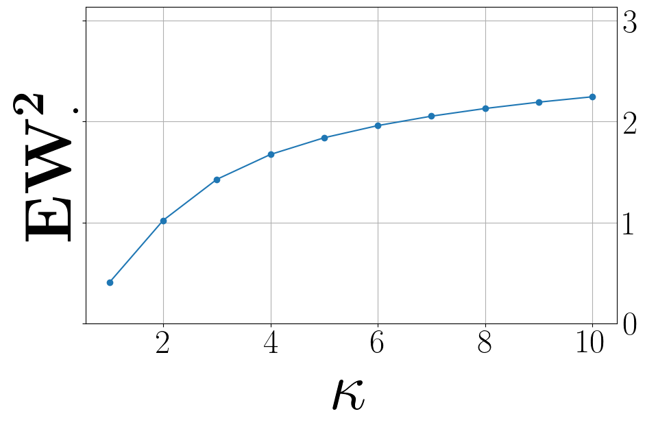
$\operatorname{EW}^{2}$ ($\lambda=\infty$)

$\operatorname{EW}^{2}_{\lambda}$ ($\lambda=20$)

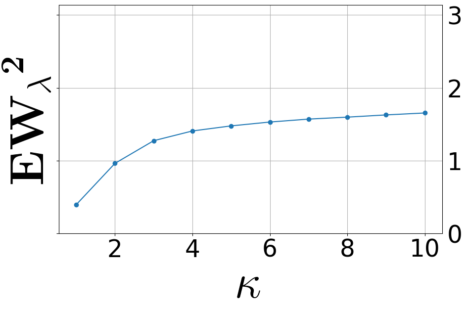
$\operatorname{EW}^{2}_{\lambda}$ ($\lambda=0.2$)

Figure 19: Comparison of $\operatorname{EW}$ with $\operatorname{EW}_{\lambda}$ for different $\lambda$. While the curves for $\operatorname{EW}$ (left) and $\operatorname{EW}_{20}$ (middle) are almost identical, those for $\operatorname{EW}_{0.2}$ (right) is consistently smaller.

2d Shape Matching

Next, we compare randomly rotated gray-value images. We can describe such images as mm-spaces $\mathbb{X}_{i}=(X,d,\xi_{i})$ where $X\subset\mathbb{R}^{2}$ is a grid that describes the pixel positions equipped with the Euclidean metric and $\xi_{i}$ is the pixel intensity, see Beier et al. (2023). We use $(Z,d_{Z})=(X,d)$. We apply random affine transformations, i.e., translations and rotations, to the first 10 FashionMNIST Xiao et al. (2017) training images from the classes “Trouser”, “Pullover” and “Sneaker”, respectively. Then we compute $\operatorname{W}$, $\operatorname{GW}$ and $\operatorname{EW}_{\lambda}$ for $\lambda=20$. The results are displayed in Figure 21. As expected, the Wasserstein distance cannot recover the class structure due to the affine transformations, whereas $\operatorname{EW}_{\lambda}$ and GW capture the class structure. Moreover, we see that the distance matrices of $\operatorname{EW}_{\lambda}$ and GW display almost identical patterns, up to scaling.

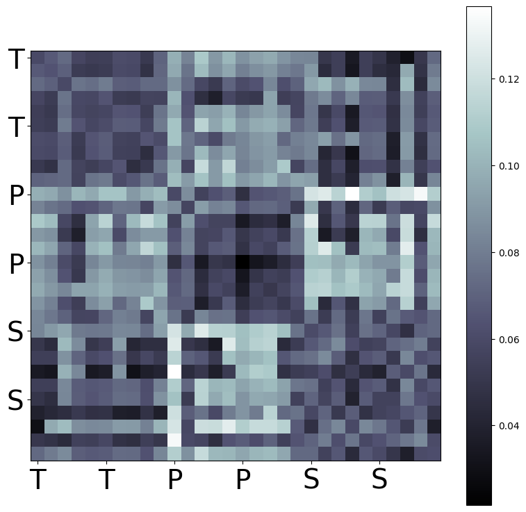
$\operatorname{EW}_{\lambda}$ ($\lambda=20$)

$\operatorname{GW}$

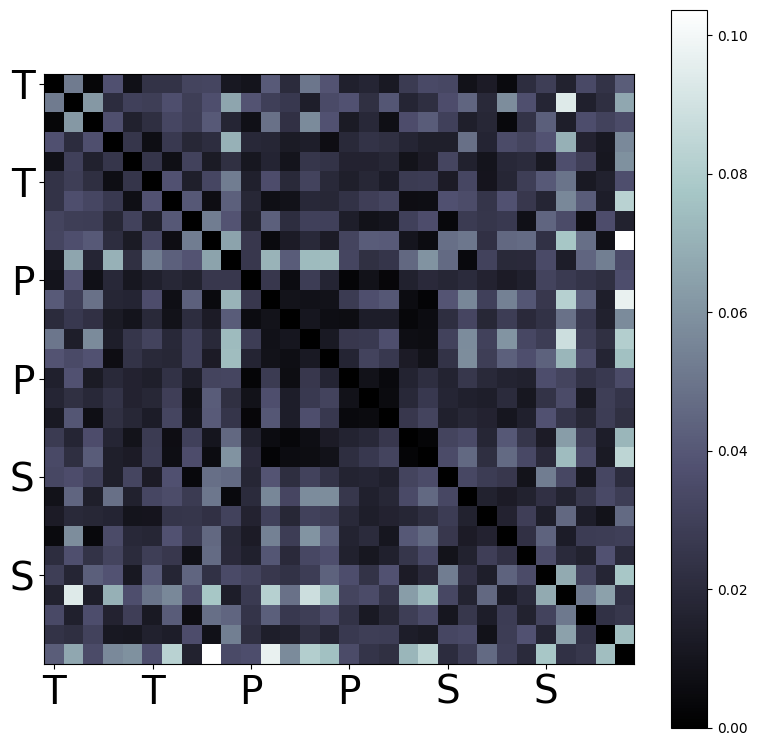
$\operatorname{W}$

Figure 21: Pairwise $\operatorname{W}$, $\operatorname{GW}$ and $\operatorname{EW}_{20}$ distances of 10 randomly rotated and translated images from each of the “Trouser” (T), “Pullover” (P), and “Sneaker” (S) FashionMNIST classes. Smaller distances are darker. The class block structure is recovered with $\operatorname{EW}_{\lambda}$ and $\operatorname{GW}$, but not with Wasserstein.

Appendix C Further Example for Comparing Feature Spaces

As an addition to the genetyping experiment, we present another experiment with real-world data based on latent spaces. We consider the task of comparing the 4d latent spaces of an auto-encoder (AE) versus a variational auto-encoder (VAE), trained on FashionMNIST Xiao et al. (2017). For this purpose, we train a simple convolutional AE with two convolutional layers and one linear layer for the encoder and the decoder. We train the AE with the MSE loss and the VAE with the log-likelihood loss for 10 epochs on the canonical training data splits. Subsequently, we embed the test data using the resulting AE and VAE into the 4d latent spaces. Note that such distinct AE trained on the same dataset generally produce incomparable embeddings. For our experiment, we consider the first 100 data points of the test split. We choose $Z$ as an equispaced 20$\times$20 grid on $[0,1.3]\subset\mathbb{R}^{2}$ with the Euclidean distance. We follow the same evaluation routine as in Subsection 6.2 for parameter selection and visualization. The joint embeddings are visualized in Figure 24. Comparing FOSCTTM and KNN, we see again a good embedding quality for our approach, see the figure caption.

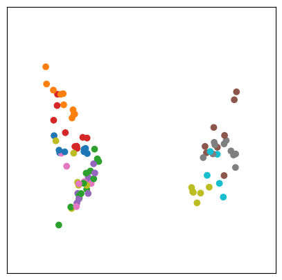
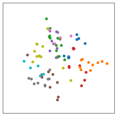
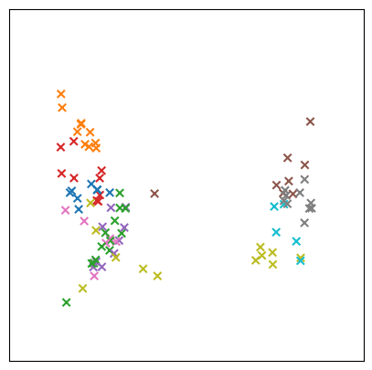
Ours

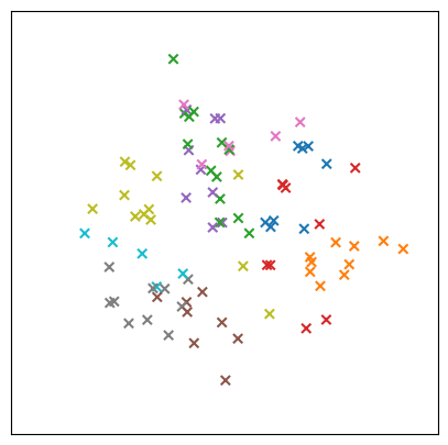
JMDS

Figure 24: Joint embedding of the FashionMNIST latent space of an AE and a VAE into $\mathbb{R}^{2}$ using our method and JMDS. The AE latent space is on the top and the VAE latent space is on the bottom. Both methods align the color-coded classes. A quantitative comparison shows that our model achieves a better FOSCTTM (0.040) than JMDS (0.042), whereas our KNN-Accuracy (0.589) is slightly worse than the one of JMDS (0.644).

References

- Alaya et al. (2022) Alaya, M. Z., Bérar, M., Gasso, G., and Rakotomamonjy, A. Theoretical guarantees for bridging metric measure embedding and optimal transport. Neurocomputing, 468:416–430, 2022.
- Alvarez-Melis et al. (2019) Alvarez-Melis, D., Jegelka, S., and Jaakkola, T. S. Towards optimal transport with global invariances. In International Conference on Artificial Intelligence and Statistics (AISTATS), volume 89 of Proceedings of Machine Learning Research, pp. 1870–1879. PMLR, 2019.
- Ambrosio et al. (2005) Ambrosio, L., Gigli, N., and Savaré, G. Gradient Flows in Metric Spaces and in the Space of Probability Measures. Birkhäuser, Basel, 2005. ISBN 978-3-7643-2428-5; 3-7643-2428-7.
- Amodio & Krishnaswamy (2018) Amodio, M. and Krishnaswamy, S. MAGAN: Aligning biological manifolds. In International Conference on Machine Learning (ICML), pp. 215–223. PMLR, 2018.
- Beier & Beinert (2024) Beier, F. and Beinert, R. Tangential fixpoint iterations for Gromov–Wasserstein barycenters. arXiv preprint arXiv:2403.08612, 2024.
- Beier et al. (2022) Beier, F., von Lindheim, J., Neumayer, S., and Steidl, G. Unbalanced multi-marginal optimal transport. J. Math. Imaging Vision, 65:394–413, 2022.
- Beier et al. (2023) Beier, F., Beinert, R., and Steidl, G. Multi-marginal Gromov–Wasserstein transport and barycentres. Inf. Inference, 12(4):2753–2781, 10 2023. ISSN 2049-8772.
- Bogachev (2018) Bogachev, V. I. Weak convergence of measures. Number 234 in Mathematical Surveys and Monographs. American Mathematical Society, Providence, RI, 2018.
- Bogo et al. (2014) Bogo, F., Romero, J., Loper, M., and Black, M. J. FAUST: Dataset and evaluation for 3D mesh registration. In IEEE Conference on Computer Vision and Pattern Recognition (CVPR). IEEE, June 2014.
- Cao et al. (2020) Cao, K., Bai, X., Hong, Y., and Wan, L. Unsupervised topological alignment for single-cell multi-omics integration. Bioinformatics, 36(1):i48–i56, 2020.
- Cao et al. (2022) Cao, K., Hong, Y., and Wan, L. Manifold alignment for heterogeneous single-cell multi-omics data integration using Pamona. Bioinformatics, 38(1):211–219, 2022.
- Carroll & Arabie (1998) Carroll, J. D. and Arabie, P. Multidimensional scaling. In Birnbaum, M. H. (ed.), Measurement, Judgment and Decision Making, pp. 179–250. Elsevier, 1998.
- Chen et al. (2023) Chen, D., Fan, B., Oliver, C., and Borgwardt, K. Unsupervised manifold alignment with joint multidimensional scaling. In International Conference on Learning Representations (ICLR). OpenReview, 2023.
- Chen et al. (2019) Chen, S., Lake, B. B., and Zhang, K. High-throughput sequencing of the transcriptome and chromatin accessibility in the same cell. Nat. Biotechnol., 37:1452–1457, 2019.
- Cheow et al. (2016) Cheow, L. F., Courtois, E. T., Tan, Y., Viswanathan, R., Xing, Q., Tan, R. Z., Tan, D. S. W., Robson, P., Loh, Y.-H., Quake, S. R., and Burkholder, W. F. Single-cell multimodal profiling reveals cellular epigenetic heterogeneity. Nat. Methods, 13:833–836, 2016.
- Cui et al. (2014) Cui, Z., Chang, H., Shan, S., and Chen, X. Generalized unsupervised manifold alignment. In Advances in Neural Information Processing Systems (NeurIPS), volume 27. Curran Associates, Inc., 2014.
- Cuturi & Avis (2014) Cuturi, M. and Avis, D. Ground metric learning. JMLR, 15(1):533–564, 2014.
- Demetci et al. (2022) Demetci, P., Santorella, R., Sandstede, B., Noble, W. S., and Singh, R. SCOT: single-cell multi-omics alignment with optimal transport. J. Comput. Biol., 29(1):3–18, 2022.
- Deng et al. (2024) Deng, C., Gao, J., Lu, K., Luo, F., Sun, H., and Xin, C. Neuc-MDS: Non-Euclidean multidimensional scaling through bilinear forms. In Advances on Neural Information Processing Systems (NeurIPS), volume 38. Curran Associates, Inc., 2024.
- Dijkstra (1959) Dijkstra, E. W. A note on two problems in connexion with graphs. Numer. Math., 1:269–271, 1959.
- Grave et al. (2019) Grave, E., Joulin, A., and Berthet, Q. Unsupervised alignment of embeddings with Wasserstein procrustes. In Chaudhuri, K. and Sugiyama, M. (eds.), International Conference on Artificial Intelligence and Statistics (AISTATS), volume 89 of Proceedings of Machine Learning Research, pp. 1880–1890. PMLR, 2019.
- Greenacre et al. (2022) Greenacre, M., Groenen, P. J., Hastie, T., d’Enza, A. I., Markos, A., and Tuzhilina, E. Principal component analysis. Nat. Rev. Methods Primers, 2(1):100, 2022.
- Heitz et al. (2021) Heitz, M., Bonneel, N., Coeurjolly, D., Cuturi, M., and Peyré, G. Ground metric learning on graphs. J. Math. Imaging Vision, 63:89–107, 2021.
- Kingma et al. (2019) Kingma, D. P., Welling, M., et al. An introduction to variational autoencoders. Found. Trends Theor. Comput. Sci., 12(4):307–392, 2019.
- Liu et al. (2019) Liu, J., Huang, Y., Singh, R., Vert, J.-P., and Noble, W. S. Jointly embedding multiple single-cell omics measurements. In 19th International Workshop on Algorithms in Bioinformatics (WABI 2019), volume 143 of Leibniz International Proceedings in Informatics (LIPIcs), pp. 10:1–10:13, 2019.
- McInnes et al. (2018) McInnes, L., Healy, J., Saul, N., and Großberger, L. UMAP: Uniform manifold approximation and projection. J. Open Source Softw., 3(29), 2018.
- Mémoli (2011) Mémoli, F. Gromov–Wasserstein distances and the metric approach to object matching. Found. Comput. Math., 11(4):417–487, 2011.
- Mordukhovich & Nam (2022) Mordukhovich, B. S. and Nam, N. M. Convex analysis and beyond. Springer, 2022.
- Munkres (2000) Munkres, J. Topology. Featured Titles for Topology. Prentice Hall, Incorporated, 2000.
- Paty & Cuturi (2019) Paty, F.-P. and Cuturi, M. Subspace robust Wasserstein distances. In International Conference on Machine Learning (ICML), pp. 5072–5081. PMLR, 2019.
- Pedregosa et al. (2011) Pedregosa, F., Varoquaux, G., Gramfort, A., Michel, V., Thirion, B., Grisel, O., Blondel, M., Prettenhofer, P., Weiss, R., Dubourg, V., et al. Scikit-learn: Machine learning in Python. JMLR, 12:2825–2830, 2011.
- Peyré et al. (2016) Peyré, G., Cuturi, M., and Solomon, J. Gromov–Wasserstein averaging of kernel and distance matrices. In Balcan, M. F. and Weinberger, K. Q. (eds.), International Conference on Machine Learning (ICML), volume 48 of Proceedings of Machine Learning Research, pp. 2664–2672. PMLR, 2016.
- Roweis & Saul (2000) Roweis, S. T. and Saul, L. K. Nonlinear dimensionality reduction by locally linear embedding. Science, 290(5500):2323–2326, 2000.
- Salmona et al. (2024) Salmona, A., Desolneux, A., and Delon, J. Gromov–Wasserstein-like distances in the Gaussian mixture models space. TMLR, 2024.
- Sturm (2006) Sturm, K.-T. On the geometry of metric measure spaces. Acta Mathematica, 196(1):65 – 131, 2006.
- Sturm (2023) Sturm, K.-T. The space of spaces: curvature bounds and gradient flows on the space of metric measure spaces, volume 290 of Memoirs of the American Mathematical Society. American Mathematical Society, Providence, 2023.
- Séjourné et al. (2021) Séjourné, T., Vialard, F.-X., and Peyré, G. The unbalanced Gromov–Wasserstein distance: Conic formulation and relaxation. In Ranzato, M., Beygelzimer, A., Dauphin, Y., Liang, P., and Vaughan, J. W. (eds.), Advances in Neural Information Processing Systems (NeurIPS), volume 34 of Advances in Neural Information Processing Systems. Curran Associates, Inc., 2021.
- Van der Maaten & Hinton (2008) Van der Maaten, L. and Hinton, G. Visualizing data using t-SNE. JMLR, 9(86):2579–2605, 2008.
- Vayer et al. (2020a) Vayer, T., Chapel, L., Flamary, R., Tavenard, R., and Courty, N. Fused Gromov–Wasserstein distance for structured objects. Algorithms, 13(9):212, 2020a.
- Vayer et al. (2020b) Vayer, T., Redko, I., Flamary, R., and Courty, N. Co-optimal transport. In Larochelle, H., Ranzato, M., Hadsell, R., Balcan, M., and Lin, H. (eds.), Advances in Neural Information Processing Systems (NeurIPS), volume 33 of Advances in Neural Information Processing Systems, pp. 17559–17570. Curran Associates, Inc., 2020b.
- Xiao et al. (2017) Xiao, H., Rasul, K., and Vollgraf, R. Fashion-MNIST: A novel image dataset for benchmarking machine learning algorithms. arXiv preprint arXiv:1708.07747, 2017.