Physics-Informed Recurrent Network for Gas Pipeline Network Parameters Identification

Abstract

As a part of the integrated energy system (IES), gas pipeline networks can provide additional flexibility to power systems through coordinated optimal dispatch. An accurate pipeline network model is critical for the optimal operation and control of IESs. However, inaccuracies or unavailability of accurate pipeline parameters often introduce errors in the mathematical models of such networks. This paper proposes a physics-informed recurrent network (PIRN) model to identify the state-space model of gas pipelines. The approach combines data-driven learning from measurement data with the fluid dynamics described by partial differential equations. By embedding the physical state-space model within the recurrent network, parameter identification is transformed into a training process for a PIRN. Similar to standard recurrent neural networks, this model can be implemented using the PyTorch framework and trained via backpropagation. Case studies demonstrate that our method accurately estimates gas pipeline models from sparse terminal node measurements, providing robust performance and significantly higher parameter efficiency. Furthermore, the identified models can be seamlessly integrated into optimization frameworks.

[thu]organization=State Key Laboratory of Power Systems, Department of Electrical Engineering, addressline=Tsinghua University, postcode=100084, state=Beijing, country=China

[hkp]organization=Hong Kong Polytechnic University, state=Hong Kong Special Administrative Region, country=China

[byte]organization=ByteDance Ltd., postcode=100083, state=Beijing, country=China

A physics-informed recurrent network (PIRN) is proposed, integrating fluid dynamics with data-driven learning.

The PIRN model requires only sparse terminal node measurements to identify the state-space parameters of gas pipelines.

The PIRN model demonstrates superior parameter efficiency and can be seamlessly integrated into optimization frameworks.

1 Introduction

1.1 Background and Motivation

In recent years, significant efforts have been directed toward advancing energy conversion technologies within integrated energy systems [1], with the dual goals of improving energy efficiency and reducing overall carbon emissions [2]. Gas-fired units and power-to-gas devices are key examples of these technologies and have seen widespread deployment [3]. To ensure economically optimal operation, the coordinated dispatch of gas and power systems is essential [4]. However, inaccuracies in the mathematical modeling of gas pipeline networks can render the results of gas system optimal dispatch calculations infeasible.

In the context of optimal dispatch, it is critical to account for the dynamic behavior of gas flow [5], which is governed by the partial differential equations (PDEs) of fluid dynamics [6]. The parameters that define this dynamic process are directly influenced by the gas pipeline network’s characteristics. A promising alternative to deriving these parameters analytically is the use of data-driven approaches [7].

Recurrent Neural Networks (RNNs) are a commonly used type of artificial neural network, particularly well-suited for processing sequential and time-dependent data [8]. Their architecture includes directed cycles, which enable RNNs to maintain a hidden state, effectively capturing and retaining information from previous inputs. This memory capability makes RNNs highly appropriate for simulating dynamic, state-dependent systems, such as gas pipeline networks. However, the inherent ”black box” nature of traditional neural networks presents challenges in terms of interpretability, making it difficult to integrate them seamlessly into optimization problems, such as those encountered in optimal dispatch.

In recent years, physics-informed neural networks (PINNs) [9] have garnered significant attention within the research community. A PINN seamlessly integrates domain knowledge, particularly physics-based equations, into the standard neural network framework, making it a powerful tool for the simulation, parameter identification, and control of complex physical systems [10]. This physics knowledge can inform the design of loss functions, initialization of model parameters, and the architecture of the neural network [11]. The inspiration from PINNs provide possible solutions to leverage both the data-driven method and the physics model to identify the parameters of gas pipeline network and help it integrated in the optimization problem.

1.2 Literature Review and Research Gap

Previous studies have explored the parameter estimation of gas pipeline systems, which is critical for their efficient and safe operation. These methods can be broadly classified into several categories: optimization-based methods, Kalman filtering techniques, neural network models, and other miscellaneous approaches.

Optimization-based approaches aim to identify parameters by minimizing an objective function that quantifies error. For instance, a reduced-order model was developed in [12] and [13], where nonlinear programming and a least squares objective function were employed to estimate both the dynamic states and parameters of gas pipeline networks. Similarly, maximum likelihood and least squares methods were utilized to identify parameters in [14]. A Bayesian approach to parameter estimation, specifically targeting the friction coefficient in gas networks, was proposed in [15]. Additionally, [16] employed a lumped-parameter model under both stationary and non-stationary gas flows to estimate pipeline parameters. The work in [17] presented an optimization problem to determine the steady-state of gas networks, where a neural network was used to initialize the optimization process and expedite its solution.

Neural networks have also been explored extensively for parameter estimation, capitalizing on their ability to handle dynamic processes in gas systems. A gray-box neural network model was presented in [18] to identify faults within gas systems. Long Short-Term Memory (LSTM) models, known for their proficiency in sequence-based data, were applied to predict pipeline shutdown pressures in [19]. In addition, a shortcut Elman network was proposed in [20] for dynamic simulations of gas networks.

Kalman filtering is another effective method, particularly for dealing with noisy measurements in parameter estimation. For example, [21, 22] utilized the Kalman filter to estimate the dynamic states of natural gas pipelines. Furthermore, a robust Kalman filter-based approach, designed to mitigate the impact of poor-quality data, was introduced in [23]. The work in [24] proposed a graph-frequency domain Kalman filter that reduces the influence of outliers in the data.

Several additional techniques have been proposed for the identification of gas network models and state estimation. A data-driven approach, developed in [25], involves solving a weighted low-rank approximation problem to estimate the gas state in the presence of measurement noise. Another method, based on Fourier transformation, was presented in [26]. This approach transforms the partial differential equations governing gas dynamics from the time domain to the frequency domain, yielding algebraic equations that can be used for state estimation.

In summary, much of the existing research focuses on simulating the dynamic behavior of gas networks, often incorporating physical information to enhance model performance [27, 28]. However, less attention has been directed towards parameter identification in gas networks—a process that is essentially the inverse of simulation. Furthermore, current data-driven solutions for gas pipeline parameter estimation tend to focus on steady-state conditions, with limited attention paid to dynamic state transitions, which are either oversimplified or ignored. This shortcoming restricts their applicability to real-world gas system operations. For example, the widely used quasi-dynamic models, which rely on terminal node states to represent the entire pipeline, can introduce significant inaccuracies in optimal dispatch problems [29]. Additionally, traditional neural network models face challenges in safety-critical applications due to their poor interpretability. Thus, developing interpretable models capable of accurately capturing the physical dynamics of gas pipeline networks is critical for improving operational efficiency and safety.

1.3 Method and Contributions

To identify the state-space model of gas pipeline networks and integrate the results into optimization problems, this paper introduces a physics-informed recurrent network model. Unlike standard RNNs that rely on artificial neural perceptron units, our model incorporates a physical state-space representation of the gas pipeline network. This transforms the black-box perceptron units in traditional RNNs into a physically interpretable gray-box model, where the parameters correspond directly to those in the dynamic equation matrices, providing a higher degree of interpretability. In this framework, the task of identifying pipeline parameters is reformulated as a training process for the physics-informed recurrent network. Leveraging the memory capability of RNN architecture, our method requires only sparse measurements from the terminal nodes of the gas pipeline, while the internal states along the pipeline are estimated and stored in the hidden layers of the network. Embedding prior physical knowledge prevents the network from converging to physically unrealistic local optima, ensuring both stability and physical plausibility. Consequently, the identified state-space model can be seamlessly integrated into any optimal dispatch problem for gas networks.

To the best knowledge of the authors, the contributions of this work are as follows:

(1) We propose a novel physics-informed recurrent network method for identifying the state-space model of gas pipeline networks. Unlike standard RNN models, where perceptron units are used, we substitute these units with the physical state-space functions of the gas pipeline network, transforming the parameter identification process into a training task.

(2) The proposed method relies solely on sparse measurement data from terminal nodes of each pipeline, while the internal gas states along the pipeline are estimated and stored in the hidden layers of the physics-informed recurrent network.

(3) Our physics-informed recurrent network model can be efficiently implemented in the PyTorch framework with minimal modifications to the standard RNN architecture. Compared to traditional RNNs, this approach offers improved robustness and significantly higher parameter efficiency.

The remainder of this paper is organized as follows. Section 2 provides an overview of the problem formulation and methodology. The detailed state-space model identification method is presented in Section 3. Numerical tests are performed in Section 4 and conclusions are made in Section 5.

2 Problem Formation and Methodology Overview

The diagram of the gas pipeline network and its measurement configuration are illustrated in Figure 1. Natural gas originates from gas wells (GWs) and power-to-gas devices (P2Gs). Pressurized by compressors, natural gas is transported to end-users, such as gas turbines (GTs), via the pipeline network. The transportation of gas through the pipelines is a relative slow dynamic process [30]. The gas pressure and mass flow rate at a specific time and position are two physical quantities that characterize the dynamic states of gas within the pipeline network. These states are governed by the following fluid partial differential equations:

$$\frac{\partial\rho}{\partial t}+\frac{\partial\rho v}{\partial x}=0$$ (1)

$$\frac{\partial\rho v}{\partial t}+\frac{\partial\rho v^{2}}{\partial x}+\frac{\partial\pi}{\partial x}+\frac{\lambda\rho v^{2}}{2D}+\rho g\sin\alpha=0$$ (2)

where $\rho$, $v$ and $\pi$ denote the density, velocity and pressure of gas, respectively; $v$ is supposed to be greater than 0; $D$, $\lambda$, and $\alpha$ denote the cross-sectional diameter, friction coefficient and inclination of the pipeline, respectively.

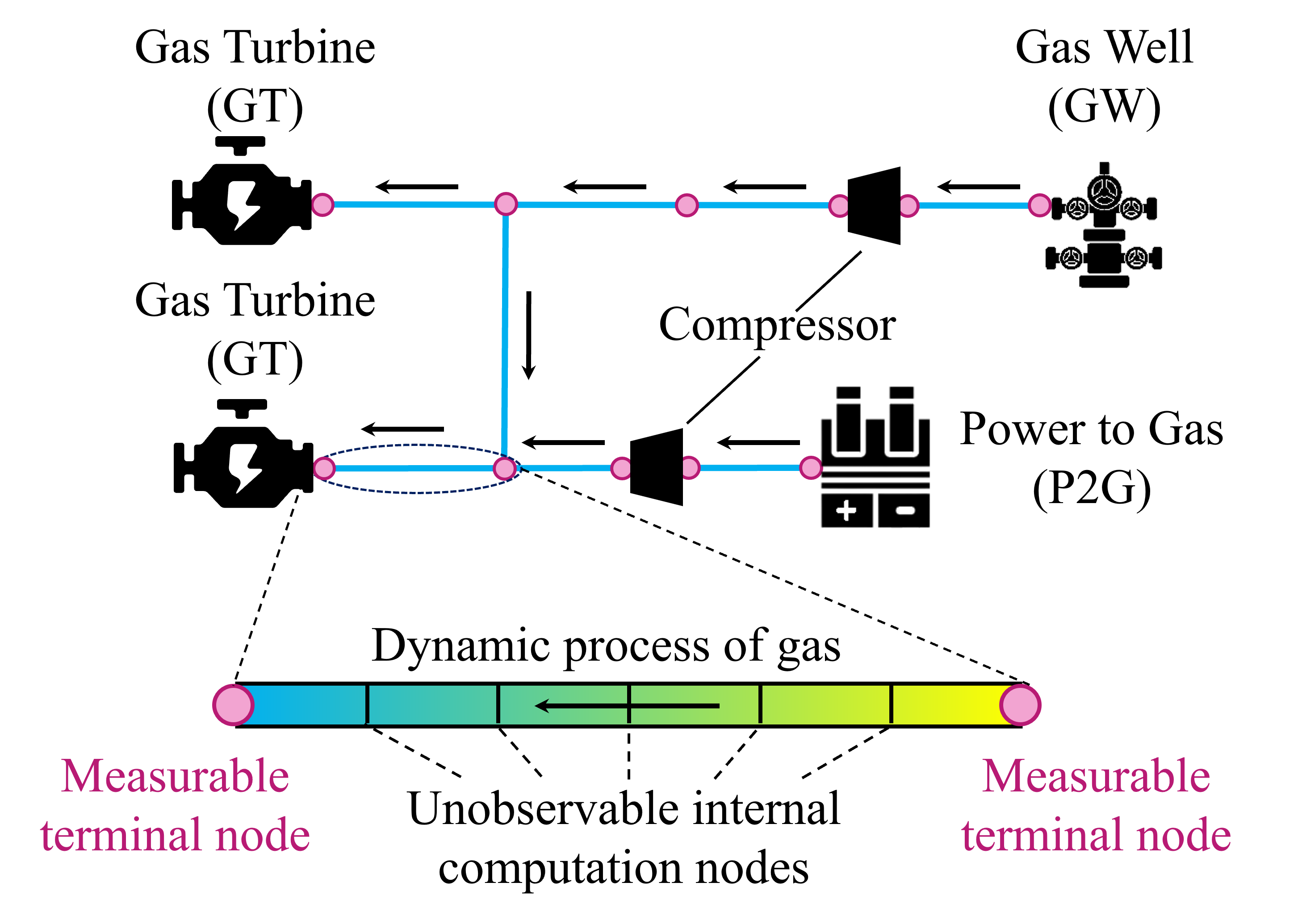
Figure 1: Schematic of the gas pipeline network and its measurement configuration

To calculate the dynamic states of a gas pipeline network for model predictive control, essential parameters include cross-sectional diameter $D$, friction coefficient $\lambda$, and pipeline length. However, discrepancies between pipeline parameters in practice and their blueprint may lead to inaccurate models [17]. Obtaining precise friction coefficients of pipelines $\lambda$ is also challenging [31]. Hence, employing a data-driven method to identify precise state-space model for the gas pipeline network through measurement operation data is necessary.

To establish the state-space model for the entire gas pipeline network, we discretize the spatial locations in the partial differential equations (1)-(2). As shown in Figure 1, to depict gas states along a pipeline, it is partitioned into equidistant discrete computation nodes. The states at internal computation nodes are unobservable; only the states at terminal nodes can be measured. Thus, we can only leverage the measurement data at terminal nodes to identify the state-space model of the entire pipeline network. Additionally, the dynamic process of gas cannot be expressed merely as a state transition function due to topological constraints inherent in the gas network, which must be maintained throughout the dynamic process. These characteristics present significant technical challenges in identifying the state-space model of the gas pipeline network.

Leveraging the memory retention feature of RNNs, this paper presents a physics-informed recurrent network model to identify the state-space model of gas pipeline network with sparse measurement data. The embedding of physics state-space model inside the recurrent network model make it physically interpretable and can be integrated into arbitrary optimal dispatch problems. A comparison between standard RNN and physics-informed recurrent network model is shown in Table 1.

To demonstrate the effectiveness of the identified state-space model, the optimal dispatch of the integrated power-gas system is implemented. By jointly optimizing the operation of generators, GTs, GWs, P2Gs and compressors, the economic benefits of the integrated system can be fully exploited.

Table 1: Comparison between Standard RNN and Physics-Informed Recurrent Network

Comparison items	Standard RNN	Physics-informed recurrent network
Input layer	Input data	Control variables order of control units in the gas system
Hidden layer	Hidden states	Internal states of unobservable computation nodes inside the pipelines
Output layer	Predict data	Predict measurable states of gas
Label	Ground truth	Measurement data of measurable variables
Composition of network	Artificial neural perceptron	Matrices in the state-space function of gas pipeline network
Trainable parameters	Dense matrix without physical meaning	Sparse matrix with specific physical meaning
Training purpose	Classification or fitting	Acquire the parameters of the state-space function
Training algorithm	Backward propagation through time (BPTT)
Implementation framework	PyTorch/TensorFlow

3 State-Space Model Identification of Gas Pipeline Network

3.1 Mathematical Model of Gas Pipeline Network

To derive a more practical state-space model of a gas pipeline network, simplify and discrete the fluid partial differential equations (1)-(2) and supplement the topology constraints of the whole network.

The convective term in (2) can be approximately considered as 0 [30, 32] and the inclination angle $\alpha$ can also be set to zero, that is

$$\frac{\partial\rho v^{2}}{\partial x}\approx 0$$ (3)

$$\sin\alpha=0$$ (4)

The Taylor expansion method is adopted [33] for the quadratic term of speed in (2), that is:

$$v^{2}\approx 2v_{b}v-v_{b}^{2}$$ (5)

where $v_{b}$ denotes the base value of gas velocity.

Besides, the physical variables gas pressure $\pi$ and mass flow $f$ are usually used to represent the state of gas pipeline.

$$\pi\approx u^{2}\rho$$ (6)

$$f=\rho vA$$ (7)

where $u$ denotes the speed of sound; $A$ denotes the cross-section area of pipeline. Equation (6) holds under approximately adiabatic condition.

Finally, based on the approximation in (3)-(5) and the variables replacement in (6)-(7), the partial differential equations (1)-(2) are transformed into

$$\frac{\partial\pi}{\partial t}=-\frac{u^{2}}{A}\frac{\partial f}{\partial x}$$ (8)

$$\frac{\partial f}{\partial t}=-A\frac{\partial\pi}{\partial x}-\frac{\lambda v_{b}}{D}f+\frac{\lambda Av_{b}^{2}}{2u^{2}D}\pi$$ (9)

Then, the partial differential equations can be discretized in the implicit upwind scheme. For any $l\in\mathcal{L}$ and $i\in\mathcal{S}_{l}$

$$\pi_{i,t}+\frac{u^{2}\Delta t}{A_{l}\Delta x_{l}}f_{i,t}-\frac{u^{2}\Delta t}{A_{l}\Delta x_{l}}f_{i-1,t}=\pi_{i,t-1}$$ (10)

$$\left(1+\frac{\lambda_{l}v_{b,l}\Delta t}{D_{l}}\right)f_{i,t}-\frac{A_{l}\Delta t}{\Delta x_{l}}\pi_{i-1,t}+\left(\frac{A_{l}\Delta t}{\Delta x_{l}}-\frac{\lambda_{l}A_{l}v_{b,l}^{2}\Delta t}{2u^{2}D_{l}}\right)\pi_{i,t}=f_{i,t-1}$$ (11)

where $\mathcal{L}$ and $\mathcal{S}$ denote the index set of pipelines and computation nodes, respectively; $\mathcal{S}_{l}$ denotes the index set of computation node in the pipeline $l$. For the convenience of numerical computation, each pipeline is divided to sections by several computation nodes.

There are also topology constraints in the gas network. First, the gas pressures of terminal segments are equal to the pressure of terminal node. Denote $\mathcal{N}$ as the index set of terminal nodes. For any $n\in\mathcal{N}$

$$\pi_{i,t}=\pi_{n,t}^{\mathrm{node}},i\in\mathcal{S}_{n}$$ (12)

where $\pi_{n,t}^{\mathrm{node}}$ denotes the gas pressure of terminal node $n$ at time $t$; $\mathcal{S}_{n}$ denotes the index set of computation nodes coincident with the terminal node $n$. $\pi_{i,t}$ denotes the gas pressure of computation node $i$ at time $t$.

Then, the sum of mass flow into the node equals the sum of mass flow out of the terminal node. For any $n\in\mathcal{N}$

$$\sum_{i\in\mathcal{S}_{n}^{+}}f_{i,t}+f_{n,t}^{\mathrm{inj}}=\sum_{j\in\mathcal{S}_{n}^{-}}f_{j,t}$$ (13)

where $\mathcal{S}_{n}^{+}$ and $\mathcal{S}_{n}^{-}$ denote index set of computation nodes that flow into and out of the terminal node, respectively; $f_{n,t}^{\mathrm{inj}}$ denotes the mass flow injection into node $n$ at time $t$; $f_{i,t}$ denotes the mass flow of computation node $i$ at time $t$.

The compressors are used to boost the gas pressure. For any $k\in\mathcal{D}^{\mathrm{comp}}$

$$\pi_{j,t}=\pi_{i,t}+\Delta\pi_{k,t},i\in\mathcal{S}_{k}^{+},j\in\mathcal{S}_{k}^{-}$$ (14)

where $\mathcal{D}^{\mathrm{comp}}$ denotes the index set of compressors; $\mathcal{S}_{k}^{+}$ and $\mathcal{S}_{k}^{-}$ denote the index of computation node flowing into and out the compressor $k$, respectively; $\Delta\pi_{k,t}$ denotes the boosted gas pressure provided by compressor $k$ at time $t$.

3.2 State-space Model of Gas Pipeline Network

In the gas pipeline network, gas pressure and mass flow rate are two variables representing the state at each computation node. Besides, the states inside the pipelines are unobservable, while the states at terminal nodes are measurable or controllable [34]. For example, the gas pressure at the gas source node is controllable and the injection gas mass flow rate at the gas consumption node is controllable. The other terminal nodes without gas injection are classified as injection gas mass flow rate measurable, since their gas injections are specified as 0. Denote $\mathcal{N}_{\pi}$ and $\mathcal{N}_{f}$ as the index set of terminal nodes whose gas pressure and gas injection mass flow rate are measured, respectively. Then, the variables in the gas system can be classified into three types: the control variables $\bm{u}_{t}$, measurable variables $\bm{y}_{t}$ and state variables $\bm{h}_{t}$, whose definitions are shown as follows:

$$\bm{u}_{t}:=\underset{n\in\mathcal{N}}{\operatorname{col}}\left(u_{n,t}\right),u_{n,t}:=\left\{\begin{array}[]{c}\pi_{n,t}^{\mathrm{node}},n\in\mathcal{N}_{\pi}\\ f_{n,t}^{\mathrm{inj}},n\in\mathcal{N}_{f}\end{array}\right.$$ (15)

$$\bm{y}_{t}:=\underset{n\in\mathcal{N}}{\operatorname{col}}\left(y_{n,t}\right),y_{n,t}:=\left\{\begin{array}[]{c}\pi_{n,t}^{\mathrm{node}},n\in\mathcal{N}_{f}\\ f_{n,t}^{\mathrm{inj}},n\in\mathcal{N}_{\pi}\end{array}\right.$$ (16)

$$\bm{h}_{t}:=\left[\bm{\pi}_{t}^{\top},\bm{f}_{t}^{\top}\right]^{\top},\bm{\pi}_{t}:=\underset{i\in\mathcal{S}}{\operatorname{col}}\left(\pi_{i,t}\right),\bm{f}_{t}:=\underset{i\in\mathcal{S}}{\operatorname{col}}\left(f_{i,t}\right)$$ (17)

where the operator $\operatorname{col}(\cdot)$ denotes the column vector operator.

Based on the discretized partial differential equations (10)-(11), the topology constrains (12)-(13) and compressor model (14), the state-space model of the whole gas system can be denoted as the compact matrix form:

$$\bm{K}(\bm{\theta})\left[\begin{array}[]{c}\bm{h}_{t}\\ \bm{\pi}_{t}^{\mathrm{node}}\end{array}\right]=\left[\begin{array}[]{c}\bm{S}\bm{h}_{t-1}\\ \bm{u}_{t}\end{array}\right]$$ (18)

$$\bm{y}_{t}=\bm{H}\bm{h}_{t}$$ (19)

where $\bm{K}(\bm{\theta})$ denotes a sparse matrix with the unknown parameters $\bm{\theta}$ to be identified; $\bm{h}_{t}$ denotes the vector collecting all the state variables at time $t$; $\bm{\pi}_{t}^{\mathrm{node}}$ denotes the vector composed of the gas pressure at each terminal node at time $t$; $\bm{u}_{t}$ denotes the vector composed of the control variables at each node and the gas pressure increment of compressors at time $t$; $\bm{S}$ is a constant matrix used to rearrange and select the elements in $\bm{h}_{t-1}$. $\bm{H}$ is also a constant matrix used to calculate the measurable output variables based on the state variables according to the topology constraints. The method to construct $\bm{S}$ and $\bm{H}$ can be clearly seen in the following small case.

To demonstrate the construction of state-space model, we use a 3-node small gas system as an example, as shown in Figure 2. Each pipeline is divided into 2 segments and there are total of 6 computation points, numbered $1^{\prime}$-$6^{\prime}$ , respectively.

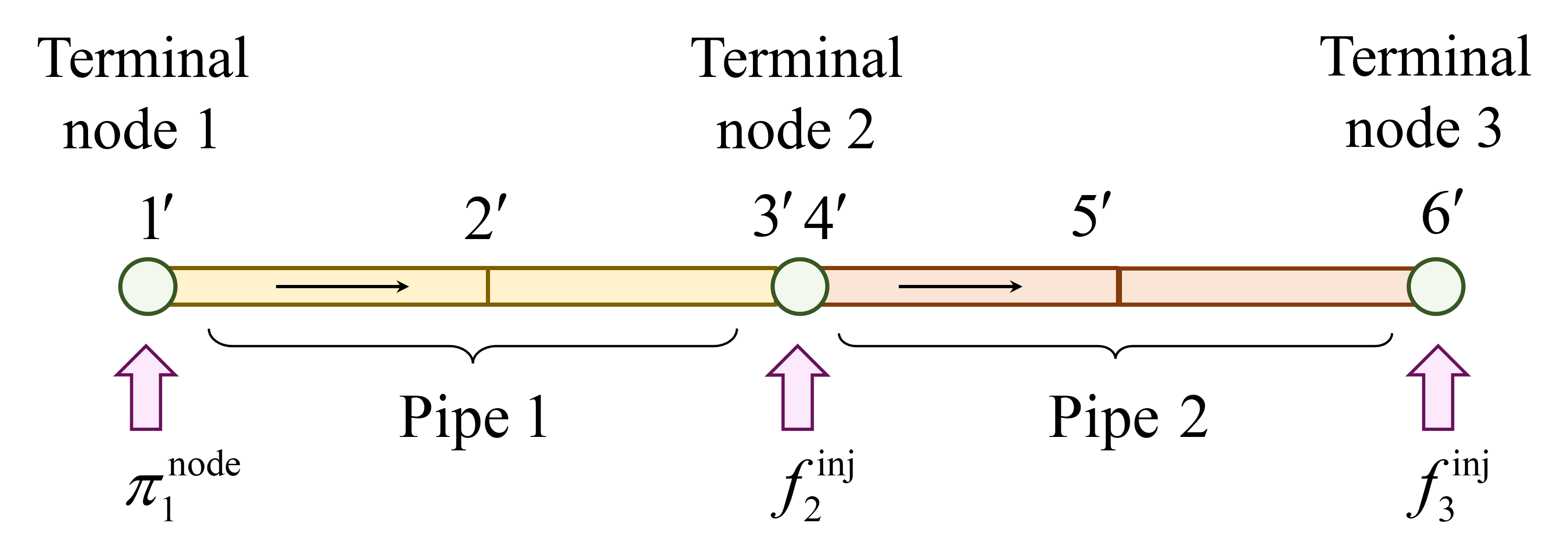
Figure 2: Topology of the 3-node small gas system.

Suppose the gas pressure at terminal node 1 is controllable, and the injection mass flow rates at terminal node 2 and 3 are controllable. Then, the control variable vector $\bm{u}_{t}$ is

$$\bm{u}_{t}:=\left[\pi_{1,t}^{\mathrm{node}},f_{2,t}^{\mathrm{inj}},f_{3,t}^{\mathrm{inj}}\right]^{\top}$$ (20)

The dynamic function (18) of this 3-node simple gas system can be written in the following matrix form as shown in Figure 3.

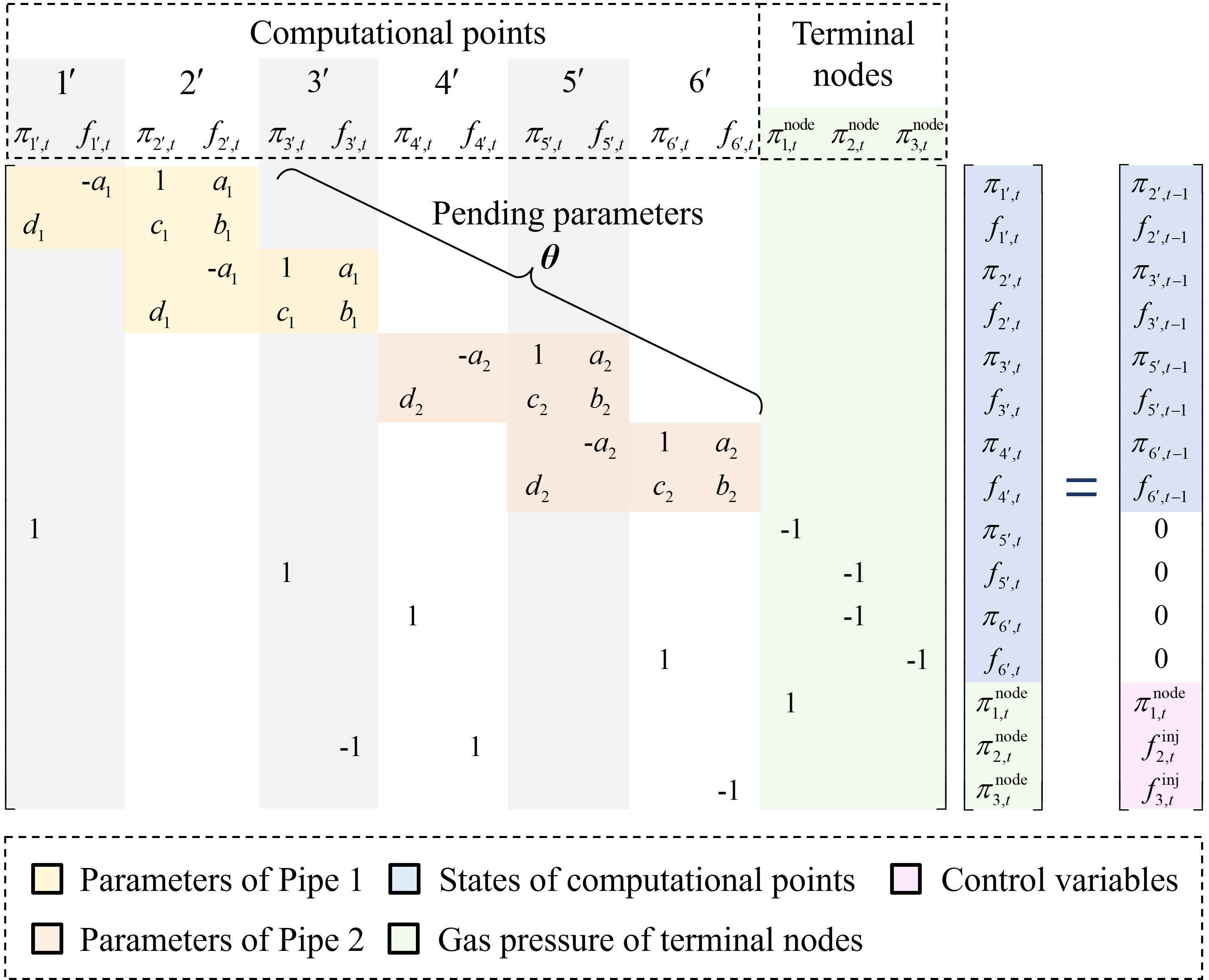
Figure 3: Matrix dynamic function of the 3-node gas system.

The detail parameters inside the sparse matrix are as follows:

$$a_{l}:=\frac{u^{2}\Delta t}{A_{l}\Delta x_{l}},b_{l}:=\left(1+\frac{\lambda_{l}v_{b,l}\Delta t}{D_{l}}\right)$$ (21)

$$c_{l}:=\left(\frac{A_{l}\Delta t}{\Delta x_{l}}-\frac{\lambda_{l}A_{l}v_{b,l}^{2}\Delta t}{2u^{2}D_{l}}\right),d_{l}:=-\frac{A_{l}\Delta t}{\Delta x_{l}}$$

$$l\in\mathcal{L}=\{1,2\}$$

In this case, the parameters $\bm{\theta}$ to be identified, the vector of state variables $\bm{h}_{t}$, the vector of gas node pressure $\bm{\pi}_{t}^{\mathrm{node}}$ and the measurable output variable vector $\bm{y}_{t}$ are shown as follows:

$$\bm{\theta}:=\underset{l\in\mathcal{L}}{\operatorname{col}}\left(\bm{\theta}_{l}\right),\bm{\theta}_{l}:=\left[a_{l},b_{l},c_{l},d_{l}\right]^{\top}$$ (22)

$$\bm{h}_{t}:=\left[\begin{array}[]{l}\pi_{1^{\prime},t},f_{1^{\prime},t},\pi_{2^{\prime},t},f_{2^{\prime},t},\pi_{3^{\prime},t},f_{3^{\prime},t},\\ \pi_{4^{\prime},t},f_{4^{\prime},t},\pi_{5^{\prime},t},f_{5^{\prime},t},\pi_{6^{\prime},t},f_{6^{\prime},t}\end{array}\right]^{\top}$$ (23)

$$\bm{\pi}_{t}^{\mathrm{node}}:=\left[\pi_{1,t}^{\mathrm{node}},\pi_{2,t}^{\mathrm{node}},\pi_{3,t}^{\mathrm{node}}\right]^{\top}$$ (24)

$$\bm{y}_{t}:=\left[f_{1,t}^{\mathrm{inj}},\pi_{2,t}^{\mathrm{node}},\pi_{3,t}^{\mathrm{node}}\right]^{\top}$$ (25)

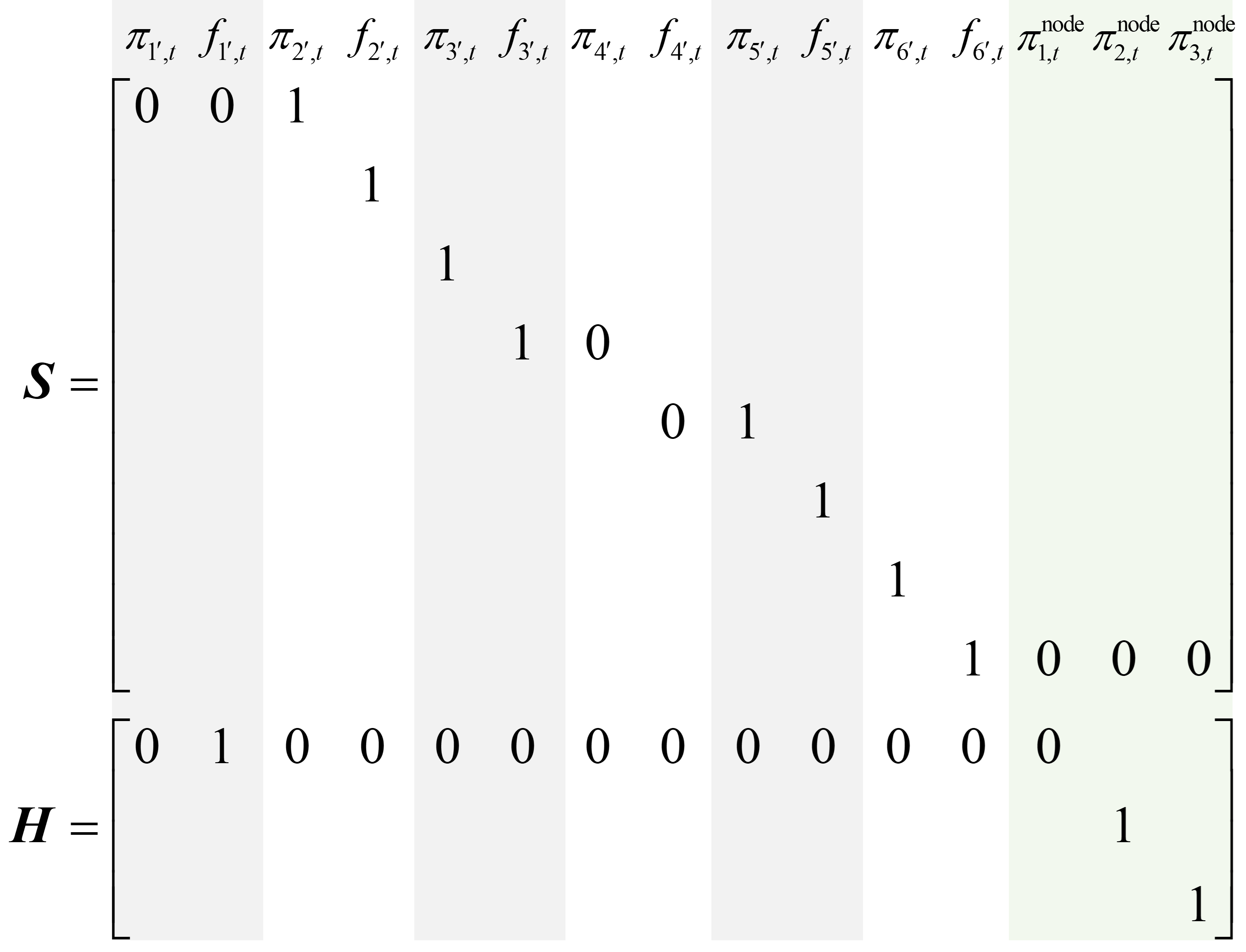
Figure 4: Values of matrices in the 3-node gas system.

According to the matrix dynamic function in Figure 4, to calculate the state variables $\bm{h}_{t}$, it only needs the values in $\bm{h}_{t-1}$ that start from the second computation points. This is because the state of the first computation points of each pipeline ($1^{\prime}$ and $4^{\prime}$ in this case) are not independent. Their values are also determined by topology constraints at terminal nodes. The constant matrix $\bm{S}$ is used to select the independent states from all state variables. In this small case, the value of matrices $\bm{S}$ and $\bm{H}$ are shown in Figure 4.

3.3 Identify the State-Space Model with Physics-Informed Recurrent Network

This subsection introduces the state-space model of the pipelines using the measurement data in the dynamic process. A novel physics-informed recurrent network is proposed to identify the parameters in the state-space model (18)-(19).

The sparse matrix $\bm{K}(\bm{\theta})$ is composed of the dynamic equations (10) and (11), along with the network topology constraints. As a result, it forms a full-rank, invertible matrix. Let the inverse of matrix $\bm{K}(\bm{\theta})$ be denoted as $\bm{J}$, and divide it into four blocks. Then, equation (18) can be transformed into:

$$\left[\begin{array}[]{c}\bm{h}_{t}\\ \bm{\pi}_{t}^{\mathrm{node}}\end{array}\right]=\left[\begin{array}[]{ll}\bm{J}^{(1)}&\bm{J}^{(2)}\\ \bm{J}^{(3)}&\bm{J}^{(4)}\end{array}\right]\left[\begin{array}[]{c}\bm{S}\bm{h}_{t-1}\\ \bm{u}_{t}\end{array}\right]$$ (26)

Base on the state transition equation (26) and the output equation (19), the diagram of physics-informed recurrent network model training architecture is shown in Figure 5. The control variables $\bm{u}_{t}$ are inputs of this system. The state variables $\bm{h}_{t}$ updates based on the input variables and the previous state $\bm{h}_{t-1}$. The outputs $\hat{\bm{y}}_{t}$ are the predicted output data and the labels $\bm{y}_{t}$ are the real measured states.

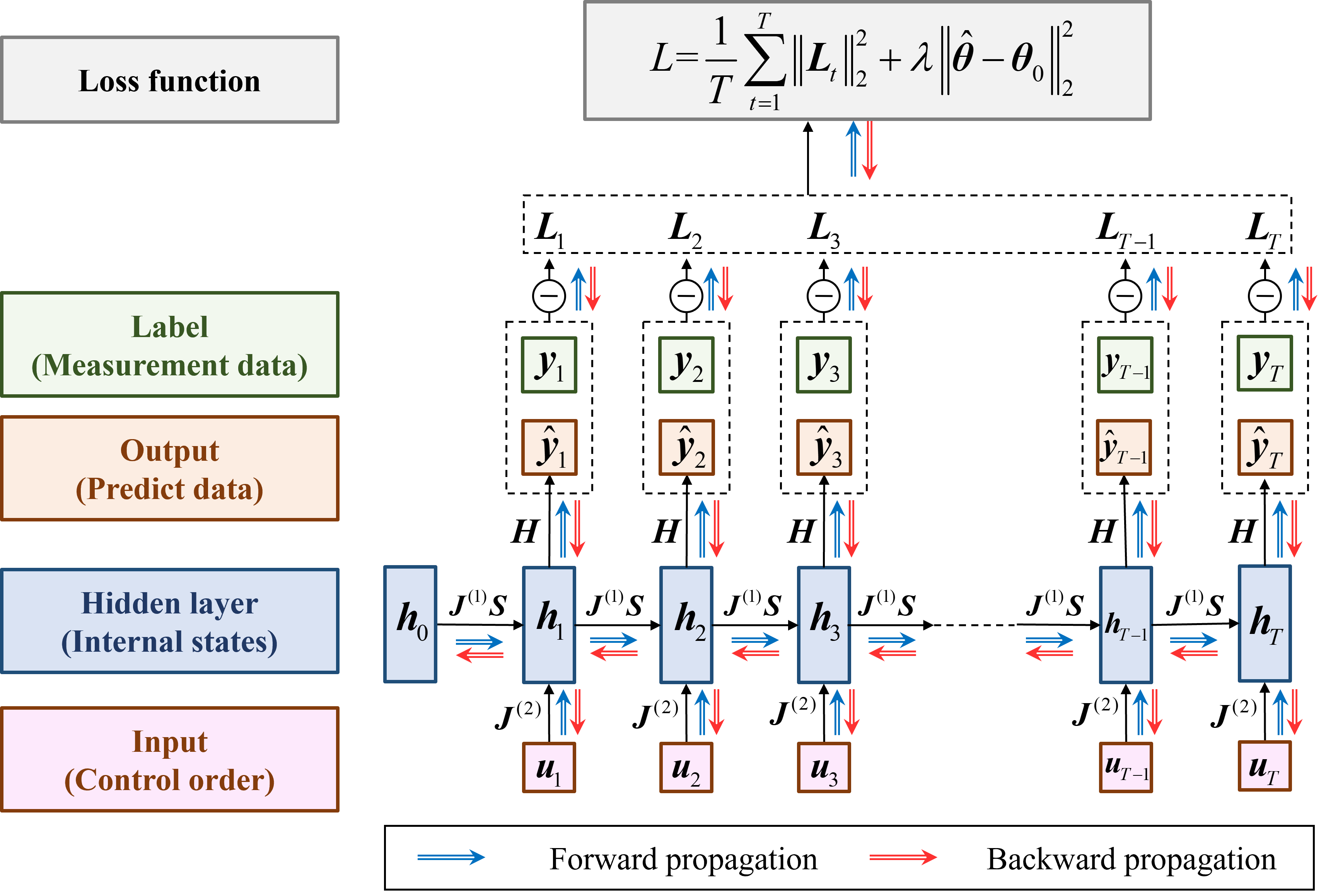
Figure 5: Diagram of physics-informed recurrent network framework.

The loss function is

$$L=\frac{1}{T}\sum_{t=1}^{T}\left\|\bm{L}_{t}\right\|_{2}^{2}+\lambda\left\|\hat{\bm{\theta}}-\bm{\theta}_{0}\right\|_{2}^{2}$$ (27)

$$\bm{L}_{t}=\hat{\bm{y}}_{t}-\bm{y}_{t}$$ (28)

where $\hat{\bm{\theta}}$ denotes the pending parameters; $\bm{\theta}_{0}$ denotes the initial estimated values of parameters based on the prior knowledge of physical meaning. The second term of the loss function (27) is a regularization term of parameters, and $\lambda$ is a hyper-parameter. Usually, the final solutions obtained by the data-driven learning are not unique, because it may converge to different local optima in the gradient descent process. The regularization term in the loss function can make our training results converge to the parameters that have right physical meaning, rather than other local optima. When the order of magnitude of the estimated parameters $\bm{\theta}_{0}$ are the same as the real value, the correctness of the parameter solution can be guaranteed.

The goal of backpropagation is to determine the partial derivatives of the loss function with respect to the parameters and initial states [35], in order to minimize the error between the predicted output data and the measurement data. This allows for the subsequent update of the parameter and initial state values as follows:

$$\hat{\bm{\theta}}\leftarrow\hat{\bm{\theta}}-\alpha_{\theta}\frac{\partial L}{\partial\hat{\bm{\theta}}}$$ (29)

$$\bm{h}_{0}\leftarrow\bm{h}_{0}-\alpha_{h}\frac{\partial L}{\partial\bm{h}_{0}}$$ (30)

where $\alpha_{\theta}$ and $\alpha_{h}$ denote the learning rates of $\hat{\bm{\theta}}$ and $\bm{h}_{0}$, respectively, and they are the hyper-parameters in the model. With the PyTorch framework, we leverage automatic differentiation to compute partial derivatives numerically, facilitating backward propagation and parameter updates in (29)-(30). However, this process involves repeated inversion of the large-scale sparse matrix $\bm{K}(\hat{\bm{\theta}})$ to obtain updated $\bm{J}$ as the parameters $\hat{\bm{\theta}}$ updated, which introduces a significant computational burden and can lead to numerical instability. To address this issue, we apply the matrix inversion lemma to update the new value of the matrix $\bm{J}$. When the parameters $\hat{\bm{\theta}}$ inside the sparse matrix $\bm{K}(\hat{\bm{\theta}})$ change to $\hat{\bm{\theta}}+\Delta\hat{\bm{\theta}}$, the matrix update can be denoted as:

$$\Delta\bm{K}:=\bm{K}(\hat{\bm{\theta}}+\Delta\hat{\bm{\theta}})-\bm{K}(\hat{\bm{\theta}})=\bm{M}\Delta\bm{\Theta}\bm{N}^{\top}$$ (31)

where $\Delta\bm{\Theta}$ is a diagonal matrix. All parameters change $\Delta\hat{\bm{\theta}}$ within $\bm{K}(\hat{\bm{\theta}}+\Delta\hat{\bm{\theta}})$ are rearranged and assigned to the diagonal elements of the matrix $\Delta\bm{\Theta}$. Constant matrices $\bm{M}$ and $\bm{N}$ are employed to position the parameter changes $\Delta\hat{\bm{\theta}}$ from $\Delta\bm{\Theta}$ to $\Delta\bm{K}$ through matrix operations. Consequently, using the matrix inversion lemma, the updated matrix $J$ can be expressed as

$$\bm{J}\leftarrow(\bm{K}+\Delta\bm{K})^{-1}=\bm{J}-\bm{J}\bm{M}\bm{\Psi}\bm{N}^{\top}\bm{J}$$ (32)

$$\bm{\Psi}:=\left(\Delta\bm{\Theta}^{-1}+\bm{N}^{\top}\bm{J}\bm{M}\right)^{-1}$$ (33)

With the matrix inversion lemma, repeat calculation of large-scale sparse matrix inversion can be effectively avoided. Additionally, it offers greater numerical stability compared to directly computing the backpropagation of an inverse matrix.

3.4 Training Techniques of Physics-Informed Recurrent Network

(1) Warm start

A warm start avoids numerical instability during matrix inversion more efficiently than random initialization, as well as accelerates the training process. Since all the parameters have an explicit physical meaning, the initial values of pending parameters $\hat{\bm{\theta}}$ and initial states $\bm{h}_{0}$ can be estimated based on the prior knowledge of physical meanings. The initial value of pending parameters $\hat{\bm{\theta}}$ can be directly set as $\bm{\theta}_{0}$. The initial states $\bm{h}_{0}$ in steady state can be estimated according to the physical model of gas pipeline. According to the partial differential equations of gas pipelines, the expressions of mass flow and gas pressure distribution along the pipeline in steady state are as follows:

$$f(x)=f(0),x\in[0,L]$$ (34)

$$\pi^{2}(x)=\pi^{2}(0)-\frac{\lambda u^{2}f^{2}}{A^{2}D}x,x\in[0,L]$$ (35)

where $f(x)$ and $\pi(x)$ denote the mass flow and gas pressure at the position $x$ along the pipeline, respectively; $L$ is the total length of the pipeline. Therefore, the initial values of gas pressure $\pi^{2}(x)$ can be estimated by linear interpolation between the gas pressure at the beginning and end of the pipeline $\pi^{2}(0)$ and $\pi^{2}(L)$.

(2) Data normalization

The substantial disparities in pressure and mass flow rate within the gas network, e.g., $10^{5}$-$10^{6}$ and $10^{0}$-$10^{1}$, pose challenges for training physics-informed recurrent network model. By employing data normalization techniques, diverse physical quantities can be normalized to comparable magnitudes, ensuring numerical stability throughout the training process.

(3) Gradient clipping and truncated backward propagation through time method

Similar to the training process of the standard RNN, the backward propagation through time process also involves a chain of matrix products. High matrix powers may lead to numerical instability, causing gradients to either explode or vanish [36]. The gradient clipping method can be used to solve this problem. In each time step, the gradient is checked and forced to the upper bound or lower bound if it exceeds the limits. Besides, the truncated backward propagation through time method [35] can be applied. This method segments long-term consequences into several shorter ones, reducing the highest matrix powers, thereby enhancing model simplicity and stability.

4 Numerical Tests

4.1 Simulation Setup

The case studies are carried out on four different scales of gas network topologies from the GasLib dataset [37], including GasLib-11, GasLib-24, GasLib-40, and GasLib-135 topologies.

The programs are implemented on the Python 3.11 platform using the PyTorch framework [38]. The RMSprop optimizer is employed, with a learning rate ranging from $10^{-5}$ to $10^{-3}$, depending on the specific test cases and quality of training data. A learning rate scheduler is applied with a step size of 4, while the decay factor (gamma) is set to 0.2. The batch size is configured to 16. All models are trained on a Tesla P100 GPU with 16 GB of VRAM.

In each test case, we first set a group of parameters as the “real” parameters of pipeline network. The finite difference method (FDM) is used to simulate the operation of the gas system. The values of control variables $\bm{u}_{t}$ are then changed to simulate the dynamic process of gas in the pipeline network and the operation data of all the terminal nodes are collected as the measurement data $\bm{y}_{t}$.

4.2 Performance of Pipelines Parameters Identification

To evaluate the performance of the proposed PIRN model, the GasLib-24 system is used as a test case for identifying pipeline parameters. During the warm start process, the pipeline parameters requiring estimation are initialized with values that contain estimation errors. In this numerical test, three levels of estimation error—within the ranges of ±5%, ±15%, and ±25%—are introduced to assess the model’s performance. Random errors are added to the initial estimates within these ranges. The model is then trained for 20 epochs, using measurement data from 100 batches. At the start of each epoch, the data sequence is reshuffled to enhance learning. Figure 6 displays the identification process on a logarithmic scale for different initial estimation errors.

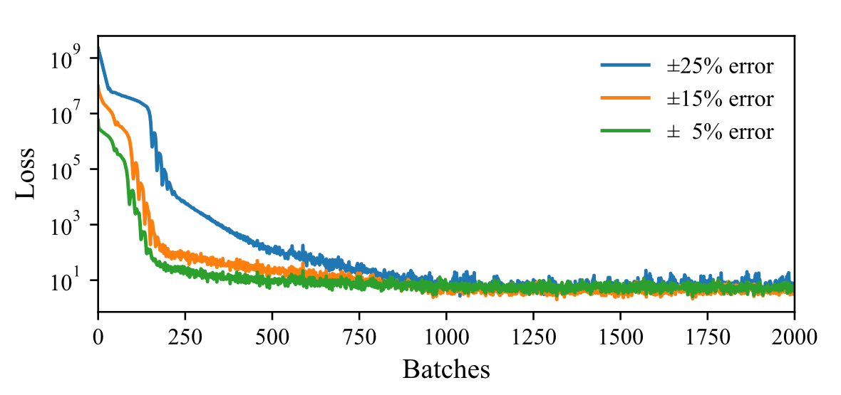
Figure 6: Parameter identification process of PIRN with different initial estimation errors.

Based on the results presented in Figure 6, the parameter identification process successfully converges across different ranges of initial estimation errors. To assess the performance of the identified state-space model for the gas pipeline network, we employed our model to compute the gas states at each node. These calculated results were then compared to the FDM simulation results. The accuracy was quantified using the mean average percentage error (MAPE) indicator, as presented in Table 2. The results demonstrate that the PIRN model effectively identifies the pipeline parameters, despite varying levels of initial estimation errors.

Table 2: Parameters Identification Results

MAPE	Ranges of initial estimation errors
	±5%	±15%	±25%
GasLib-11	0.13%	0.15%	0.16%
GasLib-24	0.12%	0.14%	0.19%
GasLib-40	0.11%	0.19%	0.21%
GasLib-135	0.09%	0.12%	0.19%

4.3 Robustness under Measurement Data with Outliers

In the PIRN model, we employ regularization, gradient clipping, mini-batch stochastic gradient descent, and learning rate scheduling techniques to mitigate the effect of measurement outliers during training. To assess its robustness, outliers with an amplitude of 15% at varying proportions are randomly introduced to simulate different noise levels in gas network data. Our parameter identification method is then applied to analyze the noise-affected data and identify gas network parameters. Figure 7 illustrates the parameter identification process of PIRN under different noise levels in the GasLib-24 system. As measurement noise deviations increase, the parameters can temporarily be trapped in local optima due to incorrect gradient descent directions affected by measurement outliers, as shown by the 5% noise curve in Figure 7. Nevertheless, the model ultimately converges after additional training iterations.

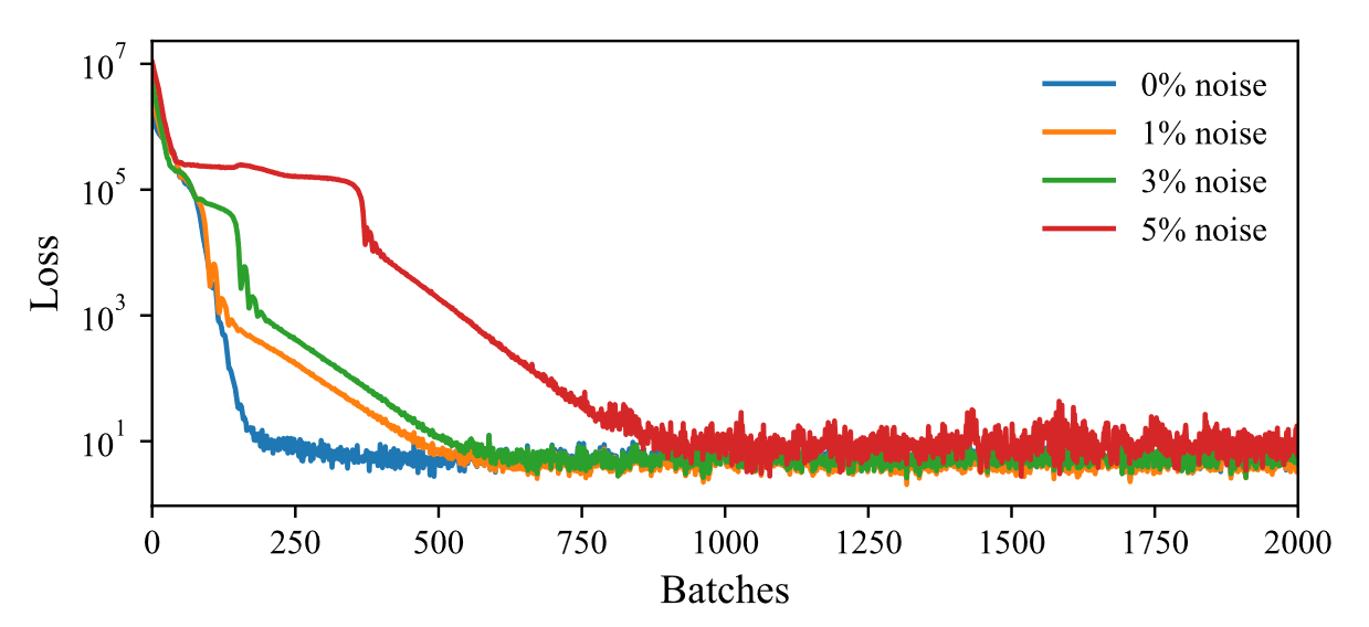
Figure 7: Parameter identification process of PIRN under different proportions of measurement outliers.

In addition, the MAPE of parameters identification results under different measurement noise with different gas pipeline network systems are listed in Table 3.

Table 3: Parameters Identification Results under Different Proportions of Outliers

MAPE	Ranges of initial estimation errors
	0%	1%	3%	5%
GasLib-11	0.11%	0.15%	0.19%	0.31%
GasLib-24	0.15%	0.17%	0.25%	0.37%
GasLib-40	0.13%	0.14%	0.24%	0.33%
GasLib-135	0.12%	0.16%	0.24%	0.35%

4.4 Parameter Efficiency Compared to Standard Neural Networks

The proposed PIRN integrates the dynamic state-space function of the gas pipeline network, resulting in a model with an explicit matrix operation form and a relatively small number of required parameters to achieve strong fitting performance. In this test case, we compare the PIRN model with the classic Elman RNN and LSTM networks. Both of these networks are trained using control variables $\bm{u}_{t}$ as inputs and measurement data $\bm{y}_{t}$ as output labels.

When all models are required to reach fitting errors within the same order of magnitude, we evaluate and compare the number of parameters necessary for each model.

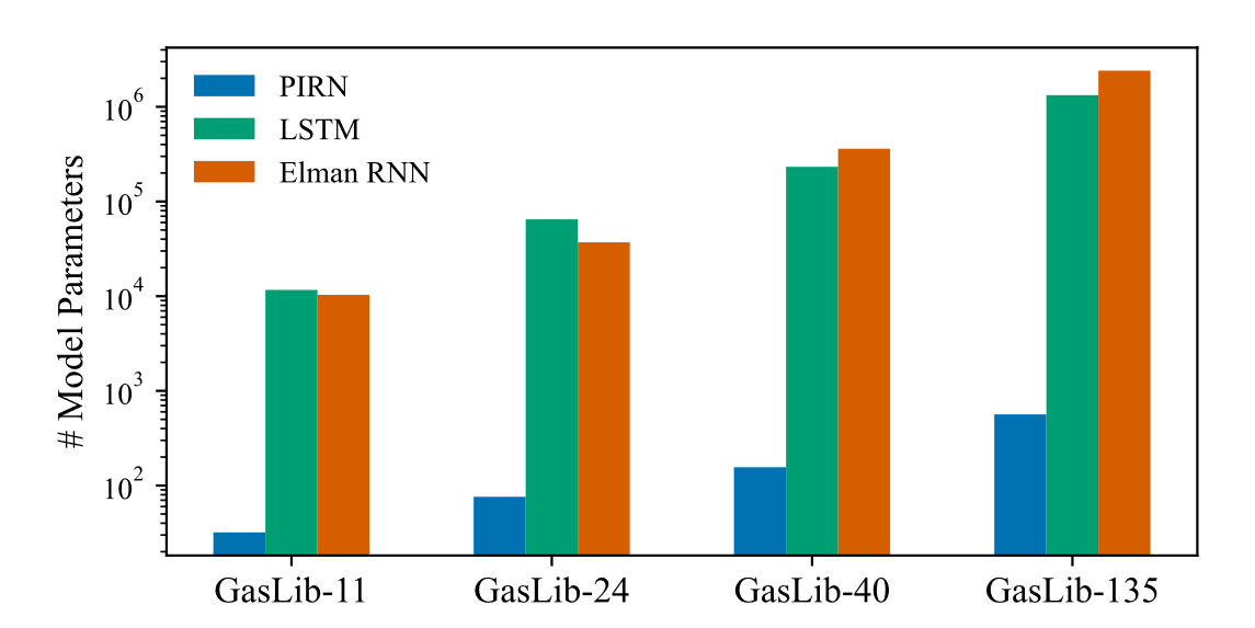
Figure 8: Number of parameters required for each model.

According to Figure 8, under the condition of achieving similar fitting accuracy, both Elman RNN and LSTM networks require significantly more parameters compared to the proposed PIRN. Moreover, as the network scale increases, this disparity becomes increasingly pronounced. Therefore, compared to RNN and LSTM networks, the proposed PIRN demonstrates better parameter efficiency compared to the standard neural networks.

4.5 Integrate the Identified State-Space Model in the Gas-Electricity Integrated Optimal Dispatch Problem

The PIRN-based parameter identification method produces an explicit state-space function for the gas pipeline network, which can directly integrate in the optimization problem. In this subsection, the IEEE RTS96 One Area 24-bus power system and the 24-pipe benchmark gas system [39] are used as numerical test cases to demonstrate how the identification results can be integrated into the optimal dispatch problem. The gas system includes 4 GTs, 4 P2Gs, and 5 compressors, while the power system consists of 1 coal generator, 3 wind turbines, and 2 photovoltaic units. Since modeling of gas-electricity integrated optimal dispatch is not the main focus of this paper, the detail descriptions of the system configurations and mathematical models can be found in the A and B, respectively. The total power system load and renewable generation curves are presented in Figure 9.

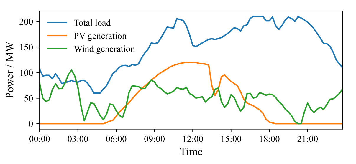
Figure 9: Total load and renewable generation curves.

Figure 10 and Figure 11 displays the gas generation curves of P2Gs and gas consumption of GTs throughout the day, respectively. During three specific timeframes (2:00-3:00, 7:00-10:00, and 11:30-13:00), the output power from renewable energy generators surpasses the total power load of the system. Consequently, P2Gs undergo electrolysis to produce natural gas for energy storage purposes. During these intervals, GTs stop gas consumption for electricity generation.

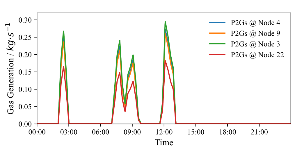
Figure 10: Gas generation of P2Gs throughout the day.

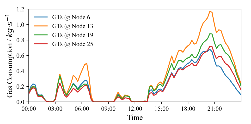
Figure 11: Gas consumption of GTs throughout the day.

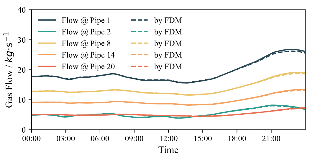
Figure 12: Gas pressures of serval terminal nodes throughout the day.

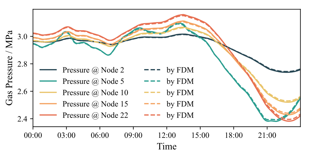
Figure 13: Gas flow rates of serval pipelines throughout the day.

Figure 12 and Figure 13 displays the gas mass flow rates in multiple pipes and the gas pressures at various nodes throughout the day, respectively. The solid lines represent our model’s calculated results, contrasting with the dashed lines reflecting outcomes from the FDM results. Then, we use the statistical indicators MAPE, RMSE and $R^{2}$ to demonstrate the performance of our method. Error statistics of gas pressure and gas mass power flow throughout the day are shown in Table 4. The identified state-space model can represent the dynamic process of the gas system with high calculation accuracy. Therefore, it can be effectively embedded in the scenarios such as optimal dispatch of integrated energy systems.

Table 4: Error Statistics of Gas Pressure and Gas Mass power Flow

Indicators	Statistics of dispatch results
	Gas pressure	Gas mass flow rate
MAPE	0.1762%	0.2131%
RMSE	0.0014 MPa	0.0374 kg/s
$R^{2}$	0.9999	0.9989

5 Conclusion

This paper introduces a physics-informed recurrent network model to identify the state-space model of the gas pipeline network using sparse measurement data from terminal nodes of pipelines. It combines data-driven learning from measurements with fluid partial differential equations governing the dynamic states of the gas pipeline network. This physics-informed recurrent network incorporates a physical embedding by substituting artificial neural perceptron units with the gas pipeline network’s physical state-space model, ensuring physical interpretability.

Utilizing the PyTorch framework, the parameters of the state-space model can be accurately learned. Case studies demonstrate that our proposed framework accurately identifies the gas pipeline network model and simultaneously estimates the internal states of gas along the pipelines. Additionally, the identified state-space model can be conveniently applied in the joint optimal dispatch of the integrated gas-electricity system problem and it performs high accuracy and parameter efficiency.

The PIRN framework uses far fewer parameters than standard neural networks, making it more sensitive to individual parameter values. This heightened sensitivity presents a challenge in quickly determining optimal hyper-parameters to improve convergence speed, requiring further exploration. Additionally, extending the PIRN framework to more complex models of gas pipeline networks, such as nonlinear models, is another important avenue for future research.

Appendix A Parameters of Numerical Tests

In our numerical tests, the IEEE RTS96 One Area 24 bus power system and 24 pipe benchmark gas system [39] are used as the gas-electricity integrated optimal dispatch test case. The parameters of GTs, P2Gs and compressors in the gas network and generators, wind turbines and photovoltaics in the power system are listed in the Table 5, 6 and 7.

Table 5: Parameters of GTs and P2Gs

Type of Units	Bus in power system	Node in gas system	Total capacity (MW)	Energy efficiency
GTs	6	8	60	0.75
GTs	13	12	80	0.77
GTs	19	18	70	0.72
GTs	25	24	60	0.69
P2Gs	4	6	8	0.48
P2Gs	9	13	7	0.44
P2Gs	3	19	9	0.50
P2Gs	22	25	6	0.54

Table 6: Parameters of Compressors

Compressors	Pipeline in gas system	Maximum additional gas pressure (MPa)	Locating distance from the head node (km)
COMP1	P1	0.1	2
COMP2	P8	0.05	5
COMP3	P3	0.03	1
COMP4	P14	0.04	3
COMP5	P20	0.06	1

Table 7: Parameters of Generators in the Power System

Type of unites	Bus in power system	Total capacity (MW)
Coal generators	2	100
Wind turbines	4	65
Wind turbines	18	80
Wind turbines	21	55
Photovoltaics	16	50
Photovoltaics	22	70

Appendix B Mathematical Model of Gas-electricity Integrated Optimal Dispatch

B.1 Models of Gas System

According to the parameter identification results, the state-space model of the gas pipeline network is as follows:

$$\bm{h}_{t}=\bm{J}^{(1)}\bm{S}\bm{h}_{t-1}+\bm{J}^{(2)}\bm{u}_{t}$$ (36)

where the matrices $\bm{J}^{(1)}$ and $\bm{J}^{(2)}$ can be obtained by the parameter identification model. $\bm{u}_{t}$ denotes the control variable vector, collecting all the controllable gas pressure and gas mass flow injection of nodes.

The gas wells (GWs) provide natural gas for the whole gas system with the upper and lower gas injection and gas pressure bounds.

$$\underline{f}_{k}^{\mathrm{gw}}\leq f_{k,t}^{\mathrm{gw}}\leq\overline{f}_{k}^{\mathrm{gw}}$$ (37)

$$\underline{\pi}_{k}^{\mathrm{gw}}\leq\pi_{k,t}^{\mathrm{gw}}\leq\overline{\pi}_{k}^{\mathrm{gw}}$$ (38)

where $\pi_{k,t}^{\mathrm{gw}}$ and $f_{k,t}^{\mathrm{gw}}$ denote the gas pressure and gas mass flow of gas well $k$ at time $t$, respectively.

The compressors also have the maximum and minimum pressure booster limits.

$$\Delta\underline{\pi}_{k}\leq\Delta\pi_{k,t}\leq\Delta\overline{\pi}_{k}$$ (39)

where $\Delta\pi_{k,t}$ denotes the boosted gas pressure of compressor $k$ at time $t$.

The gas turbines (GTs) transform the natural gas into electricity with the efficiency $\eta_{k}^{\mathrm{gt}}$. Both their gas input and the electricity output have the upper and lower bounds.

$$p_{k,t}^{\mathrm{gt}}=\eta_{k}^{\mathrm{gt}}f_{k,t}^{\mathrm{gt}}q_{L}$$ (40)

$$\underline{f}_{k}^{\mathrm{gt}}\leq f_{k,t}^{\mathrm{gt}}\leq\overline{f}_{k}^{\mathrm{gt}}$$ (41)

where $p_{k,t}^{\mathrm{gt}}$ and $f_{k,t}^{\mathrm{gt}}$ denote the generation power and gas mass flow of gas turbine $k$ at time $t$, respectively. $\eta_{k}^{\mathrm{gt}}$ denotes the efficiency of gas-power transformation. $q_{L}$ denotes the low heat value of natural gas.

The power-to-gas devices (P2Gs) transform the electricity into natural gas with the efficiency $\eta_{k}^{\mathrm{p2g}}$. Both their electricity input and gas output have the upper and lower bounds.

$$f_{k,t}^{\mathrm{p2g}}=\eta_{k}^{\mathrm{p2g}}p_{k,t}^{\mathrm{p2g}}/q_{L}$$ (42)

$$\underline{f}_{k}^{\mathrm{p2g}}\leq f_{k,t}^{\mathrm{p2g}}\leq\overline{f}_{k}^{\mathrm{p2g}}$$ (43)

where $f_{k,t}^{\mathrm{p2g}}$ and $p_{k,t}^{\mathrm{p2g}}$ denote the generated gas mass flow and power consumption of P2G $k$ at time $t$, respectively.

For the consideration of security, the gas pressures of gas pipelines also have upper and lower bounds. For any $l\in\mathcal{L}$

$$\underline{\pi}_{l}\leq\pi_{i,t}\leq\overline{\pi}_{l},\forall i\in\mathcal{S}_{l}$$ (44)

where $\pi_{i,t}$ denotes the gas pressure of gas pipeline at the discrete computation point $i$ at time $t$. $\mathcal{L}$ denotes the index set of pipelines. $\mathcal{S}_{l}$ denotes the index set of discrete computation point of pipeline $l$.

The gas injection at nodes can be described as the net injection of all the units. For any $n\in\mathcal{N}$

$$f_{n,t}^{\mathrm{inj}}=\sum_{k\in\mathcal{D}_{n}^{\mathrm{gw}}}f_{k,t}^{\mathrm{gw}}+\sum_{k\in\mathcal{D}_{n}^{\mathrm{p2g}}}f_{k,t}^{\mathrm{p2g}}-\sum_{k\in\mathcal{D}_{n}^{\mathrm{gt}}}f_{k,t}^{\mathrm{gt}}-f_{n,t}^{\mathrm{ld}}$$ (45)

where $\mathcal{D}_{n}^{\mathrm{gw}}$, $\mathcal{D}_{n}^{\mathrm{p2g}}$, and $\mathcal{D}_{n}^{\mathrm{gt}}$ denote the index sets of gas sources, P2Gs, and GTs that directly linked to node $n$, respectively. $f_{n,t}^{\mathrm{ld}}$ denotes the mass flow rate of gas load at node $n$ at time $t$. $\mathcal{N}$ denotes the index set of all pipeline nodes.

B.2 Models of Power System

In the power system, there are some units such as GTs, P2Gs, generators (GENs), wind turbines (WTs) and photovoltaics (PVs). Each type of unit has its specific active and reactive power flexibility range and can be express as a polygon. For any $s=\{\mathrm{gt,p2g,gen,wt,pv}\}$ and any $k\in\mathcal{K}^{s}$

$$\underline{p}_{k}^{s}\leq p_{k,t}^{s}\leq\overline{p}_{k}^{s}$$ (46)

$$\underline{q}_{k}^{s}\leq q_{k,t}^{s}\leq\overline{q}_{k}^{s}$$ (47)

where $\mathcal{K}^{s}$ denotes the index sets of unit $s$ in the power system. $p_{k,t}^{s}$ and $q_{k,t}^{s}$ denote the active and reactive output power of unit $k$-th at time $t$.

The ramp rate constraints should of coal generators should also be considered as follows:

$$-r_{k}^{\mathrm{gen}}\leq p_{k,t}^{\mathrm{gen}}-p_{k,t-1}^{\mathrm{gen}}\leq r_{k}^{\mathrm{gen}}$$ (48)

where $r_{k}^{\mathrm{gen}}$ denotes the ramp rates.

The network constraints of the power system restrict the active and reactive output power among all the units. Based on the linearized power flow model, the network constraints can be expressed in the compact form as follows:

$$\bm{A}_{t}^{\mathrm{ps}}\bm{x}_{t}\leq\bm{b}_{t}^{\mathrm{ps}}$$ (49)

where $\bm{A}_{t}^{\mathrm{ps}}$ and $\bm{b}_{t}^{\mathrm{ps}}$ are constant parameters representing the network constraints of the power system; $\bm{x}_{t}$ is a vector collects the active and reactive output power of all units at time $t$, that is

$$\bm{x}_{t}:=\left[\underset{s}{\operatorname{col}}\left(\underset{k\in\mathcal{K}^{\mathrm{s}}}{\operatorname{col}}\left(p_{k,t}^{s}\right)\right)^{\top},\underset{s}{\operatorname{col}}\left(\underset{k\in\mathcal{K}^{\mathrm{s}}}{\operatorname{col}}\left(q_{k,t}^{s}\right)\right)^{\top}\right]^{\top}$$ (50)

B.3 Objective Function

The objective of optimal dispatch of integrated gas-electricity system is minimizing the total cost of these two systems.

$$\min\sum_{t\in\mathcal{T}}\left(\sum_{i\in\mathcal{K}^{\mathrm{gen}}}C_{i}^{\mathrm{gen}}+\sum_{j\in\mathcal{D}^{\mathrm{gt}}}C_{j}^{\mathrm{gt}}\right)\cdot\Delta t$$ (51)

$$C_{i}^{\mathrm{gen}}=a_{i}^{\mathrm{gen}}\left(p_{i,t}^{\mathrm{gen}}\right)^{2}+b_{i}^{\mathrm{gen}}p_{i,t}^{\mathrm{gen}}+c_{i}^{\mathrm{gen}}$$ (52)

$$C_{j}^{\mathrm{gt}}=\lambda_{j}^{\mathrm{gt}}f_{j,t}^{\mathrm{gt}}$$ (53)

where $C_{i}^{\mathrm{gen}}$ and $C_{j}^{\mathrm{gt}}$ denote the fuel cost of $i$-th generator and $j$-th GT, respectively; $a_{i}^{\mathrm{gen}}$, $b_{i}^{\mathrm{gen}}$ and $c_{i}^{\mathrm{gen}}$ are coefficients of cost function of $i$-th generator. $\lambda_{j}$ are cost of natural gas of $j$-th GT. Since the renewable generators such as wind turbines and photovoltaics do not need to consume fuel, their costs are set to 0.

References

- [1] B. Liang, W. Liu, J. Zhang, Coordinated scheduling of electricity–heat–gas integrated energy system considering emerging energy conversion technologies, Energy Reports 9 (2023) 136–144. doi:10.1016/j.egyr.2023.08.059.
- [2] S. Clegg, P. Mancarella, Integrated Electrical and Gas Network Flexibility Assessment in Low-Carbon Multi-Energy Systems, IEEE Transactions on Sustainable Energy 7 (2) (2016) 718–731. doi:10.1109/TSTE.2015.2497329.
- [3] Y. Li, W. Liu, M. Shahidehpour, F. Wen, K. Wang, Y. Huang, Optimal Operation Strategy for Integrated Natural Gas Generating Unit and Power-to-Gas Conversion Facilities, IEEE Transactions on Sustainable Energy 9 (4) (2018) 1870–1879. doi:10.1109/TSTE.2018.2818133.
- [4] X. Zhang, M. Shahidehpour, A. Alabdulwahab, A. Abusorrah, Hourly Electricity Demand Response in the Stochastic Day-Ahead Scheduling of Coordinated Electricity and Natural Gas Networks, IEEE Transactions on Power Systems 31 (1) (2016) 592–601. doi:10.1109/TPWRS.2015.2390632.
- [5] T. Zhang, Z. Li, Q. Wu, S. Pan, Q. H. Wu, Dynamic energy flow analysis of integrated gas and electricity systems using the holomorphic embedding method, Applied Energy 309 (2022) 118345. doi:10.1016/j.apenergy.2021.118345.
- [6] Y. Chen, Q. Guo, H. Sun, Z. Pan, B. Chen, Generalized phasor modeling of dynamic gas flow for integrated electricity-gas dispatch, Applied Energy 283 (2021) 116153. doi:10.1016/j.apenergy.2020.116153.
- [7] P. Lan, D. Han, X. Xu, Z. Yan, X. Ren, S. Xia, Data-driven state estimation of integrated electric-gas energy system, Energy 252 (2022) 124049. doi:10.1016/j.energy.2022.124049.
- [8] M. Nakıp, O. Çopur, E. Biyik, C. Güzeliş, Renewable energy management in smart home environment via forecast embedded scheduling based on Recurrent Trend Predictive Neural Network, Applied Energy 340 (2023) 121014. doi:10.1016/j.apenergy.2023.121014.
- [9] M. Raissi, P. Perdikaris, G. Karniadakis, Physics-informed neural networks: A deep learning framework for solving forward and inverse problems involving nonlinear partial differential equations, Journal of Computational Physics 378 (2019) 686–707. doi:10.1016/j.jcp.2018.10.045.
- [10] G. E. Karniadakis, I. G. Kevrekidis, L. Lu, P. Perdikaris, S. Wang, L. Yang, Physics-informed machine learning, Nature Reviews Physics 3 (6) (2021) 422–440. doi:10.1038/s42254-021-00314-5.
- [11] B. Huang, J. Wang, Applications of Physics-Informed Neural Networks in Power Systems - A Review, IEEE Transactions on Power Systems 38 (1) (2023) 572–588. doi:10.1109/TPWRS.2022.3162473.
- [12] K. Sundar, A. Zlotnik, Dynamic State and Parameter Estimation for Natural Gas Networks using Real Pipeline System Data, in: 2019 IEEE Conference on Control Technology and Applications (CCTA), 2019, pp. 106–111. doi:10.1109/CCTA.2019.8920430.
- [13] K. Sundar, A. Zlotnik, State and Parameter Estimation for Natural Gas Pipeline Networks Using Transient State Data, IEEE Transactions on Control Systems Technology 27 (5) (2019) 2110–2124. doi:10.1109/TCST.2018.2851507.
- [14] H. Chen, D. Qi, H. Wang, Q. Zhang, Y. Bu, L. Zuo, Identification of the characteristic parameters for gas pipe sections using the maximum likelihood method and least square method, Engineering Reports 4 (3) (2022) e12471. doi:10.1002/eng2.12471.
- [15] S. Hajian, M. Hintermüller, C. Schillings, N. Strogies, A Bayesian approach to parameter identification in gas networks, Control and Cybernetics 48 (2019).
- [16] M. G. Sukharev, M. A. Kulalaeva, Identification of model flow parameters and model coefficients with the help of integrated measurements of pipeline system operation parameters, Energy 232 (2021) 120864. doi:10.1016/j.energy.2021.120864.
- [17] G. Cui, Q.-S. Jia, X. Guan, Q. Liu, Data-driven computation of natural gas pipeline network hydraulics, Results in Control and Optimization 1 (2020) 100004. doi:10.1016/j.rico.2020.100004.
- [18] Z. Cen, J. Wei, R. Jiang, A gray-box neural network-based model identification and fault estimation scheme for nonlinear dynamic systems, International journal of neural systems 23 (2013) 1350025. doi:10.1142/S0129065713500251.
- [19] J. Zheng, J. Du, Y. Liang, C. Wang, Q. Liao, H. Zhang, Deeppipe: Theory-guided LSTM method for monitoring pressure after multi-product pipeline shutdown, Process Safety and Environmental Protection 155 (2021) 518–531. doi:10.1016/j.psep.2021.09.046.
- [20] D. Zhou, X. Jia, S. Ma, T. Shao, D. Huang, J. Hao, T. Li, Dynamic simulation of natural gas pipeline network based on interpretable machine learning model, Energy 253 (2022) 124068. doi:10.1016/j.energy.2022.124068.
- [21] L. Chen, Y. Li, M. Huang, X. Hui, S. Gu, Robust Dynamic State Estimator of Integrated Energy Systems Based on Natural Gas Partial Differential Equations, IEEE Transactions on Industry Applications 58 (3) (2022) 3303–3312. doi:10.1109/TIA.2022.3161607.
- [22] Y. Chen, Y. Yao, Y. Lin, X. Yang, Dynamic state estimation for integrated electricity-gas systems based on Kalman filter, CSEE Journal of Power and Energy Systems 8 (1) (2022) 293–303. doi:10.17775/CSEEJPES.2020.02050.
- [23] L. Chen, P. Jin, J. Yang, Y. Li, Y. Song, Robust Kalman Filter-Based Dynamic State Estimation of Natural Gas Pipeline Networks, Mathematical Problems in Engineering 2021 (1) (2021) 5590572. doi:10.1155/2021/5590572.
- [24] L. Su, Z. Han, J. Zhao, W. Wang, Graph-Frequency Domain Kalman Filtering for Industrial Pipe Networks Subject to Measurement Outliers, IEEE Transactions on Industrial Informatics 20 (5) (2024) 7977–7985. doi:10.1109/TII.2024.3369715.
- [25] Y. Huang, L. Feng, Y. Liu, A Data-Driven State Estimation Framework for Natural Gas Networks With Measurement Noise, IEEE Access 11 (2023) 30888–30898. doi:10.1109/ACCESS.2023.3262415.
- [26] G. Yin, B. Chen, H. Sun, Q. Guo, Energy circuit theory of integrated energy system analysis (IV): Dynamic state estimation of the natural gas network, Proc. CSEE 40 (18) (2020) 5827–5837.
- [27] L. Su, J. Zhao, W. Wang, Hybrid physical and data driven transient modeling for natural gas networks, Journal of Natural Gas Science and Engineering 95 (2021) 104146. doi:10.1016/j.jngse.2021.104146.
- [28] X. Yin, K. Wen, W. Huang, Y. Luo, Y. Ding, J. Gong, J. Gao, B. Hong, A high-accuracy online transient simulation framework of natural gas pipeline network by integrating physics-based and data-driven methods, Applied Energy 333 (2023) 120615. doi:10.1016/j.apenergy.2022.120615.
- [29] J. Yang, N. Zhang, C. Kang, Q. Xia, Effect of Natural Gas Flow Dynamics in Robust Generation Scheduling Under Wind Uncertainty, IEEE Transactions on Power Systems 33 (2) (2018) 2087–2097. doi:10.1109/TPWRS.2017.2733222.
- [30] Y. Zhou, C. Gu, H. Wu, Y. Song, An Equivalent Model of Gas Networks for Dynamic Analysis of Gas-Electricity Systems, IEEE Transactions on Power Systems 32 (6) (2017) 4255–4264. doi:10.1109/TPWRS.2017.2661762.
- [31] Z. Marfatia, X. Li, On steady state modelling for optimization of natural gas pipeline networks, Chemical Engineering Science 255 (2022) 117636. doi:10.1016/j.ces.2022.117636.
- [32] T. Kiuchi, An implicit method for transient gas flows in pipe networks, International Journal of Heat and Fluid Flow 15 (5) (1994) 378–383. doi:10.1016/0142-727X(94)90051-5.
- [33] F. Qi, M. Shahidehpour, F. Wen, Z. Li, Y. He, M. Yan, Decentralized Privacy-Preserving Operation of Multi-Area Integrated Electricity and Natural Gas Systems With Renewable Energy Resources, IEEE Transactions on Sustainable Energy 11 (3) (2020) 1785–1796. doi:10.1109/TSTE.2019.2940624.
- [34] B. Chen, Q. Guo, G. Yin, B. Wang, Z. Pan, Y. Chen, W. Wu, H. Sun, Energy-Circuit-Based Integrated Energy Management System: Theory, Implementation, and Application, Proceedings of the IEEE 110 (12) (2022) 1897–1926. doi:10.1109/JPROC.2022.3216567.
- [35] H. Jaeger, A tutorial on training recurrent neural networks, covering BPPT, RTRL, EKF and the ”echo state network” approach, GMD-Forschungszentrum Informationstechnik 5 (1) (2002) 46.
- [36] A. Zhang, Z. Lipton, M. Li, A. J. Smola, Dive into Deep Learning, Cambridge University Press, Cambridge New York Port Melbourne New Delhi Singapore, 2024.
- [37] M. Schmidt, D. Aßmann, R. Burlacu, J. Humpola, I. Joormann, N. Kanelakis, T. Koch, D. Oucherif, M. E. Pfetsch, L. Schewe, R. Schwarz, M. Sirvent, GasLib – A Library of Gas Network Instances, Data 2 (4) (2017) article 40. doi:10.3390/data2040040.
- [38] A. Paszke, S. Gross, F. Massa, A. Lerer, J. Bradbury, G. Chanan, T. Killeen, Z. Lin, N. Gimelshein, L. Antiga, A. Desmaison, A. Kopf, E. Yang, Z. DeVito, M. Raison, A. Tejani, S. Chilamkurthy, B. Steiner, L. Fang, J. Bai, S. Chintala, PyTorch: An Imperative Style, High-Performance Deep Learning Library, in: Advances in Neural Information Processing Systems 32, Curran Associates, Inc., 2019, pp. 8024–8035.
- [39] A. Zlotnik, L. Roald, S. Backhaus, M. Chertkov, G. Andersson, Coordinated Scheduling for Interdependent Electric Power and Natural Gas Infrastructures, IEEE Transactions on Power Systems 32 (1) (2017) 600–610. doi:10.1109/TPWRS.2016.2545522.