Non-Iterative Coordination of Interconnected Power Grids via Dimension-Decomposition-Based Flexibility Aggregation

Abstract

The bulk power grid is divided into regional grids interconnected with multiple tie-lines for efficient operation. Since interconnected power grids are operated by different control centers, it is a challenging task to realize coordinated dispatch of multiple regional grids. A viable solution is to compute a flexibility aggregation model for each regional power grid, then optimize the tie-line schedule using the aggregated models to implement non-iterative coordinated dispatch. However, challenges such as intricate interdependencies and curse of dimensionality persist in computing the aggregated models in high-dimensional space. Existing methods like Fourier-Motzkin elimination, vertex search, and multi-parameter programming are limited by dimensionality and conservatism, hindering practical application. This paper presents a novel dimension-decomposition-based flexibility aggregation algorithm for calculating the aggregated models of multiple regional power grids, enabling non-iterative coordination in large-scale interconnected systems. Compared to existing methods, the proposed approach yields a significantly less conservative flexibility region. The derived flexibility aggregation model for each regional power grid has a well-defined physical counterpart, which facilitates intuitive analysis of multi-port regional power grids and provides valuable insights into their internal resource endowments. Numerical tests validate the feasibility of the aggregated model and demonstrate its accuracy in coordinating interconnected power grids.

Nomenclature

$\bm{x}^{\text{bd}}$, $\bm{x}^{\text{int}}$	Vectors composed of all the boundary variables and internal variables of all time slots.
$\mathcal{R}_{\text{H}}$	The feasible region representing all the operational constraints of a system within a high-dimensional space where all decision variables reside.
$\mathcal{R}_{\text{L}}$	The aggregated flexibility region of a system within the projected space where the boundary variables reside.
$\hat{\mathcal{R}}_{\text{L}}$	The inner-approximated aggregate flexibility region of the system, characterized by a specific shape template.
$\overline{(\cdot)},\underline{(\cdot)}$	The upper and lower limits parameters of variables.
$[n]$	The set of integers from 1 to $n$.
$\underset{i\in\mathcal{N}}{\operatorname{col}}\left(x_{i}\right)$	The column vector composed of elements $x_{i}$ for all indices $i\in\mathcal{N}$.
$\operatorname{space}(\bm{x})$	The space where the vector $\bm{x}$ resides.
$\operatorname{card}(\mathcal{T})$	The cardinality of the set $\mathcal{T}$.

I Introduction

I-A Background and Motivation

The modern power grids in China, North America and Europe are all interconnected systems. To facilitate administration and coordination, the bulk power grid is segmented into several regional power grids (RPGs) based on geographical areas, interconnected by AC and DC tie-lines [1]. The proportion of renewable energy and the varying weather conditions in various regions create complementary patterns in peak electricity supply and demand. Energy transmission through AC and DC tie-lines provides cross-regional energy support ensures stable and economic grid operations of the whole system.

However, achieving optimal coordinated dispatch across multiple RPGs presents significant challenges, as each RPG operates under its own control center. Data privacy concerns and variations in data models further complicate the coordination between these grids. In addition, the sheer volume of devices and network data makes centralized management and optimization of the entire bulk power grid impractical. A commonly adopted approach is to coordinate RPGs using a decentralized optimization framework. In this framework, the optimal dispatch problem of each RPG is treated as a sub-problem, with the overall coordination of the bulk power grid achieved through an iterative process. However, ensuring convergence in this iterative process is challenging, and identifying the causes of divergence can be difficult when it occurs. Moreover, synchronized online communication among all regional control centers is required during coordinated dispatch, which poses substantial challenges for practical engineering applications.

An effective solution to these challenges is to calculate the power transmission flexibility region of tie-lines between RPGs, which is also called tie-line security region in [2, 3]. Then the coordination of interconnected power grids can be achieved without the need for iterative coordination [4]. A schematic diagram illustrating the aggregation of regional power grids is shown in Fig. 1.

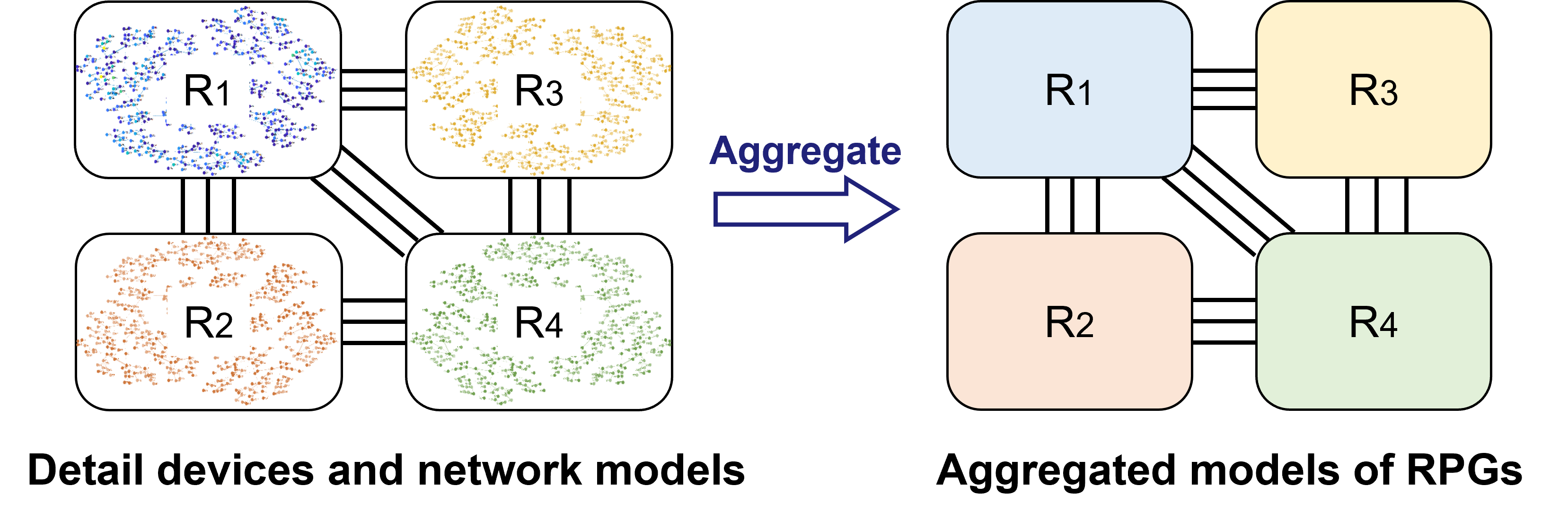
Figure 1: Aggregate the regional power grids for coordination of interconnected systems.

By employing an aggregated model, each RPG can focus solely on the external characteristics of tie-lines, without considering complex internal network constraints, thereby significantly reducing the complexity of the optimal coordination of the bulk grid. The flexibility aggregation results can also be used as a comprehensive assessment of the overall RPG, providing valuable insights for the resource endowment inside. At the same time, device data and information within each RPG is effectively protected through aggregation.

Calculating the aggregated model of an RPG still faces major challenges. Firstly, the decision variables in an RPG are numerous. All these variables are coupled with each other by large-scale spatio-temporal coupling constraints, including the network constraints at single time slices, and the temporal coupling constraints of generation units across all time slots. All the variables and the coupling constraints form a very complex high-dimensional space. Besides, an RPG connects to other RPGs through multiple AC and DC tie-lines, which are coupled with each other due to the network constraints. It is also difficult to explicitly express these spatio-temporal coupling relationships as constraints among these tie-lines.

Some existing studies have proposed several types of methodologies for computing the flexibility aggregation model of a system. The Fourier-Motzkin elimination method is proposed in [5, 6] to calculate the flexibility set of power system by eliminating the internal variables of the system. The concept of dispatchable region is presented in [7] and calculated by iteratively creating boundary hyperplanes of the feasible region. The progressive vertex enumeration method is proposed in [8] to calculate the projected flexibility region of power system by iteratively searching the extreme points. Besides, the work in [2] presents an evaluation method for the secure region of a single tie-line between regional power grids. The multi-parameter programming based algorithms are presented in [9] and its enhanced acceleration algorithm is proposed in [10]. Security region of renewable energy integration is calculated in [11] with multi-parameter programming. Geometry-based methods also offer an approach to calculate the aggregation model, where the aggregated flexibility region is approximated using various geometric shapes, such as cubes [12], ellipsoids [13], and polytopes shaped by storage and/or generator constraints [14, 15, 16]. Moreover, to deal with the high-dimension coupling among multiple tie-lines in an RPG, [3] decomposes the flexibility region along the temporal dimension and recombines the lower-dimensional regions with Cartesian product.

In practical power grids, the presence of multiple tie-lines between regional grids creates a multi-port system, significantly increasing computational complexity. Existing methods such as Fourier-Motzkin elimination, vertex search, multi-parameter programming, and direct geometric projection all suffer from the curse of dimensionality. As a result, these approaches often fail to compute the flexibility region of RPGs within a limited time, limiting their practical application in engineering. Furthermore, existing methods exhibit excessive conservatism, producing flexibility regions that are much smaller than the actual regions. This limitation prevents them from achieving optimal solutions in dispatch applications and hinders their ability to attain economic optimality.

I-B Contributions and Paper Organization

This paper proposed a novel dimension-decomposition-based inner approximation method to calculate the flexibility aggregation model of a regional power grid with multiple AC and DC tie-lines. The aggregated model integrates the network constraints, devices constraints, $N$-1 security constraints, and the capability of generators within each regional power grid. With the flexibility aggregation model of regional power grids, it can greatly simplify and accelerate the schedule of tie-lines and coordination of interconnected regional power grids in a non-iterative way.

The contributions of this paper are outlined as follows:

(1) A flexibility aggregation model is developed for each regional power grid in the bulk power system, incorporating network constraints, device constraints, and $N$-1 security constraints. These aggregated models significantly simplify and accelerate the scheduling of tie-lines, and facilitate the coordination of interconnected power grids using a non-iterative approach.

(2) A novel dimension-decomposition-based flexibility aggregation algorithm is proposed to calculate the flexibility region of each regional power grid. This method not only accelerates the computation process, making the high-dimensional problem tractable, but also achieves substantially less conservative flexibility aggregation results compared to existing approaches.

(3) The derived flexibility aggregation model of each regional power grid has a well-defined physical counterpart, which facilitates intuitive analysis of multi-port regional power grids and provides valuable insights into their internal resource endowments.

The remainder of this paper is organized as follows. Section II provides an interpretation and methodology for the flexibility aggregation problem. Section III introduces the mathematical model for a regional power grid. In Section IV, the dimension-decomposition-based inner approximation algorithm is presented to calculate the flexibility aggregation model. Physical interpretation of the flexibility aggregation model is also given. Section V describes the coordinated dispatch model of interconnected RPGs based on the aggregated flexibility results. Numerical tests are conducted in Section VI, followed by conclusions in Section VII.

II Preliminaries: Interpretation and Methodology for the Flexibility Aggregation

II-A Physical and Mathematical Interpretation for the Flexibility Aggregation Problem

System flexibility is defined as the capacity to maintain a secure and cost-effective supply-demand balance across spatial and temporal scales, achieved through the seamless coordination of various controllable assets [17, 18]. The flexibility aggregation of a system can be viewed from both the mathematical and physical perspectives, as shown in Fig. 2.

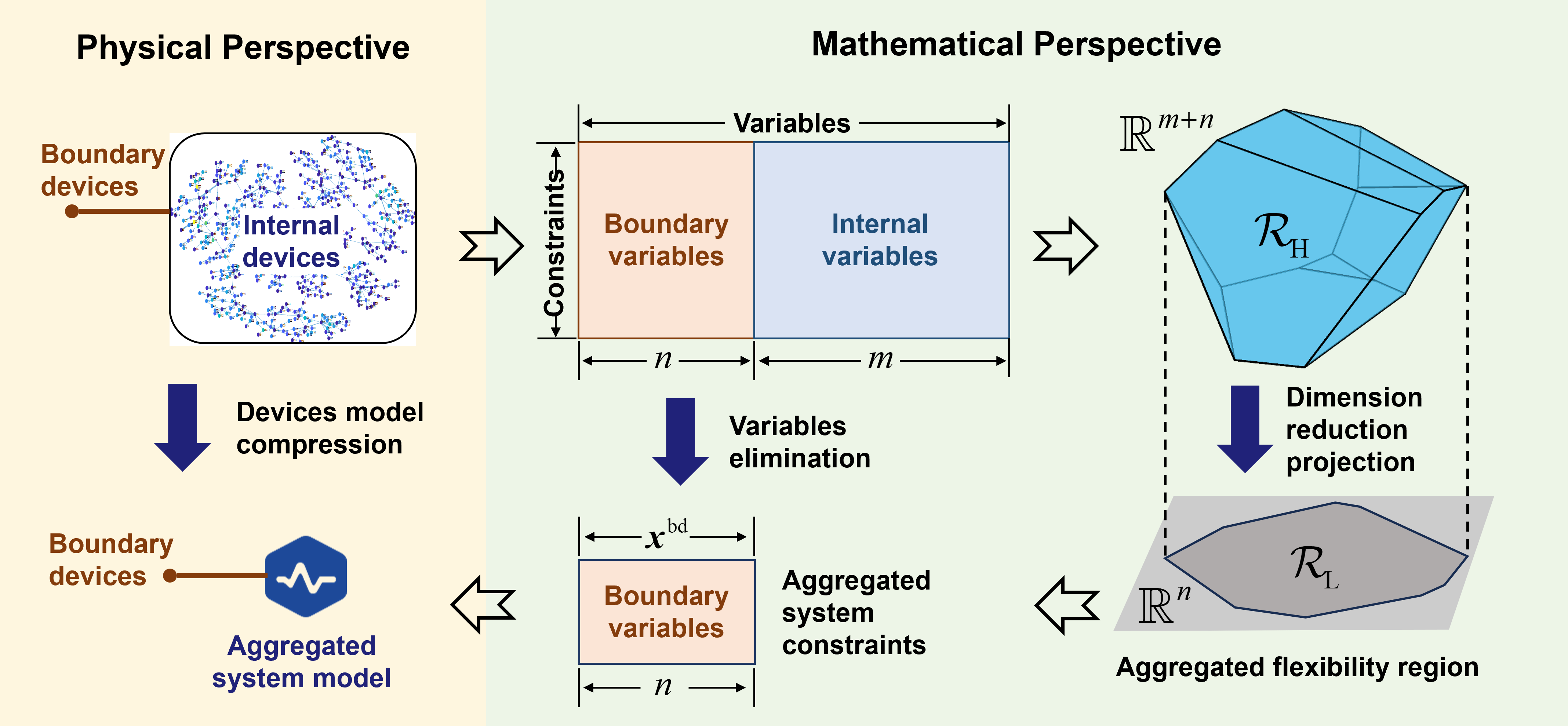
Figure 2: Physical and mathematical perspectives of system flexibility aggregation.

From a physical perspective, a system consists of numerous interconnected internal devices. These devices influence each other and interact with the external environment through boundary devices, such as feeders or tie-lines, enabling energy and information exchange. To aggregate the flexibility of the entire energy system, the internal devices and coupling networks are compressed into a flexible equivalent aggregation model. Then, the system’s overall flexibility, viewed externally, can be represented solely by the boundary devices. The internal structure of this system is treated as a black box [19].

Considering the mathematical model of all devices in the system, the system is governed by the operational and security constraints involving the internal variables $\bm{x}^{\text{int}}\in\mathbb{R}^{m}$ and the boundary variables $\bm{x}^{\text{bd}}\in\mathbb{R}^{n}$. If these constraints can be approximated or relaxed in a linear form, they constitute the feasible region $\mathcal{R}_{\text{H}}$ of the whole system as follows:

$$\mathcal{R}_{\text{H}}=\left\{\left[\begin{array}[]{l}\bm{x}^{\text{bd}}\\ \bm{x}^{\text{int}}\end{array}\right]\left\lvert\,\begin{array}[]{l}\bm{x}^{\text{bd}}=\bm{C}\bm{x}^{\text{int}}+\bm{d}\\ \bm{F}\bm{x}^{\text{int}}\leq\bm{f}\end{array}\right.\right\}$$ (1)

$\mathcal{R}_{\text{H}}$ can also be viewed as a polytopal region in the high-dimensional space $\mathbb{R}^{m+n}$. To aggregate the flexibility of the system, all internal variables $\bm{x}^{\text{int}}$ should be eliminated from the constraints of the system, so that the aggregated flexibility region can be expressed only by the constraints of the boundary variables $\bm{x}^{\text{bd}}$. From a geometric perspective, this is equivalent to the projection of the polytope $\mathcal{R}_{\text{H}}$ onto the lower-dimensional space $\mathbb{R}^{n}$, where the boundary variables $\bm{x}^{\text{bd}}$ reside:

$$\mathcal{R}_{\text{L}}=\left\{\bm{x}^{\text{bd}}\left\lvert\ \begin{array}[]{l}\forall\bm{x}^{\text{bd}}\in\mathcal{R}_{\text{L}},\exists\bm{x}^{\text{int}}:\\ \left[\begin{array}[]{l}\bm{x}^{\text{bd}}\\ \bm{x}^{\text{int}}\end{array}\right]\in\mathcal{R}_{\text{H}}\end{array}\right.\right\}$$ (2)

Since the dimensionality reduction projection of a polytope can retain the form of polytope, the projected polytope can be expressed as

$$\mathcal{R}_{\text{L}}=\left\{\bm{x}^{\text{bd}}\left\lvert\ \bm{M}^{*}\bm{x}^{\text{bd}}\leq\bm{n}^{*}\right.\right\},\mathcal{R}_{\text{L}}\subset\mathbb{R}^{n}$$ (3)

where matrix $\bm{M}^{*}$ and vector $\bm{n}^{*}$ are obtained by projection operation. However, the system’s large number of decision variables creates a high-dimensional space, leading to an over-exponential increase in computational complexity and rendering the problem NP-hard [20, 16]. Consequently, precise calculation methods to obtain exact values of $\bm{M}^{*}$ and $\bm{n}^{*}$, such as Fourier-Motzkin elimination [5] and polytope projection algorithms, become intractable.

The commonly used approaches are to calculate the inner-approximated the projected flexibility region $\mathcal{R}_{\text{L}}$ [12, 13, 15, 3, 16, 4, 21]. Denote the inner-approximated aggregated flexibility region as $\hat{\mathcal{R}_{\text{L}}}$, such that $\hat{\mathcal{R}_{\text{L}}}\subseteq\mathcal{R}_{\text{L}}$. For every dispatch order of the boundary variables $\bm{x}^{\text{bd}}$ in $\hat{\mathcal{R}_{\text{L}}}$, there exists at least one realization of the internal variables $\bm{x}^{\text{int}}$ that satisfies the system’s operation constraints, as shown in Fig. 3

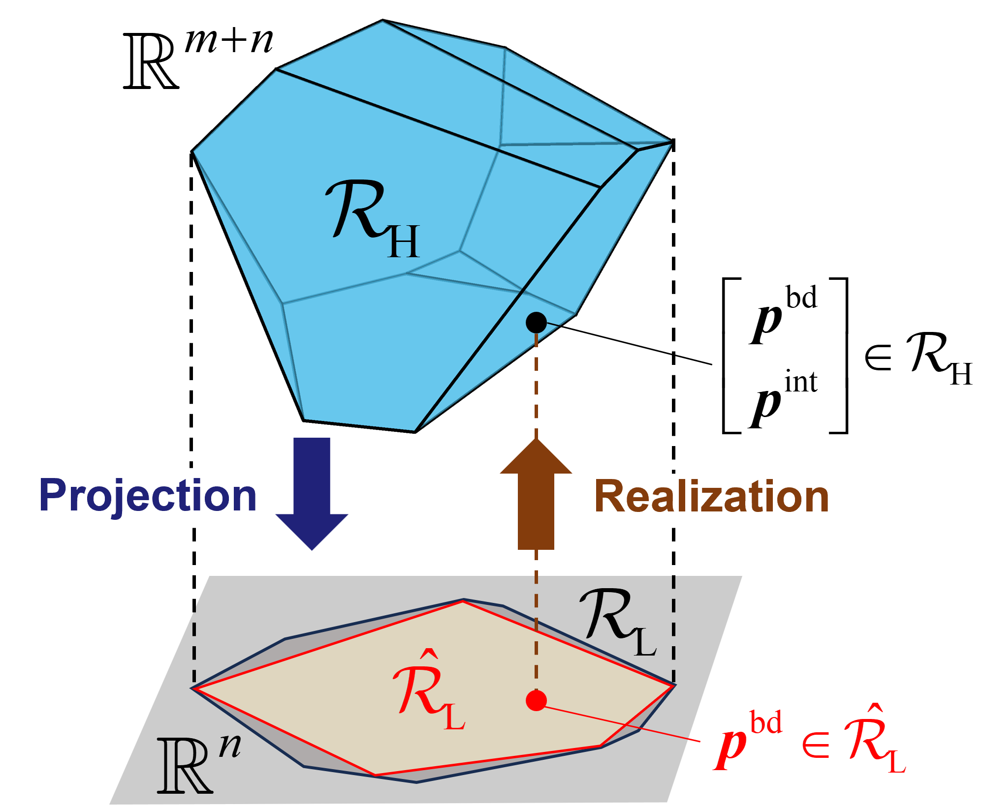
Figure 3: Schematic diagram of the inner-approximate the projected flexibility region.

II-B Overview of Geometric-Based Methods

Using the physical properties and geometric interpretation inherent to flexibility aggregation, shape template-based methods can be used to approximate the flexibility region $\mathcal{R}_{\text{L}}$ [15]. The main physical properties that can be used are the flexibility characteristics of the internal devices. Since the system’s aggregated flexibility is determined by the combination of all devices it contains, if the flexibility regions of these devices share similar shapes, this similarity can be used as a shape template to represent the system’s overall flexibility.

With the linearized approximation [22, 23] of the flexibility regions of devices, they can be expressed in the common linear form:

$$\bm{A}\bm{x}_{i}\leq\bm{b}_{i}$$ (4)

where $\bm{A}$ is a parameter matrix shared by all devices with the same flexibility property, representing the common shape of their flexibility regions. $\bm{x}_{i}$ denotes the decision variables of the $i$-th device, and $\bm{b}_{i}$ refers to the constraint parameters of the $i$-th device. Then, this expression similarity can be used as a shape template for the inner-approximated region as follows:

$$\hat{\mathcal{R}}_{\text{L}}(\bm{b})=\left\{\bm{x}^{\text{bd}}\left\lvert\,\bm{A}\bm{x}^{\text{bd}}\leq\bm{b}\right.\right\},\hat{\mathcal{R}}_{\text{L}}\subset\mathbb{R}^{n}$$ (5)

where $\bm{A}$ is the same matrix as in (4). The vector $\bm{b}$ represents the parameters of the inner-approximated region $\hat{\mathcal{R}}_{\text{L}}$. These parameters need to be adjusted to ensure that the condition $\hat{\mathcal{R}}_{\text{L}}(\bm{b})\subseteq\mathcal{R}_{\text{L}}$ is satisfied. This adjustment can be achieved using our previously developed polytope-bound shrinking algorithm, as detailed in [15, 19].

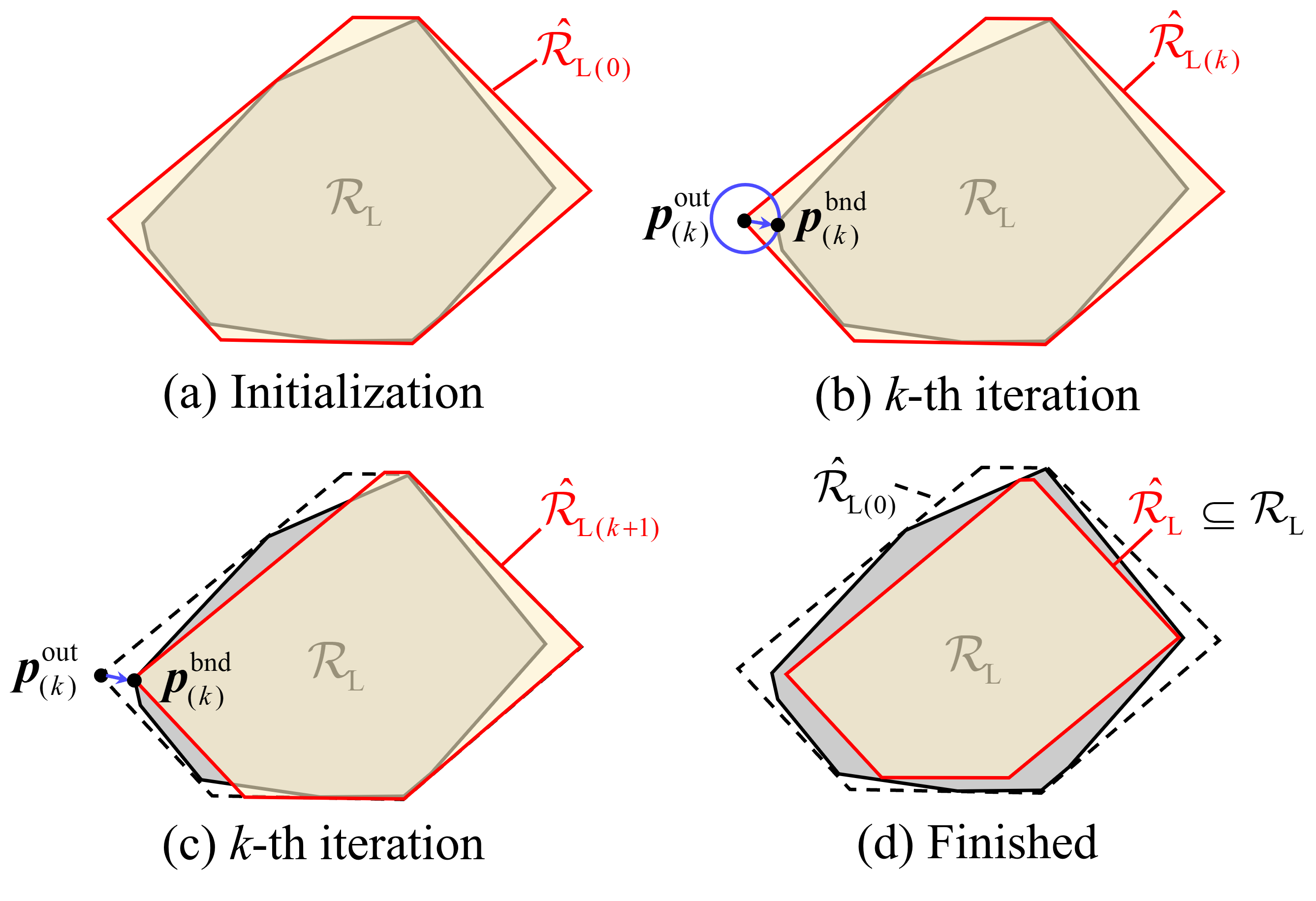
Figure 4: Schematic diagram of the polytope-bound shrinking algorithm: (a) Calculate the circumscribed polytope $\hat{\mathcal{R}}_{\text{L}(0)}$ at the beginning of iteration; (b) Identify the outlier point $\bm{p}^{\text{out}}_{(k)}$ of the shrinking polytope $\hat{\mathcal{R}}_{\text{L}(k)}$ in the current $k$-th iteration. The nearest point on the boundary of the projected polytope $\mathcal{R}_{\text{L}}$ is denoted as $\bm{p}^{\text{bnd}}_{(k)}$; (c) Shrink the boundaries to draw back the extreme point $\bm{p}^{\text{out}}_{(k)}$ to the boundary point $\bm{p}^{\text{bnd}}_{(k)}$ by adjusting parameters $\bm{b}_{(k)}$; (d) Repeat the bound shrinking process to finally obtain the inner-approximated polytope $\hat{\mathcal{R}}_{\text{L}}\subseteq\mathcal{R}_{\text{L}}$.

Fig. 4 is an illustrative diagram that explains the procedure of the algorithm, with the detailed algorithms available in [15]. Inspired by geometric perspective, this algorithm starts from a circumscribed polytope of $\mathcal{R}_{\text{L}}$ with the given template shape and gradually shrinks the boundaries of the inner-approximated region $\hat{\mathcal{R}}_{\text{L}}(\bm{b}_{(k)})$ by gradually adjusting the values of parameters $\bm{b}_{(k)}$ in the $k$-th iteration. Additionally, if all nonzero elements in each row of the matrix $\bm{A}$ in (5) have the same sign, the modified bound-shrinking method [21] can be applied to accelerate calculations.

For the cases where there is no explicit mathematical expression like (5) of the flexibility region—due to complex internal device variables or intricate coupling relationships among boundary variables—the flexibility region can instead be inner-approximated using a high-dimensional ellipsoid shape template [20] as (6).

$$\hat{\mathcal{R}}_{\text{L}}\left(\bm{E},\bm{e}\right)=\left\{\bm{x}^{\text{bd}}\left\lvert\,\left\|\left(\bm{E}\right)^{-1}\left(\bm{x}^{\text{bd}}-\bm{e}\right)\right\|\leq 1\right.\right\}$$ (6)

where $\bm{E}\in\mathbb{R}^{n\times n}$ and $\bm{e}\in\mathbb{R}^{n}$ represent the parameters of the inner-approximated ellipsoid feasible region. The matrix $\bm{E}$ governs the shape of the ellipsoid, and the vector $\bm{e}$ specifies its center. This ellipsoidal shape template can self-adjust to better fit the shape of the projected region with fewer parameters.

To achieve the best possible approximation, the volume of the high-dimensional ellipsoid should be maximized. This process is analogous to inflating an ellipsoid like a balloon within the projected region until it touches the boundaries, reaching its maximum volume.

This problem can be expressed as the following robust optimization problem:

$$\max_{\bm{E}\succeq 0,\bm{e},\bm{x}^{\text{int}}}\left\{\log\operatorname{det}\left(\bm{E}\right)\left\lvert\begin{array}[]{l}\forall\|\bm{\xi}\|\leq 1,\exists\bm{x}^{\text{int}}:\\ \left[\begin{array}[]{c}\bm{E}\bm{\xi}+\bm{e}\\ \bm{x}^{\text{int}}\end{array}\right]\in\mathcal{R}_{\text{H}}\end{array}\right.\right\}$$ (7)

Due to the difficulty in solving the optimization problem (7) in high-dimensional space, the problem can be simplified by introducing specific decision policies between variables $\bm{\xi}$ and $\bm{x}^{\text{int}}$. In engineering applications, adding linear or quadratic policies to the robust problem (7) is a common practice, which allows for an equivalent reformulation as a semi-definite programming (SDP) problem. Details on calculating the parameters $\bm{E}$ and $\bm{e}$ using an equivalent SDP can be found in [20].

III Mathematic Model of a Regional Power Grid

This section introduces the mathematical model of an RPG and the operation constraints that make up the feasible region $\mathcal{R}_{\text{H}}$. The network constraints with the DC power flow model, power balance constraints, $N$-1 security constraints, and generation unit constraints are considered. For clarity in presentation, subscripts indicating the index of the RPG are omitted in this section.

III-A Network and Power Balance Constraints

The operational constraints in a regional power grid are as follows

$$\bm{p}^{\text{inj}}_{t}=\bm{A}^{\text{tpg}}\bm{p}_{t}^{\text{tpg}}+\bm{A}^{\text{rgu}}\bm{p}_{t}^{\text{rgu}}-\bm{A}^{\text{tie}}\bm{p}_{t}^{\text{tie}}-\bm{p}_{t}^{\text{ld}}$$ (8a)

$$-\overline{\bm{p}}^{\text{line}}\leq\bm{S}^{\text{PTDF}}\bm{p}^{\text{inj}}_{t}\leq\overline{\bm{p}}^{\text{line}}$$ (8b)

$$\bm{\theta}_{t}=\theta_{t}^{\text{ref}}+\bm{B}^{-1}\bm{p}^{\text{inj}}_{t},\bm{\theta}_{t}^{\text{bd}}=\bm{M}^{\text{bd}}\bm{\theta}_{t}$$ (8c)

where (8a) calculates the net injection power $\bm{p}^{\text{inj}}_{t}$ of all buses at time $t$. The matrices $\bm{A}^{\text{tpg}}$, $\bm{A}^{\text{rgu}}$, and $\bm{A}^{\text{tie}}$ represent device-bus associations, mapping the indices of each respective device to the corresponding bus indices. (8b) is the transmission line power capability constraints. $\bm{S}^{\text{PTDF}}$ denotes the power transfer distribution factor (PTDF) matrix. The voltage angles of the boundary buses that are directly connected to AC tie-lines, denoted as $\bm{\theta}_{t}^{\text{bd}}$, are calculated in (8c). $\theta_{t}^{\text{ref}}$ denotes the voltage phase angle of the reference node in this RPG relative to the global reference node. $\bm{B}$ denotes the susceptance matrix. $\bm{M}^{\text{bd}}$ is used to select all the indices of boundary buses that directly connected to AC tie-lines

The power balance equation within the RPG is as follows:

$$\bm{1}^{\top}\bm{p}_{t}^{\text{tpg}}+\bm{1}^{\top}\bm{p}_{t}^{\text{rgu}}=\bm{1}^{\top}\bm{p}_{t}^{\text{tie}}+\bm{1}^{\top}\bm{p}_{t}^{\text{ld}}$$ (9)

III-B Generation Units Constraints

The operational constraints for all renewable generation station $i\in\mathcal{I}^{\text{rgu}}$ are as follows

$$\underline{p}^{\text{rgu}}_{i}\leq p_{i,t}^{\text{rgu}}\leq\overline{p}^{\text{fore}}_{i,t}$$ (10)

where $\overline{p}^{\text{fore}}_{i,t}$ denotes the maximum predicted output power of the $i$-th renewable generation station at time $t$.

Furthermore, the operational constraints for all thermal power generators $i\in\mathcal{I}^{\text{tpg}}$ are as follows:

$$\underline{p}^{\text{tpg}}_{i}+Rd^{\text{tpg}}_{i,t}\leq p_{i,t}^{\text{tpg}}\leq\overline{p}^{\text{tpg}}_{i}-Ru^{\text{tpg}}_{i,t}$$ (11a)

$$\underline{r}^{\text{tpg}}_{i,t}\leq\left(p_{i,t+1}^{\text{tpg}}-p_{i,t}^{\text{tpg}}\right)/{\Delta t}\leq\overline{r}^{\text{tpg}}_{i,t}$$ (11b)

$$0\leq Rd^{\text{tpg}}_{i,t}\leq\overline{Rd}^{\text{tpg}}_{i,t},0\leq Ru^{\text{tpg}}_{i,t}\leq\overline{Ru}^{\text{tpg}}_{i,t}$$ (11c)

$$\sum\limits_{i\in\mathcal{I}^{\text{tpg}}}Rd^{\text{tpg}}_{i,t}\geq Rd^{\text{req}}_{t},\sum\limits_{i\in\mathcal{I}^{\text{tpg}}}Ru^{\text{tpg}}_{i,t}\geq Ru^{\text{req}}_{t}$$ (11d)

where (11a) and (11b) are the power and ramp rate constraints, respectively. (11c) and (11d) are the reserve constraints. $Rd^{\text{req}}_{t}$ and $Ru^{\text{req}}_{t}$ denote the total down and up reserve requirements of the entire RPG at time $t$, as determined by the dispatch center based on the fluctuation in the generation of renewable energy and load power [24].

III-C N-1 Security Constraints

To safeguard the power grid when a fault occurs in critical equipment, such as transmission lines and generators, the $N$-1 security constraints are considered in the security constants of RPG. For $\forall c\in\mathcal{C}$:

$$\bm{p}^{\text{inj}}_{t,c}=\bm{A}^{\text{tpg}}\bm{p}_{t,c}^{\text{tpg}}+\bm{A}^{\text{rgu}}\bm{p}_{t,c}^{\text{rgu}}-\bm{A}^{\text{tie}}\bm{p}_{t}^{\text{tie}}-\bm{p}_{t}^{\text{ld}}$$ (12a)

$$-\overline{\bm{p}}^{\text{line}}\leq\bm{S}^{\text{PTDF}}\bm{p}^{\text{inj}}_{t,c}\leq\overline{\bm{p}}^{\text{line}}$$ (12b)

$$\bm{1}^{\top}\bm{p}_{t,c}^{\text{tpg}}+\bm{1}^{\top}\bm{p}_{t,c}^{\text{rgu}}=\bm{1}^{\top}\bm{p}_{t}^{\text{tie}}+\bm{1}^{\top}\bm{p}_{t}^{\text{ld}}$$ (12c)

$$\underline{\bm{p}}^{\text{tpg}}\leq\bm{p}_{t,c}^{\text{tpg}}\leq\overline{\bm{p}}^{\text{tpg}},\underline{\bm{p}}^{\text{rgu}}\leq\bm{p}_{t,c}^{\text{rgu}}\leq\overline{\bm{p}}^{\text{fore}}_{t}$$ (12d)

$$\left|\bm{p}_{t,c}^{\text{tpg}}-\bm{p}_{t}^{\text{tpg}}\right|\leq\Delta\bm{p}^{\text{tpg}},\left|\bm{p}_{t,c}^{\text{rgu}}-\bm{p}_{t}^{\text{rgu}}\right|\leq\Delta\bm{p}^{\text{rgu}}$$ (12e)

$$\bm{\theta}_{t,c}=\theta_{t}^{\text{ref}}+\bm{B}^{-1}_{c}\bm{p}^{\text{inj}}_{t,c},\left|\bm{\theta}_{t,c}-\bm{\theta}_{t}\right|\leq\Delta\bm{\theta}$$ (12f)

where the subscript $c$ represents the index of $N$-1 contingency scenarios, and $\mathcal{C}$ is the index set of key contingency. $\Delta\bm{p}^{\text{tpg}}$, $\Delta\bm{p}^{\text{rgu}}$ and $\Delta\bm{\theta}$ denote the maximum allowable variations of the power output of thermal power generators and renewable generation stations, as well as the voltage angles of buses in the contingency scenarios, respectively.

III-D Stochastic Factors Consideration

The forecasts for the load and renewable energy generation contain inherent random errors, which introduce stochastic factors into the RPGs model. Using historical data, existing methods can convert the constraints with stochastic variables into deterministic constraints. For example, the Gaussian Mixture Model (GMM) approximates the probability distribution of stochastic variables, enabling the conversion of constraints into deterministic equivalents through the chance constraint method at a specified confidence level [24, 23]. Moreover, distributionally robust optimization converts joint chance constraints into deterministic constraints by considering the distance between the potential variable distributions and the empirical distribution [25]. Using either approach, the stochastic RPG model can be effectively transformed into a deterministic model, which serves as the model basis for computing the aggregated RPG model proposed in this work.

III-E Model Integration

By integrating all the operational constraints of RPG (8)-(12), the feasible operation region of the RPG can be defined in a high-dimensional polytopal form as follows:

$$\mathcal{R}_{\text{H}}=\left\{\left[\begin{array}[]{l}\bm{x}^{\text{bd}}\\ \bm{x}^{\text{int}}\end{array}\right]\left\lvert\,\begin{array}[]{l}\bm{x}^{\text{bd}}=\bm{C}\bm{x}^{\text{int}}+\bm{d}\\ \bm{F}\bm{x}^{\text{int}}\leq\bm{f}\end{array}\right.\right\}$$ (13)

where the matrices $\bm{C}$, $\bm{D}$, $\bm{F}$, vectors $\bm{d}$ and $\bm{f}$ are constant parameters that can be obtained by integrating constraints (8)-(12). $\bm{x}^{\text{int}}$ and $\bm{x}^{\text{bd}}$ are internal and boundary variables, defined as follows.

The internal variables $\bm{x}^{\text{int}}$ include all the variables of power generation units, and network states, under both normal and $N$-1 contingency operation conditions.

The boundary variables $\bm{x}^{\text{bd}}$ include the output power of the tie-lines $\bm{p}^{\text{tie}}_{t}$, and the voltage angles of the boundary buses connected directly to the AC tie-lines $\bm{\theta}^{\text{bd}}_{t}$, as follows:

$$\bm{x}^{\text{bd}}:=\underset{t\in\mathcal{T}}{\operatorname{col}}(\bm{x}^{\text{bd}}_{t}),\bm{x}^{\text{bd}}_{t}:=\left[\left(\bm{p}^{\text{tie}}_{t}\right)^{\top}\left(\bm{\theta}^{\text{bd}}_{t}\right)^{\top}\right]^{\top}$$ (14)

This choice of boundary variables is based on the fact that the transmission power of the DC tie-lines is directly controlled by converters, whereas the AC tie-line power transmission depends on the voltage angles of the boundary buses [3], governed by power balance and network constraints

$$p_{r,ij,t}^{\text{tie}}=-p_{s,ji,t}^{\text{tie}}=\left(\theta_{r,i,t}^{\text{bd}}-\theta_{s,j,t}^{\text{bd}}\right)/{x_{ij}}$$ (15)

where $\theta_{r,i,t}^{\text{bd}}$ and $\theta_{s,j,t}^{\text{bd}}$ denote the voltage angles of the $i$-th bus in region $r$ and the $j$-th bus in region $s$ at time $t$, respectively. $p_{r,ij,t}^{\text{tie}}$ and $p_{s,ji,t}^{\text{tie}}$ represent power flows from region $r$ to region $s$ through tie-line $ij$ and vice versa, respectively, and $x_{ij}$ is the reactance of this AC tie-line $ij$.

Subsequently, the flexibility aggregation problem of an RPG can be converted to the projection problem of the high-dimensional feasibility region $\mathcal{R}_{\text{H}}$ onto the lower-dimensional region $\mathcal{R}_{\text{L}}\subset\operatorname{space}(\bm{x}^{\text{bd}})$.

IV Aggregated Model Calculation for A Regional Power Grid

IV-A Dimension-Decomposition-Based Calculation of Aggregated Flexibility Region

This section presents the proposed dimension-decomposition-based method for calculating the aggregated flexibility region of an RPG. The process consists of five key steps: 1) Analyze the temporal and spatial coupling relationships of boundary variables; 2) Decompose the flexibility region into a series of lower-dimensional subspaces using dimensionality reduction projection; 3) Approximate the projected regions within these subspaces using different shape templates; 4) Reconstruct the overall inner-approximated flexibility region in $\operatorname{space}(\bm{x}^{\text{bd}})$ by recombining the inner-approximated regions in the subspaces; and 5) Adjust the parameters to ensure that the inner approximation condition $\hat{\mathcal{R}}_{\text{L}}\subseteq\mathcal{R}_{\text{L}}$ is satisfied. A detailed explanation of each step follows, with an illustrative diagram provided in Fig. 6.

IV-A1 Analysis of Boundary Variables

To calculate the aggregated flexibility region $\mathcal{R}_{\text{L}}$ of an RPG in $\operatorname{space}(\bm{x}^{\text{bd}})$, it is crucial to understand the coupling relationships between the boundary variables $\bm{x}^{\text{bd}}$ first. By analyzing the coupling constraints of the boundary variables in (8)-(12), all the constraints can be categorized into two types. Accordingly, all the boundary variables can be categorized into two groups of variable sets, as illustrated in Fig. 5.

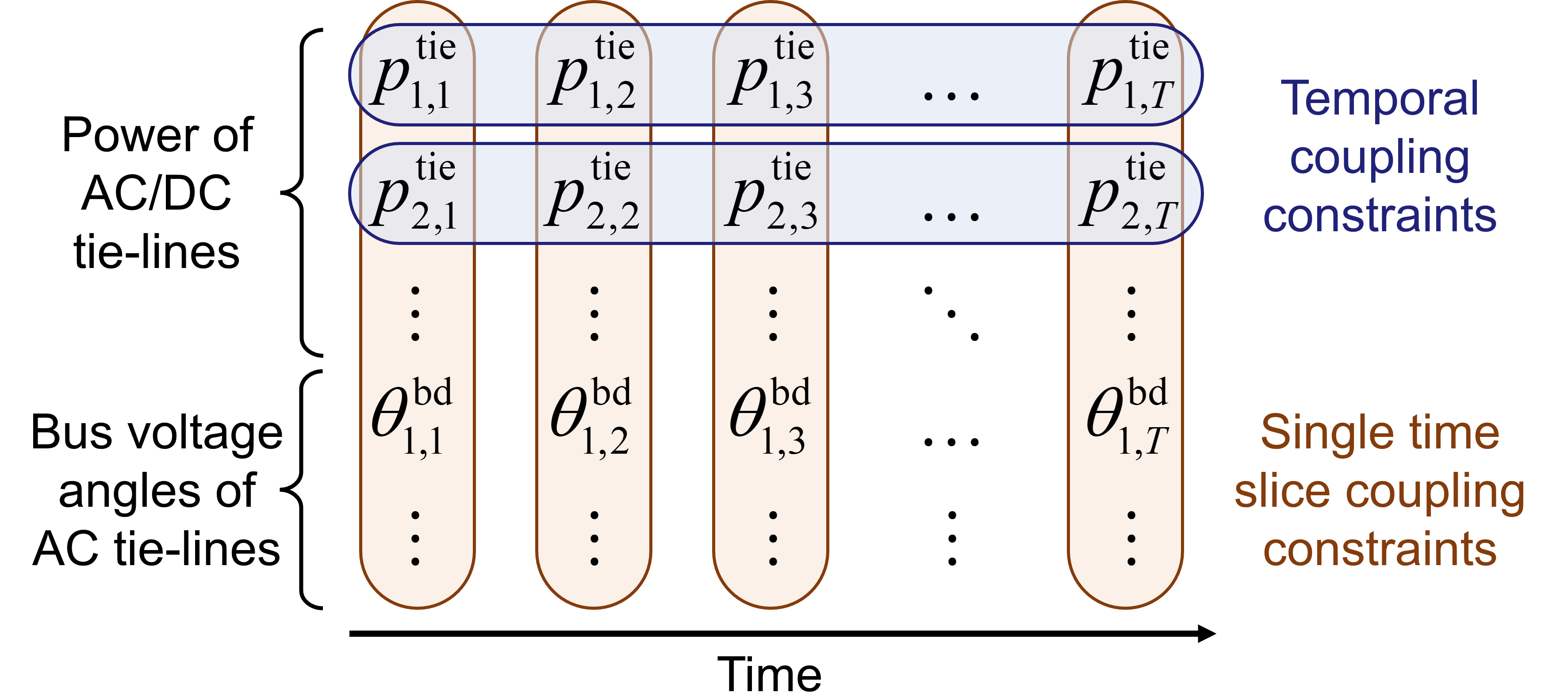
Figure 5: The coupling constraints of boundary variables for a regional power grid.

The first category, temporal coupling constraints, addresses the active output power constraints across all time slots for a single tie-line, denoted as

$$\bm{p}^{\text{tie}}_{i}:=\underset{t\in\mathcal{T}}{\operatorname{col}}(\bm{p}^{\text{tie}}_{i,t}):=\bm{S}^{\text{bd}}_{i}\bm{x}^{\text{bd}},\forall i\in\mathcal{I}^{\text{tie}}$$ (16)

This form of coupling is mainly driven by generator operation constraints (11) and power balance constraints (9). Consequently, the active output power across time slots for a single tie-line exhibits temporal coupling characteristics, similar to those observed in thermal power generators, which are regulated by both power and ramp rate constraints.

The second category, single time slice coupling constraints, encompasses coupling constraints for boundary variables within each individual time slice $t$, denoted as

$$\bm{x}^{\text{bd}}_{t}:=\bm{H}^{\text{bd}}_{t}\bm{x}^{\text{bd}},\forall t\in\mathcal{T}$$ (17)

These relationships are governed by constraints that apply independently within each time slice, such as network constants (8b), power balance (9), and $N$-1 security constraints (12).

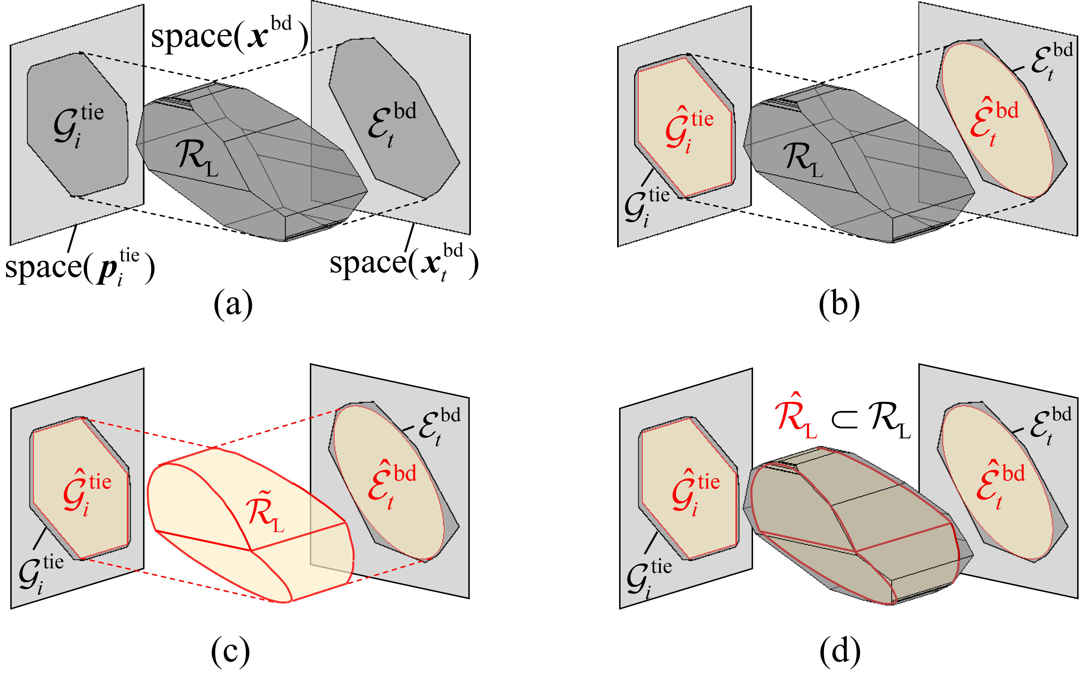
Figure 6: Dimension decomposition and recombination process of the aggregated flexibility region: (a) Project the aggregated flexibility region $\mathcal{R}_{\text{L}}$ onto two groups of lower-dimensional subspaces; (b) Inner-approximate the polytopes in the subspaces with appropriate shape templates; (c) Recombine the inner-approximated polytopes from subspaces to obtain the aggregated flexibility region $\tilde{\mathcal{R}}_{\text{L}}$ in $\operatorname{space}(\bm{x}^{\text{bd}})$; (d) Adjust the parameters to obtain the inner-approximated aggregated flexibility region $\hat{\mathcal{R}}_{\text{L}}\subseteq\mathcal{R}_{\text{L}}$.

IV-A2 Dimension Decomposition

The coupling relationships of the boundary variables in an RPG can be divided into two categories. Accordingly, the aggregated flexibility region $\mathcal{R}_{\text{L}}\subset\operatorname{space}(\bm{x}^{\text{bd}})$ can, from a geometric perspective, be decomposed into two corresponding groups of subspaces: $\operatorname{space}(\bm{x}^{\text{bd}}_{t})$ for $t\in\mathcal{T}$, and $\operatorname{space}(\bm{p}^{\text{tie}}_{i})$ for $i\in\mathcal{I}^{\text{tie}}$.

To express the coupling relationships within these subspaces, the aggregated flexibility region $\mathcal{R}_{\text{L}}$ can be projected onto lower-dimensional subspaces. Denote the projected polytopes as $\mathcal{E}^{\text{bd}}_{t}\subset\operatorname{space}(\bm{x}^{\text{bd}}_{t})$ for $t\in\mathcal{T}$, and $\mathcal{G}^{\text{tie}}_{i}\subset\operatorname{space}(\bm{p}^{\text{tie}}_{i})$ for $i\in\mathcal{I}^{\text{tie}}$, respectively. An illustrated diagram is shown in Fig. 6(a).

IV-A3 Inner Approximation of Projected Polytopes in the Subspaces

To explicitly calculate the expression of coupling constraints in each subspace, the polytopes $\mathcal{E}^{\text{bd}}_{t}$ and $\mathcal{G}^{\text{tie}}_{i}$ are inner-approximated, respectively, as shown in Fig. 6(b).

Since the temporal coupling constraints for a single tie-lie exhibit generator-like temporal coupling characteristics, the polytopes $\mathcal{G}^{\text{tie}}_{i}$ can be inner-approximated by the generator-like polytopal shape templates, denoted as $\hat{\mathcal{G}}^{\text{tie}}_{i}$.

$$\hat{\mathcal{G}}^{\text{tie}}_{i}\left(\bm{b}^{\text{tie}}_{i}\right):=\left\{\bm{p}^{\text{tie}}_{i}\left\lvert\,\begin{array}[]{c}\underline{r}^{\text{tie}}_{i,t}\leq(p^{\text{tie}}_{i,t+1}-p^{\text{tie}}_{i,t})/{\Delta t}\leq\overline{r}^{\text{tie}}_{i,t},\\ \underline{p}^{\text{tie}}_{i,t}\leq p^{\text{tie}}_{i,t}\leq\overline{p}^{\text{tie}}_{i,t},\forall t\in\mathcal{T}\end{array}\right.\right\}$$ (18)

where the vector $\bm{b}^{\text{tie}}_{i}$ collects all the parameters of the generator-like polytope shape template, defined as follows:

$$\bm{b}^{\text{tie}}_{i}:=\\ \left[(\overline{\bm{p}}^{\text{tie}}_{i})^{\top}-(\underline{\bm{p}}^{\text{tie}}_{i})^{\top}(\overline{\bm{r}}^{\text{tie}}_{i})^{\top}-(\underline{\bm{r}}^{\text{tie}}_{i})^{\top}\right]^{\top}$$ (19)

where $\overline{\bm{p}}^{\text{tie}}_{i}:=\operatorname{col}_{t}(\overline{p}^{\text{tie}}_{i,t})$, $\underline{\bm{p}}^{\text{tie}}_{i}:=\operatorname{col}_{t}(\underline{p}^{\text{tie}}_{i,t})$, $\overline{\bm{r}}^{\text{tie}}_{i}:=\operatorname{col}_{t}(\overline{r}^{\text{tie}}_{i,t})$, $\underline{\bm{r}}^{\text{tie}}_{i}:=\operatorname{col}_{t}(\underline{r}^{\text{tie}}_{i,t})$. $\bm{b}^{\text{tie}}_{i}$ can be calculated based on the bound shrinking algorithm [15] introduced in Section II-B. Then, (18) can be rewritten as the following compact matrix form:

$$\hat{\mathcal{G}}^{\text{tie}}_{i}\left(\bm{b}^{\text{tie}}_{i}\right)=\left\{\bm{p}^{\text{tie}}_{i}\left\lvert\,\bm{A}^{\text{tie}}_{i}\bm{p}^{\text{tie}}_{i}\leq\bm{b}^{\text{tie}}_{i}\right.\right\}$$ (20)

The single time slice coupling constraints are governed by the complex coupling relationships among the coupling variables that lack an explicit expression, the polytopes $\mathcal{E}^{\text{bd}}_{t}$ can be inner-approximated by the ellipsoidal shape templates, denoted as $\hat{\mathcal{E}}^{\text{bd}}_{t}$.

$$\hat{\mathcal{E}}_{t}^{\text{bd}}\left(\bm{E}_{t}^{\text{bd}},\bm{e}_{t}^{\text{bd}}\right):=\left\{\bm{x}_{t}^{\text{bd}}\left\lvert\,\left\|\left(\bm{E}_{t}^{\text{bd}}\right)^{-1}\left(\bm{x}_{t}^{\text{bd}}-\bm{e}_{t}^{\text{bd}}\right)\right\|\leq 1\right.\right\}$$ (21)

The parameters $\bm{E}_{t}^{\text{bd}}$ and $\bm{e}_{t}^{\text{bd}}$ can be calculated based on the methods introduced in Section II-B.

Notably, the independence of projection and inner approximation calculations in each subspace allows the computation of parameters—$\bm{b}^{\text{tie}}_{i}$ for $i\in\mathcal{I}^{\text{tie}}$, as well as $\bm{E}_{t}^{\text{bd}}$ and $\bm{e}_{t}^{\text{bd}}$ for $t\in\mathcal{T}$—to be efficiently accelerated through parallel computing.

IV-A4 Dimension Recombination

As demonstrated in Fig. 6(c), to form the overall flexibility region, the inner-approximated regions $\mathcal{E}^{\text{bd}}_{t}$ for $t\in\mathcal{T}$, and $\mathcal{G}^{\text{tie}}_{i}$ for $i\in\mathcal{I}^{\text{tie}}$ are recombined in $\operatorname{space}(\bm{x}^{\text{bd}})$ as follows:

$$\tilde{\mathcal{R}}_{\text{L}}:=\left\{\bm{x}^{\text{bd}}\left\lvert\,\begin{array}[]{c}\bm{S}^{\text{tie}}_{i}\bm{x}^{\text{bd}}\in\hat{\mathcal{G}}^{\text{tie}}_{i}\left(\tilde{\bm{b}}^{\text{tie}}_{i}\right),\forall i\in\mathcal{I}^{\text{tie}}\\ \bm{H}^{\text{bd}}_{t}\bm{x}^{\text{bd}}\in\hat{\mathcal{E}}_{t}^{\text{bd}}\left(\tilde{\bm{E}}_{t}^{\text{bd}},\bm{e}_{t}^{\text{bd}}\right),\forall t\in\mathcal{T}\end{array}\right.\right\}$$ (22)

where the constant matrices $\bm{S}^{\text{tie}}_{i}$ and $\bm{H}^{\text{bd}}_{t}$ are used to select the elements $\bm{p}^{\text{tie}}_{i}$ and $\bm{x}^{\text{bd}}_{t}$ from all the boundary variables $\bm{x}^{\text{bd}}$ as defined in (16) and (17), respectively. The recombination region is an approximation of $\mathcal{R}_{\text{L}}$, denoted as $\tilde{\mathcal{R}}_{\text{L}}$, where the parameters $\tilde{\bm{b}}^{\text{tie}}_{i}$ and $\tilde{\bm{E}}_{t}^{\text{bd}}$ still need further adjustments in the following step.

IV-A5 Parameters Adjustments

To finally obtain the inner-approximated $\hat{\mathcal{R}}_{\text{L}}\subseteq\mathcal{R}_{\text{L}}$, further adjustments are required to the parameters of $\tilde{\mathcal{R}}_{\text{L}}$. The parameters adjustment can be achieved iteratively by shrinking the bounds of $\hat{\mathcal{G}}^{\text{tie}}_{i}(\tilde{\bm{b}}^{\text{tie}}_{i})$ and $\hat{\mathcal{E}}_{t}^{\text{bd}}(\tilde{\bm{E}}_{t}^{\text{bd}},\bm{e}_{t}^{\text{bd}})$ that make up $\tilde{\mathcal{R}}_{\text{L}}$. In each iteration, the parameters are updated to shrink the flexibility region. Denote the parameters in the $k$-th iteration as $\bm{b}^{\text{tie}}_{i(k)}$ and $\bm{E}_{t(k)}^{\text{bd}}$, and the flexibility region in the $k$-th iteration as $\hat{\mathcal{R}}_{\text{L}(k)}$. The iteration stops until the condition $\hat{\mathcal{R}}_{\text{L}(k)}\subseteq\mathcal{R}_{\text{L}}$ is met. The initial values of the parameters in the iteration can be obtained in the previous dimension recombination step, denoted as $\bm{b}^{\text{tie}}_{i(0)}:=\tilde{\bm{b}}^{\text{tie}}_{i}$ and $\bm{E}_{t(0)}^{\text{bd}}:=\tilde{\bm{E}}_{t}^{\text{bd}}$.

At the beginning of each iteration, the potential outliers, denoted as $\bm{x}^{\text{out}}_{(k)}$, such that $\bm{x}^{\text{out}}_{(k)}\in\hat{\mathcal{R}}_{\text{L}(k)}$ but $\bm{x}^{\text{out}}_{(k)}\notin\mathcal{R}_{\text{L}}$, are identified by solving a Stackelberg game [12, 15] as follows:

$$\min_{\bm{x}^{\text{bd}}}\max_{\bm{x}^{\text{int}}}0$$ (23a)

s.t. $$\bm{H}_{t}^{\text{bd}}\bm{x}^{\text{bd}}\in\hat{\mathcal{E}}_{t}^{\text{bd}}\left(\bm{E}_{t(k)}^{\text{bd}},\bm{e}_{t}^{\text{bd}}\right),\forall t\in\mathcal{T}$$ (23b)

$$\bm{A}^{\text{tie}}_{i}\bm{S}^{\text{tie}}_{i}\bm{x}^{\text{bd}}\leq\bm{b}^{\text{tie}}_{i(k)},\forall i\in\mathcal{I}^{\text{tie}}$$ (23c)

$$\bm{x}^{\text{bd}}=\bm{C}\bm{x}^{\text{int}}+\bm{d}$$ (23d)

$$\bm{F}\bm{x}^{\text{int}}\leq\bm{f}$$ (23e)

In this Stackelberg game, the leader variables, $\bm{x}^{\text{bd}}$, aims to guarantee the feasibility of the problem, while the follower variables, $\bm{x}^{\text{int}}$, seeks to make it infeasible. If the follower’s maximization problem is infeasible, it indicates the existence of an outlier $\bm{x}^{\text{out}}_{(k)}$, such that $\bm{x}^{\text{out}}_{(k)}\in\hat{\mathcal{R}}_{\text{L}(k)}$ but $\bm{x}^{\text{out}}_{(k)}\notin\mathcal{R}_{\text{L}}$. In this case, the optimal objective value of (23) is $-\infty$. Otherwise, if the follower’s maximization problem is feasible, no such outlier exists, confirming that $\hat{\mathcal{R}}_{\text{L}(k)}\subseteq\mathcal{R}_{\text{L}}$, and the optimal objective value is 0. The problem (23) can be converted into an MILP formulation and solved, as described in detail in the supplemental file [26].

If an outlier $\bm{x}^{\text{out}}_{(k)}$ is located by solving (23), the nearest point on the boundary of $\mathcal{R}_{\text{L}}$, denoted as $\bm{x}^{\text{bnd}}_{(k)}\in\partial\mathcal{R}_{\text{L}}$, can be obtained by solving the following optimization problem:

$$\bm{x}^{\text{bnd}}_{(k)} =\underset{\bm{x}^{\text{bd}}}{\operatorname{argmin}}\left\|\bm{x}^{\text{out}}_{(k)}-\bm{x}^{\text{bd}}\right\|$$ (24a)

s.t. $$\left[(\bm{x}^{\text{bd}})^{\top}(\bm{x}^{\text{int}})^{\top}\right]^{\top}\in\mathcal{R}_{\text{H}}$$ (24b)

After identifying the outlier $\bm{x}^{\text{out}}_{(k)}$ and the nearest boundary point $\bm{x}^{\text{bnd}}_{(k)}$, the parameters are modified to shrink the related bounds of $\hat{\mathcal{R}}_{\text{L}(k)}$ to draw back the outlier $\bm{x}^{\text{out}}_{(k)}$ to $\bm{x}^{\text{bnd}}_{(k)}$, as shown in Fig. 4(c). The index set of related bounds that $\bm{x}^{\text{out}}_{(k)}\in\partial\hat{\mathcal{R}}_{\text{L}(k)}$ can be identified as follows:

$$\mathcal{T}_{(k)}:=\left\{t\in\mathcal{T}\left\lvert\bm{H}^{\text{bd}}_{t}\bm{x}^{\text{out}}_{(k)}\in\partial\hat{\mathcal{E}}_{t}^{\text{bd}}(\bm{E}_{t(k)}^{\text{bd}},\bm{e}_{t}^{\text{bd}})\right.\right\}$$ (25a)

$$\mathcal{I}^{\text{tie}}_{(k)}:=\left\{i\in\mathcal{I}^{\text{tie}}\left\lvert\bm{S}^{\text{tie}}_{i}\bm{x}^{\text{out}}_{(k)}\in\partial\hat{\mathcal{G}}^{\text{tie}}_{i}(\bm{b}^{\text{tie}}_{i(k)})\right.\right\}$$ (25b)

$$\mathcal{J}_{i(k)}:=\left\{j\left\lvert(\bm{A}^{\text{tie}}_{i})_{j}\bm{S}^{\text{tie}}_{i}\bm{x}^{\text{out}}_{(k)}=(\bm{b}^{\text{tie}}_{i(k)})_{j}\right.\right\},\forall i\in\mathcal{I}^{\text{tie}}_{(k)}$$ (25c)

Subsequently, the bounds of $\hat{\mathcal{R}}_{\text{L}(k)}$ are shrunk by adjusting the parameters $\bm{E}_{t(k)}^{\text{bd}}$ and $\bm{b}^{\text{tie}}_{i(k)}$.

For regions inner-approximated with an ellipsoidal shape template, the radius is shrunk by scaling the shape matrix $\bm{E}_{t(k)}^{\text{bd}}$ with a factor $\rho_{t}$, while the center point vector $\bm{e}_{t}^{\text{bd}}$ remains fixed, $\forall t\in\mathcal{T}_{(k)}$:

$$\bm{E}_{t(k+1)}^{\text{bd}}=\rho_{t}\bm{E}_{t(k)}^{\text{bd}},$$ (26a)

$$\rho_{t}:=\left\|(\bm{E}_{t(k)}^{\text{bd}})^{-1}(\bm{H}^{\text{bd}}_{t}\bm{x}^{\text{bnd}}_{(k)}-\bm{e}_{t}^{\text{bd}})\right\|$$ (26b)

For regions inner-approximated with a polytopal shape template, the bounds are shrunk by adjusting the right-hand side parameters, $\bm{b}^{\text{tie}}_{i(k)}$, $\forall i\in\mathcal{I}^{\text{tie}}_{(k)}$:

$$(\bm{b}^{\text{tie}}_{i(k+1)})_{j}=\left\{\begin{array}[]{l}(\bm{A}^{\text{tie}}_{i})_{j}\bm{S}^{\text{tie}}_{i}\bm{x}^{\text{bnd}}_{(k)},\text{if}\>j\in\mathcal{J}_{i(k)}\\ (\bm{b}^{\text{tie}}_{i(k)})_{j},\text{if}\>j\notin\mathcal{J}_{i(k)}\end{array}\right.$$ (27)

Then update $k\leftarrow k+1$ and proceed to solve (23) to check for the existence of outliers in $\hat{\mathcal{R}}_{\text{L}(k+1)}$.

The pseudocode of the dimension-decomposition-based bound shrinking algorithm used to adjust the parameters is summarized in Algorithm 1.

Algorithm 1 Dimension-Decomposition-Based Bound Shrinking Algorithm

1: Initialize bound shrinking using the parameters obtained from dimension decomposition and set $k=0$.

2: Solve (23) to check for the existence of an outlier $\bm{x}^{\text{out}}_{(k)}\in\hat{\mathcal{R}}_{\text{L}(k)}$ but $\bm{x}^{\text{out}}_{(k)}\notin\mathcal{R}_{\text{L}}$. If the optimal objective value of (23) is 0, exit the algorithm and output $\hat{\mathcal{R}}_{\text{L}(k)}$ as the final result; otherwise, proceed to Step 3.

3: Solve (24) to find the nearest point $\bm{x}^{\text{bnd}}_{(k)}\in\partial\mathcal{R}_{\text{L}}$.

4: Solve (25) to select the indices of the bounds of $\hat{\mathcal{R}}_{\text{L}(k)}$ that $\bm{x}^{\text{out}}_{(k)}$ resides.

5: Shrink the related bounds of $\hat{\mathcal{R}}_{\text{L}(k)}$ by adjusting the parameters as in (26) and (27).

6: Update $k\leftarrow k+1$ and return to Step 2.

Finally, the aggregated flexibility region of RPG is obtained as follows:

$$\hat{\mathcal{R}}_{\text{L}}:=\left\{\bm{x}^{\text{bd}}\left\lvert\,\begin{array}[]{c}\bm{A}^{\text{tie}}_{i}\bm{S}^{\text{tie}}_{i}\bm{x}^{\text{bd}}\leq\bm{b}^{\text{tie}}_{i},\forall i\in\mathcal{I}^{\text{tie}}\\ \left\|\left(\bm{E}_{t}^{\text{bd}}\right)^{-1}\left(\bm{H}^{\text{bd}}_{t}\bm{x}^{\text{bd}}-\bm{e}_{t}^{\text{bd}}\right)\right\|\leq 1,\forall t\in\mathcal{T}\end{array}\right.\right\}$$ (28)

IV-B Physical Counterpart of the Flexibility Aggregation Model

The flexibility aggregation model derived through geometric projection calculations can be interpreted in terms of physical significance, as the parameters of the aggregated flexibility region of the RPG have a clear physical meaning.

For a single tie-line, its flexibility region across all time slots can be represented by an equivalent generator model, constrained by both power and ramp rate constraints, corresponding to the temporal coupling constraints in (18).

For a single time slice, the output power and bus voltage angles of all equivalent generators are interconnected through the constraints in the ellipsoidal expression form, corresponding to the single time slice coupling constraints in (21).

Therefore, after flexibility aggregation, the entire RPG can be equivalent to a group of generators that interconnected through coupling constraints, as shown in the schematic diagram Fig. 7.

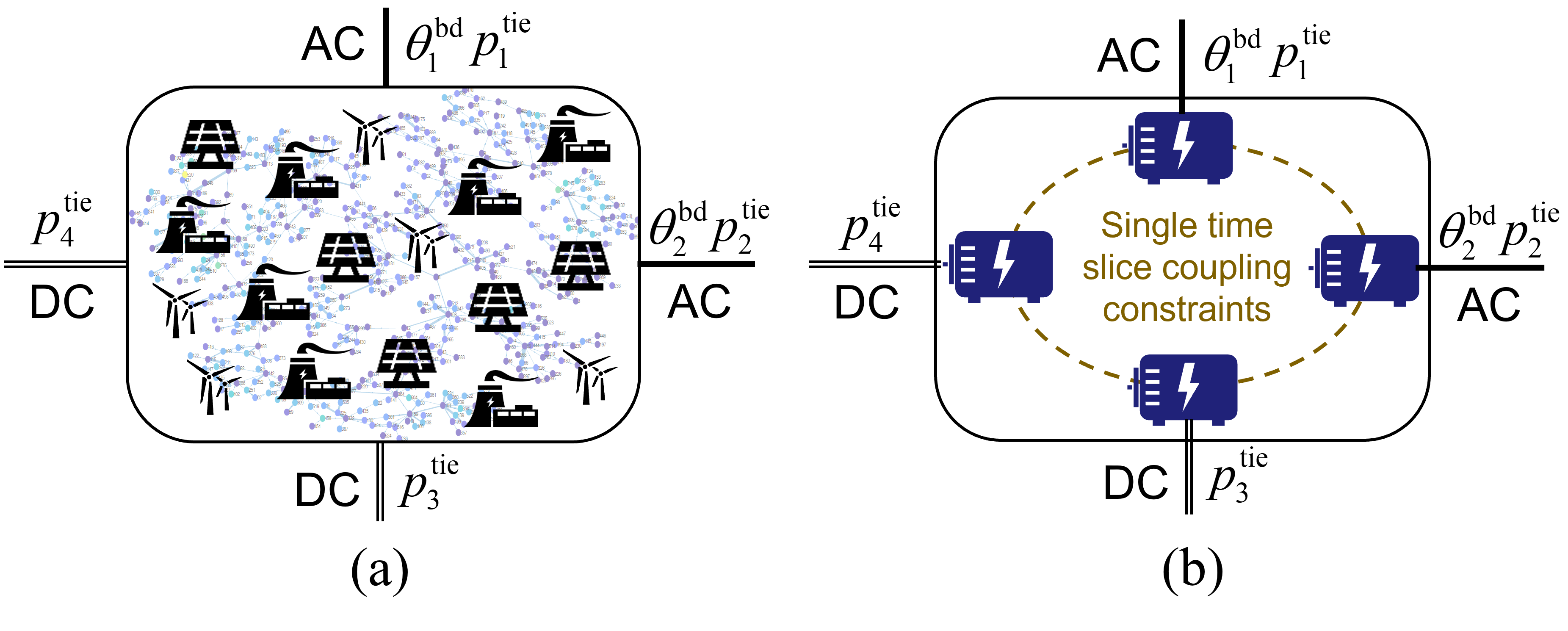
Figure 7: (a) The original regional power grid; (b) Physical counterpart: equivalent generators model via flexibility aggregation.

IV-C Aggregated Operational Cost Function

To facilitate coordinated economic dispatch of interconnected RPGs, the analytical aggregated cost function of RPG is derived with the piecewise linear fitting [27]. The total operational cost of an RPG is the sum of the operational costs of each generation unit. From an external system perspective, the operational cost of an RPG, denoted as $\kappa_{t}$, is a function of the power flow through all tie-lines, denoted as $\bm{p}^{\text{tie}}_{t}$. To model this aggregated cost function, uniform sampling is applied across each dimension of the feasible domain, yielding a total of $J$ samples of tie-line power flows and their corresponding operational costs. The operating point and the corresponding cost of the $j$-th sample are denoted by $\bm{p}^{\text{tie}}_{t(j)}$ and $\kappa_{t(j)}$, respectively. By solving the following optimal power flow problem, the minimum operational cost $\kappa_{t(j)}$ for the $j$-th operating point $\bm{p}^{\text{tie}}_{t(j)}$ can be obtained:

$$\kappa_{t(j)}= \underset{\bm{p}^{\text{tpg}}_{t}}{\operatorname{min}}\sum_{i\in\mathcal{I}^{\text{tpg}}}\left(\begin{array}[]{l}a^{\text{tpg}}_{i}(p^{\text{tpg}}_{i,t})^{2}+b^{\text{tpg}}_{i}p^{\text{tpg}}_{i,t}+c^{\text{tpg}}_{i}\\ +d^{\text{tpg}}_{i}Ru^{\text{tpg}}_{i,t}+e^{\text{tpg}}_{i}Rd^{\text{tpg}}_{i,t}\end{array}\right)$$ (29c)

s.t. $$\bm{p}^{\text{tie}}_{t}=\bm{p}^{\text{tie}}_{t(j)}$$ (29d)

$$\text{Constraints}\,\eqref{eq-RPGCons}-\eqref{eq-RPGN1Cons}$$

where $a^{\text{tpg}}_{i}\sim e^{\text{tpg}}_{i}$ are the cost coefficients of the $i$-th thermal power generators in the RPG.

Subsequently, the convex piecewise linear fitting algorithm [28] is applied to fit these $J$ sample points into an analytical expression representing the aggregated operational cost function, denoted as

$$\kappa_{t}\left(\bm{p}^{\text{tie}}_{t}\right)=\underset{i\in[m_{t}]}{\operatorname{max}}\left\{\bm{a}^{\top}_{t,i}\bm{p}^{\text{tie}}_{t}+b_{t,i}\right\}$$ (30)

where $m_{t}$ denotes the number of partitions in the piecewise-linear fitting. $[m_{t}]$ denotes the set of integers from 1 to $m_{t}$.

Notably, the RPG may have numerous tie-lines, making it challenging to exhaustively cover all combinations of tie-line power flows and leading to the curse of dimensionality. In such cases, summing the power flows of all lines linking the same two RPGs and treating the combined power flow as one variable [3] in the cost function can effectively reduce the computational load for sampling and piecewise linear fitting in high-dimensional spaces.

V Coordinated Dispatch of Interconnected RPGs Based on the Aggregated Model

With the flexibility aggregated models (28) and the aggregated cost function (30) of the RPGs, the coordinated dispatch of multiple interconnected RPGs can be formulated as follows

$$\operatorname{min} \sum_{r\in\mathcal{I}^{\text{rg}}}\sum_{t\in\mathcal{T}}\kappa_{r,t}$$ (31a)

s.t. $$\forall t\in\mathcal{T},\forall r\in\mathcal{I}^{\text{rg}}:$$

$$\kappa_{r,t}\geq\bm{a}^{\top}_{r,t,i}\bm{p}^{\text{tie}}_{t}+b_{t,i},\forall i\in[m_{r,t}]$$ (31b)

$$\bm{x}^{\text{bd}}_{r}\in\hat{\mathcal{R}}_{\text{L}r},-\overline{\bm{p}}^{\text{tie}}_{r}\leq\bm{p}_{r,t}^{\text{tie}}\leq\overline{\bm{p}}^{\text{tie}}_{r}$$ (31c)

$$\text{Constraints}\>\eqref{eq-RPGTieLine}$$

where the subscript $r\in\mathcal{I}^{\text{rg}}$ represents the index of each RPG, and $\mathcal{I}^{\text{rg}}$ is the index set of RPGs. $\overline{\bm{p}}^{\text{tie}}_{r}$ denotes the maximum capacity of the tie-lines connecting the $r$-th RPG to other RPGs. (31b) represents the convex relaxation of the piecewise linear cost function (30). By solving (31), the optimal scheduling of tie-lines of the interconnected RPGs can be obtained, which can be further used for the internal optimal dispatch of each RPG, respectively.

VI Numerical Test

VI-A Simulation Setup

Numerical tests are conducted on two cases. A simple IEEE 118 system with a DC tie-line and an AC tie-line is used to demonstrate the flexibility aggregation results of an RPG. Then, an interconnected power grid consisting of five-region interconnected power grid is used to demonstrate the coordinated dispatch results of multiple interconnected RPGs. This five-region power grid is spliced together by five European transmission systems sourced from the MATPOWER software package [29]. Detailed data are provided in the supplemental file [26]. Load curves are taken from California ISO historical data [30], and the renewable energy generation curves are obtained from the NREL website [31].

All test cases are simulated on a desktop computer with an Intel i7-10700 CPU 2.90GHz and 64 GB RAM, running on MATLAB software. The YALMIP optimization toolbox [32], MPT3 [33], solvers COPT [34] and Gurobi [35] are used to solve the optimization problems.

VI-B Flexibility Aggregation Results of Simple Case

In the IEEE 118 system, there is a DC tie-line connecting to Bus 31, and an AC tie-line connecting to Bus 17. With the flexibility aggregation method, this IEEE 118 system can be transferred into two equivalent generators with additional coupling constraints between them at each time slot.

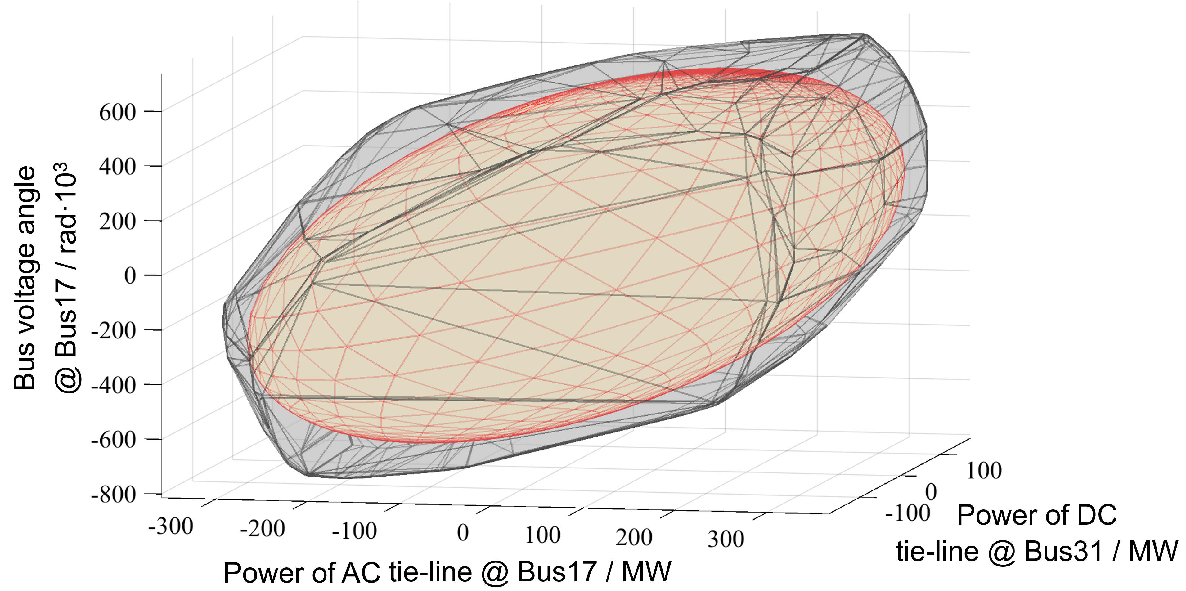
Figure 8: Coupling relationship among three boundary variables and inner-approximated flexibility region at time slice 12:00.

Taking the time slot at 12:00 as an example, the coupling relationship among the boundary variables, the power of the DC tie-line connected to Bus 31, the power of the AC tie-line connected to Bus 17, and the voltage angle of Bus 17, are shown in Fig. 8. The ellipsoid represents the inner-approximated flexibility region with an ellipsoidal shape template. The gray polytope represents the actual flexibility region obtained by searching for all extreme points. The practical RPG may have far more tie-lines, making it intractable to find all the extreme points of the actual flexibility region as in this case. Therefore, the ellipsoidal shape template is a convenient tool to self-adaptively inner-approximate the flexibility region with fewer parameters.

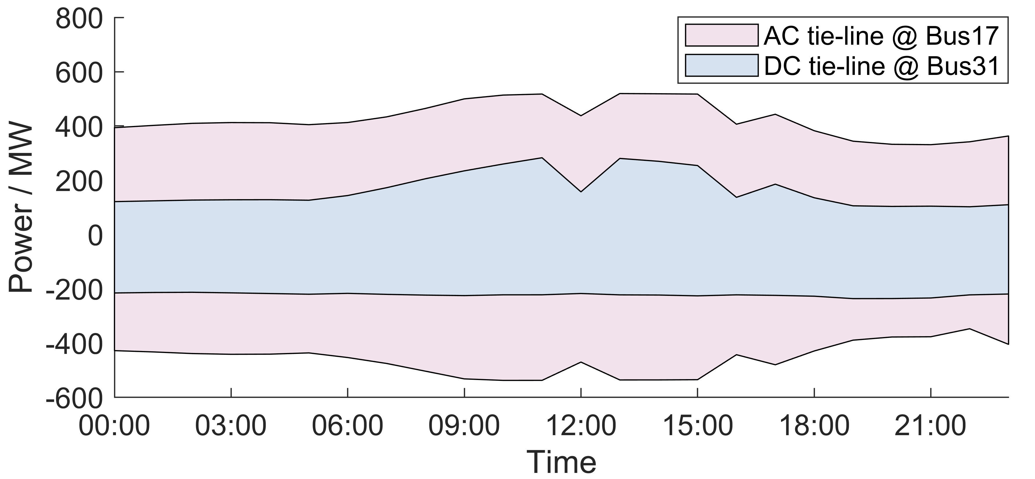
Figure 9: Power bounds of two tie-lines in IEEE 118 RPG.

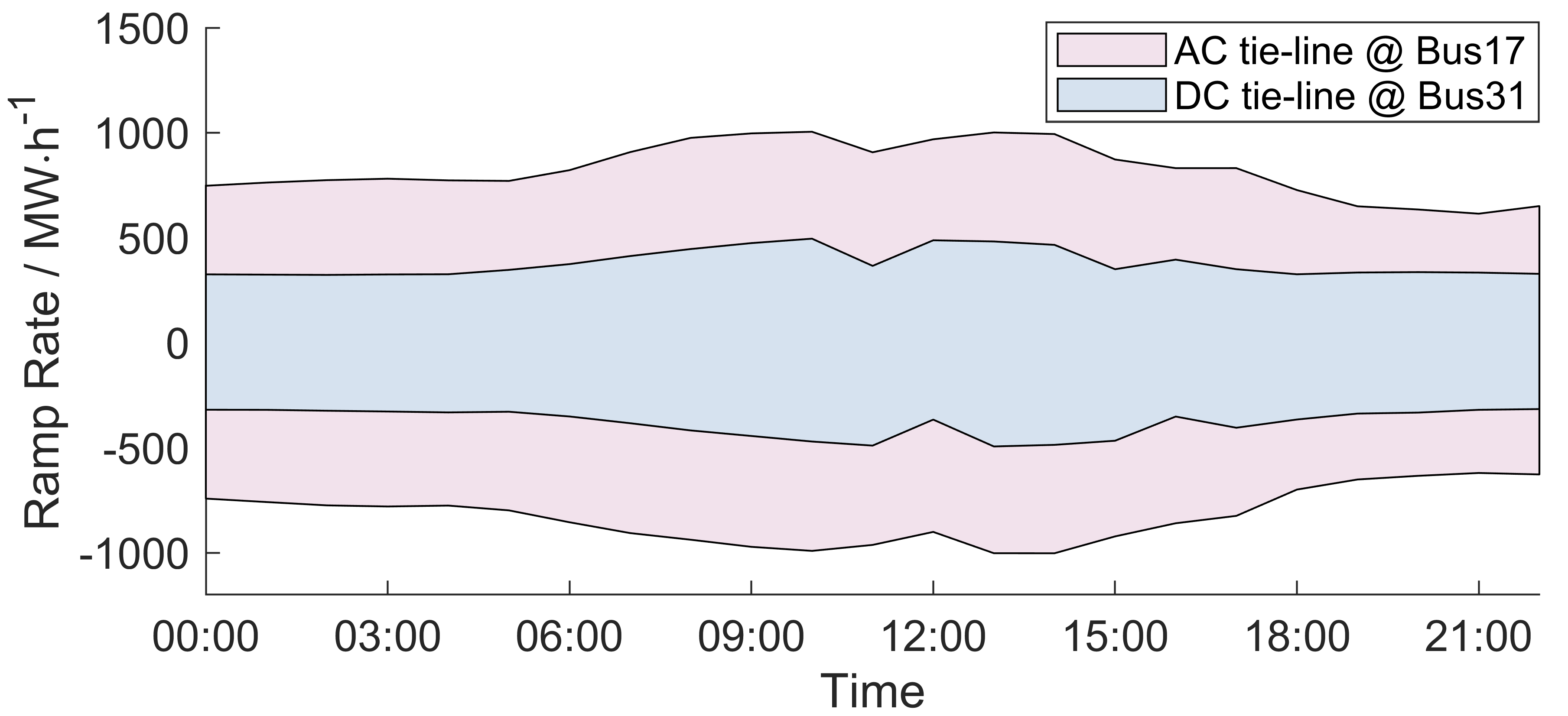
Figure 10: Ramp rate bounds of two tie-lines in IEEE 118 RPG.

In addition, the temporal coupling flexibility region across all time slots including the power and ramp rate bounds of these two tie-lines are shown in Fig. 9 and 10. The power and ramp rate limits can also be viewed as the parameters of the equivalent generators connected to these two tie-lines as illustrated in the physical counterpart in Fig. 7.

The aggregated cost function with the output power of two tie-lines as variables at 12:00 is shown in Fig. 11.

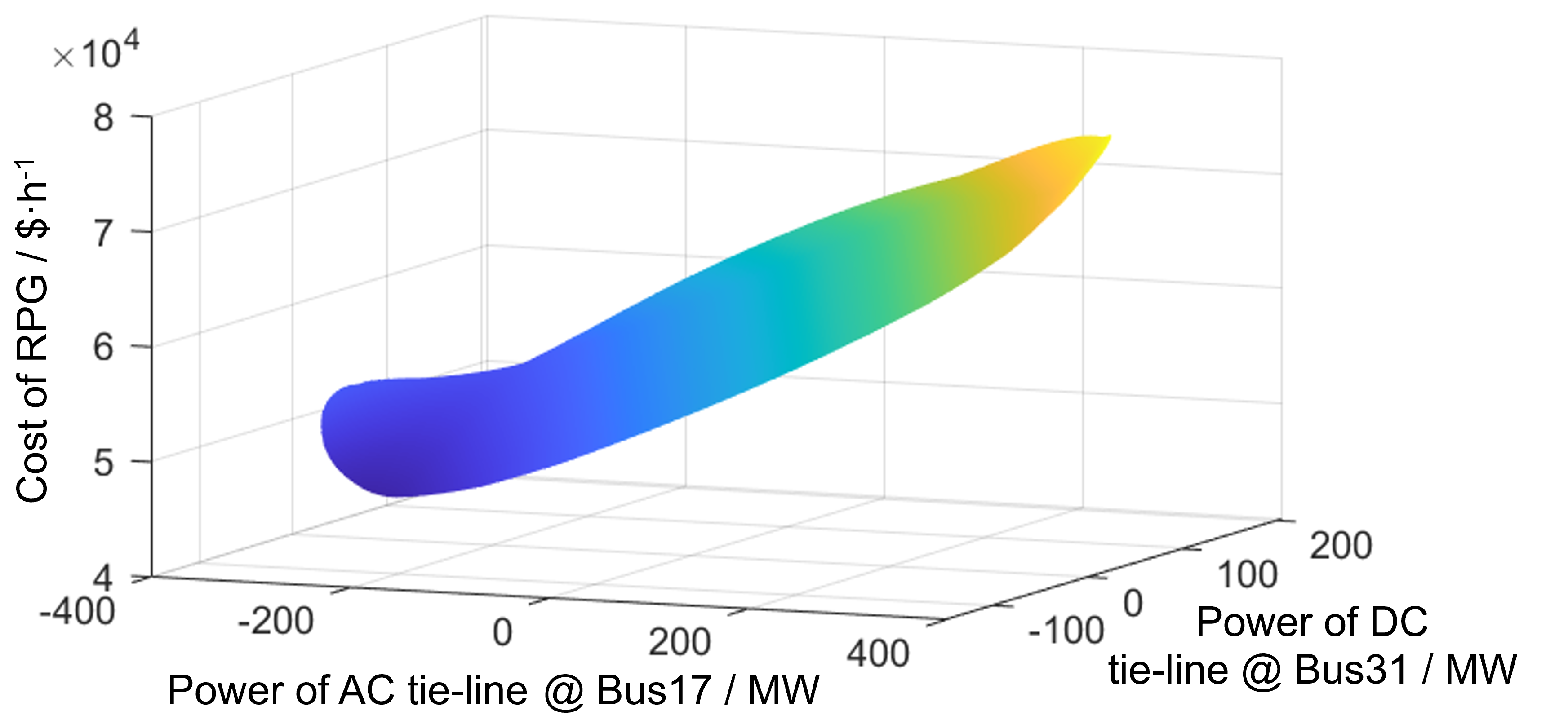
Figure 11: Aggregated cost function of IEEE 118 RPG.

VI-C Coordinated Dispatch Results of Five-Region European Power Grids

The five-region European power grid is shown in Fig. 12, with the detailed parameters listed in the supplemental file [26].

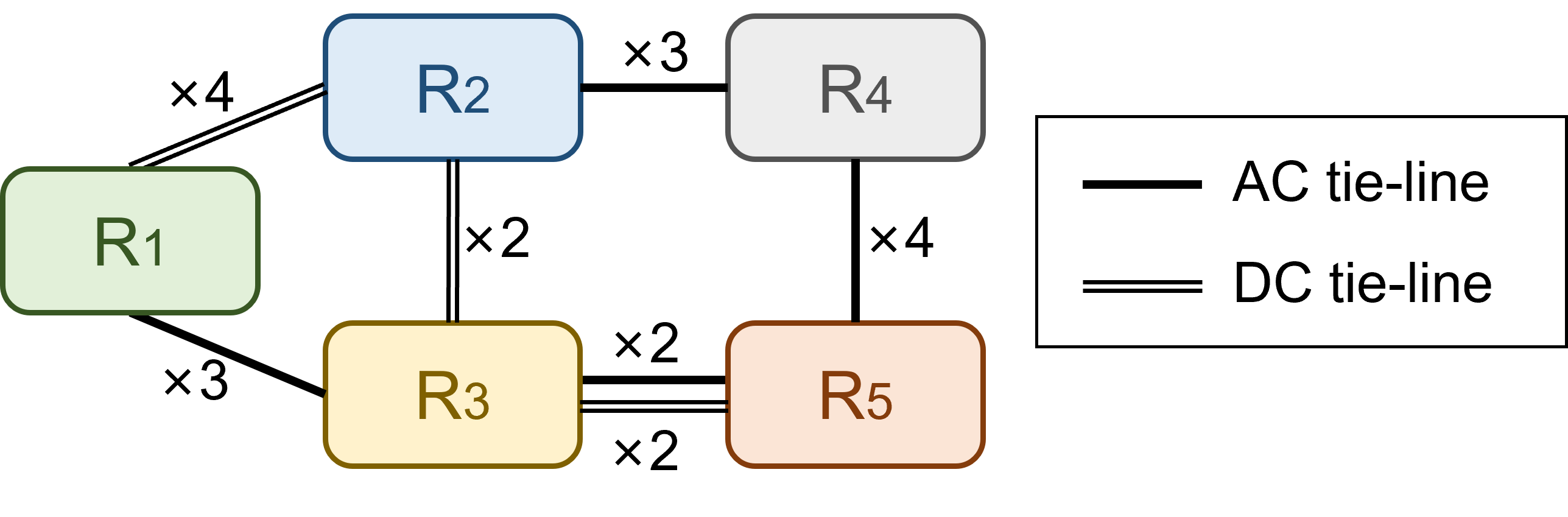
Figure 12: The five-region interconnected power grid.

The aggregated models of these five-region European RPGs can be calculated with the proposed method. Taking the RPG R1 as an example, the power and ramp rate bounds of its seven tie-lines are shown in Fig. 13.

Figure 13: Aggregation results of RPG R1: (a) Power bounds; (b) Ramp rate bounds.

Using the flexibility aggregation models of these five RPGs, the coordinated dispatch results for the interconnected power grid can be achieved in a non-iterative manner. Fig. 14 illustrates the power transmission between RPGs via tie-lines. The dotted lines represent the coordinated results obtained using the flexibility aggregation models in non-iterative method, while the solid lines depict the results from the distributed iterative dispatch.

Figure 14: Coordinated dispatch results of the five-region European power grid.

According to Fig. 14, errors are present when using the flexibility aggregation models in non-iterative method. The errors mainly come from two aspects: the inner approximation errors between the flexibility aggregation models and the actual flexibility region, and the mismatch between the fitted cost function and the actual cost function. Despite these inaccuracies, the flexibility aggregation model-based coordination results can provide a good initial value for further iterative method’s distributed coordination calculations. This accelerates the convergence of the distributed algorithm and helps mitigate the risk of divergence in the distributed coordinated scheduling process.

VI-D Comparison with Existing Aggregation Methods

In this section, the performance of the proposed method is compared with the existing methods, including vertex search [8], multi-parametric programming [11], Fourier-Motzkin elimination [6], cubic inner approximation [12] and temporal dimension decomposition [3]. The regional power grid R1 is used as the test case. The above methods are applied to calculate the flexibility aggregation results, respectively. Furthermore, to compare the performance of the aggregated flexibility region of the RPG, the scenario coverage rate metric is used. This metric is defined as the proportion of the 100,000 operational scenarios that meet all technical constraints and are covered by the aggregated flexibility region. It serves as an indicator of the similarity between the calculated flexibility region and the actual flexibility region.

Due to the high-dimensional nature of this aggregation problem, methods like vertex search, multi-parametric programming, and Fourier-Motzkin elimination suffer from the curse of dimensionality and are unable to complete the calculation within one hour. The comparison results of other methods are shown in TABLE I.

TABLE I: Comparison of the Flexibility Aggregation Results

Method	Computation time / s	Scenario coverage rate
Cubic inner approximation [12]	243	36.72%
Temporal dimension decomposition [3]	673	69.87%
Our method	617	85.49%

The cubic inner approximation method [12] provides much faster computation speed by using a simple cubic shape template to inner-approximate the real flexibility region. The temporal dimension decomposition method [3] and our proposed method, while slower, offer a more accurate representation of the aggregated flexibility region. In addition, compared to the time-dimension decomposition method, our proposed method in this paper achieves a more precise inner approximation of the flexibility region by incorporating the ramping characteristics of tie-lines.

VII Conclusion

This paper introduces a dimension-decomposition-based inner approximation method for flexibility aggregation of regional power grids with multiple AC and DC tie-lines. The aggregated model integrates the detail models of internal devices and operation constraints, facilitating optimal coordination across interconnected power grids in a non-iterative way.

To accelerate the calculation of aggregated model, enhance the coverage of the flexibility region, and derive physically meaningful flexibility aggregation results, this method incorporates three key strategies: (i) decomposing the high-dimensional flexibility aggregation region into subspaces based on the analysis of the coupling relationships among boundary variables; (ii) solving the projection problem within each subspace independently and in parallel; and (iii) employing appropriate shape templates to inner-approximate the flexibility regions.

Numerical tests demonstrate that this flexibility aggregation method is significantly less conservative than existing methods, while reliably ensuring the feasibility of the aggregated results in the dispatch process of each regional power grid.

References

- [1] H. Zhang, X. Hu, H. Cheng, S. Zhang, S. Hong, and Q. Gu, “Coordinated scheduling of generators and tie lines in multi-area power systems under wind energy uncertainty,” Energy, vol. 222, p. 119929, May 2021.
- [2] W. Lin, Z. Yang, J. Yu, K. Xie, X. Wang, and L. Wenyuan, “Tie-Line Security Region Considering Time Coupling,” IEEE Transactions on Power Systems, vol. 36, no. 2, pp. 1274–1284, Mar. 2021.
- [3] W. Lin, H. Jiang, H. Jian, J. Xue, J. Wu, C. Wang, and Z. Lin, “High-dimension tie-line security regions for renewable accommodations,” Energy, vol. 270, p. 126887, May 2023.
- [4] Z. Tan, Z. Yan, H. Zhong, and Q. Xia, “Non-Iterative Solution for Coordinated Optimal Dispatch via Equivalent Projection—Part II: Method and Applications,” IEEE Transactions on Power Systems, vol. 39, no. 1, pp. 899–908, Jan. 2024.
- [5] G. B. Dantzig, B. C. Eaves et al., “Fourier-Motzkin elimination and its dual,” J. Comb. Theory, Ser. A, vol. 14, no. 3, pp. 288–297, 1973.
- [6] A. A. Jahromi and F. Bouffard, “On the Loadability Sets of Power Systems—Part I: Characterization,” IEEE Transactions on Power Systems, vol. 32, no. 1, pp. 137–145, Jan. 2017.
- [7] W. Wei, F. Liu, and S. Mei, “Dispatchable Region of the Variable Wind Generation,” IEEE Transactions on Power Systems, vol. 30, no. 5, pp. 2755–2765, 2015.
- [8] Z. Tan, H. Zhong, J. Wang, Q. Xia, and C. Kang, “Enforcing Intra-Regional Constraints in Tie-Line Scheduling: A Projection-Based Framework,” IEEE Transactions on Power Systems, vol. 34, no. 6, pp. 4751–4761, Nov. 2019.
- [9] W. Lin, Z. Yang, J. Yu, G. Yang, and L. Wen, “Determination of Transfer Capacity Region of Tie Lines in Electricity Markets: Theory and Analysis,” Applied Energy, vol. 239, pp. 1441–1458, Apr. 2019.
- [10] W. Lin, Z. Yang, J. Yu, L. Jin, and W. Li, “Tie-Line Power Transmission Region in a Hybrid Grid: Fast Characterization and Expansion Strategy,” IEEE Transactions on Power Systems, vol. 35, no. 3, pp. 2222–2231, May 2020.
- [11] W. Dai, Z. Yang, J. Yu, K. Zhao, S. Wen, W. Lin, and W. Li, “Security region of renewable energy integration: Characterization and flexibility,” Energy, vol. 187, p. 115975, Nov. 2019.
- [12] X. Chen and N. Li, “Leveraging Two-Stage Adaptive Robust Optimization for Power Flexibility Aggregation,” IEEE Transactions on Smart Grid, vol. 12, no. 5, pp. 3954–3965, Sep. 2021.
- [13] B. Cui, A. Zamzam, and A. Bernstein, “Network-Cognizant Time-Coupled Aggregate Flexibility of Distribution Systems Under Uncertainties,” IEEE Control Systems Letters, vol. 5, no. 5, pp. 1723–1728, Nov. 2021.
- [14] H. Zhao, B. Wang, Z. Pan, H. Sun, Q. Guo, and Y. Xue, “Aggregating Additional Flexibility from Quick-Start Devices for Multi-Energy Virtual Power Plants,” IEEE Transactions on Sustainable Energy, vol. 12, no. 1, pp. 646–658, Jan. 2020.
- [15] S. Wang and W. Wu, “Aggregate Flexibility of Virtual Power Plants with Temporal Coupling Constraints,” IEEE Transactions on Smart Grid, vol. 12, no. 6, pp. 5043–5051, Nov. 2021.
- [16] Y. Wen, Z. Hu, S. You, and X. Duan, “Aggregate Feasible Region of DERs: Exact Formulation and Approximate Models,” IEEE Transactions on Smart Grid, vol. 13, no. 6, pp. 4405–4423, Nov. 2022.
- [17] E. Dall’Anese, P. Mancarella, and A. Monti, “Unlocking Flexibility: Integrated Optimization and Control of Multienergy Systems,” IEEE Power and Energy Magazine, vol. 15, no. 1, pp. 43–52, Jan. 2017.
- [18] G. Chicco, S. Riaz, A. Mazza, and P. Mancarella, “Flexibility From Distributed Multienergy Systems,” Proceedings of the IEEE, vol. 108, no. 9, pp. 1496–1517, Sep. 2020.
- [19] S. Wang, “Flexibility Aggregation and Coordination of Diverse Energy Resources,” Ph.D. dissertation, Tsinghua University, Tsinghua University, May 2024.
- [20] J. Zhen, “Computing the Maximum Volume Inscribed Ellipsoid of a Polytopic Projection,” INFORMS Journal on Computing, vol. 30, no. 1, pp. 31–42, 2018.
- [21] Y. Wen, Z. Hu, J. He, and Y. Guo, “Improved Inner Approximation for Aggregating Power Flexibility in Active Distribution Networks and Its Applications,” IEEE Transactions on Smart Grid, vol. 15, no. 4, pp. 3653–3665, Jul. 2024.
- [22] X. Chen, E. Dall’Anese, C. Zhao, and N. Li, “Aggregate Power Flexibility in Unbalanced Distribution Systems,” IEEE Transactions on Smart Grid, vol. 11, no. 1, pp. 258–269, Jan. 2020.
- [23] S. Wang, W. Wu, Q. Chen, J. Yu, and P. Wang, “Stochastic Flexibility Evaluation for Virtual Power Plants by Aggregating Distributed Energy Resources,” CSEE Journal of Power and Energy Systems, vol. 10, no. 3, pp. 988–999, May 2024.
- [24] Y. Yang, W. Wu, B. Wang, and M. Li, “Analytical Reformulation for Stochastic Unit Commitment Considering Wind Power Uncertainty With Gaussian Mixture Model,” IEEE Transactions on Power Systems, vol. 35, no. 4, pp. 2769–2782, Jul. 2020.
- [25] C. Ordoudis, V. A. Nguyen, D. Kuhn, and P. Pinson, “Energy and reserve dispatch with distributionally robust joint chance constraints,” Operations Research Letters, vol. 49, no. 3, pp. 291–299, May 2021.
- [26] S. Wang, “Supplemental File for Non-Iterative Coordination of Interconnected Power Grids via Dimension Decomposition-Based Flexibility Aggregation,” https://github.com/wangsyTHU/SupplementaryFiles/tree/master/RPGAgg, Nov. 2024.
- [27] F. Capitanescu, “Computing Cost Curves of Active Distribution Grids Aggregated Flexibility for TSO-DSO Coordination,” IEEE Transactions on Power Systems, vol. 39, no. 1, pp. 2381–2384, Jan. 2024.
- [28] A. Magnani and S. P. Boyd, “Convex piecewise-linear fitting,” Optimization and Engineering, vol. 10, no. 1, pp. 1–17, Mar. 2009.
- [29] R. D. Zimmerman, C. E. Murillo-Sánchez, and R. J. Thomas, “MATPOWER: Steady-State Operations, Planning, and Analysis Tools for Power Systems Research and Education,” IEEE Transactions on Power Systems, vol. 26, no. 1, pp. 12–19, Feb. 2011.
- [30] “California ISO - Historical EMS Hourly Load,” https://www.caiso.com/Documents.
- [31] D. Jager and A. Andreas, “NREL National Wind Technology Center (NWTC): M2 Tower; Boulder, Colorado (Data),” 1996.
- [32] J. Lofberg, “YALMIP : A toolbox for modeling and optimization in MATLAB,” in 2004 IEEE International Conference on Robotics and Automation (IEEE Cat. No.04CH37508). Taipei, Taiwan: IEEE, 2004, pp. 284–289.
- [33] M. Herceg, M. Kvasnica, C. N. Jones, and M. Morari, “Multi-Parametric Toolbox 3.0,” in Proc. of the European Control Conference, Zürich, Switzerland, Jul. 2013, pp. 502–510.
- [34] D. Ge, Q. Huangfu, Z. Wang, J. Wu, and Y. Ye, “Cardinal Optimizer (COPT) user guide,” 2022.
- [35] Gurobi Optimization, LLC, “Gurobi Optimizer Reference Manual,” 2024.