Enhancing Physics-Informed Neural Networks Through Feature Engineering

Abstract

Physics-Informed Neural Networks (PINNs) seek to solve partial differential equations (PDEs) with deep learning. Mainstream approaches that deploy fully-connected multi-layer deep learning architectures require prolonged training to achieve even moderate accuracy, while recent work on feature engineering allows higher accuracy and faster convergence. This paper introduces SAFE-NET, a Single-layered Adaptive Feature Engineering NETwork that achieves orders-of-magnitude lower errors with far fewer parameters than baseline feature engineering methods. SAFE-NET returns to basic ideas in machine learning, using Fourier features, a simplified single hidden layer network architecture, and an effective optimizer that improves the conditioning of the PINN optimization problem. Numerical results show that SAFE-NET converges faster and typically outperforms deeper networks and more complex architectures. It consistently uses fewer parameters—on average, 65% fewer than the competing feature engineering methods—while achieving comparable accuracy in less than 30% of the training epochs. Moreover, each SAFE-NET epoch is 95% faster than those of competing feature engineering approaches. These findings challenge the prevailing belief that modern PINNs effectively learn features in these scientific applications and highlight the efficiency gains possible through feature engineering.

1 Introduction

Partial Differential Equations (PDEs) underpin scientific modeling but remain notoriously challenging to solve. Classical numerical methods struggle with high dimensionality and nonlinearity, while analytical solutions are rare. Physics-Informed Neural Networks (PINNs) (Raissi et al., 2019; Karniadakis et al., 2021) have emerged as a promising alternative, leveraging neural networks to approximate PDE solutions through residual minimization. By avoiding mesh generation, PINNs offer flexibility for forward/inverse problems and high-dimensional settings.

Despite their potential, PINNs face a fundamental challenge—they are difficult to train (Krishnapriyan et al., 2021; Rathore et al., 2024). The differential operator in the residual loss induces ill-conditioning (De Ryck et al., 2023; Rathore et al., 2024), leading to a poor optimization landscape and slow convergence for popular first-order optimizers such as Adam (Kingma & Ba, 2014). Thus, successful PINN training can be time-consuming and fiddly, limiting the use of PINNs.

Recent work has developed several strategies to improve PINN training, including feature engineering. Feature engineering endows the network with additional features that better capture the inductive bias of the learning task. A range of feature engineering approaches, from Fourier features (RFF-PINNs) (Wang et al., 2020) to radial basis function features (RBF-PINN) (Zeng et al., 2024a), have been proposed.

However, prior work on feature engineering generally suffers from one or more of the following four limitations: 1) they impose rigid priors (e.g. the features are fixed or random functions), 2) they require hyperparameter tuning (e.g. determining kernel hyperparameters in RBF-PINNs), 3) they are often computationally expensive, and 4) they fail to integrate domain knowledge such as boundary or initial conditions. Thus, while existing feature engineering techniques can improve performance under certain conditions, they can be PDE-specific, expensive, and sensitive to hyperparameters.

Figure 1: L2RE for the Heat PDE with SAFE-NET and baselines.

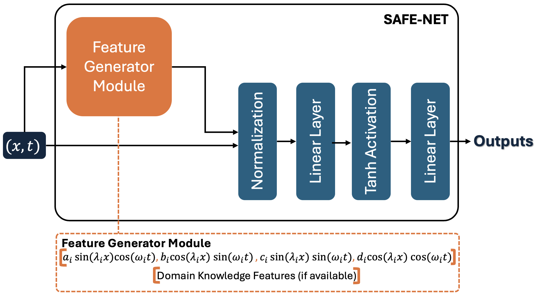
To address these shortcomings we introduce SAFE-NET, a feature engineering framework for PINNs that combines:

• Well-conditioned adaptive Fourier basis terms as features with trainable frequencies $\omega_{x}$, $\lambda_{t}$ and amplitudes adapt to PDE-specific dominant frequencies while mitigating spectral bias.

• Domain knowledge features encode physical priors, derived from boundary conditions or initial conditions.

• Normalization of features prior to network input stabilizes quasi-Newton optimizers (e.g., L-BFGS) and other advanced optimizers and prevents divergence. Many other methods introduce sensitive architectural or problem-related hyperparameters or features, causing instability across some of our tested PDEs. In other words, SAFE-NET can safely be optimized by high-performance optimizers.

SAFE-NET does not directly target the optimization landscape like prior feature engineering approaches such as RFF-PINNs or RBF-PINNs. Instead, it seeks to improve the inductive bias of the PINN by augmenting the initial data representation with well-conditioned Fourier features and domain knowledge. These design choices makes SAFE-NET particularly effective for PDEs without shocks or discontinuities, where Fourier bases work best. Interestingly, this inductive bias also provides an implicit preconditioning effect that leads to a better-conditioned optimization problem and facilitates training.

Contributions. We highlight the contributions of this paper:

• Our new computationally-efficient feature engineering method, SAFE-NET, offers better inductive bias than existing feature engineering methods.

• We demonstrate empirically and theoretically that SAFE-NET implicitly preconditions the loss landscape, leading to faster, more stable convergence.

• SAFE-NET achieves runtime performance comparable to non-feature engineering methods, while other feature engineering approaches are slower (Table 1 and Figure 4).

• Experiments across a wide variety of PDEs and baseline methods (Table 2) show that SAFE-NET yields the best or comparable performance.

Deep learning has been seen as a promising tool for solving PDEs. However, our work with SAFE-NET shows that traditional techniques like feature engineering can achieve lower error rates and faster training times than conventional multi-layer networks. This achievement suggests that for PDE tasks, feature engineering can be more effective than adding complexity to the network, challenging the common belief that deeper networks effectively learn important problem features.

2 Insights into Feature Engineering in PINNs

This section explores the two primary approaches to feature engineering, Fourier-based and non-Fourier feature mappings. To better understand the advantages SAFE-NET offers, we highlight the strengths, limitations, and applicability of these approaches to different PDE classes.

2.1 Fourier-Based Feature Engineering

Fourier feature mappings leverage the spectral properties of PDE solutions to enhance high-frequency learning. They aim to address spectral bias — the tendency of neural networks to favor low-frequency functions — by transforming input coordinates into a more expressive representation. The most prominent approach, RFF-PINN (Wang et al., 2021b), uses the feature mapping

$$\gamma(v)=\big{[}\cos(Bv),\sin(Bv)\big{]},$$ (1)

with fixed Gaussian weights $B\in\mathbb{R}^{m\times d}$ drawn from $\mathcal{N}(0,\sigma^{2})$. With both cosine and sine terms, this mapping projects inputs into a high-dimensional space where periodic and high-frequency patterns are more easily captured. Theoretical insights from (Tancik et al., 2020) show that Fourier features help neural networks learn high-frequency functions in low-dimensional domains, which are typical in PDE applications. However, RFF-PINN’s reliance on fixed, random frequencies limits its adaptation to PDE-specific spectral properties. Moreover, the Gaussian initialization of $B$ may not align with the dominant frequencies of the solution, leading to reduced performance.

2.2 Non-Fourier Approaches

For PDEs with sharp gradients or discontinuities, Fourier features may struggle due to the Gibbs phenomenon; see (Zeng et al., 2024b). The Burgers PDE, with its sharp discontinuity at $x=0$, is well-suited to observe this behavior. Comparing numerical results for the Burgers PDE across methods in Table 3 show that RFF-PINN performs comparably to methods without feature engineering but underperforms RBF-PINN by over an order of magnitude.

(Zeng et al., 2024a) addresses the Gibbs phenomenon by using Radial Basis Functions (RBFs) as

$$\phi_{\text{RBF}}(x)=\exp\!\Bigl{(}-\tfrac{\lvert x-c\rvert^{2}}{2\sigma^{2}}\Bigr{)},$$ (2)

where $c$ denotes the center and $\sigma$ controls the kernel width. RBF expansions can better approximate local, abrupt changes but are computationally intensive due to kernel regression requirements and less suited for periodic or high-frequency PDE solutions (Tancik et al., 2020).

2.3 Comparisons and Practical Considerations

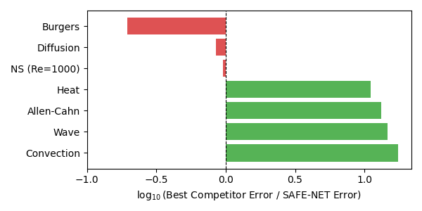
The choice between Fourier and non-Fourier features depends on PDE characteristics. Fourier features are ideal for smooth, periodic solutions but struggle with discontinuities. RBFs handle sharp discontinuities better but are computationally costly. SAFE-NET offers a sensible compromise, allowing trainable frequency parameters and domain-inspired features to improve inductive bias with a unified computationally-efficient design. Even for the Burgers equation, SAFE-NET significantly outperforms both non-feature-engineered and Fourier feature-based methods, maintaining a less-than-an-order-of-magnitude performance gap with RBF-PINN, as shown in Figure 3.

3 Methodology

We introduce SAFE-NET in this section. We begin with some motivation from Fourier analysis.

3.1 Theoretical Background

Let $f(\mathbf{x}):\mathbb{R}^{d}\to\mathbb{R}$ be a function defined on a $d$-dimensional domain. Under mild regularity conditions, $f(\mathbf{x})$ can be reconstructed from its Fourier transform using the inverse Fourier transform $f(\mathbf{x})=\int_{-\infty}^{\infty}\hat{f}(\mathbf{\kappa})e^{2\pi i\mathbf{\kappa}\cdot\mathbf{x}}\,d\mathbf{\kappa},$ where $\hat{f}(\mathbf{\kappa})$ is the Fourier transform of $f$ at frequency $\kappa$. To approximate $f$, we can focus on the dominant frequencies with large $|\hat{f}(\mathbf{\kappa})|$. Summing over these dominant frequencies, we obtain $f(\mathbf{x})\approx\sum_{\mathbf{\kappa}\text{ dominant}}\hat{f}(\mathbf{\kappa})e^{2\pi i\mathbf{\kappa}\cdot\mathbf{x}}.$ We can express the Fourier transform $\hat{f}(\mathbf{\kappa})$ through its real and imaginary components to rewrite the approximation as

$$f(\mathbf{x})\approx\sum_{\mathbf{\kappa}\text{ dominant}}\left(A_{\mathbf{\kappa}}\cos(2\pi\mathbf{\kappa}\cdot\mathbf{x})+B_{\mathbf{\kappa}}\sin(2\pi\mathbf{\kappa}\cdot\mathbf{x})\right),$$

where $A_{\mathbf{\kappa}}$ and $B_{\mathbf{\kappa}}$ are real-valued coefficients derived from $\hat{f}(\mathbf{\kappa})$. Fourier basis elements are effective as features when they include the dominant frequencies $\kappa$ of $f(\mathbf{x})$.

Figure 2: Diagram showing how SAFE-NET works for a 1D time-dependent PDE as an example. The Feature Generator Module has trainable frequencies and coefficient for more effective feature selection.

For a PDE solution $u(x,t):\mathbb{R}^{2}\to\mathbb{R}$, the 2D Fourier transform and its inverse are given by

$$\hat{u}(\omega_{x},\lambda_{t}) =\iint_{\mathbb{R}^{2}}u(x,t)e^{-2\pi i(\omega_{x}x+\lambda_{t}t)}dxdt,$$

$$u(x,t) =\iint_{\mathbb{R}^{2}}\hat{u}(\omega_{x},\lambda_{t})e^{2\pi i(\omega_{x}x+\lambda_{t}t)}d\omega_{x}d\lambda_{t},$$

where $(\omega_{x},\lambda_{t})$ are spatial and temporal frequencies. Expanding the complex exponential yields the tensor product basis

$$e^{2\pi i(\omega_{x}x+\lambda_{t}t)} =e^{2\pi i\omega_{x}x}\otimes e^{2\pi i\lambda_{t}t}$$

$$=\begin{aligned} \big{[}\cos(2\pi\omega_{x}x)+i\sin(2\pi\omega_{x}x)\big{]}\\ \otimes\big{[}\cos(2\pi\lambda_{t}t)+i\sin(2\pi\lambda_{t}t)\big{]}.\end{aligned}$$

This expansion produces four real-valued basis functions per frequency pair $(\omega_{x},\lambda_{t})$ as

$$\phi_{1}^{\omega_{x},\lambda_{t}}(x,t) =\cos(\omega_{x}x)\cos(\lambda_{t}t)$$ (3)

$$\phi_{2}^{\omega_{x},\lambda_{t}}(x,t) =\sin(\omega_{x}x)\cos(\lambda_{t}t)$$ (4)

$$\phi_{3}^{\omega_{x},\lambda_{t}}(x,t) =\cos(\omega_{x}x)\sin(\lambda_{t}t)$$ (5)

$$\phi_{4}^{\omega_{x},\lambda_{t}}(x,t) =\sin(\omega_{x}x)\sin(\lambda_{t}t).$$ (6)

3.2 SAFE-NET

Motivated by the considerations of Section 3.1, SAFE-NET implements the parametric basis in equations (3)-(6) through learnable frequencies $\{\omega_{x}^{(i)},\lambda_{t}^{(i)}\}_{i=1}^{N}$ and amplitudes $\{a^{(i)},b^{(i)},c^{(i)},d^{(i)}\}_{i=1}^{N}$ to estimate

$$u_{\theta}(x,t) =\sum_{i=1}^{N}\big{[}a^{(i)}\phi_{1}^{\omega_{x},\lambda_{t}}(x,t)+b^{(i)}\phi_{2}^{\omega_{x},\lambda_{t}}(x,t)$$

$$\quad+c^{(i)}\phi_{3}^{\omega_{x},\lambda_{t}}(x,t)+d^{(i)}\phi_{4}^{\omega_{x},\lambda_{t}}(x,t)\big{]}$$ (7)

where $\theta=\{\omega_{x}^{(i)},\lambda_{t}^{(i)},a^{(i)},b^{(i)},c^{(i)},d^{(i)}\}$ are trainable parameters. The explicit cross-frequency terms in equation (7) capture the tensor product structure of the 2D Fourier basis.

Domain Knowledge Features. The solution $u(x,t)$ to a PDE often inherits structure from the domain geometry, boundary conditions, and physical invariants. SAFE-NET can explicitly encode this domain knowledge through features $\psi(x,t)$ automatically derived from boundary conditions, initial conditions, and known solution patterns for each PDEs in the feature generator module. For example, $\psi_{\text{wave}}=\{\sin(\pi x),\sin(5\pi x)\}$ and $\psi_{\text{heat}}=\{2-x,x^{2},x^{2}(2-x)\}$ are automatically included in SAFE-NET’s feature generator module, which come from the initial and boundary information. Features for the PDEs considered in this paper appear in Appendix B.

As shown in Figure 2, depending on the availability of domain information, these features are concatenated with the Fourier basis terms before normalization and linear projection. SAFE-NET uses only one hidden layer: given an input $(\bm{x},t)\in\Omega\times\mathbb{R}$, the SAFE-NET network computes

$$f_{\theta}(\bm{x},t)=w_{2}^{T}\sigma(W_{1}\phi(w_{\textup{SF-NET}},(\bm{x},t))+b_{1})+b_{2},$$ (8)

with parameters $\theta=(w_{\textup{SF-NET}},W_{1},b_{1},w_{2},b_{2})$, nonlinearity $\sigma=\tanh(\cdot),$ and learnable feature mapping $\phi(w_{\textup{SF-NET}},(\bm{x},t))$; see Appendix A.2 for details.

By combining the generality of Fourier features with known solution characteristics, SAFE-NET accelerates convergence. Figure 3 compares SAFE-NET with the best competing PINN architecture for each PDE in Table 2. SAFE-NET either yields the best performance or is comparable to the method that gives the best performance, highlighting SAFE-NET’s effectiveness.

Figure 3: Performance comparison of SAFE-NET against the best competitor method across various PDEs. SAFE-NET consistently ranks first or second, with larger order-of-magnitude improvements when leading (green bars) and smaller gaps otherwise (red bars).

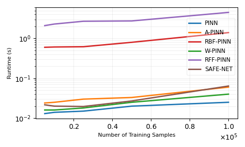
Cost. Table 1 and Figure 4 illustrate the parameter count and runtime (per epoch) for different baseline methods. The setups used for each method in our experiments appear in Appendix C. One hidden layer suffices for SAFE-NET, reducing its parameter count and improving speed.

Table 1: Parameter count comparison between baseline methods and SAFE-NET. Using the same number of features (128), SAFE-NET achieves a significantly lower parameter count than competing feature engineering methods while remaining comparable to non-feature engineering approaches.

PINN	A-PINN	W-PINN
$5.3$k	$5.3$k	$5.3$k
RBF-PINN	RFF-PINN	SAFE-NET
$14.2$k	$14.5$k	$5.8$k

Figure 4: Average runtime comparison across varying numbers of training samples for baseline methods and SAFE-NET using identical computational resources and no concurrent processes. SAFE-NET demonstrates superior efficiency over competing feature engineering methods, maintaining runtime close to the less computationally expensive non-feature engineering approaches

Scalability. The number of additional features in SAFE-NET increases exponentially with the spatial dimension of the PDE. Hence SAFE-NET offers improves accuracy and computational advantages for lower-dimensional problems, where better coverage of frequency space improves approximation quality, but is not suited to problems with high dimensions. Developing effective feature engineering methods for higher dimensional PINNS is an important challenge for future work.

4 Related work

Much work has been done to improve the training of PINNs that take different approaches from feature engineering. Broadly, these approaches can be divided into three categories: architectural modifications, loss-reweighting, and optimizer design. Recent efforts to improve PINN accuracy and speed include:

Architectural Modifications. One way to improve the training procedure for PINNs is to modify the network architecture, improving the optimization landscape relative to the basic PINN, making training easier. Examples of this approach include the adapative activation functions of (Jagtap et al., 2020) (A-PINNs), and specialized architectures designed to mitigate spectral bias (Li et al., 2020a).

Loss Re-weighting. Another popular technique is loss reweighting. For certain PDEs, the residual loss tends to dominate the boundary loss in that the optimizer focuses too much on minimizing the residual loss, leading to a solution that fails to satisfy the boundary conditions. To address this, techniques like W-PINNs (Wang et al., 2021a) balance loss components through heuristic or learned weights to down-weight the residual loss and better fit the boundary loss.

Optimizer Design. Another popular approach to PINN training is to develop more sophisticated optimizers that are more robust to ill-conditioning. Several notable proposals in this area are the natural gradients method of (Müller & Zeinhofer, 2023), MultiAdam (Yao et al., 2023), and NysNewton-CG (Rathore et al., 2024). These methods target ill-conditioning directly and use curvature information from the loss or the model to precondition the gradient. This leads to an improved optimization landscape locally, enabling the optimizer to take better steps and progress faster. In contrast, SAFE-NET enjoys an implicit preconditioning effect that is global—by incorporating a trainable feature layer, SAFE-NET changes the PINN objective, globally changing the optimization landscape. The results in Section 5.3 show SAFE-NET enjoys a significantly better-conditioned optimization landscape. Thus, SAFE-NET can be further combined with more sophisticated optimization schemes to obtain further improvements.

5 Results

We provide an overview of the experimental setup and present results across multiple benchmarks. More details on setups for each method appear in Appendix A.

5.1 Baselines

We test against PINN models with feature engineering (RBF-PINN, RFF-PINN) and without (PINN, W-PINN, A-PINN).

We do not test against operator learning methods such as Fourier Neural Operators (FNOs) (Li et al., 2020b) as they solve the inverse problem and require additional data while SAFE-NET and the baseline methods solve the forward problem. We experiment on the PDEs in Table 2.

Table 2: Overview of the tested PDEs.

PDE	Dimensions	Type	State
Wave	1D	Linear	Time-dependent
Heat	1D	Linear	Time-dependent
Convection	1D	Linear	Time-dependent
Diffusion	1D	Linear	Time-dependent
Burgers	1D	Nonlinear	Time-dependent
Allen-Cahn	2D	Nonlinear	Steady-state
Navier-Stokes	2D	Nonlinear	Steady-state

Throughout this text, we refer to the Steady state Navier-Stokes as NS (Re=1000) for short. Additional details on these PDEs are provided in Appendix B.

5.2 Experiments

Following prior work (e.g., (Wang et al., 2021b)), we use the Adam optimizer with a learning rate of 0.001 and an exponential decay rate of 0.9 every 2000 steps. Iteration counts typically range from 50,000 to 150,000, depending on problem complexity. For fairness, we train all methods, including SAFE-NET, for 150,000 epochs per problem, ensuring a generous comparison. Notably, while we maintain the same epoch count across all methods, SAFE-NET achieves faster per-epoch computation times compared to competing approaches, making its total training time more efficient in practice.

Table 3: PDE benchmark results comparing several PINN architectures in relative $L^{2}$ error. The best results are shown in bold.

PDE	PINN	A-PINN	W-PINN
Wave	$2.27\text{e}{-1}$	$7.23\text{e}{-2}$	$8.35\text{e}{-3}$
Diffusion	$1.43\text{e}{-3}$	$9.78\text{e}{-4}$	$8.65\text{e}{-4}$
Heat	$5.23\text{e}{-4}$	$1.12\text{e}{-4}$	$9.78\text{e}{-5}$
Convection	$2.78\text{e}{-3}$	$1.18\text{e}{-3}$	$8.67\text{e}{-4}$
Allen-Cahn	$1.12\text{e}{0}$	$8.66\text{e}{-1}$	$7.32\text{e}{-1}$
Burgers	$1.01\text{e}{-2}$	$3.34\text{e}{-3}$	$2.23\text{e}{-3}$
NS (Re=1000)	$4.49\text{e}{-1}$	$3.45\text{e}{-1}$	$4.99\text{e}{-1}$
PDE	RBF-PINN	RFF-PINN	SAFE-NET
Wave	$1.68\text{e}{-3}$	$6.61\text{e}{-3}$	$\boldsymbol{2.15\text{e}{-4}}$
Diffusion	$\boldsymbol{6.21\text{e}{-4}}$	$5.56\text{e}{-3}$	$7.32\text{e}{-4}$
Heat	$8.33\text{e}{-5}$	$3.56\text{e}{-4}$	$\boldsymbol{7.52\text{e}{-6}}$
Convection	$7.72\text{e}{-4}$	$1.02\text{e}{-3}$	$\boldsymbol{4.43\text{e}{-5}}$
Allen-Cahn	$9.37\text{e}{-2}$	$8.76\text{e}{-2}$	$\boldsymbol{6.65\text{e}{-3}}$
Burgers	$\boldsymbol{1.11\text{e}{-4}}$	${2.18\text{e}{-3}}$	$5.71\text{e}{-4}$
NS (Re=1000)	$\boldsymbol{1.98\text{e}{-1}}$	$5.76\text{e}{-1}$	$2.07\text{e}{-1}$

Table 3 demonstrates that for shock-free PDEs (i.e., not Burgers or NS), SAFE-NET outperforms competing methods in L2RE by an order of magnitude (Figure 3). For NS, SAFE-NET achieves error magnitudes matching the top baselines. For Burgers, SAFE-NET ranks second to RBF-PINN, surpassing all other baseline methods. This outcome is not surprising as SAFE-NET is not designed for PDEs with shocks. (Zeng et al., 2024b) suggests that the RBF kernel handles the discontinuity at $x=0$ in the Burgers equation more effectively. Figure 1 illustrates the performance of each method on the heat PDE as an example. Similar plots for other PDEs appear in Appendix C.

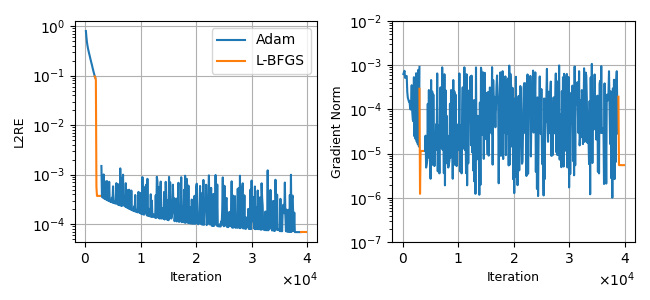
SAFE-NET is compatible with higher-accuracy optimizers: it can safely be optimized by quasi-Newton methods such as L-BFGS, which cause divergence or instability in other PINN variants for some PDEs. To demonstrate this claim, we evaluate SAFE-NET on the same PDEs using a combination of Adam and L-BFGS optimization strategy, $(\text{Adam}+\text{L-BFGS})^{2}$. This approach runs 3000 Adam iterations, switches to L-BFGS until convergence stalls, reverts to Adam and continues, and finally switches back to L-BFGS for the last 3000 epochs. Training is limited to 40,000 epochs — less than a third of previous experiments. The combination SAFE-NET + $(\text{Adam}+\text{L-BFGS})^{2}$ consistently matches or outperforms results in Table 1. Hyperparameter analysis in Appendix A.4 validates our optimizer choice. Notably, $(\text{Adam}+\text{L-BFGS})^{2}$ fails to improve ( and often degrades ) performance for the majority of the baseline methods across different PDEs, making it unsuitable to compare PINN architectures. See Appendix A.4 for details on how $(\text{Adam}+\text{L-BFGS})^{2}$ asffects the baseline methods.

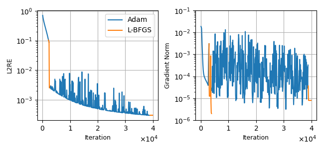
Figure 5 demonstrates the performance of SAFE-NET + $(\text{Adam}+\text{L-BFGS})^{2}$ on the wave and Allen-Cahn PDEs, presenting the gradient norm plots as well. Table 4 summarizes these numerical results, which shows an order of magnitude improvement for the wave, Allen-Cahn, Burgers, and NS PDEs; the others match the top results of Table 3.

(a)

(b)

Figure 5: L2RE and gradient norm for the wave and Allen-Cahn PDEs using SAFE-NET with (Adam + L-BFGS)².

Table 4: L2RE with SAFE-NET and different optimizers with equal average time budget (840 s)

PDE	Adam	(Adam + L-BFGS)²
Wave	$7.79\text{e}{-2}$	$7.05\text{e}{-5}$
Diffusion	$8.67\text{e}{-2}$	$6.13\text{e}{-4}$
Heat	$1.35\text{e}{-4}$	$4.93\text{e}{-6}$
Convection	$3.71\text{e}{-2}$	$6.26\text{e}{-5}$
Allen-Cahn	$1.46\text{e}{-1}$	$3.61\text{e}{-4}$
Burgers	$2.19\text{e}{-2}$	$6.97\text{e}{-5}$
NS	$8.69\text{e}{-1}$	$8.73\text{e}{-2}$

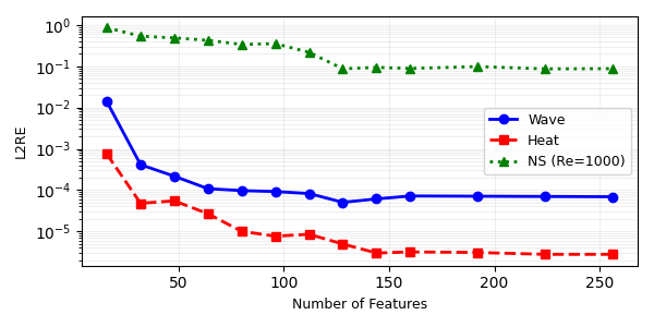
Figure 6 shows that on the wave, heat, and NS PDEs, the error gradually decreases as the number of SAFE-NET features increases until it reaches a saturation point (at around 120–140 features for these problems). This observation suggests that there is no advantage to adding additional features after a certain complexity is reached: they do not improve performance, but only increase the number of trainable parameters and computational cost. Detailed numerical results for other PDEs are provided in Table 6 in Appendix C.

Figure 6: L2RE decreases as number of features increases.

5.3 Feature Engineering and Spectral Density Analysis

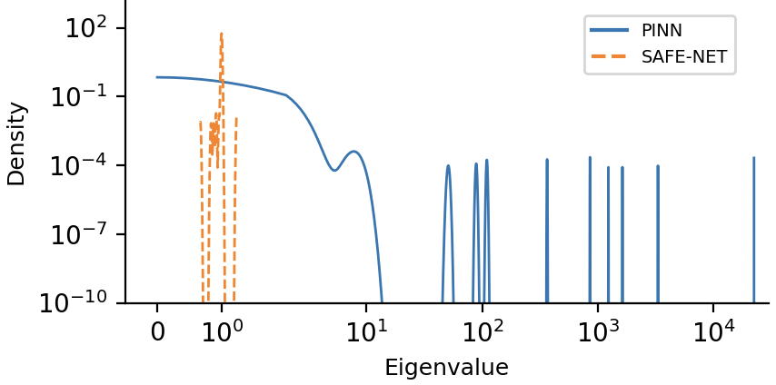
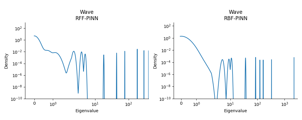
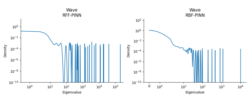
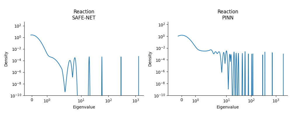
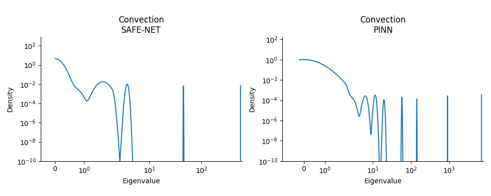
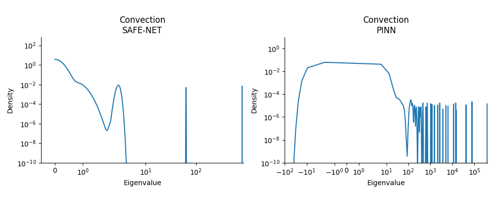
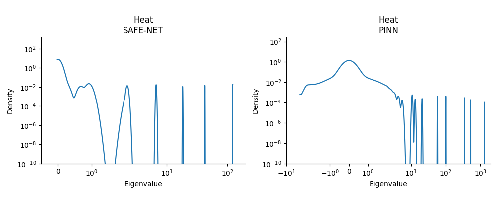
SAFE-NET significantly improves the conditioning of all tested PDEs. We analyze conditioning both at initialization (after 3000 Adam epochs) and post-training using SAFE-NET and PINN with (Adam+L-BFGS)² for 40,000 iterations, using the optimizer settings of the previous experiment. Figure 7 illustrates this for the wave PDE as an example; analogous plots for other PDEs are provided in Appendix C, alongside spectral density calculation details.

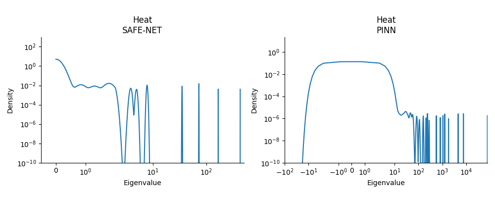
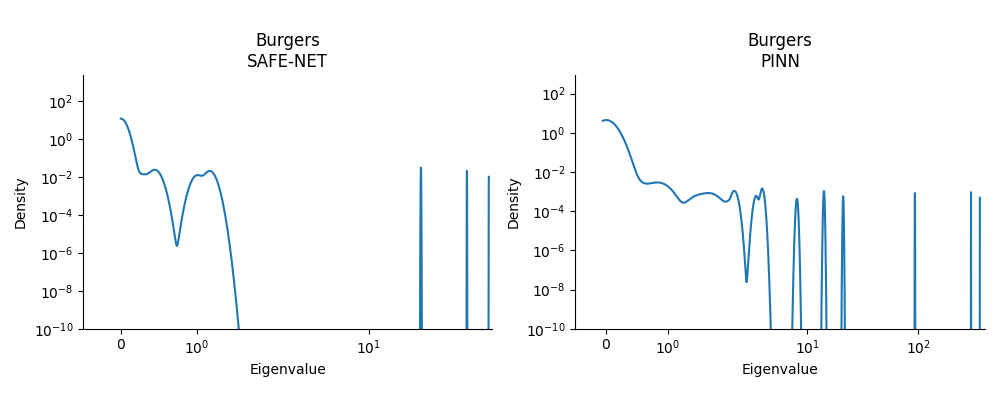
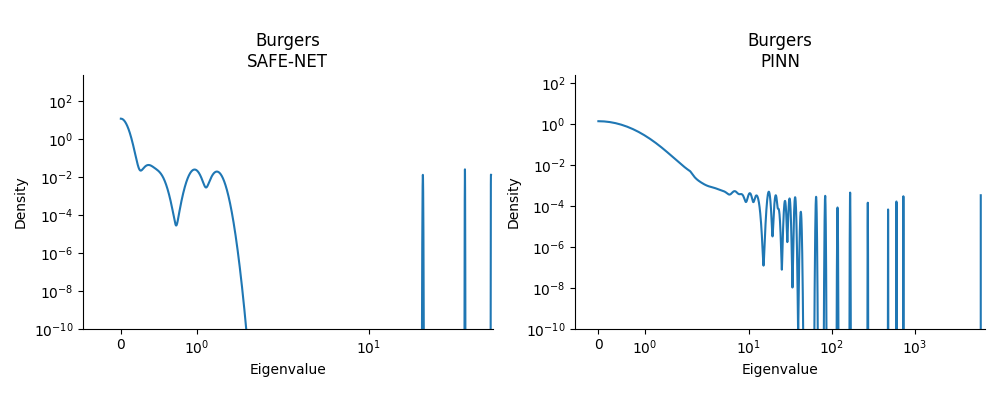
Considerable improvement in the conditioning of the problems even at the initial phase is observed compared to PINN, RFF-PINN, and RBF-PINN, suggesting SAFE-NET’s effectiveness in initialization. Post-training spectral density plots reveal dramatic conditioning improvements: top eigenvalues for the wave and convection problems decrease by a factor of $10^{3}$, while those for the heat and Allen-Cahn problems decrease by $10^{2}$. SAFE-NET reduces both the number and density of large eigenvalues across all problems.

(a)

(b)

Figure 7: Spectral density for the wave PDE using SAFE-NET and PINN at the early stages of training and at the end of training. Similar plots for the feature engineering baseline methods appear in Appendix C for comparison.

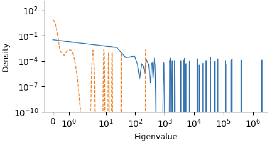
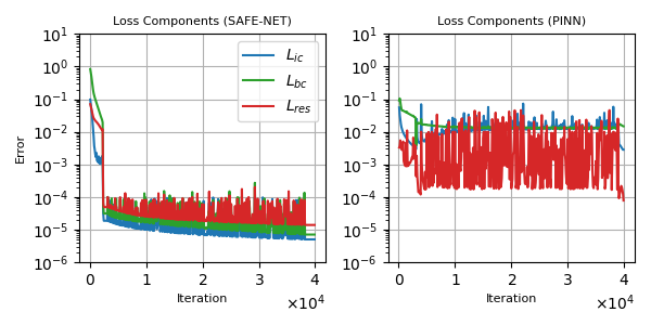
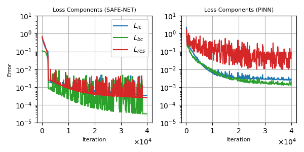
This improvement in conditioning is a key factor explaining why SAFE-NET features are easier to optimize. Figure 8 compares SAFE-NET and PINNs performance on different loss components for the wave and Allen-Cahn PDEs (from the same experiment as Figure 5) as an example. (Rathore et al., 2024) argues the residual loss is the main cause of the ill-conditioned loss landscape of PINNs. SAFE-NET significantly improves the conditioning of each loss component, including the residual loss.

(a)

(b)

Figure 8: Comparison of loss components of Figure 5 with SAFE-NET and PINN with (Adam + L-BFGS)². SAFE-NET significantly improves each loss component for both PDEs.

6 Implicit preconditioning in SAFE-NET

Empirical results in Section 5.3 show SAFE-NET improves the conditioning of each problem both at the beginning and end of training. To develop a better intuition for why this is the case, we consider a simple didactic setting similar to Wang et al. (2020), where the network is given by

$$u(x,t)=w^{\top}\phi(x,t),$$ (9)

here $(x,t)\in\mathbb{R}^{2}$ and $\phi$ is the feature map.

We begin with a definition:

Definition 6.1.

For a neural network $f_{\theta}(x)$ with parameters $\theta\in\mathbb{R}^{p}$, the tangent kernel $\Theta_{f}:\Omega\times\Omega\to\mathbb{R}$ is given by

$$\Theta_{f}(x^{\prime},x)=\nabla_{\theta}f(x)^{\top}\nabla f_{\theta}(x).$$

Given an input dataset $X\in\mathbb{R}^{n\times d}$, the tangent kernel matrix is the $n\times n$ matrix with entries

$$(\Theta_{f}(\theta))_{ij}=\nabla_{\theta}f(x_{i})^{\top}\nabla f_{\theta}(x_{j}),\qquad i,j=1,\ldots,n,$$

where $x_{i}$ and $x_{j}$ are $i$th and $j$th rows of $X$.

The neural tangent kernel $\Theta_{f}^{\infty}\in\mathbb{R}^{n\times n}$ is the fixed kernel defined as

$$\Theta^{\infty}_{f}(x^{\prime},x)=\lim_{p\rightarrow\infty}\mathbb{E}[\Theta_{f}(x^{\prime},x)],$$

where the expectation is taken over the weights at initialization (Jacot et al., 2018; Liu et al., 2020). The neural tangent kernel matrix $\Theta^{\infty}_{f}$ is defined analogously to the tangent kernel matrix.

In the limit $p\rightarrow\infty$, neural net training with $f_{\theta}$ is equivalent to kernel regression with the NTK matrix $\Theta^{\infty}_{f}$. As training is reduced to a kernel regression problem, the convergence speed of gradient-based optimizers is controlled by the conditioning of the NTK matrix $\Theta^{\infty}_{f}$ (Jacot et al., 2018; Liu et al., 2022). Thus, a better-conditioned NTK yields a better optimization landscape and faster convergence.

In the context of (9), we shall argue that the SAFE-NET features lead to a better conditioned NTK and, so, a better optimization landscape. When $n$ and $p$ are large, the spectrum of $\Theta^{\infty}_{f}$ is closely related to the spectrum of the integral operator $T_{\Theta_{f}}(g)(x)\coloneqq\int_{\Omega}\Theta_{f}(x^{\prime},x)g(x)dx.$ (Wang et al., 2020). Thus, we shall obtain control over the $T_{\Theta_{f}}$ spectrum for $f$ given by (9).

We begin by writing the tangent kernel function corresponding to (9). As $\theta=w$, $\nabla_{\theta}u(x,t)=\phi(x,t)$, therefore the tangent kernel function is given by

$$\Theta_{u}\left((x,t),(x^{\prime},t^{\prime})\right)=\phi(x,t)^{\top}\phi(x^{\prime},t^{\prime}).$$

Let us focus on the Fourier basis features. Using the notation of Section 3.2, we have

$$\phi(x,t)=\sum_{i=1}^{N}\sum_{j=1}^{4}c_{j}^{(i)}\phi_{j}^{(i)}(x,t),$$

where $\{\phi_{j}^{(i)}\}_{j=1}^{4}$ are defined in equations (3)-(6) and $i=1,...,N$ are the number of each type of product features. The kernel is a sum of separable functions as

$$\Theta_{u}((x,t),(x^{\prime},t^{\prime}))=\sum_{i=1}^{N}\sum_{j=1}^{4}\big{(}c_{j}^{(i)}\big{)}^{2}\phi_{j}^{(i)}(x,t)\phi_{j}^{(i)}(x^{\prime},t^{\prime}).$$ (10)

The eigenvalues $\beta$ and eigenfunctions $\psi(x,t)$ satisfy

$$\int\Theta_{u}((x,t),(x^{\prime},t^{\prime}))\psi(x^{\prime},t^{\prime})\,dx^{\prime}dt^{\prime}=\beta\psi(x,t).$$

Substituting $\Theta_{n}((x,t),(x^{\prime},t^{\prime}))$ from equation (10), we get

$$\sum_{i=1}^{N}\sum_{j=1}^{4}\big{(}c_{j}^{(i)}\big{)}^{2}\phi_{j}^{(i)}(x,t)\int\phi_{j}^{(i)}(x^{\prime},t^{\prime})\psi(x^{\prime},t^{\prime})=\beta\psi(x,t).$$ (11)

Set $\alpha_{j}^{(i)}:=\int\phi_{j}^{(i)}(x^{\prime},t^{\prime})\psi(x^{\prime},t^{\prime})dx^{\prime}dt^{\prime}$ by the domain compactness assumption, so for $\beta\neq 0$, we get

$$\psi(x,t)=\frac{1}{\beta}\sum_{i=1}^{N}\sum_{j=1}^{4}\alpha_{j}^{(i)}\big{(}c_{j}^{(i)}\big{)}^{2}\phi_{j}^{(i)}(x,t).$$ (12)

To calculate the eigenvalues, substitute equation (12) into equation (11) to get

$$\frac{1}{\beta}\sum_{i,\ell}^{N}\sum_{j,m}^{4}\big{(}c_{j}^{(i)}\big{)}^{2}\phi_{j}^{(i)}\alpha_{m}^{(\ell)}\big{(}c_{m}^{(\ell)}\big{)}^{2}\int\phi_{j}^{(i)}(x^{\prime},t^{\prime})\phi_{m}^{(\ell)}(x^{\prime},t^{\prime})$$

$$=\beta\big{(}\frac{1}{\beta}\sum_{i=1}^{N}\sum_{j=1}^{4}\alpha_{j}^{(i)}\big{(}c_{j}^{(i)}\big{)}^{2}\phi_{j}^{(i)}\big{)}$$

Now, $\{\phi_{j}^{(i)}\}$ forms an orthonormal basis, as each $\phi$ is chosen from an orthogonal Fourier basis and has unit norm. Thus,

$$\frac{1}{\beta}\sum_{i=1}^{N}\sum_{j=1}^{4}\alpha_{j}^{(i)}\big{(}c_{j}^{(i)}\big{)}^{4}\phi_{j}^{(i)}=\sum_{i=1}^{N}\sum_{j=1}^{4}\alpha_{j}^{(i)}\big{(}c_{j}^{(i)}\big{)}^{2}\phi_{j}^{(i)}.$$

From this display, we conclude that for each pair $(i,j)$, $\alpha_{j}^{(i)}\left(c_{j}^{(i)}\right)^{2}=0\quad\text{or}\quad\beta=\left(c_{j}^{(i)}\right)^{2}.$ Thus, the eigenvalues of $T_{\Theta_{u}}$ are $0$ or equal $(c_{j}^{(i)})^{2}$ with corresponding eigenfunction $\psi(x,t)=\alpha_{j}^{(i)}\phi_{j}^{(i)}(x,t)$. As the non-zero eigenvalues correspond to the directions relevant to learning, we focus on them. Recall the $\{c_{j}^{(i)}\}$ are the trainable amplitudes and are set to $1$ at initialization. Hence, at initialization, we expect the condition number of the matrix $\Theta_{u}$ to be approximately 1. If $u$ were in the infinite width limit, this would imply $\Theta^{\infty}_{u}$ is well-conditioned and fast convergence of gradient-based optimizers. Thus, this idealized example shows the features selected by SAFE-NET can lead to better conditioning and faster convergence. In practice, finite network width and perturbations from domain knowledge features and normalization are expected to introduce some spreading in the eigenvalue distribution. However, experiments show that SAFE-NET maintains a denser eigenvalue distribution around the theoretical prediction from the example (see Figure 7(a)), preserving the core conditioning benefits anticipated by the idealized example and its insights. Early on in training, Figure 7 shows the eigenvalue distribution is relatively uniform. During training, SAFE-NET gradually adjusts the $c_{j}^{(i)}$’s, balancing different frequencies rather than letting any single Fourier mode dominate. As a result, the eigenvalue distribution shifts outwards relatively slowly. Thus, even at the end of the training, Figure 7 shows the eigenvalue distribution has not changed much from its initialization, so the landscape remains well-conditioned.

7 Discussion and Future Work

Our results encourage a fresh look at the importance of feature engineering for PDEs. While machine learning trends have favored complex architectures, our work suggests that engineered features can offer a useful implicit bias that deep architectures struggle to replicate. PDEs present unique challenges, including ill-conditioned solution spaces, where deep learning techniques tend to struggle. While newer architectures could offer improvements, our theory shows engineered features can always improve problem conditioning. Hence we expect feature engineering will have lasting importance for solving PDEs, complementing advances in deep learning.

While SAFE-NET demonstrates significant improvements in conditioning and convergence for smooth PDEs, several avenues remain to improve feature engineering in PINNs. The first is Multi-stage feature learning, following (Wang & Lai, 2023), a multi-stage approach that further boosts performance by iteratively learning a best fit on the residual error, using SAFE-NET as a base learner could be developed. Another direction is better incorporating physical priors. Enforcing physical laws such as conservation principles and symmetries into the feature engineering process could improve the performance of SAFE-NET on complex problems. Features based on concepts like Noether’s theorem or Hamiltonian mechanics could provide stronger inductive biases. Finally, it would be interesting to also consider non-Fourier features like radial basis functions for handling sharp gradients, which could allow SAFE-NET to perform well on a wider range of problems. The challenge here lies in maintaining numerical stability when combining these different types of features.

Impact Statement

This paper presents work whose goal is to advance the field of scientific machine learning. There are many potential societal consequences of our work, none which we feel must be specifically highlighted here.

Appendix

Appendix A Additional Experimental Setup Details

A.1 Physics-informed Neural Networks

Physics-Informed Neural Networks (PINNs) are a class of neural networks that incorporate physical laws described by Partial Differential Equations (PDEs) into the training process. PINNs solve forward and inverse problems involving PDEs by embedding the physics constraints into the loss function. They aim to solve PDE systems of the form:

$$D[u(x),x]=0,\quad x\in\Omega$$

$$B[u(x),x]=0,\quad x\in\partial\Omega$$

$$I[u(x),x]=0,\quad x\in\Omega$$

Where $D$ represents the differential operator defining the PDE, $B$ represents the boundary conditions. $I$ represents the initial conditions, important for time-dependent problems, and $\Omega\subseteq\mathbb{R}^{d}$ is the domain of the PDE.

Loss Function in PINNs. PINNs minimize a non-linear least-squares loss consisting of three terms:

$$L(w)=\frac{1}{2n_{\text{res}}}\sum_{i=1}^{n_{\text{res}}}\left(D[u(x_{i}^{r};w),x_{i}^{r}]\right)^{2}+\frac{1}{2n_{\text{bc}}}\sum_{j=1}^{n_{\text{bc}}}\left(B[u(x_{j}^{b};w),x_{j}^{b}]\right)^{2}+\frac{1}{2n_{\text{ic}}}\sum_{k=1}^{n_{\text{ic}}}\left(I[u(x_{k}^{i};w),x_{k}^{i}]\right)^{2}$$

here the first term $(D)$ represents the PDE residual loss, the second term $(B)$ represents the boundary condition loss, and the third term $(I)$ ensures the initial condition loss for time-dependent problems.

$L^{2}$ Relative Error. In each setup, the discrepancy between the predicted solution and the ground truth is evaluated using the $\ell_{2}$ relative error (L2RE), a standard metric in the PINN literature. Given the PINN prediction $\mathbf{y}=(y_{i})_{i=1}^{n}$ and the ground truth $\mathbf{y^{\prime}}=(y^{\prime}_{i})_{i=1}^{n}$, the L2RE is defined as:

$$L2RE=\sqrt{\frac{\sum_{i=1}^{n}(y_{i}-y^{\prime}_{i})^{2}}{\sum_{i=1}^{n}(y^{\prime}_{i})^{2}}}=\frac{\|\mathbf{y}-\mathbf{y^{\prime}}\|_{2}}{\|\mathbf{y^{\prime}}\|_{2}}.$$

A.2 SAFE-NET’s Setup

In this section, we provide a detailed description of SAFE-NET’s architecture, including its network structure, parameter initialization, normalization techniques, and a step-by-step explanation of its operation. SAFE-NET is designed to solve partial differential equations (PDEs) by incorporating trainable feature mappings and domain-specific knowledge into a neural network framework.

A.2.1 Network Architecture

SAFE-NET consists of two main components: a Feature Generator and an MLP. The architecture is configured as follows:

• Number of Layers: 1 hidden layer.

• Number of Neurons per Layer: 50 neurons in the hidden layer.

• Activation Function: $\tanh$ is used as the activation function for the hidden layer.

• Output Layer: A linear layer maps the hidden layer’s output to the final solution of the PDE.

A.2.2 Feature Generator

The Feature Generator is responsible for creating enriched input features by combining Fourier-based cross terms and domain-specific features. It is defined as follows:

• Fourier Cross Terms: Four sets of trainable Fourier features are generated using sine and cosine functions with trainable frequencies and coefficients:

  $$\sum_{i}\text{coeff}_{1}[i]\cdot\sin(\omega_{x}[i]\cdot x)\cdot\cos(\omega_{t}[i]\cdot t),$$

  $$\sum_{i}\text{coeff}_{2}[i]\cdot\sin(\omega_{t}[i]\cdot t)\cdot\cos(\omega_{x}[i]\cdot x),$$

  $$\sum_{i}\text{coeff}_{3}[i]\cdot\sin(\omega_{x}[i]\cdot x)\cdot\sin(\omega_{t}[i]\cdot t),$$

  $$\sum_{i}\text{coeff}_{4}[i]\cdot\cos(\omega_{x}[i]\cdot x)\cdot\cos(\omega_{t}[i]\cdot t).$$

  Here, $\omega_{x}$ and $\omega_{t}$ are trainable frequencies, and the coefficients are also trainable parameters.

• Domain-Specific Features: Depending on the PDE type (e.g., wave, convection, heat, etc.), additional features are incorporated based on the initial and boundary conditions to leverage domain knowledge. For example:

  • For the wave equation, features include $\sin(\pi x)$, $\sin(5\pi x)$, and their linear combinations.

  • For the heat equation, features include $x^{2}$, $2-x$, and their products.

  • For the convection equation and the Burgers equation, $\sin(x)$ and $-\sin(x)$ are used respectively.

  • For the diffusion equation, Gaussian features such as $h(x)=\exp\left(-\frac{(x-\pi)^{2}}{2(\pi/4)^{2}}\right)$ are incorporated.

  • For the NS equation, features include $y$, $1-y$, and their products.

A.2.3 Normalization

The generated features are normalized using a centered $L_{2}$ normalization technique:

1. Centering: The mean of the features is subtracted to center the data.

2. Normalization: The centered features are divided by their $L_{2}$ norm to ensure numerical stability and consistent scaling.

Mathematically, the normalization is defined as:

$$v_{\text{normalized}}=\frac{v-\text{mean}(v)}{\|v-\text{mean}(v)\|_{2}+\epsilon},$$

where $\epsilon=10^{-3}$ is a small constant to avoid division by zero.

A.2.4 Parameter Initialization

• Fourier Frequencies: Initialized as $\omega_{x}=\omega_{t}=[\pi,2\pi,\dots,n\pi]$, where $n$ is the number of cross features. This initialization is aligned with the orthogonal Fourier basis terms in the Fourier series approximating the solution.

• Fourier Coefficients: Initialized to 1 for all terms.

• MLP Weights: Initialized using PyTorch’s default initialization scheme.

A.3 Baseline Methods’ Setups

For all the PINN-based baseline methods, we used 4 layers with 50 neurons per layer and the $\tanh$ activation function. In addition, for each of the feature engineering baseline methods, we used 128 features–same as the number used in their respective papers. For fair comparison, we also used 128 features for SAFE-NET in our experiments, unless stated otherwise. We now provide a quick summary of each method used and any other specific setup details not stated in the general instructions above.

A.3.1 W-PINN

From (Wang et al., 2022), W-PINN (Weighted Physics-Informed Neural Network) is a variant of PINN that addresses spectral bias and imbalanced convergence rates in multi-term loss functions through adaptive weight calibration. For a PDE defined as:

$$\mathcal{L}u=f(\bm{x}),\ \bm{x}\in\Omega\quad\text{with boundary conditions }\ u(\bm{x})=g(\bm{x}),\ \bm{x}\in\partial\Omega$$ (13)

W-PINN builds upon the observation that for a PINN model solving a PDE, the total loss function typically takes the form:

$$\mathcal{L}(\theta)=\lambda_{b}\mathcal{L}_{b}(\theta)+\lambda_{r}\mathcal{L}_{r}(\theta)$$ (14)

where $\mathcal{L}_{b}$ represents the boundary condition loss, $\mathcal{L}_{r}$ denotes the PDE residual loss, and $\lambda_{b},\lambda_{r}$ are their respective weights. The gradient flow dynamics of this system can be expressed as:

$$\begin{bmatrix}\frac{du(x_{b},\theta(t))}{dt}\\ \frac{d\mathcal{L}u(x_{r},\theta(t))}{dt}\end{bmatrix}=-\begin{bmatrix}\frac{\lambda_{b}}{N_{b}}\mathbf{K}_{uu}(t)&\frac{\lambda_{r}}{N_{r}}\mathbf{K}_{ur}(t)\\ \frac{\lambda_{b}}{N_{b}}\mathbf{K}_{ru}(t)&\frac{\lambda_{r}}{N_{r}}\mathbf{K}_{rr}(t)\end{bmatrix}\begin{bmatrix}u(x_{b},\theta(t))-g(x_{b})\\ \mathcal{L}u(x_{r},\theta(t))-f(x_{r})\end{bmatrix}$$ (15)

We refer the reader to (Wang et al., 2021b) for details of these calculations and definitions. The key insight of w-PINN is that the eigenvalues of the NTK matrices $\mathbf{K}_{uu}$ and $\mathbf{K}_{rr}$ characterize the convergence rates of the boundary and residual losses respectively. The method proposes adapting the weights according to:

$$\lambda_{b}=\frac{\text{Tr}(\mathbf{K})}{\text{Tr}(\mathbf{K}_{uu})}$$ (16)

$$\lambda_{r}=\frac{\text{Tr}(\mathbf{K})}{\text{Tr}(\mathbf{K}_{rr})}$$ (17)

where $\text{Tr}(\cdot)$ denotes the matrix trace operator and $\mathbf{K}$ is the full NTK matrix.

A.3.2 A-PINN

The Adaptive Physics-Informed Neural Network (A-PINN) from (Jagtap et al., 2020) introduces a dynamic approach to improve the training and accuracy of PINNs by incorporating adaptable activation functions. Consider a neural network of depth $D$ with an input layer, $D-1$ hidden layers, and an output layer. For the $k$-th hidden layer containing $N_{k}$ neurons, the network receives output $z^{k-1}\in\mathbb{R}^{N_{k-1}}$ from the previous layer. The affine transformation in each layer takes the form:

$$L_{k}(z^{k-1}):=w^{k}z^{k-1}+b^{k}$$ (18)

where $w^{k}\in\mathbb{R}^{N_{k}\times N_{k-1}}$ represents the weights and $b^{k}\in\mathbb{R}^{N_{k}}$ represents the bias terms. A-PINN introduces a trainable scaling parameter $a$ in the activation function:

$$\sigma(naL_{k}(z^{k-1}))$$ (19)

where:

• $a$ is an adaptable hyper-parameter that needs to be optimized

• $n\geq 1$ is a scaling factor that accelerates convergence

• $\sigma(\cdot)$ is any standard activation function ($\tanh$, ReLU, etc.).

(Jagtap et al., 2020) uses different values of $n$ for their tests, and while there is little explanation on why certain numerical values are better, they determine that $n=5$ or $n=10$ work well for their tested PDEs, so we use $n=10$ as well in our comparison. Also, we chose the best performing activation function for this method, the $\tanh$ function, in our experiments.

A.3.3 RFF-PINN

The Random Fourier Feature PINN (RFF-PINN) builds upon the theoretical foundations of NTK theory by using random Fourier feature mappings as coordinate embeddings before the input layer of the neural network. The random Fourier mapping $\gamma$ is defined as:

$$\gamma(v)=\begin{pmatrix}\cos(Bv)\\ \sin(Bv)\end{pmatrix}$$ (20)

where $B\in\mathbb{R}^{m\times d}$ contains entries sampled from a Gaussian distribution $\mathcal{N}(0,\sigma^{2})$, and $\sigma>0$ is a user-specified hyperparameter that controls the frequency scale of the features. The complete RFF-PINN architecture consists of:

1. A random Fourier feature mapping layer that transforms input coordinates

2. A conventional fully-connected neural network that processes the transformed inputs

3. Output layers that produce the solution

The paper demonstrates that the choice of $\sigma$ is problem-dependent and should be selected based on the expected frequency characteristics of the solution. Notably, they suggest that when dealing with high-frequency spatial variations, using larger $\sigma$ values (like 200) can be beneficial, while for temporal variations or smoother spatial variations, smaller values (like 1 or 10) are often sufficient. In our experiments, we adopt the same strategy by taking $\sigma$ = 200 for the spatial coordinates and $\sigma$ = 10 for the temporal coordinate (if the PDE is time-dependent). Experiments with other values did not lead to improved results.

A.3.4 RBF-PINN

RBF-PINN (Radial Basis Functions PINN) from (Zeng et al., 2024b) uses non-Fourier positional embedding to enhance the network’s ability to learn multi-scale features. RBF-PINN is motivated by insights from NTK theory, which shows that the continuous approximation of a neural network function can be analyzed through the convolution of a stationary composed NTK function:

$$K_{COMP}(x)=(K_{COMP}*\delta_{x})(x)=\int K_{COMP}(x^{\prime})K_{\Phi}(x-x^{\prime})dx$$ (21)

The accuracy of this approximation can be analyzed through Taylor series expansion:

$$\begin{split}K_{COMP}(x)=\int(&K_{COMP}(x)+\nabla_{x}K_{COMP}(x-x^{\prime})+\\ &\frac{1}{2}(x-x^{\prime})\nabla^{2}K_{COMP}(x-x^{\prime})+O((x-x^{\prime})^{3}))K_{\Phi}(x-x^{\prime})dx\end{split}$$ (22)

The feature mapping function is defined as:

$$\Phi(x)=\frac{\sum_{i}^{m}w_{i}\phi(|x-c_{i}|)}{\sum_{i}^{m}\phi(|x-c_{i}|)}$$ (23)

where:

• $x\in\mathbb{R}^{n}$ is the input data

• $c\in\mathbb{R}^{n\times m}$ are the centers of the RBFs (trainable parameters)

• $w$ is the weight matrix for the feature mapping layer

For practical implementation, the following considerations are made:

• The RBF feature mapping layer uses 128 RBFs by default, as this provides a good balance between performance and computational efficiency.

• The RBFs are initialized with centers $c_{i}$ sampled from a standard Gaussian distribution, and the bandwidth of the RBFs is controlled by the compact support radius $\xi$. The performance of RBF-PINN is highly dependent on the choice of kernel hyperparameters, particularly the compact support radius $\xi$ and the bandwidth of the RBFs. Below, we describe the tuning process used in our experiments:

  • Compact Support Radius ($\xi$):

    • The compact support radius $\xi$ controls the bandwidth of the RBFs. A smaller $\xi$ results in a narrower kernel, which is better suited for high-frequency problems, while a larger $\xi$ is more appropriate for low-frequency problems.

    • We tuned $\xi$ using a grid search over a range of values $\xi\in[0.1,2.0]$) and selected the value that minimized the validation error for each specific problem. For example, in the Diffusion equation, a smaller $\xi$ of $0.5$ was found to be optimal, while for the Wave equation, a larger $\xi$ ($\xi=2$) performed better.

  • Bandwidth of RBFs:

    • The bandwidth of the RBFs is controlled by the standard deviation $\sigma$ of the Gaussian RBFs. We used the Gaussian RBF formulation:

      $$\phi(r)=e^{-\frac{r^{2}}{\sigma^{2}}},$$

      where $r=\|x-c_{i}\|$ is the Euclidean distance between the input $x$ and the RBF center $c_{i}$.

    • The bandwidth $\sigma$ was tuned using a similar grid search approach for $\sigma\in[0.1,2.0]$.

• For certain problems, RBF-PINN can be enhanced by adding polynomial terms to the feature mapping layer. In our experiments, we used 10 polynomial terms unless otherwise specified, as this was found to provide a good trade-off between expressivity and computational overhead.

The loss function maintains the standard PINN structure.

A.4 Optimizers

In this section, we detail the optimizers used in our experiments and the rationale behind their selection. For the general comparison involving SAFE-NET and baseline methods, we employ the Adam optimizer, as it is the primary optimizer used in the referenced works for the majority of these methods. For these experiments, we run Adam for 150,000 training epochs with an initial learning rate of 0.001. A decay factor of 0.9 is applied every 2,000 epochs toward the end of training, starting in the last 20,000 iterations.

For the remaining experiments with SAFE-NET, we utilize an adaptive combination of Adam and L-BFGS, referred to as (Adam + L-BFGS)², trained for 40,000 epochs. This approach is specifically employed to demonstrate SAFE-NET’s performance and compatibility with L-BFGS and its ability to leverage the strengths of both optimizers. The (Adam + L-BFGS)² approach runs 3000 Adam iterations, switches to L-BFGS until convergence stalls, reverts to Adam, and finally switches back to L-BFGS for the last 3000 epochs. For this approach, Adam’s learning rate is set to be 0.001, and for L-BFGS, we use a default learning rate of 1.0, a memory size of 100, and employ a strong Wolfe line search.

Motivation behind the choice of (Adam + L-BFGS)². L-BFGS is widely recognized as an effective optimizer for PINNs and their variants. However, it is often observed that L-BFGS stalls prematurely, failing to reach the maximum number of iterations. For a detailed analysis of why Adam + L-BFGS outperforms Adam or L-BFGS alone, we refer the reader to (Rathore et al., 2024).

To identify the optimal combination of Adam and L-BFGS for SAFE-NET, we tested various configurations. Our experiments revealed that, for the PDEs studied in this work, L-BFGS provides significant improvement during its initial application but stalls before completing 3,000 epochs. Subsequent uses of L-BFGS in the combined optimizer yield negligible improvements and also stall quickly. Additionally, employing L-BFGS before Adam risks divergence or convergence to saddle points (see (Rathore et al., 2024) for further discussion).

Based on these observations, we employ L-BFGS twice: once after an initial 3,000 epochs of Adam until convergence stalls, and again at the end of training for another 3,000 epochs. While the second application of L-BFGS typically provides minimal improvement and stalls early, we designed (Adam + L-BFGS)² to adaptively switch to Adam when L-BFGS stalls during its first phase, avoiding wasted epochs. In the accompanying figures, we demonstrate SAFE-NET’s performance on the wave PDE using different combinations of Adam and L-BFGS. These results validate that (Adam + L-BFGS)² achieves superior performance, confirming the effectiveness of our chosen hyperparameters.

(a)

(b)

(c)

(d)

Figure 9: Hyperparameter analysis results for combinations of Adam and L-BFGS using SAFE-NET on the wave PDE. L-BFGS stalls quickly no matter which epoch it starts at, and the significant improvement occurs only in the first round of L-BFGS. Running Adam again after L-BFGS gives us the most efficient combination

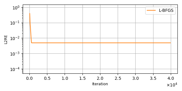
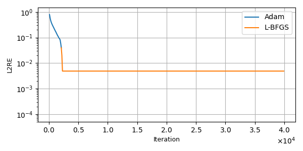
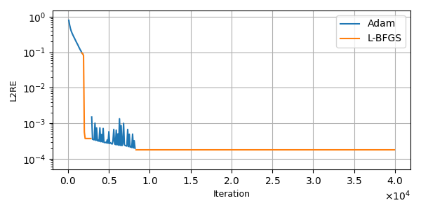
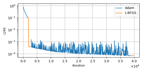
(Adam + L-BFGS)² is unsuitable for general comparisons with the baseline methods. Our experiments demonstrate that (Adam + L-BFGS)² is not a suitable optimizer for general comparisons with all baseline methods. This is primarily due to the tendency of L-BFGS to induce divergence or instability in other PINN variants, particularly in problems with specific PDE characteristics or architectural choices, such as certain feature mapping functions. Additionally, L-BFGS often diverges due to numerical instability, a issue exacerbated when specialized features are introduced into the network. Although Adam + L-BFGS is commonly used in PINN setups, we observe that (Adam + L-BFGS)² fails to improve—and often degrades—performance for most baseline methods across various problems, rendering it unsuitable for general comparison experiments. Specifically, the second Adam phase following the first round of L-BFGS either fails to improve or worsens the loss in most cases for other baseline methods.

To ensure a fair comparison, we do not employ (Adam + L-BFGS)² as the primary optimizer for our main experiments. However, for completeness, we provide Table 5, which summarizes the numerical results obtained for each PDE using (Adam + L-BFGS)² with all baseline methods. The symbol $\times$ indicates cases where L-BFGS diverges and fails to produce valid numerical results. Notably, SAFE-NET exhibits robust performance under (Adam + L-BFGS)², highlighting its unique compatibility with this optimizer. This further underscores the adaptability of SAFE-NET compared to other baseline methods.

Table 5: Numerical results for several PDEs using the baseline methods and (Adam + L-BFGS)²

PDE	PINN	A-PINN	W-PINN
Wave	$3.17\text{e}{-2}$	$2.43\text{e}{-2}$	$4.13\text{e}{-2}$
Diffusion	$1.43\text{e}{-3}$	$2.65\text{e}{-4}$	$2.36\text{e}{-4}$
Heat	$\times$	$\times$	$\times$
Convection	$4.21\text{e}{-3}$	$\times$	$6.61\text{e}{-4}$
Allen-Cahn	$\times$	$3.31\text{e}{-2}$	$\times$
Burgers	$1.34\text{e}{-2}$	$\times$	$6.37\text{e}{-2}$
NS (Re=1000)	$4.49\text{e}{-1}$	$1.15\text{e}{-1}$	$1.87\text{e}{-1}$
PDE	RBF-PINN	RFF-PINN	SAFE-NET
Wave	$3.78\text{e}{-2}$	$4.41\text{e}{-4}$	$\boldsymbol{7.05\text{e}{-5}}$
Diffusion	${7.81\text{e}{-4}}$	$\times$	$\boldsymbol{6.13\text{e}{-4}}$
Heat	$6.51\text{e}{-5}$	$2.63\text{e}{-4}$	$\boldsymbol{4.93\text{e}{-6}}$
Convection	$\times$	$\times$	$\boldsymbol{6.26\text{e}{-5}}$
Allen-Cahn	$5.63\text{e}{-1}$	$1.35\text{e}{-2}$	$\boldsymbol{3.61\text{e}{-4}}$
Burgers	$\boldsymbol{2.43\text{e}{-5}}$	$\times$	$6.97\text{e}{-5}$
NS (Re=1000)	${2.73\text{e}{-1}}$	$3.43\text{e}{-1}$	$\boldsymbol{8.73\text{e}{-2}}$

Appendix B Additional Details on the Tested PDEs

In this section of the appendix, we present the differential equations we study in our experiments.

B.1 Wave

The wave equation, a type of hyperbolic partial differential equation (PDE), is commonly encountered in the study of phenomena such as acoustics, electromagnetism, and fluid dynamics. Our focus is on the following wave equation:

$$\frac{\partial^{2}u}{\partial t^{2}}-4\frac{\partial^{2}u}{\partial x^{2}}=0,\quad x\in(0,1),\ t\in(0,1),$$

with the initial conditions:

$$u(x,0)=\sin(\pi x)+\frac{1}{2}\sin(5\pi x),\quad x\in[0,1],$$

$$\frac{\partial u(x,0)}{\partial t}=0,\quad x\in[0,1],$$

and boundary conditions:

$$u(0,t)=u(1,t)=0,\quad t\in[0,1].$$

The analytical solution for this PDE, setting $\beta=5$, is given by $u(x,t)=\sin(\pi x)\cos(2\pi t)+\frac{1}{2}\sin(5\pi x)\cos(10\pi t)$.

B.2 Convection

The convection equation, another hyperbolic PDE, models processes such as fluid flow, heat transfer, and biological dynamics. We examine this equation:

$$\frac{\partial u}{\partial t}+\beta\frac{\partial u}{\partial x}=0,\quad x\in(0,2\pi),\ t\in(0,1),$$

with the initial condition:

$$u(x,0)=\sin(x),\quad xin[0,2\pi],$$

and the cyclic boundary condition:

$$u(0,t)=u(2\pi,t),\quad t\in[0,1].$$

The exact solution to this equation with $\beta=40$ is $u(x,t)=\sin(x-40t)$.

B.3 Heat

The heat equation is fundamental in the mathematical modeling of thermal diffusion processes. It is widely applied in fields such as thermodynamics, material science, and environmental engineering to analyze heat distribution over time within solid objects. This equation is also crucial in understanding temperature variations in earth sciences, predicting weather patterns in meteorology, and simulating cooling processes in manufacturing industries. We study this parabolic PDE, expressed as:

$$\frac{\partial u}{\partial t}-4\frac{\partial^{2}u}{\partial x^{2}}=0,\quad x\in[0,2],\ t\in[0,0.2],$$

with the initial profile:

$$u(x,0)=x^{2}(2-x),\quad x\in[0,2],$$

and fixed boundary conditions:

$$u(0,t)=u(2,t)=0,\quad t\in[0,0.2].$$

The experiments use $\kappa=2$.

B.4 Burgers

The Burgers equation, a fundamental partial differential equation (PDE) in fluid mechanics, is used to model various nonlinear phenomena including shock waves and traffic flow. We examine the following form of the Burgers’ equation:

$$\frac{\partial u}{\partial t}+u\frac{\partial u}{\partial x}=\nu\frac{\partial^{2}u}{\partial x^{2}},\quad x\in[-1,1],\ t\in[0,1],$$

where $\nu=\frac{0.01}{\pi}$ represents the viscosity, crucial for modeling the diffusion effects.

The boundary conditions are periodic:

$$u(-1,t)=u(1,t)=0,\quad t\in[0,1],$$

and the initial condition is given by:

$$u(x,0)=-\sin(\pi x),\quad x\in[-1,1].$$

The analytical solution to this PDE, which can be derived under certain conditions, represents the evolution of the wave profile influenced by both convection and diffusion. This equation helps illustrate the balance between nonlinear advection and viscosity, essential for understanding the dynamics of the modeled system.

B.5 Diffusion

The diffusion equation, a nonlinear ordinary differential equation (ODE), is useful for modeling chemical kinetics. We analyze it under the conditions:

$$\frac{\partial u}{\partial t}-5u(1-u)=0,\quad x\in(0,2\pi),\ t\in(0,1),$$

$$u(x,0)=\exp\left(-\frac{(x-\pi)^{2}}{2(\pi/4)^{2}}\right),\quad x\in[0,2\pi],$$

$$u(0,t)=u(2\pi,t),\quad t\in[0,1].$$

The solution formula for this ODE with $\rho=5$ is expressed as $u(x,t)=\frac{h(x)e^{5t}}{h(x)e^{5t}+1-h(x)}$, where $h(x)=\exp\left(-\frac{(x-\pi)^{2}}{2(\pi/4)^{2}}\right)$.

B.6 Allen-Cahn

The steady-state Allen-Cahn equation is a fundamental partial differential equation (PDE) used in the study of phase separation and transition phenomena. We examine the following form of the 2D steady-state Allen-Cahn equation:

$$\epsilon^{2}\left(\frac{\partial^{2}u}{\partial x^{2}}+\frac{\partial^{2}u}{\partial y^{2}}\right)+u-u^{3}=0,\quad x,y\in[0,2\pi],$$

where $\epsilon$ is a positive constant representing the interface width, which we set to be equal to 1 in our experiments.

The boundary conditions are periodic:

$$u(0,y)=u(2\pi,y),\quad u(x,0)=u(x,2\pi).$$

The analytical solution to this PDE, which can be derived under certain conditions, represents the equilibrium state of the phase field influenced by diffusion and the nonlinear potential. This equation helps illustrate the steady-state behavior of phase separation and is essential for understanding the equilibrium properties of the modeled system.

B.7 Lid-driven Cavity Flow (Navier-Stokes)

The steady incompressible Navier-Stokes equations are given by:

$$\nabla\cdot\mathbf{u}=0,$$

$$\mathbf{u}\cdot\nabla\mathbf{u}+\nabla p-\frac{1}{Re}\Delta\mathbf{u}=0.$$

In the domain (back step flow) of:

$$\mathbf{x}\in\Omega=[0,4]\times[0,2]\setminus([0,2]\times[1,2]\cup R_{i}),$$

where:

• $\mathbf{u}=(u_{x},u_{y})$ is the velocity vector,

• $p$ is the pressure,

• $Re=1000$ is the Reynolds number.

Boundary conditions are give by:

• No-slip condition: $\mathbf{u}=0$,

• Inlet: $u_{x}=4y(1-y),\quad u_{y}=0$,

• Outlet: $p=0$.

These equations describe the steady-state flow of an incompressible fluid, balancing the effects of inertia, pressure, and viscosity. The boundary conditions specify the flow behavior at the domain boundaries, essential for modeling the back step flow scenario.

Appendix C Additional Experimental Remarks

C.1 Complete Results for Figure 7

For details of how to calculate spectral density of the hessian, see Appendix C of (Rathore et al., 2024). Figures 11(a), 12(a), 13(a), and 14(a) display the spectral density plots at the early stages of training for the wave, convection, heat, Burgers, and reaction problems respectively, indicating considerable improvements in the conditioning of the problems even at this initial phase, which suggests that SAFE-NET possesses a more efficient and better initialization as well. Additionally, Figures 11(b), 12(b), 13(b), and 14(b) present the spectral density plots at the end of the training period for each of these problems. Again, we observe dramatic improvements in the conditioning of each problem using SAFE-NET. In particular, the top eigenvalues for the wave and convection problems are reduced by a factor of $10^{3}$, the top eigenvalues for the heat and Burgers problems are reduced by a factor of $10^{2}$. Overall, we observe a significant reduction in the number and density of large eigenvalues in each problem as well.

(a)

(b)

Figure 10: Spectral density plots at the beginning and end of training for the wave PDE with RFF-PINN and RBF-PINN. Comapre with Figure 7 demonstrating spectral density for PINN and SAFE-NET

(a)

(b)

Figure 11: Spectral density plots at the beginning and end of training for the reaction PDE

(a)

(b)

Figure 12: Spectral density plots at the beginning and end of training for the convection PDE

(a)

(b)

Figure 13: Spectral density plots at the beginning and end of training for the heat PDE

(a)

(b)

Figure 14: Spectral density plots at the beginning and end of training for the burgers PDE

C.2 Numerical Results for Figure 6–The Complete Version of Table 4

Here, we present the complete version of Table 6. Our results demonstrate that in most PDEs, the error order of magnitude drops as the number of features increases up to a point, remaining mostly consistent afterwards, suggesting that more features mean more parameters to train, increasing computational cost but potentially negligible improvement in performance.

Table 6: Relative $L^{2}$ errors for different PDEs using SAFE-NET with (Adam + L-BFGS)² using different number of features

# Features	Wave	Diffusion	Heat
16	$1.89\text{e}{-3}$	$4.49\text{e}{-3}$	$7.43\text{e}{-4}$
32	$4.13\text{e}{-4}$	$5.12\text{e}{-3}$	$4.78\text{e}{-5}$
48	$2.17\text{e}{-4}$	$3.93\text{e}{-3}$	$5.48\text{e}{-5}$
64	$1.08\text{e}{-4}$	$4.13\text{e}{-3}$	$2.67\text{e}{-5}$
80	$9.72\text{e}{-5}$	$1.07\text{e}{-3}$	$9.98\text{e}{-6}$
96	$9.21\text{e}{-5}$	$8.62\text{e}{-4}$	$7.62\text{e}{-6}$
112	$8.25\text{e}-5$	$8.81\text{e}{-4}$	$8.48\text{e}{-6}$
128	$7.05\text{e}{-5}$	$6.13\text{e}{-4}$	$4.93\text{e}{-6}$
144	$6.11\text{e}{-5}$	$5.98\text{e}{-4}$	$2.98\text{e}{-6}$
160	$7.19\text{e}{-5}$	$3.21\text{e}{-4}$	$3.17\text{e}{-6}$
192	$7.09\text{e}{-5}$	$4.46\text{e}{-4}$	$2.76\text{e}{-6}$
224	$6.99\text{e}{-5}$	$1.07\text{e}{-4}$	$1.89\text{e}{-6}$
256	$6.86\text{e}{-5}$	$1.24\text{e}{-4}$	$2.10\text{e}{-6}$
Convection	Allen-Cahn	Burgers	NS (Re=1000)
$7.87\text{e}{-3}$	$1.27\text{e}{-2}$	$1.29\text{e}{-3}$	$8.65\text{e}{-1}$
$8.12\text{e}{-4}$	$8.52\text{e}{-3}$	$7.98\text{e}{-4}$	$5.38\text{e}{-1}$
$5.27\text{e}{-4}$	$6.12\text{e}{-3}$	$5.39\text{e}{-4}$	$4.89\text{e}{-1}$
$2.17\text{e}{-4}$	$2.76\text{e}{-3}$	$2.32\text{e}{-4}$	$4.27\text{e}{-1}$
$9.67\text{e}{-5}$	$1.19\text{e}{-3}$	$8.17\text{e}{-5}$	$3.39\text{e}{-1}$
$7.19\text{e}{-5}$	$8.41\text{e}{-4}$	$5.97\text{e}{-5}$	$3.55\text{e}{-1}$
$4.97\text{e}{-5}$	$5.52\text{e}{-4}$	$6.13\text{e}{-5}$	$2.19\text{e}{-1}$
$6.26\text{e}{-5}$	$3.61\text{e}{-4}$	$6.97\text{e}{-5}$	$8.73\text{e}{-2}$
$6.01\text{e}{-5}$	$4.18\text{e}{-4}$	$5.86\text{e}{-5}$	$9.43\text{e}{-2}$
$5.77\text{e}{-5}$	$2.19\text{e}{-4}$	$5.11\text{e}{-5}$	$8.88\text{e}{-2}$
$5.19\text{e}{-5}$	$3.08\text{e}{-4}$	$4.76\text{e}{-5}$	$9.76\text{e}{-2}$
$4.12\text{e}{-5}$	$2.41\text{e}{-4}$	$3.23\text{e}{-5}$	$8.68\text{e}{-2}$
$4.47\text{e}{-5}$	$1.65\text{e}{-4}$	$4.37\text{e}{-5}$	$7.98\text{e}{-2}$

References

- De Ryck et al. (2023) De Ryck, T., Bonnet, F., Mishra, S., and de Bézenac, E. An operator preconditioning perspective on training in physics-informed machine learning. arXiv preprint arXiv:2310.05801, 2023.
- Jacot et al. (2018) Jacot, A., Gabriel, F., and Hongler, C. Neural tangent kernel: Convergence and generalization in neural networks. Advances in neural information processing systems, 31, 2018.
- Jagtap et al. (2020) Jagtap, A. D., Kawaguchi, K., and Karniadakis, G. E. Adaptive activation functions accelerate convergence in deep and physics-informed neural networks. Journal of Computational Physics, 404:109136, 2020.
- Karniadakis et al. (2021) Karniadakis, G. E., Kevrekidis, I. G., Lu, L., Perdikaris, P., Wang, S., and Yang, L. Physics-informed machine learning. Nature Reviews Physics, 3(6):422–440, 2021.
- Kingma & Ba (2014) Kingma, D. P. and Ba, J. Adam: A method for stochastic optimization. arXiv preprint arXiv:1412.6980, 2014.
- Krishnapriyan et al. (2021) Krishnapriyan, A., Gholami, A., Zhe, S., Kirby, R., and Mahoney, M. W. Characterizing possible failure modes in physics-informed neural networks. In Advances in Neural Information Processing Systems, 2021.
- Li et al. (2020a) Li, K., Tang, K., Wu, T., and Liao, Q. D3M: A Deep Domain Decomposition Method for Partial Differential Equations. IEEE Access, 8:5283–5294, 2020a.
- Li et al. (2020b) Li, Z., Kovachki, N., Azizzadenesheli, K., Liu, B., Bhattacharya, K., Stuart, A., and Anandkumar, A. Fourier neural operator for parametric partial differential equations. arXiv preprint arXiv:2010.08895, 2020b.
- Liu et al. (2020) Liu, C., Zhu, L., and Belkin, M. On the linearity of large non-linear models: when and why the tangent kernel is constant. Advances in Neural Information Processing Systems, 2020.
- Liu et al. (2022) Liu, C., Zhu, L., and Belkin, M. Loss landscapes and optimization in over-parameterized non-linear systems and neural networks. Applied and Computational Harmonic Analysis, 59:85–116, 2022.
- Müller & Zeinhofer (2023) Müller, J. and Zeinhofer, M. Achieving High Accuracy with PINNs via Energy Natural Gradient Descent. In Proceedings of the 40th International Conference on Machine Learning, 2023.
- Raissi et al. (2019) Raissi, M., Perdikaris, P., and Karniadakis, G. Physics-informed neural networks: A deep learning framework for solving forward and inverse problems involving nonlinear partial differential equations. Journal of Computational Physics, 378:686–707, 2019.
- Rathore et al. (2024) Rathore, P., Lei, W., Frangella, Z., Lu, L., and Udell, M. Challenges in training PINNs: A loss landscape perspective. In Forty-first International Conference on Machine Learning, 2024.
- Tancik et al. (2020) Tancik, M., Srinivasan, P. P., Mildenhall, B., Fridovich-Keil, S., Raghavan, N., Singhal, U., Ramamoorthi, R., Barron, J. T., and Ng, R. Fourier features let networks learn high frequency functions in low dimensional domains, 2020. URL https://arxiv.org/abs/2006.10739.
- Wang et al. (2020) Wang, S., Wang, H., and Perdikaris, P. On the eigenvector bias of fourier feature networks: From regression to solving multi-scale pdes with physics-informed neural networks. arXiv preprint arXiv:2012.10047, 2020.
- Wang et al. (2021a) Wang, S., Teng, Y., and Perdikaris, P. Understanding and Mitigating Gradient Flow Pathologies in Physics-Informed Neural Networks. SIAM Journal on Scientific Computing, 43(5):A3055–A3081, 2021a.
- Wang et al. (2021b) Wang, S., Wang, H., and Perdikaris, P. On the eigenvector bias of Fourier feature networks: From regression to solving multi-scale PDEs with physics-informed neural networks. Computer Methods in Applied Mechanics and Engineering, 384:113938, 2021b.
- Wang et al. (2022) Wang, S., Yu, X., and Perdikaris, P. When and why pinns fail to train: A neural tangent kernel perspective. Journal of Computational Physics, 449:110768, 2022.
- Wang & Lai (2023) Wang, Y. and Lai, C.-Y. Multi-stage neural networks: Function approximator of machine precision, 2023. URL https://arxiv.org/abs/2307.08934.
- Yao et al. (2023) Yao, J., Su, C., Hao, Z., Liu, S., Su, H., and Zhu, J. MultiAdam: Parameter-wise Scale-invariant Optimizer for Multiscale Training of Physics-informed Neural Networks. In Proceedings of the 40th International Conference on Machine Learning, 2023.
- Zeng et al. (2024a) Zeng, C., Burghardt, T., and Gambaruto, A. M. Feature mapping in physics-informed neural networks (pinns), 2024a. URL https://arxiv.org/abs/2402.06955.
- Zeng et al. (2024b) Zeng, C., Burghardt, T., and Gambaruto, A. M. Rbf-pinn: Non-fourier positional embedding in physics-informed neural networks, 2024b. URL https://arxiv.org/abs/2402.08367.