Neutron star evolution by combining discontinuous Galerkin and finite volume methods

Abstract

We present here a new hybrid scheme that combines a discontinuous Galerkin (DG) method with finite volume (FV) and finite difference (FD) methods. The computational mesh is divided into smaller elements that touch but do not overlap. Like a pure DG method, our new hybrid scheme requires information exchange only at the surface of neighboring elements. This avoids the need for ghostzones that are usually many points deep in traditional FV implementations. Furthermore, unlike traditional FV implementations, that require information exchange between each element and its 26 surrounding neighbors on non-cuboid meshes, our new hybrid method exchanges information only between each element and its six nearest neighbors. Through this reduction in communication, we aim to retain the high scalability of DG when using large supercomputers. The goal is to use DG in elements with smooth matter fields and to fall back onto the more robust FV/FD method in elements that contain non-smooth shocks or star surfaces. For this we devise trouble criteria to decide whether an element should be evolved with DG or FV/FD. We use the Nmesh program to implement and test the new scheme. We successfully evolve various single neutron star cases. These include the challenging cases of a neutron star initially in an unstable equilibrium migrating to a stable configuration and a boosted neutron star. These cases are simulated for the first time here in full 3D with general relativistic hydrodynamics using DG methods. We also describe additional numerical methods, such as the limiters and the atmosphere treatment we need for our simulations.

I Introduction

The first gravitational wave (GW) signal observation in 2015 heralded the hundredth year commemoration of Einstein’s formulation of the theory of general relativity [1] and the associated equations of gravity [2]. This historic observation of a binary black hole (BBH) merger [3, 4] by the Laser Interferometer Gravitational-Wave Observatory (LIGO) and the Virgo interferometer opened a new avenue of studying the universe through the GW spectrum. While other BBH merger observations [5, 6] followed, the first binary neutron star (BNS) merger was observed [7] only in 2017. This event, designated GW170817 by the LIGO collaboration, was also observed across the electromagnetic (EM) spectrum [8, 9, 10]. This observation of an EM counterpart for the GW signal launched the current epoch of multi-messenger astrophysics. The possibility of observing BNS mergers across multiple spectra make them especially interesting as GW sources. EM counterparts from BBH mergers can only be observed if the black holes are embedded in a dense matter environment that gets charged and heated during the inspiral and merger [11, 12, 13, 14], and hence are much rarer. BNS mergers and black hole-neutron star (BHNS) mergers [15] are thus much more promising and lucrative candidates for multi-messenger astrophysics. Furthermore, studying the neutron star (NS) related events also allows us to probe the related properties and phenomena such as equation of state (EoS) of matter at supranuclear densities [16, 17, 18], production of heavy elements via rapid neutron capture (r-process) nucleosynthesis [19, 20, 21], and value of the Hubble constant [22, 23].

The sensitivity of the GW detectors has continuously increased [24, 25, 26, 27]. In addition, the LIGO-Virgo-KAGRA [28, 29, 30] detectors are projected to further increase in sensitivity [31]. More importantly, the sensitivity of the upcoming next generation [32] of GW detectors, namely Cosmic Explorer [33, 34], the DECi-hertz Interferometer Gravitational-wave Observatory (DECIGO) [35], Einstein Telescope [36], LIGO Voyager [37], the Laser Interferometer Space Antenna (LISA) [38], NEMO [39], and TianQin [40] is expected to be yet much higher. We thus can look forward to GW observations with even higher signal-noise-ratio.

GW signals observed are analyzed using template banks [41, 42] which in turn use results from databases of numerical simulations of CBCs, such as the CoRe [43], SXS [44], and RIT [45] databases. While older generation programs such as BAM [46, 47, 48], Einstein Toolkit [49, 50], SACRA-MPI [51], NRPy+ [52], and SpEC [53, 44] provide reliable simulation results, they cannot easily meet the demands for accuracy and speed for the upcoming GW detectors [54, 55, 56, 57, 58, 59]. In some cases this happens because a program may lack important features such as well parallelized and efficient adaptive mesh refinement (AMR). Yet in most cases, it is due to large overheads in the numerical methods used in older generation programs. The usual practice is to decompose the computational mesh into smaller domains or elements and to distribute these elements among available compute cores. However, since the physical system spans the entire mesh, the elements still need to communicate information between them. The large overhead comes from the need to exchange information many grid points deep, between nearest neighbor and sometimes even next to nearest neighbor elements, when one uses traditional finite volume (FV) or finite differencing (FD) methods. Additionally, for FV and FD schemes, achieving higher order error convergence is challenging, necessitating high resolution simulations, which in turn increase the cost again. Hence, fully utilizing the computing capability of modern high performance computers (HPCs), that contain hundreds of thousands or even million of compute cores, becomes difficult for these traditional methods.

These challenges have motivated the creation of a new generation of NR programs, some of which we list here. Discontinuous Galerkin methods are used in bamps [60, 61], ExaHyPE [62, 63], and SpECTRE [64, 65]. Others like CarpetX [66], AsterX [67], GRaM-X [68], GR-Athena++ [69], AthenaK [70], Parthenon [71], GRChombo [72, 73], and Dendro-GR [74], explore leveraging graphics processing units (GPUs) while using FV or FD methods. Dendro-GR additionally uses wavelet-based adaptive mesh refinement. SPHINCS_BSSN [75] uses smooth particle hydrodynamics for matter evolution and FD for spacetime evolution.

Nmesh [76] aims to be such a next-generation NR program. It uses a discontinuous Galerkin (DG) method to achieve its goal of high scalability and accuracy when running on modern HPCs. Introduced first by Reed and Hill [77] in 1973, the DG method took its rigorous form in a series of breakthrough articles by Cockburn and Shu [78, 79, 80, 81, 82]. Although historically employed in engineering and astrophysics, recent years have seen a growing interest in DG in the NR community [83, 60, 84, 61, 64, 85, 62, 63, 86, 87, 65]. DG offers two advantages: high order convergence when the fields are smooth and less communication overhead between neighboring elements distributed among different compute cores. The first comes from its spectral nature and the second comes from the nature of its boundary conditions between neighboring elements.

However, simulation of neutron stars with full general relativistic hydrodynamics (GRHD) contain shocks and non-smooth features in the matter fields, in addition to smooth regions. While DG can handle shocks and non-smooth features between mesh element boundaries, it fails to adequately resolve them when these lie in the interior of an element. Such cases result in spurious Gibbs oscillations [88, 89, 90, 91] that drastically reduce accuracy. Additionally, DG is still subject to Godunov’s theorem [92] when dealing with discontinuities and thus has low order convergence when they are present. Hence, supplemental methods for handling these non-smooth features become necessary. While many non-linear limiters [93, 79, 82, 94, 95, 96] have been proposed for this purpose, they fall short [87, 65, 97] compared to the more robust traditional FV methods, with e.g. weighted essentially non-oscillatory (WENO) [98, 99] reconstruction, that are used for high resolution shock capturing (HRSC). This has motivated a different approach to the problem by using hybrid schemes that take advantage of DG’s higher accuracy at lower computational cost in regions where the matter fields are smooth, while falling back to the more robust FV+WENO formalism when handling non-smooth fields. Whether an element is evolved with DG or FV is determined by some sort of “trouble” detection criteria. The first implementation of this kind, to the best of our knowledge is presented in [100]. Subsequent examples of similar implementations can be found in [101, 102, 103, 104, 105, 63, 106, 87, 97]. A significant achievement in this approach, that has since been adopted by subsequent works, was the a posteriori approach in [103]. As in, trouble detection criteria are applied after a time step has been done. Then, if an element is troubled, and has been evolved with DG, the element is projected on to the FV or FD domain and the time step is redone. This is a significant difference from the limiters, which essentially tried to remove spurious Gibbs oscillations [88, 89, 90, 91] that inevitably arise when shocks are present. These, however, are better handled by FV methods with HRSC. Since the step is not redone to start from the physically sound values, the limiters approach inevitably retains some unphysciality that can grow over time, which is in contrast to the a posteriori approach.

In this paper, we present a new FV/FD method that easily combines with the DG method. Our new scheme needs the same amount of communication as the DG method, and hence does not suffer from the communication overhead problem of traditional FV schemes described above. Part of our new FV/FD method is a new WENO reconstruction scheme, which we call “WENOZ₂”, that uses a higher order WENOZ [107] method in the interior of an element and then drops the reconstruction order first to WENO3 [98] and then to even lower order as the element boundary is approached. We also devise certain trouble criteria (similar as in [87]) to detect elements with smooth matter fields, and use an a posteriori hybrid method that uses DG in smooth regions, but switches elements with non-smooth matter to use our new FV/FD method.

We have implemented the new hybrid DG+FV/FD scheme in our Nmesh program. To test it, we simulate four single initial neutron star setups: a static star in a stable Tolman-Oppenheimer-Volkoff (TOV) [108, 109] configuration, a perturbed star, a highly dense star initially in an unstable equilibrium configuration that migrates towards a stable configuration, and a boosted neutron star. To the best of our knowledge, these are the first successful fully 3D simulations of an unstable star migrating to a stable state, and of a boosted neutron star using DG methods. The DG implementation remains the same as presented in our first paper [76]. We build on the single neutron star simulations with a static metric (Cowling approximation) [110] presented there and simulate all the stars in this article with a dynamic metric. We find that our new hybrid scheme works well in all cases tested.

In Sec. II, we briefly restate the equations of GRHD, for evolving both the metric and matter variables. Sec. III describes our new FV/FD and WENOZ₂ methods along with other necessary numerical approaches we use. We present the results from preliminary test cases of a scalar field and a blast wave evolution and then the evolution of the four initial neutron star setups in Sec. IV. Last, we state our conclusions in Sec. V.

We note that the elements that make up the computational mesh of Nmesh were called leaf nodes or just nodes in most parts of [76], since these elements are the leaf nodes in an octree, that is used to track mesh refinement. However, in the present paper we have decided to use their more conventional name, and we will call them elements.

We use dimensionless units where $G=c=M_{\odot}=1$. To convert to SI units, a dimensionless length has to be multiplied by $L_{0}=1476.6250$ m, a time by $T_{0}=4.9254909\times 10^{-6}$ s, a mass by $M_{\odot}=1.9884099\times 10^{30}$ kg, and a mass density by $6.1758285\times 10^{20}$ kg/m³. All quantities in this article are expressed in these units unless explicitly stated otherwise. For tensor notations, indices from Latin alphabet, such as $i$, run from $1$ to $3$ and denote spatial indices, while Greek indices, such as $\mu$, run from $0$ to $3$ and denote spacetime indices.

II Equations of general relativistic hydrodynamics (GRHD)

The evolution equations for both the metric system and the hydrodynamic variables remain the same as that outlined in Secs. 4.2 and 4.3 of [76]. However, we restate them here for the sake of completeness.

II.1 Metric evolution

We use the standard 3+1 decomposition of the 4-metric [111]

$$ds^{2}=g_{\mu\nu}dx^{\mu}dx^{\nu}=-\alpha^{2}dt^{2}+\gamma_{ij}(dx^{i}+\beta^{i}dt)(dx^{j}+\beta^{j}dt),$$ (1)

where $\alpha$, $\beta^{i}$, and $\gamma_{ij}$ are lapse, shift, and 3-metric. The unit normal to a hypersurface of constant coordinate time $t$ is then given by $n_{\alpha}=(-\alpha,0,0,0)$.

To evolve the gravitational fields, we use the Generalized Harmonic (GH) system [112, 61] given by

$$\partial_{t}g_{\alpha\beta} -(1+\gamma_{1})\beta^{k}\partial_{k}g_{\alpha\beta}=-\alpha\Pi_{\alpha\beta}-\gamma_{1}\beta^{k}\Phi_{k\alpha\beta},$$ (3)

$$\partial_{t}\Pi_{\alpha\beta} -\beta^{k}\partial_{k}\Pi_{\alpha\beta}+\alpha\gamma^{ki}\partial_{k}\Phi_{i\alpha\beta}-\gamma_{1}\gamma_{2}\beta^{k}\partial_{k}g_{\alpha\beta}=$$

$$2\alpha g^{\mu\nu}\left(\gamma^{ij}\Phi_{i\mu\alpha}\Phi_{j\nu\beta}-\Pi_{\mu\alpha}\Pi_{\nu\beta}-g^{\sigma\rho}\Gamma_{\alpha\mu\sigma}\Gamma_{\beta\nu\rho}\right)$$

$$-2\alpha\nabla_{(\alpha}H_{\beta)}-\frac{1}{2}\alpha n^{\mu}n^{\nu}\Pi_{\mu\nu}\Pi_{\alpha\beta}-\alpha n^{\mu}\Pi_{\mu i}\gamma^{ij}\Phi_{j\alpha\beta}$$

$$+\alpha\gamma_{0}\left[2\delta^{\mu}{}_{(\alpha}n_{\beta)}-g_{\alpha\beta}n^{\mu}\right]\left(H_{\mu}+\Gamma_{\mu}\right)$$

$$-\gamma_{1}\gamma_{2}\beta^{k}\Phi_{k\alpha\beta}-16\pi\alpha\left(T_{\alpha\beta}-\frac{1}{2}g_{\alpha\beta}g^{\mu\nu}T_{\mu\nu}\right),$$

$$\partial_{t}\Phi_{i\alpha\beta} -\beta^{k}\partial_{k}\Phi_{i\alpha\beta}+\alpha\partial_{i}\Pi_{\alpha\beta}-\alpha\gamma_{2}\partial_{i}g_{\alpha\beta}=$$ (4)

$$\frac{1}{2}\alpha n^{\mu}n^{\nu}\Phi_{i\mu\nu}\Pi_{\alpha\beta}+\alpha\gamma^{jk}n^{\mu}\Phi_{ij\mu}\Phi_{k\alpha\beta}$$

$$-\alpha\gamma_{2}\Phi_{i\alpha\beta}.$$

Here $g_{\alpha\beta}$ is the spacetime metric and $\Gamma_{\alpha}=g^{\mu\nu}\Gamma_{\alpha\mu\nu}$ is the contracted Christoffel symbol. The equations are written in terms of the extra variables $\Pi_{\alpha\beta}:=-n^{\mu}{\partial}_{\mu}g_{\alpha\beta}$ and $\Phi_{i\alpha\beta}:={\partial}_{i}g_{\alpha\beta}$, that have been introduced to make the original second-order GHG system first-order in both time and space. Gauge conditions in the GHG system are specified by prescribing the gauge source function $H_{\alpha}$. We state our gauge choices for each of our simulation setups explicitly in Sec. IV. The lapse $\alpha$, shift $\beta^{i}$ and spatial metric $\gamma_{ij}$ come from the $3+1$ decomposition in Eq. (1).

The GHG evolution equations also contain extra terms for constraint damping that are multiplied with the factors $\gamma_{0}$, $\gamma_{1}$, and $\gamma_{2}$. For some of the runs, we set these factors to the constant values of $\gamma_{0}=0.1$, $\gamma_{1}=-1$, and $\gamma_{2}=1$. Yet in most other cases, we set them to [97]

$$\gamma_{i}(\vec{x})=C_{(i)}+\sum_{\alpha=1}^{3}A^{(i)}_{(\alpha)}\exp\left(-\displaystyle\frac{\left(\vec{x}-\vec{x}_{(\alpha)}\right)^{2}}{(w^{(i)}_{(\alpha)})^{2}}\right),$$ (5)

so that they become functions of the position vector $\vec{x}$. Here $\vec{x}_{(1)}$ and $\vec{x}_{(2)}$ are the centers of stars 1 and 2, while $\vec{x}_{(3)}$ is the center of mass (CoM). The values of the parameters $C_{(i)}$, $A^{(i)}_{(\alpha)}$ and $w^{(i)}_{(\alpha)}$ are given in Eqs. (59)-(61).

II.2 Evolution of hydrodynamic fields

To treat neutron star matter, we use the Valencia formulation [113]. Matter is thus described as a perfect fluid, where the stress-energy tensor is given by

$$T^{\alpha\beta}=\left(\rho+P\right)u^{\alpha}u^{\beta}+Pg^{\alpha\beta}.$$ (6)

Here $\rho$ is the energy density, $P$ is the pressure, and $u^{\mu}$ is the four-velocity. The total energy density is written as

$$\rho=\rho_{0}(1+\epsilon),$$ (7)

where $\rho_{0}$ is the rest-mass energy density, and $\epsilon$ is the specific internal energy. We express the four-velocity $u^{\mu}$ in terms of the three-velocity given by

$$v^{\mu}=u^{\mu}/W-n^{\mu}$$ (8)

and also introduce the Lorentz factor

$$W=-n_{\mu}u^{\mu}=\alpha u^{0}.$$ (9)

Together $(\rho_{0},\epsilon,Wv^{i},P)$ are known as the primitive variables.

The evolution equations for the matter are typically brought into conservative from

$$\partial_{t}u+\partial_{i}f^{i}=s,$$ (10)

where $u$ denotes the conserved matter variables with corresponding fluxes and sources $f^{i}$ and $s$.

In the Valencia formulation the conserved variables are

$$D = \rho_{0}W,$$ (11)

$$\tau = \rho_{0}hW^{2}-P-\rho_{0}W,$$ (12)

$$S_{i} = \rho_{0}hW^{2}v_{i}.$$ (13)

Here $D$ is rest-mass density, $\tau$ the internal energy density, $S_{i}$ the momentum density as seen by Eulerian observers. The last two equations also contain the specific enthalpy given by

$$h=1+\epsilon+P/\rho_{0}.$$ (14)

The conserved variables that correspond to $u$ in Eq. (10) are then

$$u=\sqrt{\gamma}\left(\begin{array}[]{ccc}D\\ \tau\\ S_{l}\\ \end{array}\right).$$ (15)

They satisfy Eq. (10), with the flux vectors and sources given by

$$f^{i}=\sqrt{\gamma}\left(\begin{array}[]{ccc}(\alpha v^{i}-\beta^{i})D\\ (\alpha v^{i}-\beta^{i})\tau+\alpha Pv^{i}\\ (\alpha v^{i}-\beta^{i})S_{l}+\alpha P\delta^{i}_{l}\\ \end{array}\right)$$ (16)

and

$$\frac{s}{\sqrt{\gamma}}=\left(\begin{array}[]{ccc}0\\ T^{00}(\beta^{i}\beta^{j}K_{ij}-\beta^{i}\partial_{i}\alpha)+T^{0i}(2\beta^{j}K_{ij}-\partial_{i}\alpha)+T^{ij}K_{ij}\\ T^{00}(\frac{\beta^{i}\beta^{j}}{2}\partial_{l}\gamma_{ij}-\alpha\partial_{l}\alpha)+T^{0i}\beta^{j}\partial_{l}\gamma_{ij}+T^{0}_{i}\partial_{l}\beta^{i}+\frac{T^{ij}}{2}\partial_{l}\gamma_{ij}\\ \end{array}\right).$$ (17)

The components of the stress-energy tensor appearing here can be expressed in terms of the primitive variables as

$$T^{00} = (W^{2}h\rho_{0}-P)/\alpha^{2},$$ (18)

$$T^{0i} = Wh\rho_{0}u^{i}/\alpha+P\beta^{i}/\alpha^{2},$$ (19)

$$T^{ij} = h\rho_{0}u^{i}u^{j}+P(\gamma^{ij}-\beta^{i}\beta^{j}/\alpha^{2}),$$ (20)

$$T^{0}_{i} = h\rho_{0}W^{2}v_{i}/\alpha,$$ (21)

where

$$u^{i}=Wv^{i}-W\frac{\beta^{i}}{\alpha}.$$ (22)

To close the evolution system, we have to specify an equation of state (EoS) for the fluid, i.e. an equation of the form

$$P=P(\rho_{0},\epsilon)$$ (23)

that allows us to obtain the pressure for a given rest-mass energy density and the specific internal energy, as well as the sound speed squared $c^{2}_{\mathrm{s}}$. If $c^{2}_{\mathrm{s}}<0$ or $c^{2}_{\mathrm{s}}>1$, we set it to zero. We also set it to zero if $\rho_{0}=0$ or $h=0$. For the initial data of all the simulations discussed in Sec. IV we use a polytropic EoS

$$P=\displaystyle\kappa\rho_{0}^{1+\frac{1}{n}}~\mathrm{and}~\epsilon=n\kappa\rho_{0}^{\frac{1}{n}},$$ (24)

with $\kappa=100$ and $n=1$. However, the systems are then evolved with an ideal or “gamma-law” EoS

$$P=\displaystyle\frac{1}{n}\rho_{0}\epsilon,$$ (25)

that is of the form in Eq. (23), which allows matter to heat up.

III Numerical methods

We use the same DG implementation that we use in [76]. However, we find that this DG method is not enough for simulating cases of boosted stars with relatively higher velocities or unstable stars that rapidly expand or contract. For matter fields with fast moving non-smooth features or even shocks, the much more robust FV method with e.g. WENO [98] is necessary. Regions containing non-smooth features in the matter fields are classified as “troubled”. In these troubled regions we will use an FV method for the matter fields and an FD method for the gravitational fields. We will refer to this combination as the “FV/FD” method. However, we still want to use DG for all fields in non-troubled regions to leverage its higher accuracy and lower computational cost. Hence, we opt for a hybrid DG+FV/FD method. This has been explored in other works before [101, 102, 103, 62, 87], but the specifics of combining the two schemes differ between those works and ours. Our FV/FD is more compatible with our DG implementation and also our goal of high scalability.

III.1 The DG method

As explained in [76], a DG method can be used for any system of evolution equations that is first order in space, no matter if it is in conservative form or not. The only difference will be the precise form of the discretized evolution equations.

For a set of conservative equations of the form (10) with a flux $f^{i}$, the DG discretization takes the form

$$\partial_{t}u_{q_{1}q_{2}q_{3}} + \sum_{r=0}^{N}\Bigg{(}\frac{\partial x^{\bar{1}}}{\partial x^{i}}D_{q_{1}r}^{\bar{1}}f^{i}_{rq_{2}q_{3}}$$

$$+ \frac{\partial x^{\bar{2}}}{\partial x^{i}}D_{q_{2}r}^{\bar{2}}f^{i}_{q_{1}rq_{3}}+\frac{\partial x^{\bar{3}}}{\partial x^{i}}D_{q_{3}r}^{\bar{3}}f^{i}_{q_{1}q_{2}r}\Bigg{)}$$

$$=s_{q_{1}q_{2}q_{3}} - \frac{\sqrt{\bar{\gamma}^{\bar{1}\bar{1}}_{q_{1}q_{2}q_{3}}}}{w_{q_{1}}}F_{q_{1}q_{2}q_{3}}(\delta_{q_{1}0}+\delta_{q_{1}N})$$ (26)

$$- \frac{\sqrt{\bar{\gamma}^{\bar{2}\bar{2}}_{q_{1}q_{2}q_{3}}}}{w_{q_{2}}}F_{q_{1}q_{2}q_{3}}(\delta_{q_{2}0}+\delta_{q_{2}N})$$

$$- \frac{\sqrt{\bar{\gamma}^{\bar{3}\bar{3}}_{q_{1}q_{2}q_{3}}}}{w_{q_{3}}}F_{q_{1}q_{2}q_{3}}(\delta_{q_{3}0}+\delta_{q_{3}N}),$$

where

$$F:=(f^{i}n_{i})^{*}-f^{i}n_{i},$$ (27)

and $(f^{i}n_{i})^{*}$ denotes the numerical flux, computed from the flux in the local element and the adjacent element. To arrive at Eq. (III.1) we have performed Gaußian quadrature using $N+1$ Gauß-Lobatto grid points in each of the three directions. The grid point coordinates in each local element are denoted by $x^{\bar{i}}_{q_{1}q_{2}q_{3}}$ where $q_{i}\in[0,N]$ is the grid point index in each direction $i$. Here $u_{q_{1}q_{2}q_{3}}$ and $f^{i}_{q_{1}q_{2}q_{3}}$ denote $u$ and $f^{i}$ at grid point $x^{\bar{i}}_{q_{1}q_{2}q_{3}}$, $D_{qr}^{\bar{i}}$ is the differentiation matrix in the $x^{\bar{i}}$-direction, $\frac{\partial x^{\bar{i}}}{\partial x^{i}}$ represents the coordinate transformation between local element coordinates $x^{\bar{i}}$ and global Cartesian-like coordinates $x^{i}$, and $w_{q}$ is the Gaußquadrature weight (see [76]).

On the other hand, for a set of non-conservative equations of the form

$$\partial_{t}u+A^{i}(u)\partial_{i}u=s.$$ (28)

the DG formulation results in

$$\partial_{t}u_{q_{1}q_{2}q_{3}} + \sum_{r=0}^{N}A^{i}_{q_{1}q_{2}q_{3}}\Bigg{(}\frac{\partial x^{\bar{1}}}{\partial x^{i}}D_{q_{1}r}^{\bar{1}}u_{rq_{2}q_{3}}$$

$$+ \frac{\partial x^{\bar{2}}}{\partial x^{i}}D_{q_{2}r}^{\bar{2}}u_{q_{1}rq_{3}}+\frac{\partial x^{\bar{3}}}{\partial x^{i}}D_{q_{3}r}^{\bar{3}}u_{q_{1}q_{2}r}\Bigg{)}$$

$$=s_{q_{1}q_{2}q_{3}} - \frac{\sqrt{\bar{\gamma}^{\bar{1}\bar{1}}_{q_{1}q_{2}q_{3}}}}{w_{q_{1}}}G_{q_{1}q_{2}q_{3}}(\delta_{q_{1}0}+\delta_{q_{1}N})$$ (29)

$$- \frac{\sqrt{\bar{\gamma}^{\bar{2}\bar{2}}_{q_{1}q_{2}q_{3}}}}{w_{q_{2}}}G_{q_{1}q_{2}q_{3}}(\delta_{q_{2}0}+\delta_{q_{2}N})$$

$$- \frac{\sqrt{\bar{\gamma}^{\bar{3}\bar{3}}_{q_{1}q_{2}q_{3}}}}{w_{q_{3}}}G_{q_{1}q_{2}q_{3}}(\delta_{q_{3}0}+\delta_{q_{3}N}),$$

where $G$ is defined by

$$G:=(n_{i}A^{i}u)^{*}-n_{i}A^{i}u.$$ (30)

When we evolve neutron stars, the evolution equations for the matter fields in Eq. (15) obey a conservative equation of the form (10), while the evolution equations for gravity are given by Eqs. (3), (3) and (4), which are not in conservative form. Thus, we use the DG formulation in Eq.(III.1) for the matter fields and that in Eq.(III.1) for the gravitational fields. Note that such DG schemes are highly accurate for smooth $u$, but will not work as well for shocks.

III.2 Modified finite volume (FV) / finite difference (FD) method

In order to deal with shocks or other non-smooth behavior such as star surfaces it is often better to use finite volume or finite difference methods. Here we explain how we can modify Eqs. (III.1) and (28) for such cases. First we will change our mesh and use $N+1$ equally spaced grid points with grid spacing $h=2/N$.

Figure 1: Grid points in 1D. On the left is one DG element, with two FV/FD elements to its right that have uniform grid spacing.

As in Fig. 1, we still place grid points at the boundary.

For non-conservative systems we can then use the same discretization as in Eq. (28). However, we modify the differentiation matrix $D_{qr}^{\bar{i}}$ so that it corresponds to an FD method using only three points. At or close to the element boundary we use one-sided stencils, so that all derivatives can be computed locally, without information from neighboring elements. This results in a band diagonal matrix given by

$$\sum_{r=0}^{N}D_{qr}^{\bar{i}}u_{r}=\left\{{\begin{array}[]{ll}\displaystyle\frac{1}{2h}(-3u_{0}+4u_{1}-u_{2})&\mbox{if $q=0$},\\ \displaystyle\frac{1}{2h}(-u_{q-1}+u_{q+1})&\mbox{if $0<q<N$},\\ \displaystyle\frac{1}{2h}(u_{N-2}-4u_{N-1}+3u_{N})&\mbox{if $q=N$}.\end{array}}\right.$$ (31)

The quadrature weights are set to

$$w_{q}=\left\{\begin{array}[]{ll}h/2&\mbox{if $q=0$ or $q=N$},\\ h&\mbox{otherwise},\end{array}\right.$$ (32)

which corresponds to the trapezoidal integration rule. The final modification is that we add Kreiss-Oliger dissipation terms of the form

$$-\frac{\sigma}{16h}\sum_{r=0}^{N}(d_{q_{1}r}^{\bar{1}}u_{rq_{2}q_{3}}+d_{q_{2}r}^{\bar{2}}u_{q_{1}rq_{3}}+d_{q_{3}r}^{\bar{3}}u_{q_{1}q_{2}r})$$ (33)

to the RHS of Eq. (28). Here $\sigma$ is a dissipation factor that we usually choose to be of order $10^{-1}$. The matrix

$$\sum_{r=0}^{N}d_{qr}^{\bar{i}}u_{r}=\left\{\begin{array}[]{ll}u_{q-2}-4u_{q-1}+6u_{q}-4u_{q+1}+u_{q+2}&\mbox{if $1<q<N-1$}\\ 0&\mbox{otherwise}\end{array}\right.$$ (34)

is chosen such that dissipation occurs only in the interior of the element. We use this scheme for the evolution equations of gravity given by Eqs. (3), (3) and (4), when we use equally spaced grids.

For conservative systems of the form (10) we use a FV scheme given by

$$\partial_{t}u_{q_{1}q_{2}q_{3}}+\frac{1}{J_{q_{1}q_{2}q_{3}}}\Bigg{\{} \left[\frac{d(J\sqrt{\bar{\gamma}^{\bar{1}\bar{1}}}n^{\bar{1}}_{i}f^{i})}{dx^{\bar{1}}}\right]_{q_{1}q_{2}q_{3}}$$

$$+ \left[\frac{d(J\sqrt{\bar{\gamma}^{\bar{2}\bar{2}}}n^{\bar{2}}_{i}f^{i})}{dx^{\bar{2}}}\right]_{q_{1}q_{2}q_{3}}$$

$$+ \left[\frac{d(J\sqrt{\bar{\gamma}^{\bar{3}\bar{3}}}n^{\bar{3}}_{i}f^{i})}{dx^{\bar{3}}}\right]_{q_{1}q_{2}q_{3}}\Bigg{\}}$$

$$=s_{q_{1}q_{2}q_{3}}$$ . (35)

For interior points ($0<q_{1}<N$) the first square bracket term is defined as

$$\left[\frac{d(J\sqrt{\bar{\gamma}^{\bar{1}\bar{1}}}n^{\bar{1}}_{i}f^{i})}{dx^{\bar{1}}}\right]_{q_{1}}$$

$$:= \frac{\left[J\sqrt{\bar{\gamma}^{\bar{1}\bar{1}}}(n^{\bar{1}}_{i}f^{i})^{*}\right]_{q_{1}+\frac{1}{2}}+\left[J\sqrt{\bar{\gamma}^{\bar{1}\bar{1}}}(n^{\bar{1}}_{i}f^{i})^{*}\right]_{q_{1}-\frac{1}{2}}}{h},$$

with the trivial dependence on $q_{2},q_{3}$ suppressed. Here $n^{\bar{i}}_{i}$ denotes the outward pointing normal of the element boundary $x^{\bar{i}}=\pm 1$, and

$$J=\left|\det\left(\frac{\partial x^{\bar{i}}}{\partial x^{i}}\right)\right|^{-1}.$$ (37)

Notice that the flux derivatives are written here in terms of values halfway between grid points, e.g. points $x^{\bar{1}}_{q_{1}+\frac{1}{2}\ q_{2}\ q_{3}}$ and $x^{\bar{1}}_{q_{1}-\frac{1}{2}\ q_{2}\ q_{3}}$. This means we have to obtain the flux $f^{i}$ at locations between grid points by interpolation. As one can see from Eq. (III.2), this interpolation can be done separately in each direction. Let us focus on the term in Eq. (LABEL:FV-term1). The numerical flux $(n^{\bar{1}}_{i}f^{i})^{*}$ in this expression is obtained by interpolating to the midpoints $\displaystyle x^{\bar{1}}_{q_{1}\pm\frac{1}{2}}$. For points far enough from the boundary we can use standard schemes such as WENO3 [98] or WENOZ [107]. Let us now consider $q_{1}=1$, i.e. one point in from the left boundary. In this case $(n^{\bar{1}}_{i}f^{i})^{*}_{1+\frac{1}{2}}$ can be obtained by simple WENO3 interpolation using data at the points with indices 0, 1, and 2. On the other hand, $(n^{\bar{1}}_{i}f^{i})^{*}_{1-\frac{1}{2}}$ is obtained by linear interpolation using data at the points with indices 0, and 1. This means that, near the boundary, our scheme is only second order accurate (error of $O(h^{2})$) because of the use of linear interpolation. Finally, we consider $q_{1}=0$, i.e. the point at the left boundary. In this case we first compute

$$\left[\frac{d(J\sqrt{\bar{\gamma}^{\bar{1}\bar{1}}}n^{\bar{1}}_{i}f^{i})}{dx^{\bar{1}}}\right]_{\frac{1}{4}}$$ (38)

$$:= \frac{\left[J\sqrt{\bar{\gamma}^{\bar{1}\bar{1}}}(n^{\bar{1}}_{i}f^{i})^{*}\right]_{\frac{1}{2}}+\left[J\sqrt{\bar{\gamma}^{\bar{1}\bar{1}}}(n^{\bar{1}}_{i}f^{i})^{*}\right]_{0}}{h/2}.$$

Here $(n^{\bar{1}}_{i}f^{i})^{*}_{\frac{1}{2}}$ is again obtained by linear interpolation using data at the points with indices 0, and 1. For $(n^{\bar{1}}_{i}f^{i})^{*}_{0}$ the situation is different, as it is located directly at the boundary where we do have grid points. Here we use the same scheme as in the DG method and compute the numerical flux from the value in this element and the adjacent element.

Figure 2: 1D Grid point arrangement for FV with WENO reconstruction. The numbering at the top shows the grid point $q_{1}$ = 0, 1, …. The dashed lines indicate the midpoints between grid points. The region between two consecutive midpoints is called a cell. For each cell we need to reconstruct fluxes at its left and right end. In the interior of the grid (in cells $q_{1}$ = 2, …, $N-2$), when we have 5 consecutive grid points available for interpolation, we use WENOZ reconstruction. In cells $q_{1}=1$ and $q_{1}=(N-1)$ we drop the order of interpolation and use WENO3 instead. One stencil for each of WENOZ and WENO3 has been shown in the figure to illustrate their actual usage of the grid points. Even closer to the boundary, e.g. in the cell between grid point 0 and midpoint $\frac{1}{2}$ (marked by $\times$), we perform linear interpolation using fields at $q_{1}=0$ and $q_{1}=1$ to obtain fluxes at midpoint $\frac{1}{2}$. The same is done at midpoint $N-\frac{1}{2}$. The fluxes at the endpoints ($q_{1}=0$ and $q_{1}=N$) can be directly computed from the fields there, without any interpolation. From the fluxes at the cell ends we construct a numerical flux as usual from data in this cell and the neighboring cell in the adjacent element. From the numerical fluxes at the cell ends we then obtain flux derivatives at the cell centers. For all interior cells the centers coincide with grid points, so that we immediately obtain flux derivatives at the grid points. However, the cell centers near the left and right end (marked by the $\times$) do not coincide with grid points. To obtain flux derivatives at grid points $q_{1}=0$ and $q_{1}=N$ we use a weighted average of the flux derivatives at the two closest cell centers of this element.

Figure 2 illustrates what type of interpolation we use to obtain values at the midpoints. Note however, that $\left[\frac{d(J\sqrt{\bar{\gamma}^{\bar{1}\bar{1}}}n^{\bar{1}}_{i}f^{i})}{dx^{\bar{1}}}\right]_{\frac{1}{4}}$ corresponds to a derivative term at a point that is a quarter of a grid spacing away from the point at $q_{1}=0$. To obtain a value at $q_{1}=0$ we can simply copy this value to the point at $q_{1}=0$. However, this very simple procedure results in an error of $O(h)$ and may thus spoil second order accuracy. We therefore usually prefer to obtain the value at $q_{1}=0$ from

$$\left[\frac{d(J\sqrt{\bar{\gamma}^{\bar{1}\bar{1}}}n^{\bar{1}}_{i}f^{i})}{dx^{\bar{1}}}\right]_{0} := w\left[\frac{d(J\sqrt{\bar{\gamma}^{\bar{1}\bar{1}}}n^{\bar{1}}_{i}f^{i})}{dx^{\bar{1}}}\right]_{\frac{1}{4}}$$

$$+ (1-w)\left[\frac{d(J\sqrt{\bar{\gamma}^{\bar{1}\bar{1}}}n^{\bar{1}}_{i}f^{i})}{dx^{\bar{1}}}\right]_{1},$$

i.e. from a weighted average of values at points $\frac{1}{4}$ and $1$. We usually choose $w=4/3$ to obtain linear extrapolation from points at $\frac{1}{4}$ and $1$ to $0$. Note, however, that this kind of extrapolation has two drawbacks. First, it is not exactly conservative, but violations in mass conservation still converge to zero with increasing resolution. Second, extrapolation can become very inaccurate in low density regions (e.g. in atmosphere regions around the star). We therefore have introduced cutoffs below which we simply use $w=1$. For the cases where we activate these cutoffs, we set $w=1$ if either $\rho_{0}<10^{-9}\rho_{0,max}(t=0)$, or $\epsilon<10^{-9}\epsilon_{max}(t=0)$, or $\epsilon>10^{3}\epsilon_{max}(t=0)$, where $\rho_{0,max}(t=0)$ and $\epsilon_{max}(t=0)$ are the maximum values of $\rho_{0}$ and $\epsilon$ at the initial time.

The extrapolation we have just discussed involves extrapolating flux derivatives. However, as discussed earlier we also need interpolation (e.g. WENO or linear) to reconstruct the fluxes at the midpoints. For GRHD we do this by first interpolating the primitive variables to the midpoints. Then we convert to conservative variables and use them to compute the fluxes at the midpoints.

Notice that in the scheme described above, which from here on we will dub as “WENOZ₂” in this paper, we need to exchange only the values of the fields at the surface of each element with the neighboring element, just like in the DG method. This means no extra ghostpoints are needed, unlike in more traditional finite volume approaches. We have devised the above scheme for precisely this reason. Our approach without extra ghost points should in principle scale better, not just because it needs to communicate less data, but also because each element needs to communicate only with the six nearest neighbors on its six faces. As already noted in [114], the ghost point approach in [87, 65] needs communication with all 26 neighbors, as soon as patches that are not cuboids are used, e.g. when cubed spheres are used. The price we pay for this is that our scheme is only second order accurate near the element boundaries.

III.3 Time integration

Note that Eqs. (III.1), (III.1), and (III.2) still contain time derivatives, since up to this point we have only discretized spatial derivatives. This means that these equations represent a set of coupled ordinary differential equations for the fields $u_{q_{1}q_{2}q_{3}}$ at the grid points. In this paper, we use a standard strongly stability preserving third order Runge-Kutta (RK) time integration method [115] to find the solution of these ODEs. Such Runge-Kutta methods are only stable when the Courant-Friedrichs-Lewy (CFL) condition is satisfied, i.e., if the time step $\Delta t$ satisfies

$$\Delta t\leq\Delta x_{\mathrm{min}}/v,$$ (40)

where $\Delta x_{\mathrm{min}}$ is the distance between the two closest grid points, and $v$ is a number that needs to be greater than the largest characteristic speed. For the pure DG simulations in Secs. IV.3.1 and IV.4 we simply set an appropriate value for $\Delta t$ itself. However, in our hybrid DG+FV/FD scheme, we separately evaluate

$$\Delta t_{\mathrm{DG}}=\Delta x_{\mathrm{min,DG}}/4$$ (41)

for the DG elements, and

$$\Delta t_{\mathrm{FV/FD}}=\Delta x_{\mathrm{min,FV/FD}}/8$$ (42)

for the FV/FD elements. Then, the actual time step is set as $\Delta t=\min\left(\Delta t_{\mathrm{DG}},\Delta t_{\mathrm{FV/FD}}\right)$, which is used as the time step for all the elements throughout the mesh.

III.4 Filtering for improved stability

Even when the time step satisfies the CFL condition, instabilities can still occur in some cases in the DG elements, e.g., on non-Cartesian patches. To combat such instabilities, we filter out high frequency modes in the evolved fields in the DG elements. This is achieved by first computing the coefficients $c_{l_{1}l_{2}l_{3}}$ in the expansion

$$u(\bar{x})J=\sum_{l_{1}=0}^{N}\sum_{l_{2}=0}^{N}\sum_{l_{3}=0}^{N}c_{l_{1}l_{2}l_{3}}P_{l_{1}}(x^{\bar{1}})P_{l_{2}}(x^{\bar{2}})P_{l_{3}}(x^{\bar{3}})$$ (43)

of each field $u$, where the $P_{l}(\bar{x})$ are Legendre polynomials, and $J=\left|\det\left(\frac{\partial x^{i}}{\partial x^{\bar{i}}}\right)\right|$ is the Jacobian. The coefficients are then replaced by

$$c_{l_{1}l_{2}l_{3}}\to c_{l_{1}l_{2}l_{3}}e^{-\alpha_{\mathrm{f}}(l_{1}/N)^{s}}e^{-\alpha_{\mathrm{f}}(l_{2}/N)^{s}}e^{-\alpha_{\mathrm{f}}(l_{3}/N)^{s}},$$ (44)

and $u$ is recomputed using these new coefficients. The values we use for $\alpha_{f}$ and $s$ are stated in each of the simulation scenarios in Sec. IV. All these cases result in the coefficients with the highest $l=N$ to be practically set to zero, while all others are mostly unchanged. For the FV/FD elements, we never use filters and instead rely on Kreiss-Oliger dissipation.

III.5 Treatment of low density regions

In regions of low density, the hydrodynamic fields can develop unphysical values. This is due to numerical errors during RK substeps, and also due to the difficulties in recovering the primitive variables from the evolved conserved variables. To deal with these problems and to keep the fields in a physically sound state, we introduce two hydrodynamic numerical mechanisms. We introduce an artificial atmosphere in the vacuum and low density regions. Additionally, we apply some positivity limiters to the fields to further ensure physicality.

III.5.1 Atmosphere treatment:

For atmosphere treatment, we consider some density levels as $\rho_{\mathrm{atmo,cut}}=f_{\mathrm{atmo,cut}}\cdot\rho_{0,\mathrm{max}}(t=0)$, $\rho_{\mathrm{atmo,level}}=f_{\mathrm{atmo,level}}\cdot\rho_{0,\mathrm{max}}(t=0)$, and $\rho_{\mathrm{atmo,max}}=f_{\mathrm{atmo,max}}\cdot\rho_{\mathrm{atmo,cut}}$. Usually, the factors $f_{\mathrm{atmo,level}}$ and $f_{\mathrm{atmo,cut}}$ are chosen such that the density levels $\rho_{\mathrm{atmo,level}}$ and $\rho_{\mathrm{atmo,cut}}$ are considerably low compared to the initial maximum density $\rho_{0,\mathrm{max}}(t=0)$ and $f_{\mathrm{atmo,max}}$ is set to 1 for most cases. Having decided the values of both the atmosphere density levels $\rho_{\mathrm{atmo,cut}}$ and $\rho_{\mathrm{atmo,level}}$, we can then determine the greater of these two, $\rho_{\mathrm{atmo,max}}$, and this becomes our cutoff or threshold density level for determining whether a point in an element is in the atmosphere region, or not.

Then, we perform a pointwise check in each element to see which points, if any, have $\rho_{0}<\rho_{\mathrm{atmo,max}}$. Among the points that have $\rho_{0}<\rho_{\mathrm{atmo,max}}$, we further do a secondary evaluation. The points that further have $\rho_{0}<\rho_{\mathrm{atmo,cut}}$, i.e., where $\rho_{0}<\rho_{\mathrm{atmo,cut}}~,~\rho_{\mathrm{atmo,max}}$, are essentially treated as being in the counterpart of the “vacuum” region of the mesh. Hence, at these points, we simply set a static and cold state to the fields, by setting $\rho_{0}=\rho_{\mathrm{atmo,level}}$, and setting $\epsilon$ and $Wv^{i}$ to zero.

However, we treat the points in the intermediate density range of $\rho_{\mathrm{atmo,cut}}<\rho_{0}<\rho_{\mathrm{atmo,max}}$ with more caution, as these are the points in the low density range transitioning from the atmosphere to the bulk of the matter in the system. Such points are challenging for all numerical simulation methods. For these, simply setting $\rho_{0}=\rho_{\mathrm{atmo,level}}$, $\epsilon=0$ and $Wv^{i}=0$ will cause us to lose too much velocity and energy from the system, and deviate from the correct GRHD solution. At the same time, we have to prevent the particles in the transitional density region from gaining arbitrarily large velocity and energy due to accumulating numerical errors. For this purpose, we appropriately choose a maximum cutoff for the magnitude of $Wv=\displaystyle\sqrt{Wv_{i}Wv^{i}}$ in the atmosphere regions as $(Wv)_{\mathrm{atmo,max}}=0.01$, and another cutoff for the $\epsilon$ magnitude in the atmosphere as $\epsilon_{\mathrm{atmo,max}}=0.1$, Then, in this transition density range $\rho_{\mathrm{atmo,cut}}<\rho_{0}<\rho_{\mathrm{atmo,max}}$, if at any point we find $(Wv)^{2}>(Wv)^{2}_{\mathrm{atmo,max}}$ we scale the $Wv^{i}$ components at that point as $Wv^{i}\rightarrow\displaystyle Wv^{i}\cdot\sqrt{\frac{(Wv)^{2}_{\mathrm{atmo,max}}}{(Wv)^{2}}}$. Additionally, if $\epsilon$ goes above $\epsilon_{\mathrm{atmo,max}}$, we simply reset $\epsilon$ to $\epsilon_{\mathrm{atmo,max}}$. The density $\rho_{0}$ is not modified in the transitional region.

Having set the values for $(\rho_{0},\epsilon,Wv^{i})$ at all the points with $\rho_{0}<\rho_{\mathrm{atmo,max}}$ as stated above, all that remains is to set $P$ appropriately. We calculate the pressure from the EoS, which is of the form given in Eq. (23). Having set all primitive variables $(\rho_{0},\epsilon,P,Wv^{i})$ at all the atmosphere points, we then recompute the conserved variables using Eqs. (11)-(13). We state our choices for the parameters $f_{\mathrm{atmo,level}}$, $f_{\mathrm{atmo,cut}}$, $(Wv)_{\mathrm{atmo,max}}$, and $\epsilon_{\mathrm{atmo,max}}$ for each of our simulations in Sec. IV.

III.5.2 Positivity limiters:

To prevent our hydrodynamical fields from getting unphysical, we use a number of positivity limiters. These mainly target low density regions, but can activate in any region where unphysicality occur. In this context, we consider “unphysical” if (i) mass density $D$ becomes negative, (ii) energy density $\tau$ becomes negative, or (iii) if $S>D+\tau$, where $S=\sqrt{S_{i}S^{i}}$.

For the actual implementation of the limiters, our treatment differs for the DG and FV/FD elements. In a DG element, we first check for conditions (i) through (iii) above at all points in the element. However, in practice for $D$, we check if it has fallen below a lower value of $\rho^{\mathrm{lim}}_{\mathrm{atmo,level}}=10^{-12}\rho_{0,\mathrm{max}}(t=0)$ instead of demanding simple positivity. If one of the conditions above is triggered at a point in an element, we scale the respective variable $u\in(D,\tau,S_{i})$ towards its element average using

$$u\rightarrow\bar{u}+\theta_{u}\cdot(u-\bar{u}).$$ (45)

Here $\bar{u}$ is the element average of the variable $u$, with $0\leq\theta_{u}\leq 1$. For both $D$ and $\tau$, we set the scaling factor as

$$\theta_{u}=\frac{\bar{u}-u^{\mathrm{lim}}}{\bar{u}-u_{\mathrm{min}}}$$ (46)

where $u_{\mathrm{min}}$ is the element minimum for the variable $u$, while $u^{\mathrm{lim}}$ is the corresponding limiting value, i.e. $D^{\mathrm{lim}}=10^{-12}\rho_{0,\mathrm{max}}(t=0)$ and $\tau^{\mathrm{lim}}=0$. We then use the $\theta_{u}$ calculated for $D$ and $\tau$ to reset $D$ and $\tau$ in the entire element. For $S_{i}$ the scaling factor is

$$\theta_{S}=\min\left(\frac{D+\tau-\bar{S}}{S-\bar{S}}-10^{-14}\right),$$ (47)

where $S=\displaystyle\sqrt{S_{i}S^{i}}$ and the $10^{-14}$ subtraction ensures that $S$ remains below $D+\tau$. The $\min$ in Eq. (47) refers to the minimum over all points in the element. We use $\theta_{S}$ for scaling all the $S_{i}$ values in the element. For $D$ and $\tau$ related limiting, if the denominator becomes $0$, we simply set $\theta_{u}=1$, and for $S_{i}$ we set it to $1-10^{-14}$. Lastly, $\theta_{u}$ is always constrained within the range $0\leq\theta_{u}\leq 1$. Note that all these limiting strategies preserve the element averages of the variables, which ensure better accuracy for DG elements. However, if the average itself violates the condition we try to enforce, the above scaling towards the average is not sufficient to obtain a physical state. In order to address this eventuality, we also perform a pointwise limiting for all elements to fix the state of the fields in any problematic points. The checked conditions still remain the same as (i) through (iii) as stated above. In the pointwise limiting, in case at a point $S>D+\tau$, we simply scale $S_{i}$ as $S_{i}\to\displaystyle S_{i}\cdot\left|\frac{D+\tau}{S}\right|\cdot f_{S}^{\mathrm{lim}}$, where we choose $f_{S}^{\mathrm{lim}}$ appropriately to be $0.99$. In case we find $D<0$ or $D+\tau\leq 0$, we simply set $S_{i}=0$. As for $D$, if at any point we find $D<10^{-12}\rho_{0,\mathrm{max}}(t=0)$, we simply set $D=10^{-12}\rho_{0,\mathrm{max}}(t=0)$. Similarly, for $\tau$, if at any point we find $\tau<0$, we set $\tau=0$.

For FV/FD elements we only perform the pointwise limiting explained above.

In addition to limiting the variables $(D,\tau,S_{i})$ in an attempt to retain physicality, we also collect information regarding the field conditions in the non-atmosphere regions during each of our time evolution substeps. This is because if the unphysicallities arise at any point in an element and limiting becomes necessary, it is treated as sign of “trouble” in an element as the matter fields are not well-behaved in it. This information is then used in our list of criteria for determining trouble in an element discussed in Sec. III.7.

We state our specific parameter choices for $f_{S}^{\mathrm{lim}}$ for our simulations in the next Sec. IV.

III.6 Conversion between conservative and primitive variables

We need to convert from the conserved variables $(D,\tau,S_{i})$ to the primitive variables $(\rho,\epsilon,P,Wvi^{i})$ at every Runge-Kutta substep. This needs to happen because we need the primitive variables for computing flux vectors from Eq. (16), for setting source terms from Eq. (17), and the atmosphere treatment from Sec. III.5.1. Computing the conserved variables from the primitive ones is straightforward through Eqs. (11-13), but the reverse operation involves a root finder since the equations cannot be inverted analytically. The basic principle of conversion between primitive and conservative variables for the simulations in this paper remains similar to Sec. 4.3.1 of [76], with some small adjustments. We still use the same procedure described in [76] to solve for the root value of

$$Wv:=\sqrt{Wv^{i}Wv_{i}}$$ (48)

with a root finder, as in Appendix C of [116], from the function

$$f(Wv)=Wv-\frac{\sqrt{S_{i}S^{i}}}{Dh(Wv)}.$$ (49)

However, unlike in [76], first, our current procedure takes into account whether the point we are solving for is in the atmosphere region or not. If at any point we find $D<\rho_{\mathrm{atmo,cut}}$, we simply set $\rho_{0}=D$ and $\epsilon=P=Wv^{i}=0$, without going through the actual root solving procedure. This is different from the procedure in [76] as that method would perform the conversion everywhere through the root solver. By avoiding root solving in these low density regions, which is mostly the regions that result in unphysical states as mentioned before, we avoid the associated numerical complications that might cause the root solver to fail. Additionally, even when we do perform the actual root solving, we take certain precautions against possible complications. First, as root finding can fail due to round off error near the upper and lower limits of the interval in which the root must lie according to [116], we extend the maximum of the range to $1.1(Wv)_{\mathrm{max}}$, with $(Wv)_{\mathrm{max}}$ being the upper limit. Secondly, we set a floor value for $\epsilon_{\mathrm{floor}}$ such that if $\epsilon$ falls below this through the conversion process, we simply set $\epsilon=\epsilon_{\mathrm{floor}}$. The particular value for $\epsilon_{\mathrm{floor}}$ used is stated for the simulations in Sec. IV. The last point where we deviate from the prescription in [76] is that we do not perform any kind of rescaling if $Z>Wv$, where $Z=\displaystyle\sqrt{S^{i}S_{i}}/(Wh\rho_{0})$. Just like for the limiters, we also collect information about any trouble when converting from conserved to primitive variables at each point in an element during an evolution substep. The reasoning behind this is that in an element that has smooth and well-behaved matter fields, the conversion procedure should be carried out seamlessly. However, any kind of problem or difficulty during the conversion process will indicate that the matter fields are not well-behaved, and hence the element is marked as troubled. This information is then used in our trouble criteria list as mentioned in Sec. III.7.

III.7 Hybrid DG+FV/FD evolution scheme

We want to use DG in the elements that are not troubled. In the troubled elements, we want to use FV to evolve the matter fields and FD to evolve the gravity fields. The concept of “trouble” is defined mainly based on the smoothness of the matter fields in an element. If the matter fields in an element are not smooth, the element is deemed “troubled”. Additionally, an element is also considered “troubled” if unphysicallities occur in the matter fields in the element either in low density regions or during conversion from conserved to primitive hydrodynamic variables. For determining trouble in an element, we use the following prescription:

i. We perform a full time evolution step from $t$ to $t+\Delta t$ through the RK time evolution scheme described in Sec. III.3 and at each RK substep, we collect information about troubles during the substeps. These include non-physical behavior that triggers one of the positivity limiters discussed in Sec. III.5.2, and problems when converting between conserved and primitive variables as described in Sec. III.6.

ii. At the end of each full RK step, we check each element for any indication of trouble using the following list of criteria exactly in this order, which then constitutes our troubled-element indicator (TEI):

1. Look at the conserved density variable $D$ using two cutoff densities:

   $$D \leq \rho_{\mathrm{cut,low}} \rightarrow \mathrm{all~good},$$

   $$\rho_{\mathrm{cut,low}} \leq D \leq \rho_{\mathrm{cut,hi}} \rightarrow \mathrm{troubled},$$

   $$\rho_{\mathrm{cut,hi}} \leq D \rightarrow \mathrm{neutral}$$ (50)

   The values of $\rho_{\mathrm{cut,low}}$ and $\rho_{\mathrm{cut,hi}}$ are set as $\rho_{\mathrm{cut,low}}=f_{\mathrm{cut,low}}\cdot\rho_{0,max}(t=0)$ and $\rho_{\mathrm{cut,hi}}=f_{\mathrm{cut,hi}}\cdot\rho_{\mathrm{cut,low}}$. If the result is neutral, criteria below are checked.

2. Look at data about any trouble collected during the evolution step.

3. Look at the relaxed discrete maximum principle (RDMP) [103, 87], for the $(n+1)$th time step solution $u^{\star}(t^{n+1})$ and demand that

   $$\min_{E_{n}}[u(t^{n})]-\delta<u^{\star}(t^{n+1})<\max_{E_{n}}[u(t^{n})]+\delta$$ (51)

   with $\delta=\max\left(10^{-7},10^{-3}\left\{\displaystyle\max_{E_{n}}[u(t^{n})]-\min_{E_{n}}[u(t^{n})]\right\}\right)$, where $E_{n}$ denotes nearest neighbors (i.e. von Neumann neighbors) of the element plus the element itself. If this condition does not hold in an element, then the element is considered troubled.

4. Attempt a conversion from the conserved to primitive variables for the upcoming time step in the element. If the attempt fails, consider element as troubled.

5. Look at the expansion coefficients of the fields in the basis polynomials and decide based on Persson method [117] in an element and demand

   $$\ln\left(\frac{c^{2}_{\mathrm{hi}}}{c^{2}_{\mathrm{all}}}\right)<-\alpha_{N}^{\mathrm{evo}}\ln\left(\max(N_{1,\mathrm{uf}},N_{2,\mathrm{uf}},N_{3,\mathrm{uf}})\right),$$ (52)

   where

   $$c^{2}_{\mathrm{hi}} = \displaystyle\sum_{l_{1}=0}^{N_{1,\mathrm{uf}}}\displaystyle\sum_{l_{2}=0}^{N_{2,\mathrm{uf}}}c_{l_{1}l_{2}N_{3,\mathrm{uf}}}^{2}+\displaystyle\sum_{l_{1}=0}^{N_{1,\mathrm{uf}}}\displaystyle\sum_{l_{3}=0}^{N_{3,\mathrm{uf}}}c_{l_{1}N_{2,\mathrm{uf}}l_{3}}^{2}$$ (53)

   $$+\displaystyle\sum_{l_{2}=0}^{N_{2,\mathrm{uf}}}\displaystyle\sum_{l_{3}=0}^{N_{3,\mathrm{uf}}}c_{N_{1,\mathrm{uf}}l_{2}l_{3}}^{2},$$

   and

   $$c^{2}_{\mathrm{all}}=\displaystyle\sum_{l_{1}=0}^{N_{1,\mathrm{uf}}}\displaystyle\sum_{l_{2}=0}^{N_{2,\mathrm{uf}}}\displaystyle\sum_{l_{3}=0}^{N_{3,\mathrm{uf}}}c_{l_{1}l_{2}l_{3}}^{2}.$$ (54)

   Violation of condition (52) is considered indication of trouble. When considering this criterion, we have to account for the fact that we apply exponential filters to our matter field coefficients in the DG elements, as per the filtering description in Sec. III.4.

   Hence, we should consider only the $N_{l,\mathrm{uf}}$ number of coefficients that remain unfiltered for each direction, as these are the ones that truly represent the smoothness of the fields in an element. In order to determine which coefficients have not been filtered, we only count those where the filter factor is above some factor $f_{\mathrm{unfiltered}}$, i.e., we only include $c_{l_{1}l_{2}l_{3}}$ if $c_{l_{1}l_{2}l_{3}}\geq f_{\mathrm{unfiltered}}c_{l_{1}l_{2}l_{3}}^{\mathrm{unfiltered}}$. For the choice of filtering in the simulations presented in Sec. IV, we find that the number of unfiltered coefficients $N_{l,\mathrm{uf}}$ is related to the number of total coefficients $N_{l}$ in each direction as $N_{l,\mathrm{uf}}=N_{l}-1$. Note that the coefficients are always computed using the DG grid points. This is straightforward in an element using the DG scheme, as we have the values of the variable we are checking already at the DG grid points. However, if we want to check the criterion in a FV/FD element, we first interpolate onto the DG grid points using a twelfth order Lagrange interpolation scheme, and then compute the expansion coefficients on this reconstructed DG grid. Lastly, $\alpha_{N}^{\mathrm{evo}}$ is a relaxation parameter. For our simulations, we set $\alpha_{N}^{\mathrm{evo}}=8$ in the DG elements and $\alpha_{N}^{\mathrm{evo}}=9$ in the FV/FD elements, except for the blast wave propagation tests in Sec. IV.2. We relax our parameters in Sec. IV.2, by using $4$ for DG elements and $5$ for FV/FD elements. The higher values in FV/FD elements is because we want to be more cautious when switching from FV/FD to DG as DG will not work well in a troubled element. From our experience, this Persson trouble indicator plays an especially crucial role in the accuracy of the simulation.

These criteria are checked in order, and if any one of them indicate trouble at any point in an element, the element is marked as troubled by the TEI and no further check is performed.

iii. If an element is marked troubled by the TEI, then if we are using DG, we switch to FV/FD and redo the full RK step. Conversely, if we are using FV/FD then we keep doing FV/FD for the next RK step. On the other hand, if the element is not marked troubled, then if we are using DG, we try doing DG for the next step. However, if we are using FV/FD, then we switch to DG only after eleven consecutive time steps with no trouble to be safe. In the DG elements, we use half the number of points as in the FV/FD elements, as DG can generate higher accuracy results at low computational cost.

IV Numerical results

Given all three of our evolution schemes, namely the DG with the hydrodynamic fields coupled to a dynamic metric, the modified FV/FD scheme and the hybrid DG+FV/FD scheme, are new implementations in the Nmesh program, it is necessary to ensure the proper functioning of these methods. Although the DG scheme had been tested somewhat in our previous paper [76], the tests were performed separately for the gravity evolution system (through single black hole evolutions) and the matter evolution system (through neutron star evolutions under the Cowling approximation of a static metric [110]).

Table 1: Specifics of the different single neutron stars we simulate. The first column states the name and the abbreviation we assign. The second column states the initial central density. The third and fourth column state the rest mass and the initial star radius (in Schwarzschild coordinates). The fifth column states the strength of the initial perturbation (either in pressure $P$ or density $\rho_{0}$) and the sixth column states the speed imparted to the center of mass (CoM). The last column states the choices of evolution scheme we use to simulate the case. In each case, use the ideal EoS of Eq. (25) with $\kappa=100$ and $n=1$.

Name	$\rho^{C}_{0}\cdot 10^{3}M_{\odot}^{2}$	$m_{0}/M_{\odot}$	$R_{\mathrm{Sch}}/M_{\odot}$	$\lambda$	$v_{\mathrm{CoM}}$	Scheme(s)
Stable (S)	1.28	1.5061762	9.5856240	0	0	DG, DG+FV/FD
Perturbed (P)	1.28	1.4911824	9.5856240	0.05 [Eq. (57)]	0	DG
Unstable (U)	7.99	1.5353840	5.8380336	0,-0.01 [Eq. (58)]	0	FV/FD,
Boosted (B)	1.28	1.5061762	9.5856240	0	0.1, 0.5	DG+FV/FD

In this paper we present simulations that we have performed to ensure the robustness and stability of our new methods. We start with a scalar wave test, as this helps us test our new DG+FV/FD scheme purely by itself, without the numerical complexities arising from matter fields in neutron star systems. Having checked proper convergence for this simple case, we move on to evolving initial data with special relativistic Reimann discontinuities in the initial data to test hydrodynamic shock propagation. Next, we simulate single neutron stars. We simulate four different cases of single neutron star initial data that are outlined in Table 1, while the resolutions used for each of the initial setup are described in Table 2.

Table 2: Initial resolution and number and type of elements across the star for different single neutron star cases we simulate. First column is name of case as per Table 1 and the second column is the corresponding section where the case is discussed. $L$ in the third column states the dimension of the central cube. Fourth column states the evolution scheme or schemes used. Fifth and sixth column states the number of points in each direction in DG and FV/FD elements respectively, as applicable. Seventh column states center velocity $v_{\mathrm{CoM}}$. Eighth column specifies the highest level of h-refinement in the refinement region centered on the star. Last column states the initial total number of elements across the star, while specifying how many are of each type. When counting these elements, we also count those which partially contain the star at its surface. In the DG+FV/FD cases, the FV/FD elements are on the star surface, while DG elements are in the center. The elements for the $v_{\mathrm{CoM}}=0.5$ case are counted parallel ($\parallel$) to $\vec{v}_{\mathrm{CoM}}$ and perpendicular ($\perp$) to $\vec{v}_{\mathrm{CoM}}$ direction.

Name	Sec.	$L$	Scheme	$n$(DG)	$n$(FV/FD)	$v_{\mathrm{CoM}}$	$l$(max)	Star elements
(S)	IV.3.1	$32$	DG	$5$	-	0	$4$	$10$ DG
							$5$	$18$ DG
							$6$	$34$ DG
	IV.3.2	$52$	DG+FV/FD	$8$	$16$	0	$5$	$8$ DG $+$ $4$ FV/FD
(P)	IV.4	$32$	DG	$5$	-	0	$4$	$10$ DG
							$5$	$18$ DG
							$6$	$34$ DG
(U)	IV.5.1	$16$	FV/FD	-	$12$,$18$,$28$,$42$	0	$3$	$5$ FV/FD
	IV.5.2	$16$	FV/FD	-	$16$	0	$3$	$5$ FV/FD
							$4$	$9$ FV/FD
							$5$	$17$ FV/FD
	IV.5.3	$16$	DG+ FV/FD	$8$	$16$	0	$3$	$5$ FV/FD
							$4$	$9$ FV/FD
(B)	IV.6	$52$	DG+FV/FD	$8$	$16$	$0.5$	$5$	$5$ DG $+$ $2$ FV/FD $\parallel\vec{v}_{\mathrm{CoM}}$,
								$5$ DG $+$ $4$ FV/FD $\perp\vec{v}_{\mathrm{CoM}}$
						$0.1$	$4$	$1$ DG $+$ $4$ FV/FD
							$5$	$5$ DG $+$ $4$ FV/FD

Each of these cases are discussed in detail in the sections below. Out of these, (S) tests for stability and robustness, while the rest test the ability of the program to handle various types of dynamic scenarios. In order to study the behavior of the numerical results with increasing resolution, we use both p-refinement and h-refinement. P-refining an element simply involves increasing the number of points in the element in each direction as necessary. In case of h-refinement of an element, we take the element and split it in two in each direction. This results in eight new elements replacing the old element. Each of these eight new elements contain the same arrangement of points as the parent element. For DG elements, p-refinement increases the basis polynomial order, which would cause an exponential dropoff in the error in the results in the case of smooth fields, but can also prove problematic when non-smooth fields are present in an element, as these can give rise to sharp noisy features in the higher basis modes. In this case, for DG elements, it is more convenient to increase resolution using h-refinemet instead. For the case of pure FV/FD evolutions on the other hand, we can employ both p-refinement and h-refinement as necessary.

To the best of our knowledge, this is the first time DG methods have been used for boosted neutron stars (B) and for unstable neutron stars (U) (that migrate to a stable state) in fully 3D simulations. While [87, 65, 97] evolve single TOV stars with a hybrid DG-FD scheme, they study the initially static configuration and a rotating configuration. Although simulations of the initially unstable configuration are performed with DG methods in [83], a 1D spherically symmetric implementation is used. This case setup is also studied in [114], where simulations are performed using spherically symmetric and also axisymmetric cartoon methods [118, 119]. As such, none of the prior simulations are in full 3D. Additionally, none of them evolve boosted neutron stars.

IV.1 Tests with a smooth scalar field

In order to keep MPI communication at a minimum, our particular FV method does not use any extra ghost points (unlike more traditional finite volume codes). Communication has to happen only for points on the element surfaces as in the DG method. This is crucial for good strong scaling. On the other hand, our FV method becomes less accurate near element boundaries, because we need to drop to a lower order FV scheme there, due to the lack of ghost points. We have tested the method by evolving a smooth scalar field, using the same conservative evolution equations as described in Sec. 4.1 of [76]. We choose the mesh to be a 2-dimensional square that is equally divided into nine smaller square patches. In the middle patch we use FV, while the surrounding eight patches use DG. We then uniformly h-refine each patch, so that each of the nine patches is covered by an equal number of elements. In each element we use only 4 points (in each of the two directions), which is a challenging test for our FV method that works best if the number of points in the interior is larger than the number of element boundary points, because our method falls back to lower accuracy at element boundaries as explained in Sec. III.2.

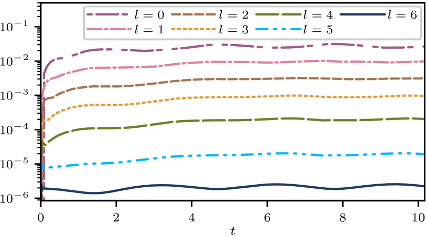
Figure 3: This figure shows the L2 norm of the error in the scalar field for a mesh that contains both DG and FV elements. We show the results for seven resolutions corresponding to h-refinement levels of $l=0,1,2,3,4,5,6$ and $7$. The error is consistent with 2nd order convergence.

In Fig. 3 we show how the numerical error converges to zero with resolution. Our method is consistent with second order convergence. While second order convergence may not sound too impressive, we note that in shocked regions we cannot expect more than first order convergence in any case. Thus, our method is adequate when used in elements with shocks. Our plan is then to use this FV method only in the elements where the matter is not smooth, while we plan to use the DG method everywhere else. In this way we should get the benefits of both FV and DG as suggested in [87, 65].

IV.2 Special relativistic blast wave tests

As a next step, we propagated a so-called special relativistic blast wave in one dimension. The initial setup has of discontinuities in the matter fields of $\rho_{0}$ and $P$, as in a Riemann problem. We study the case from [120] with $(\rho_{0},P,v_{x})$ given by

$$(\rho_{0},P,v_{x})=\left\{\begin{array}[]{ll}(10.00,13.33,0.00)&x\leq 0.5,\\ (1.00,0.00,0.00)&x>0.5.\end{array}\right.$$ (55)

We also use the analytic solution from the same article to check the accuracy of our simulation result. We then evolve the initial discontinuity from Eq. (55) using the full GRHD equations on a fixed Minkowski metric. For these tests, the time step was set according to the prescription in Sec. III.3.

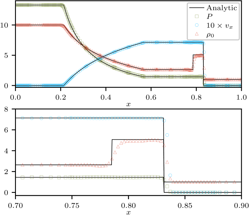
Figure 4: The plot shows blast wave profiles for pressure $P$, rest-mass density $\rho_{0}$ and speed $v_{x}$ (times 10) at $t=0.4$ after evolving the initial shocks in $P$ and $\rho_{0}$.

We set up the mesh with $16$ adjacent Cartesian elements along the $x$-axis. Initially, we set the element at the left boundary and the middle element containing the initial discontinuity to FV/FD containing $24$ equally spaced grid points, and the rest of the elements to DG, with $12$ grid points. During the evolution, we use our TEI from Sec. III.7 to decide if an element should use the DG or FV/FD method. For this case, we switch off the criterion from Eq. (50), as the purpose of it is to handle low density regions present in neutron star simulations, which is not relevant in this simulation. We also switch off the RDMP criterion, as it activates in regions where the analytic solution has zero slope, due to small amplitude variations in the numerical solution. These small amplitude variations can also trigger the Persson indicator if not relaxed enough. So, for the condition from Eq. (52), we choose $\alpha_{N}^{\mathrm{evo}}=4$ for the DG elements and $\alpha_{N}^{\mathrm{evo}}=5$ for the FV/FD elements. These values are lower than what we use for our star simulations in Secs. IV.3.2, IV.5.3 and IV.6, where we choose more conservative ones that result in more elements using FV/FD.

In Fig. (4) we plot the primitive variables. We show the entire mesh (top plot) as well as the contact discontinuity and the shock front (bottom plot), after evolving until time $t=0.4$. We see that the elements near the non-smooth regions evolve with FV/FD, while most other elements evolve with DG, as can be seen from the top plot. In both plots, we see that the fields in our simulation agree very closely with the analytic solutions that are plotted as solid black lines. This demonstrates that our hybrid DG+FV/FD method can successfully handle evolutions of shock fronts in matter fields, which is a crucial initial test, as such hydrodynamic shocks are known to develop during late inspiral and merger phases of a binary neutron star merger.

IV.3 Stable configuration (S)

This first case (S) starts with initial data for a static TOV configuration for testing stability and robustness of our program. Although we start with a static star, it gets perturbed through numerical errors throughout the duration of the simulations. Case (S) was simulated successfully with pure DG as well as DG+FV/FD. In (S), for setting up the initial data, we use a polytropic EoS which has the form in Eq. (24) while we evolve with the “gamma-law” EoS, which is of the form in Eq. (25) that allows for heating. We use this EoS for all the neutron star simulations of all the setups in Table 1. Similarly, for all the neutron star simulations in this paper, we use the Rusanov or local Lax-Friedrichs (LLF) flux for the evolution of the hydrodynamic (hydro) system, while we use the so-called “upwind” flux for the metric evolution with the GH system. Both of these numerical flux implementations are the same as described in Sec. 2.3 of [76].

IV.3.1 Pure DG (S) simulations:

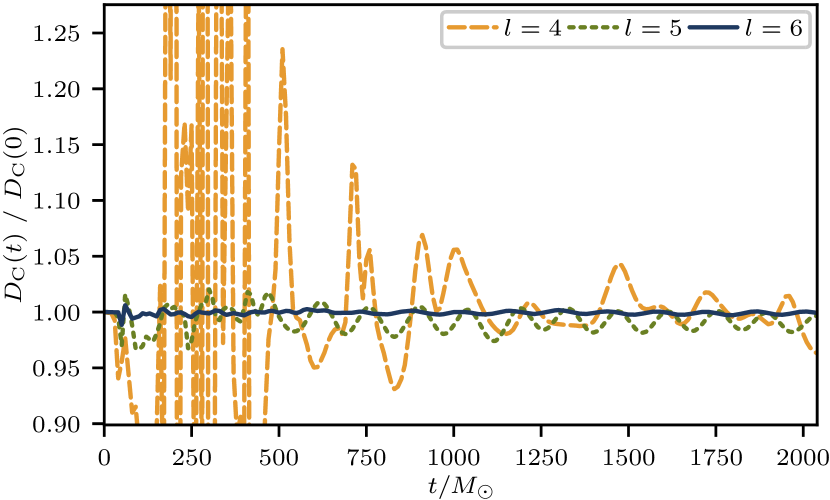
Figure 5: This figure shows central density $D_{\mathrm{C}}$ for (S) with pure DG simulations corresponding to h-refinement levels of $l=4,5$ and $6$, normalized to the initial value. Large amplitude Gibbs oscillations originating from the star surface spread across it generating large amounts of noise. This is especially true near the beginning, but continues to plague the lowest resolutions throughout. As resolution increases, the star settles down into more systematic oscillations consistent with the star’s fundamental oscillation frequency.

For the DG case, we set up the mesh using a cubical patch at the center, surrounded by $6$ cubed sphere patches on all sides, which in turn have another layer of $6$ cubed sphere patches forming a spherical shell covering them, resulting in total 13 patches. We then h-refined the central cubical patch successively $4$, $5$ and $6$ times, while refining all the other patches one time less in all the cases, resulting in $10240$, $81920$, and $655360$ total elements after h-refining. In each of these elements, we use $5\times 5\times 5$ grid points. The star is contained in the central cube with side length $32$, which is centered on the star, while the outermost boundary of the entire mesh is at 320. The resultant initial number of elements across the star for the $l=4,5$, and $6$ are stated in Table 2. We set the time steps for the different resolutions to be $0.1$, $0.05$ and $0.025$ respectively. For the artificial atmosphere, we set $f_{\mathrm{atmo,level}}=10^{-12}$, $f_{\mathrm{atmo,cut}}=1.01\times 10^{-12}$, $f_{\mathrm{atmo,max}}=10$, $\epsilon_{\mathrm{atmo,max}}=0.1$, and $(Wv)_{\mathrm{atmo,max}}=0.01$ as per the description in Sec. III.5.1. We also apply our positivity limiters with elementwise limiting of $D$, $\tau$ and $S_{i}$, but not the pointwise fixes described in Sec. III.5.2.

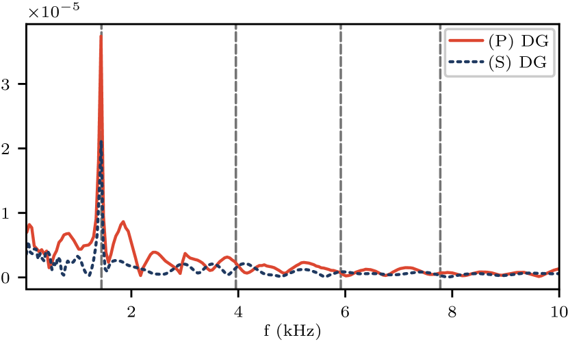
Figure 6: This figure shows the Fourier spectrum of the central point density $D_{\mathrm{C}}$ for (S) and (P) with pure DG for the simulation with $l=5$ levels of h-refinement for each case. The dashed vertical lines correspond to the expected frequencies for the various oscillations modes of the star, as stated in [121]. We see that the frequency for the principal mode from the oscillations matches perfectly with the theoretical value [121]. The higher modes are not obtained as pure DG simulations have too much noise due to Gibbs oscillations.

This limiter treatment is essentially the same as that described in [76]. We restrict the lower limit of $D$ to $10^{-12}\rho_{0,\mathrm{max}}(t=0)$ and $\tau$ to $0$, while enforcing $S<D+\tau$, as described when limiting. For the matter fields, as per Eq. (44), the filter uses $s=32$, while we use $s=40$ for the GH system. For both cases we have $\alpha_{f}=36$. For these simulations, we do not use the conserved to primitive variable conversion prescription mentioned in Sec. III.6. We retain the method for conversion described in Sec. 4.3.1 of [76]. This is because we performed simulation for the same physical system successfully under Cowling approximation with this method that has been presented in Sec. 4.3.4 in [76]. For the GH system we set the constraint damping parameters to be $\gamma_{0}=0.1$, $\gamma_{1}=-1$ and $\gamma_{2}=1$. The gauge is set such that the gauge source function is initialized according to the initial metric and then is kept constant throughout the simulation, i.e, we set

$$H_{\alpha}(t=0)=-\Gamma_{\alpha}(t=0),\quad\partial_{t}H_{\alpha}=0.$$ (56)

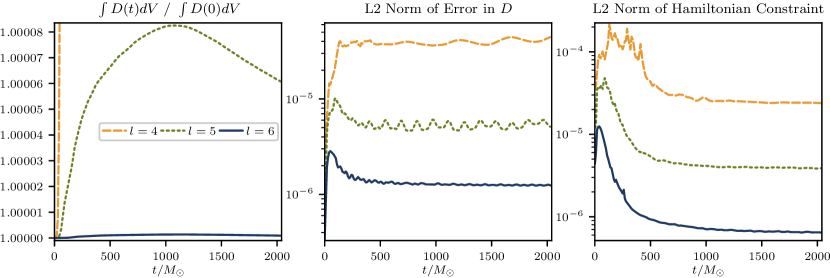
Figure 7: This plot shows three quantities for (S) with pure DG for resolutions $l=4,5,$ and $6$: total rest mass $\int DdV$ in entire mesh normalized to the initial value (left), L2 norm of error in $D$ (center), and L2 norm of the Hamiltonian constraint. We can see that mass conservation improves significantly with resolution, and the error quantities show convergent behavior. Here $dV=\sqrt{\gamma}d^{3}x$. The legend applies to all plots.

The run with $5$ times h-refined central cube was evolved stably until a time of $t=5000M_{\odot}$, even though the plots for this case only show data until $t=2000M_{\odot}$ time due to high computational costs. As can be seen from Fig. 5, the central density oscillates with time, with higher erratic oscillations towards the beginning. These errors are larger in the beginning in this pure DG simulation due to strong Gibbs oscillations arising from the surface of the star. This is because in the initial setup, the non-smooth feature on the surface of the star is at its sharpest, which produces large Gibbs oscillation in the DG scheme, as the surface lies in the middle of elements. These oscillations spread throughout the star and produce strong numerical disturbances. However, as the simulation progresses, our stabilizing mechanisms such as the positivity limiters, filters and the atmosphere damp the spurious Gibbs oscillations, which leads to smoother star oscillations. Hence, at later times, we see a systematic oscillation for the two higher resolutions, which is in agreement with the spectrum expected from such a setup, as can be seen from Fig. 6, that shows the Fourier spectrum of the central density $D_{C}(t)$ for the case with $5$ central refinement levels for (S) with pure DG. In this figure we see that the principal frequency matches the predicted value from literature [121]. The higher modes are buried in numerical noise due to the lack of resolution. Note that the numerical noise in the oscillations decreases with increasing resolution. We see the highest resolution is demonstrating consistent and persistent oscillations at the proper frequency, while for the middle resolution, they get damped slowly by the filters we apply. The lowest resolution of $4$ central refinement levels is swamped by Gibbs oscillations, and is depicted only to show improvement with resolution. We next consider mass conservation by looking at the volume integral of the rest mass density $D$ shown in the left plot of Fig. 7. It is very clear that mass conservation improves drastically with increasing resolution. The small amount of discrepancy in the highest resolution is attributed to the fact that we use positivity limiters that conserve the mass only when the element average is above the limits imposed. Furthermore, pointwise corrections to $D$ arise due to the atmosphere treatment. In this case, the $D$ value is pushed up whenever it wants to fall below the floor value set by us. Hence, in these situations the integral can increase.

We also study error quantities such as the L2 norm of the error in the conserved density $D_{\mathrm{C}}$ and the Hamiltonian constraint. We look at these quantities in the central box to get a true representation as that is where the star is located, while the rest is atmosphere. These are shown in the center and right plot of Fig. 7. As can be seen, these demonstrate convergent behavior with increasing resolution, with a measured convergence order of $2.6$ for both $D_{\mathrm{C}}$ and the Hamiltonian constraint.

We have also performed strong scaling tests with this (S) setup with pure DG, to demonstrate Nmesh’s capability to scale efficiently on a large number of computational cores or processors. This is shown in Fig. 8. This plot shows speed up vs. number of cores used for the run. Speed up when using $N$ number of compute cores is defined as $t_{r}(1)/t_{r}(N)$, where $t_{r}(N)$ is the run time measured for $N$ cores, with each core running one MPI process. Since a single MPI process cannot obtain enough memory for the simulations, $t_{r}(1)$ is estimated from $t_{r}(1)=N_{\mathrm{min}}t_{r}(N_{\mathrm{min}})$, where $N_{\mathrm{min}}$ is for the run with the lowest number of MPI processes performed in each case.

We performed these runs on both the Bridges-2 and Expanse supercomputers. In our case, we have $N_{\mathrm{min}}=3$ for the Expanse supercomputer and $512$ for the Bridges-2 supercomputer, which is used for the data in Fig. 8. We go up to $4096$ cores on Expanse and $6400$ cores on Bridges-2, which were the maximum core count available to us in the respective computers. The simulation we tested this with had total $262144$ elements in the mesh. We plot both the real simulation run time data and the ideal ones for the number of cores we have in each of the cases, and show the speedups for both. The ideal speed-ups are calculated from the $t_{r}(N_{\mathrm{min}})$, as is the usual custom in such scaling estimates. We can see that we obtain good strong scaling, as the real speedups not only rise almost in a straight line, but track the ideal lines very closely. The fact that they overshoot somewhat is because we have only an estimate from $t_{r}(1)$ from $t_{r}(N_{\mathrm{min}})$. This confirms that Nmesh scales efficiently with an increasing number of cores or MPI processes.

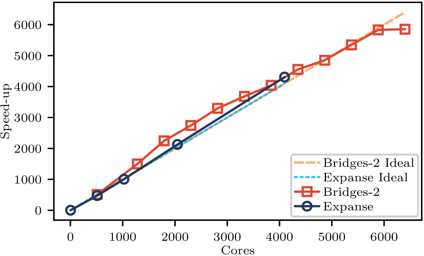
Figure 8: This plot shows speedup data for strong scaling test on Bridges-2 and Expanse for the pure DG (S) simulation with $262144$ elements. The dashed lines represent ideal speedup curves extended till the range of CPUs used for each supercomputer, while the solid lines represent the actual measured data for Nmesh. As we can see, the ideal and real data are in good agreement, demonstrating strong scaling.

IV.3.2 DG+FV/FD hybrid (S) simulation:

Figure 9: Initial mesh in the $xy$-plane from the (S) simulation with the hybrid DG+FV/FD evolution method. Top left: the star; top right: the central cube; bottom left: upto cubed sphere layer surrounding cube; bottom right: the entire mesh. The elements with denser, equally spaced grid points, are the ones using FV/FD. The DG elements are the ones with sparser, unequally spaced grid points. The color map shows the rest mass density $\rho_{0}$ profile. We see that only the troubled region at the star surface is initially set to use FV/FD.

We also evolve (S) with our hybrid DG+FV/FD scheme. In the elements that use FV/FD, we use the WENOZ₂ reconstruction scheme as described in Sec. III.2. Before using combined DG+FV/FD method, we have performed tests with pure FV/FD with the WENOZ₂ to validate our new method. However, we chose case (U) for these instead of (S), as it is significantly more challenging, and hence offers much more robust and general conclusions. These results are presented in Sec. IV.5.1 and IV.5.2. For the WENOZ₂ method in this case, we turn on extrapolation near the boundary as per the $w=4/3$ setup for Eq. III.2 described in Sec. III.2. Hence, we also switch on the cutoff levels for using $w=1$ as when $\rho_{0}<10^{-9}\rho_{0,max}(t=0)$ or $\epsilon<10^{-9}\epsilon_{max}(t=0)$, as described there. When the surface points of neighboring elements do not coincide, we use parabolic interpolation to exchange data between neighboring elements at the boundary. In the FD scheme used for the GH system we use fourth order dissipation in the interior of the elements (see Eq. (33)) with $\sigma=0.1$. Since we want the high order WENOZ used in the interior of elements to dominate the result, we increase the number of points in each direction in each FV/FD element to $n=16$, while in the DG elements, we use half as many points ($n=8$), as DG can provide high accuracy with lower number of points in the smooth regions. Each element then has $n\times n\times n$ total points. For this simulation, we set up the mesh similar to what we use for case (B), which is described later in Sec. IV.6, as they are the same star, with and without an imparted boost. The detail of the initial mesh can be seen from Fig. 9, which shows plots on the $xy$-plane. In the left top plot of the figure, we see the zoomed in view of the star. Initially, we set FV/FD only at the troubled region at the edge of the star. In order to determine which elements should be set to FV/FD at the initial time, we look at the coefficients of $\rho_{0}$ in an expansion in Legendre polynomials, as described in Sec. 2.5 of [76]. As we go from lower to higher order coefficients, we find a much slower drop off for elements that contain the star surface, than for elements in the star interior. We use this drop off to initially set only the elements containing the star surface to use FV/FD. These are recognizable from the denser grid lines as FV/FD uses twice as many points as DG. The initial number of DG and FV/FD elements across the star is given in Table 2. Next, in the top right plot we see the central cubical region, which is the best resolved region of the mesh. Here the size of this cube is $62$. However, as we can see, the resolution is not uniform. This is because we do not apply uniform h-refinement to the entire mesh. We h-refine a spherical region of radius $15$ centered on the star to $l=5$ times, which is the highest refined region in the mesh. The h-refinement is then dropped by one level as we move away from the star, with the different h-refinement spheres having radii $15,30,60$ and $120$. These successive regions can be seen in the plots on the top right, bottom left and bottom right. In the left bottom picture, we see the mesh up to the first cubed sphere patches surrounding the central cube, up to a distance of $104$. The last bottom right picture shows the entire mesh, which has a radius of $208$. In total, we have 13 patches similar to the setup in Sec. IV.3.1. The time step is set as per Sec. III.3.

For the atmosphere we use the values $f_{\mathrm{atmo,level}}=10^{-11}$, $f_{\mathrm{atmo,cut}}=10^{-9}$, and $f_{\mathrm{atmo,max}}=1$, as this is the setup we also use for (U) and (B) simulations with DG+FV/FD, which are described later. The other atmosphere limits are still maintained at $\epsilon_{\mathrm{atmo,max}}=0.1$, and $(Wv)_{\mathrm{atmo,max}}=0.01$. Here, we employ the entire limiting process described in Sec. III.5.2 for $D$, $\tau$ and $S_{i}$, including both elementwise and pointwise limiting. For this purpose, we set $f_{S}^{\mathrm{lim}}=0.99$. In this simulation, we use the conversion procedure from conserved to primitive variables stated in Sec. III.6, setting $\epsilon_{\mathrm{floor}}=0.0$. The constraint damping parameters for the GH system are set to be the position dependent functions of the form from Eq. (5) along with Eqs. (59)-(61). The gauge is chosen to be the harmonic gauge, where the gauge source function is set as $H_{\alpha}=0$. In the DG elements, we filter the conserved matter variables $D,\tau$ and $S_{i}$ with $s=40$, while using $s=64$ for the GH variables of the evolved metric and its derivatives. We maintain $\alpha_{f}=36$ for both. No filters are used in the FV/FD elements, as dissipation plays the counterpart role. When incorporating the TEI described in Sec. III.7, we set the value of $\displaystyle\alpha_{N}^{\mathrm{evo}}$ from Eq. (52) in the elements using DG to be $8$ and to $9$ in the elements using FV/FD. For this criterion, we only consider the coefficients that are greater than $f_{\mathrm{unfiltered}}=0.9$ times their unfiltered value. We set the cutoff from Eq. (50) as $\rho_{\mathrm{cut,low}}=10^{-4}\rho_{0,\mathrm{max}}(t=0)$ and $\displaystyle\rho_{\mathrm{cut,hi}}=\displaystyle 10~\rho_{\mathrm{cut,low}}$.

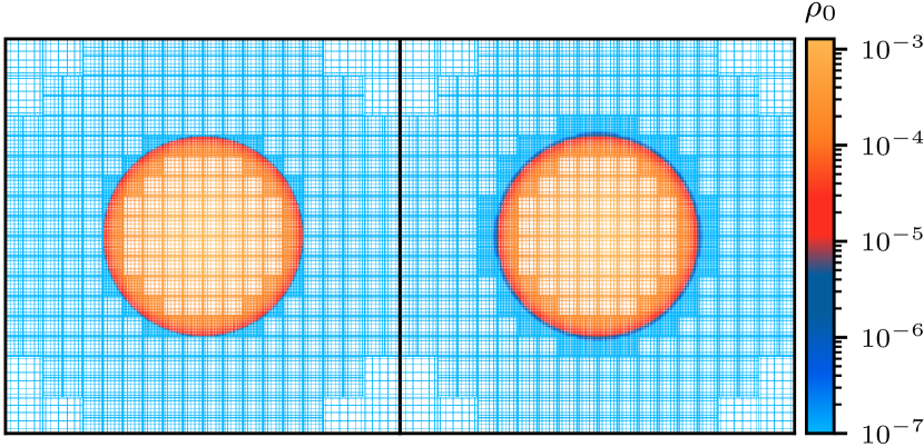
Figure 10: A $xy$-plane slice of the star from the (S) simulation with the hybrid DG+FV/FD method at two times. Left: $t=0M_{\odot}$; right: $t=1000M_{\odot}$. We see that only the star surface continues to evolve with FV/FD at $t=1000M_{\odot}$, showing proper TEI functioning. The TEI adapts to the slight expansion of the star surface.

We show the density $\rho_{0}$ plotted as a colormap on the mesh wireframe in the $xy$-plane in Fig. 10, zooming in on the star. The initial setup can be seen in the left plot. The right box of Fig. 10, shows $\rho_{0}$ after evolving to time $t=1000M_{\odot}$. We see that the star has expanded slightly from the initial configuration. The number of elements using FV/FD also increases accordingly to adapt to the star surface as it expands. Still, only the surface of the star is evolved with FV/FD, indicating proper functioning of our TEI.

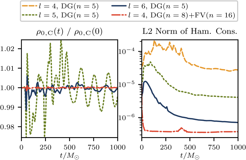
Figure 11: This figure compares results from DG+FV/FD (S) simulation with pure DG (S) simulations for central density $\rho_{0,\mathrm{C}}$(left) and L2 norm of Hamiltonian constraint in the central cube (right). We see that the noise in $\rho_{0,\mathrm{C}}$ for the DG+FV/FD simulation is significantly lower than all the pure DG simulations. For the Hamiltonian constraint, the DG+FV/FD simulation settles down to its steady value faster than all DG simulations, and remains lower as well.

Lastly, we look at the central density $\rho_{0,\mathrm{C}}(t)$ normalized to the initial value (left plot) and the Hamiltonian constraint’s L2 norm in the central box (right plot) in Fig. 11, which are the representative quantities we study for all the DG+FV/FD simulations, including for (U) and (B) described later. For the Hamiltonian constraint, we compare all the (S) simulations. For $\rho_{0,\mathrm{C}}(t)$, we exclude the lowest resolution pure DG run as we know it has large noise in $\rho_{0,\mathrm{C}}(t)$. It should be kept in mind when making these comparisons, that the bulk of the mesh for our DG+FV/FD scheme has a resolution that falls in between the $l=4$ and $l=5$ cases for the pure DG simulations in Sec. IV.3.1. Even though the central h-refinement sphere for DG+FV/FD uses $l=5$, the dimension of the central cube is much larger than the previous setup. However, as the DG scheme is expected to demonstrate exponential convergence when increasing the order of the basis polynomials, the choice of $n=8$ for the DG elements in this DG+FV/FD evolution should give us much more accurate results for the same h-refinement level. As was mentioned in Sec. IV.3.1, the $l=4$ level was kept in the discussion only as a reference for improvement of results with increasing resolution. We started getting reliable results only from the $l=5$ resolution onwards. Keeping all these in mind, we expect the DG+FV/FD case to be the hybrid counterpart closest to the pure DG scheme of $l=5$ resolution. As can be seen from the left plot for $\rho_{0,\mathrm{C}}(t)$ in Fig. 11, the central density for DG+FV/FD essential settles down immediately into systematic oscillations compared to the pure DG runs. Additionally, the oscillation amplitude is much smaller. This is because the FV/FD at the surface of the star eliminates the Gibbs oscillations that plague the pure DG simulations at early times, when the perturbations from the numerical errors kick in. This is also reflected in the Hamiltonian constraint shown on the right of Fig. 11, which settles down much faster for the DG+FV/FD case. In fact, the results settle to a steady state even faster than the $l=6$ pure DG run, and to an even lower value. The comparable case of $l=5$ still remains at a level much above the DG+FV/FD case. Hence, we can see that the DG+FV/FD simulation performs significantly better than the equivalent pure DG simulation.

IV.4 Perturbed configuration (P)

Having confirmed the robustness of our program through (S), we next apply a pressure perturbation to the star at $t=0$. We call this case (P). The pressure perturbation is of the form $P+\delta P$ [122], with

$$\delta P=\displaystyle\lambda\cdot(P+\rho_{0}+\rho_{0}\epsilon)\sin\left(\displaystyle\frac{\pi r}{r_{\mathrm{surf}}}\right)Y^{0}_{2}(\theta,\varphi),$$ (57)

where $(r,\theta,\varphi)$ are the standard spherical coordinates, $Y^{0}_{2}(\theta,\varphi)$ is the $l=2$, $m=0$ spherical harmonic, and $r_{\mathrm{surf}}=8.1251439$ is the radius of the unperturbed star. Both $r$ and $r_{\mathrm{surf}}$ are in isotropic coordinates, which is the coordinate system used in the cubical patch in the center of our mesh in which we evolve the star. Once $P$ is set, we recompute the corresponding values for $\rho_{0}$ and $\epsilon$ for the initial setup using the EoS in Eq. (24). The metric variables are left unchanged and maintain their unperturbed TOV values as in (S). The magnitude of the perturbation parameter is set to $\lambda=0.05$, which is a reasonably strong perturbation.

Figure 12: This figure shows central density $D_{\mathrm{C}}$ for (P) with pure DG simulations corresponding to h-refinement levels of $l=4,5$ and $6$, normalized to the initial value. Same as for (S), substantial Gibbs oscillations spread across the star from the surface, generating large amounts of noise, especially for the low resolution. Once again, as resolution increases, systematic oscillations consistent with principal frequency of the star becomes more pronounced.

The remaining setup, apart from the pressure perturbation, remains exactly the same as the pure DG (S) simulation in Sec. IV.3.1. To study the effect of different resolutions, we again look at the central conserved density $D_{C}$ plot for the different refinement levels of $l=4,5$ and $6$, shown in Fig. 12. In this case, as there is an actual relatively stronger perturbation present, the oscillations in the central density are much more pronounced than in (S) where the oscillations were simply the result of much weaker perturbations form numerical noise. Again, we see that the $l=6$ case displays the expected behavior the best, while the lowest resolution of $l=4$ is once again swamped by Gibbs oscillations and numerical noise to the extent that we are unable to observe the characteristic oscillation we expect in this case. We again look at the Fourier transform of the central density in Fig.(6). Although the perturbation is significant, the deviation in the physical attributes such as mass and central density are within a margin such that characteristic spectrum is still in agreement with the (S) configuration as described in [121]. Hence, we still see the principal mode to be in perfect agreement with that predicted by theory. In fact, it is more pronounced as the oscillation is larger than (S). Once again, the higher modes are swamped by numerical errors.

The takeaway is that Nmesh is able to successfully evolve a perturbed star with gravity coupled to the matter fields with pure DG. The results agree with literature results, as can be seen from the principal oscillation frequency from the Fourier spectrum.

IV.5 Unstable configuration (U)

Having tested that our program successfully and stably handles the dynamics of the perturbed star in case (P), we move on to the case of a star with an initial configuration of a TOV star on the unstable branch (U), where ${\partial}m_{\mathrm{ADM}}/{\partial}\rho_{0,\mathrm{C}}<0$ [123, 124]. Here $m_{\mathrm{ADM}}$ is the so-called “ADM” mass of the star being defined from the Arnowitt-Deser-Misner formalism [111]. The initial data for this star is in a highly dense unstable equilibrium state [121]. As such, any initial configuration on the unstable branch migrates either towards a TOV configuration on the stable branch or collapses into a black hole depending on the nature of initial perturbations [125, 126, 121, 123, 127, 83, 124]. In this article, we want to study the case where the initial unstable TOV configuration migrates towards a stable TOV configuration. It is thus important to have an initial perturbation that drives the system in this direction.

This case is significantly more challenging than the previous ones, as the matter fields are much more dynamic and there are shocks, which are most visible in the $\epsilon$ field [121, 47]. Even though the matter fields such as $\rho_{0}$ and $\epsilon$ were not smooth at the star surface in (S) and (P), the non-smooth feature remained relatively localized to its initial position as the configuration did not change drastically. The only motion came from the comparatively much gentler oscillations arising from either numerical or the pressure perturbation. However, the star (U) expands and contracts violently as it gets displaced from the initial configuration. It shoots past its stable configuration and goes back and forth between relatively higher and lower central density configurations. For handling these violent motions and shocks in the matter fields, the DG method alone was not suitable. Even though the system did evolve without crashing with DG alone, the dissipation caused by the filters and limiters was so significant, that the results, at affordable resolutions, were not close to the well known expected behavior as stated in [121, 122]. Hence, to handle this case we had to fall back to the FV/FD method, which provides robust HRSC capabilities.

As our FV/FD method is a modified one, we started out by first evolving the case with pure FV/FD with WENOZ₂. We ran simulations with different resolutions for (U) to test behavior of results on the ANVIL supercomputer. We tested the results separately for p-refinmenet and h-refinement variations. We still used the mesh setup of a central cube surrounded by cubed sphere patches, with total $13$ patches as for (U) and (P). However, as (U) is initially much denser, it has a much smaller radius, and to better adapt to this smaller size, we set the length of the central cube to $16$. We use the position dependent constraint damping from Eq. (5) and Eqs. (59)-(61) and harmonic gauge with $H_{\alpha}=0$ for the GH system. The atmosphere is set such that $f_{\mathrm{atmo,level}}=10^{-11}$ and $f_{\mathrm{atmo,cut}}=10^{-9}$, $f_{\mathrm{atmo,max}}=1$, $\epsilon_{\mathrm{atmo,max}}=0.1$, and $(Wv)_{\mathrm{atmo,max}}=0.01$ as introduced in Sec. III.5.1.

IV.5.1 Varying p-refinement for pure FV/FD (U) simulations:

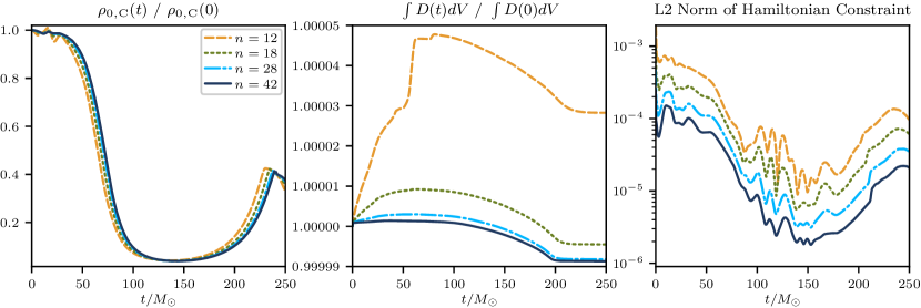
Figure 13: Results for p-refinements of $n=12,18,28$, and $42$ and h-refinememnt level of $l=3$ for the pure FV/FD simulation of (U) till the first peak when the star contracts. Left: central rest mass density $\rho_{0,\mathrm{C}}$(normalized to the initial value); center: rest mass $\int DdV$ in the central cube (normalized to the initial value); right: L2 norm of Hamiltonian constraint in the central cube. We see that the peak value of $\rho_{0,\mathrm{C}}$ is in good agreement with that in other simulations such as in [121]. The offset in time of the different resolutions is because the star gets displaced from the initial state at different times due to difference in perturbations from the different resolutions. The rest mass and the Hamiltonian constraint show convergent behavior.

For the case of p-refinement, we vary the number of points in each element in each direction to be $n=12,18,28$, or $42$, with $5$ elements across the star. Since we increase the number of points from the pure DG (S) and (P) setups and also made the central cube smaller, we lower the h-refinement level for these runs to $l=3$, so that the elements are larger, resulting in $6656$ total elements. The parameters for the limiters (see Sec. III.5.2) are the same as in Sec. IV.3.2. When converting from conserved to primitive variables, the procedure in Sec. III.6 is relaxed, and for this case we allow negative $\epsilon$ values by setting $\epsilon_{\mathrm{floor}}=-0.1$. Because of this, $\epsilon$ dips below $0$ for short periods of time in places where a shock forms when matter falls back on to the star during contraction due to numerical errors in the lower resolutions $n=12$ and $n=18$. Yet, for the higher resolutions of $n=28$ and $n=42$, $\epsilon$ remains positive. We do not apply filters to any of the variables here, as we are evolving with pure FV/FD and our WENOZ₂ scheme is capable of handling any non-smooth features. However, here we set $w=1$ in Eq. (III.2), thus dropping extrapolation near the boundary. At the boundary, when interpolation is needed for data exchange between neighbors, we use linear interpolation. One point away from element boundaries, we also add a second order dissipation operator to the GH system, by using the standard centered second derivative stencil there. The dissipation factor is set to $\sigma=0.1$. These extra modifications were done out of an abundance of caution. However, later studies have shown that they are not needed to keep the system stable. Consequently, they were not used in the more sophisticated hybrid simulations discussed below.

For the simulations with varying p-refinement discussed in this section and those with varying h-refinement discussed in the following Sec. IV.5.2, there was a discrepancy in our implementation of the derivatives ${\partial}_{i}\alpha$ needed in the source terms for the hydrodynamic variables outlines in Eq. (17). This was later discovered and fixed for all the other simulations. This discrepancy produced a maximum of $1.5\sim 2\%$ difference in the source terms, depending on the term considered. Incidentally, this maximum occurs very early in the simulation, just when the star gets displaced from its initial unstable equilibrium configuration. The magnitude of this difference then decreases significantly during the rest of the simulations. As such, this discrepancy essentially functions like a perturbation, which coincidentally has a form that drives the star towards the stable configuration. The magnitude of this perturbation is then also comparable to the perturbations usually applied in such studies [83, 126] and also to the density perturbation we use in Sec. IV.5.3.

Although the lower resolutions were continued until about a time of $t=900M_{\odot}$, we look at the results until time $t=250M_{\odot}$, where we have stopped our higher resolution runs because of computational cost. As can be seen from the left plot in Fig. (13), which shows the variation of central rest mass density $\rho_{0,\mathrm{C}}$, we have the simulation continuing through the first expansion phase of the star, starting from the initial highly dense unstable state, until it partially contracts back again for the first time. The oscillations seen in the beginning result from perturbations due to numerical errors, while the star is still hovering around the unstable equilibrium before migrating towards the stable one. As the star gets displaced from its initial state partially by perturbations arising from numerical errors, the time at which the star starts to expand from the initial compact state differs for the different resolutions. As such, the first major expansion phase is offset by different amounts in time for different resolutions.

For the reasons discussed below, we shift the star away from the center of the mesh for these (U) simulations. Due to h-refinement, the corners of eight elements meet at the mesh center. If the star is centered on the mesh, sharp features in the density form at the center in our simulations. Similar sharp features have been observed for this unstable star system in [123, 83]. However, simulations with conventional FV schemes as in [121] do not show such sharp features. As explained in [83], we believe that these features cannot be easily resolved by conventional FV methods, and are therefore not shown in much of the literature. Hence, to obtain results as close as possible to the standard 2D or 3D simulations for this setup [121, 128, 47], and for ease of comparison and vetting of results, we have decided to move the mesh so that the star center (located at the $(0,0,0)$) is at the center of an element. This suppresses sharp features in our simulations, as our FV/FD scheme acts like any standard FV method at element centers. For the simulations discussed below, the mesh is centered on the point $(1,1,1)$. Even with this setup there still remain some oscillations in the central density $\rho_{0,\mathrm{C}}$. However, the overall nature of our results agrees with standard results obtained with FV methods in 3 dimensions. Additionally, the variation of $\rho_{0,\mathrm{C}}$ with resolution in left plot of Fig. (13) is consistent with second order convergence.

From the center plot in Fig. 13 we see that mass conservation improves with resolution. For the highest resolution case, the mass remains almost constant until about a time of $t=100M_{\odot}$. Until this point, the bulk of the matter is contained in the innermost cube, which is the best resolved region. However, since the star is expanding, the matter gradually spills over into the surrounding cubed sphere patches. Since linear interpolation takes place at the element boundary between an element in the central cubical patch and an adjacent element in the cubed sphere region, the mass does not remain exactly conserved, causing the drop we see around this time. Furthermore, the resolution also drops in the elements in the cubed sphere region, which also contributes to the mass loss we observe. Lastly, the limiters and atmosphere treatment we apply perform pointwise fixes, that also contribute to this violation. At around $t=160M_{\odot}$ the central higher density region, containing matter with density above $10^{-2}\rho_{0,\mathrm{C}}(t=0)$, stops expanding, and starts contracting again. However, a lower density shell of about $10^{-2}\rho_{0,\mathrm{C}}(t=0)$ to $10^{-5}\rho_{0,\mathrm{C}}(t=0)$ continues to expand, going further into the less resolved region, which causes the $\int DdV$ quantity to keep dropping. This shell stops expanding at around $t=192M_{\odot}$, which is when we see the second stabilization of the mass. The overall takeaway again is that the mass conservation improves drastically with increasing resolution. The error caused by the interpolation, and the other factors converge away with increasing resolution, providing reliable results as we go to reasonably good resolutions.

Lastly, we look at the L2 norm of the Hamiltonian constraint violation of the central cube as although some matter eventually flows out of it, the majority of the matter still remains contained within it. Again we see convergent behavior with increasing resolution. For the constraint violations shown in Fig. 13, we find a convergence order of $1.5$.

Overall, we see that our results for the simulations agree with the expected behavior of the system as per standard literature. Additionally, results improve with resolution in systematic fashion for all the quantities we study.

IV.5.2 Varying h-refinement for pure FV/FD (U) simulations:

The setup of the patches in the mesh remains the same here as in Sec. IV.5.1. However, we use $n=16$ points in each direction in each of our elements. Furthermore, we no longer apply uniform h-refinement, and instead switch to the concentric spherical decreasing h-refinement regions centered on the star (see Fig. 9), introduced in Sec. IV.3.2.

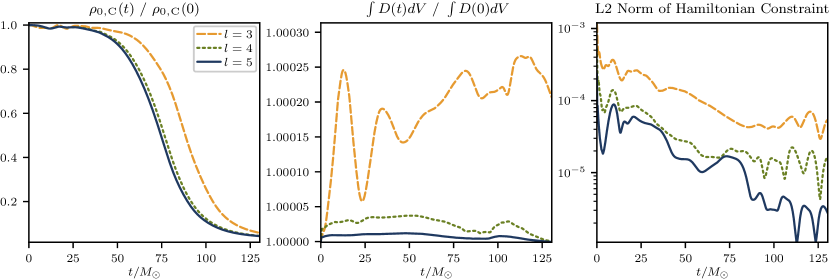
Figure 14: Results for central h-refinements of $l=3,4$ and $5$ with $n=16$ for the pure FV/FD simulation of (U). Left: rest mass density $\rho_{0,\mathrm{C}}$ (normalized to the initial value); center: rest mass in central cube (normalized to the initial value); right: L2 norm of Hamiltonian constraint in central cube.

The radius of the most highly refined region is chosen to be $30.5$ to ensure that the bulk of the matter is contained inside this region. The refinement is dropped by one level after radii $30.5,61,122$ from the origin, with the radius of the entire mesh being $200$. The resultant initial number of elements across the star for this setup are stated in Table 2. The central region refinements are chosen to be $l=5,4,3$ for the different cases. The center of the mesh is shifted to $(1,1,1)$, $(0.5,0.5,0.5)$ and $(0.25,0.25,0.25)$ for the three different resolutions respectively, to always have the star center at the middle of an element, similar to Sec. IV.5.1. The FV/FD related setup for this run is the same as the treatment of the FV/FD elements in the DG+FV/FD run for (S) in Sec. IV.3.2. This means, we switch on the extrapolation near the element boundary for WENOZ₂, use parabolic interpolation at the boundary, and limit dissipation to the interior of an element as in Eq. (34). The hydro setup also remains the same as in Sec. IV.3.2, and so does the GH system.

The behavior of the different quantities such as $\rho_{0,\mathrm{C}}$, $\int DdV$, and L2 norm of the Hamiltonian constraint in the central cube remain similar to that for varying p-refinement, as can be seen from the left, center and right plots in Fig. 14 respectively. We see systematic improvements in all the quantities with increasing resolution. Unfortunately, due to high computational cost, we could continue the highest resolution simulation to barely beyond the first expansion phase. This limits our capability to make strong conclusions, but we can still see that the results improve with resolution and are trending in a desirable fashion. The lowest resolution simulation was continued for much longer, the results for which can be seen in Fig. 15 by looking at the dashed line curves.

Figure 15: This figure shows $\rho_{0,\mathrm{C}}$ normalized to the initial value (left) and L2 norm of Hamiltonian constraint in central box (right) for the comparable pure FV/FD and DG+FV/FD cases for (U). Both have central h-refinement of $l=3$ and use $n=16$ in their FV/FD elements. Both simulations are in good agreement for both quantities. Furthermore, $\rho_{0,\mathrm{C}}$ agrees well with standard literature values [121].

We see the characteristic alternate peaks and troughs in the central density $\rho_{0,\mathrm{C}}$ with attenuating amplitude in the left plot, that is known to be the appropriate behavior of (U) setup when evolving with an EoS that allows for heating. In the right plot we see that the L2 norm of the Hamiltonian constraint also goes through the undulations as the matter flows in and out of the central box, while maintaining overall stability. Given that the lowest resolution shows stable and accurate behavior in the long term simulation, and the shorter runs show convergent behavior with increasing resolution for the various quantities, we can cautiously conclude that this setup for the simulations are handled well with Nmesh, and we expect that we will be able to see proper convergent behavior with longer runs and more different resolutions in our future work. Having said that, for these short duration runs, we find that $\rho_{0,\mathrm{C}}$ in Fig. 14 is consistent with convergence of order $2.55$ with resolution, while the Hamiltonian constraint L2 norm in Fig. 14 tends towards 2nd order convergence.

IV.5.3 DG+FV/FD (U) simulation:

Having confirmed the robustness and soundness of our new FV/FD method, we next evolved (U) with the hybrid DG+FV/FD method. For this case, the setup related to the mesh, WENOZ₂, FV, FD, metric and hydro evolutions remain same as cases with h-refinement $l=3$ and $4$ and number of points $n=16$ in the previous section IV.5.2. However, we now incorporate our TEI exactly the same way we did for the DG+FV/FD simulation of (S) in Sec. IV.3.2. The associated treatments of all the aspects of the DG elements also remain the same as in Sec. IV.3.2. For these simulations, we apply a perturbation to $\rho_{0}$ of the form

$$\delta\rho_{0}=\displaystyle\frac{\lambda\rho_{0}}{\sqrt{4\pi}}\cos\left(\frac{\pi r}{2r_{\mathrm{surf}}}\right)$$ (58)

at the initial time. Here $r=\sqrt{x^{2}+y^{2}+z^{2}}$ is the distance from the star center in isotropic coordinates, and $r_{\mathrm{surf}}=4.2677044$ is the radius of the unperturbed star (also in isotropic coordinates). We choose $\lambda=-0.01$ so that the magnitude of the perturbation remains within $1\%$ as is the usual order of magnitude chosen for such perturbations [83, 126]. Additionally, the sign is chosen to drive the star towards the stable TOV configuration instead of a black hole. The reason for choosing this perturbation is that if left solely to perturbations arising from numerical errors, the star would sometimes collapse to a black hole, depending on the resolution, mesh setup and other such factors. Since here we wish to study the migration of an unstable star to a stable TOV star, we use this perturbation to ensure that the unstable star is consistently pushed in this direction, and not in the direction of forming a black hole [125, 126, 121, 123, 127, 83, 124].

We again check that our TEI is working properly by verifying that only the elements only near non-smooth regions switch to FV/FD. Figure 16 shows the density on the mesh wireframe, similar to Sec. IV.3.2, to check which parts have switched to FV/FD, while zooming in onto the central cube in the $xy$-plane. Unlike for (S), we cannot focus only on the central cube this time, as the matter flows out into the rest of the mesh over time. We pick four time frames to look at in this figure. The top left figure shows initial $t=0M_{\odot}$ setup, where we set every element to FV/FD. This is because the star surface has a much steeper rise in the matter fields, and so we simply set all elements to FV/FD initially to be cautious, letting the TEI set the appropriate elements to DG after eleven time steps.

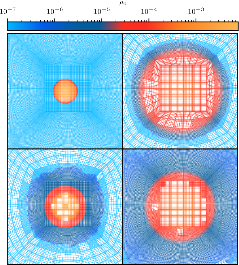
Figure 16: Part of the mesh in the $xy$-plane from (U) simulation with hybrid DG+FV/FD evolution method at four different times. Top left: $t=0M_{\odot}$ (initial state); top right: $t=136M_{\odot}$ (first minimum of $\rho_{0,\mathrm{C}}$); bottom left: $t=232M_{\odot}$ (next peak with $\rho_{0,\mathrm{C}}\sim 0.4\rho_{0,\mathrm{C}}(t=0)$); and bottom right $t=320M_{\odot}$ (second minimum of $\rho_{0,\mathrm{C}}$). FV/FD elements have denser equally spaced points, while DG has sparser unequally spaced points. We see that our hybrid scheme’s TEI successfully tracks the low density (shown through the colormap) troubled region as the star expands and contracts.

The next plot (top right) at $t=136M_{\odot}$ is close to when the central density of the star reaches the first minimum after the star expands, in the context of left plot of Fig. 15. Only a narrow troubled region at the boundary of the star uses FV/FD, which has matter density between $10^{-2}\rho_{0,\mathrm{C}}(t=0)$ and $10^{-4}\rho_{0,\mathrm{C}}(t=0)$. The rest of the mesh elements are evolved with DG. Next (bottom left) time shown is $t=232M_{\odot}$, which is close to the time when the star first fully recontracts, producing the central maximum of $\rho_{0,\mathrm{C}}(t)\sim 0.4\rho_{0,\mathrm{C}}(t=0)$ in left plot of Fig. 15. The shell of FV/FD elements also follows the star surface. However, now the star is starting to get larger, with the density range $10^{-2}\rho_{0,\mathrm{C}}(t=0)$ to $10^{-4}\rho_{0,\mathrm{C}}(t=0)$ spreading further from the bulk of the matter in the center. It should be kept in mind that even though we are looking only at the $\rho_{0}$ field here, there are sharp features, and even shocks that are particularly visible in the $\epsilon$ field, linked to these fast moving low density shells, which has also been observed in [121, 47]. The TEI picks up on them and switch from DG to FV/FD as necessary. Hence, a thicker band of elements around the star switches to FV/FD. The center has also adopted FV/FD as there are oscillations at the center due to matter falling into it from all sides when the star contracts. Similar oscillations have been also observed in [83], when dissipation is low enough compared to more traditional schemes. Lastly, we show time $t=320M_{\odot}$ in the bottom right plot, corresponding to the second minimum in the left plot of Fig. 15 when the star has once again expanded. Here we see that the troubled region has spread considerably and most of the field of view in the plot is covered by FV/FD elements, while DG is used in the smooth interior of the star. Of course, if we zoom out, most of the rest of the mesh is still largely evolved with DG. From these plots, we can determine that our TEI functions properly, and can track the troubled region appropriately even in a case like (U) where the star is undergoing much more violent motions through expansion and contraction than the considerably benign case (S) of Sec. IV.3.2.

We also check the behavior of $\rho_{0,\mathrm{C}}(t)$ and L2 norm of Hamiltonian constraint in the central cube for the DG+FV/FD runs with two different h-refinement levels, and compare them to the same quantities from our FV/FD runs with corresponding resolutions, as shown in Fig. 15 and Fig. 18. The lowest resolution runs provide comparison for longer time, as they are computationally cheapest. We see that the results for $\rho_{0,\mathrm{C}}(t)$ with DG+FV/FD runs match reasonably well with their same resolution pure FV/FD counterparts, considering the time offsets owing to difference in nature of the initial perturbations. The Hamiltonian contraint is lower for the same resolution for the DG+FV/FD simulation than the pure FV/FD simulation. Additionally, the Hamiltonian constraint improve from $l=3$ to $l=4$ resolution when considering only the DG+FV/FD curves, while $\rho_{0,\mathrm{C}}(t)$ shows similar behavior. These give us confirmation that the DG+FV/FD evolutions are performing well.

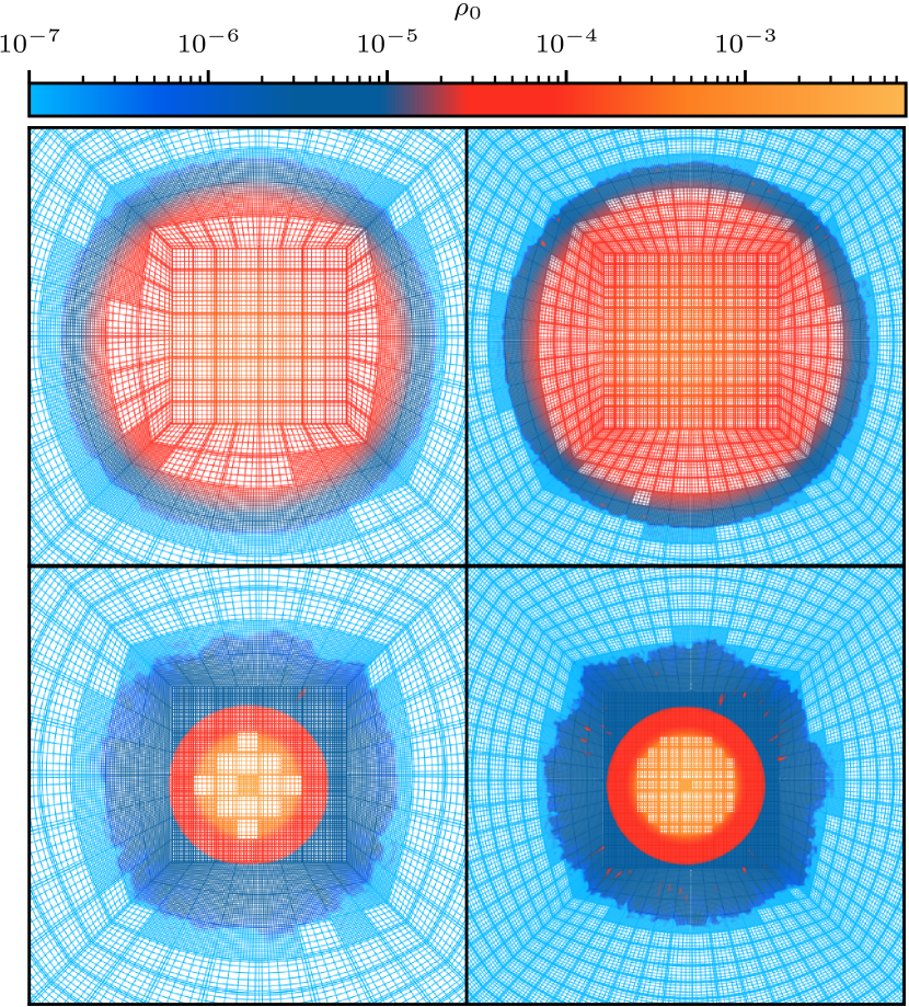
Figure 17: Portion of the mesh in the $xy$-plane from the (U) simulation with the hybrid DG+FV/FD method with different central h-refinmenet levels. Top Left: $t=132M_{\odot}$ for $l=3$ and top right: $t=148M_{\odot}$ for $l=4$; bottom Left: $t=232M_{\odot}$ for $l=3$ and bottom right: $t=228M_{\odot}$ for $l=4$. Both show $\rho_{0}$ close to the time when $\rho_{0,\mathrm{C}}$ reaches its first minimum and the following maximum. We see that the width of the region evolved with FV/FD decreases with increasing h-refinement, as the troubled region is concentrated in the non-smooth region near the star surface.

Last, we compare the TEI perfromance for the DG+FV/FD simulations with different levels of h-refinement in Fig. 17. This provides another crucial test, as with increasing h-refinement the TEI should hone in on the troubled regions near the star surface, thus using FV/FD in a smaller region. We see this successfully carried out in Fig. 17, where the lower h-refined simulation in the left plots show a thicker region of FV/FD elements, as compared to the counterparts from the higher h-refined simulation on the right. The top plots correspond to the time when the star has expanded fully for the first time, and $\rho_{0,\mathrm{C}}$ has reached its first minimum, while the bottom plots are for the following maximum in $\rho_{0,\mathrm{C}}$, when matter has fallen in. For both these states of the star, the times for the two resolutions of $l=3$ and $l=4$ has been chosen while accounting for the time offset in the dynamics of the two resolutions to achieve a faithful comparison. So, we can conclude from these plots that the TEI perfroms properly and retains DG in more elements as the element size decreases with increasing h-refinement.

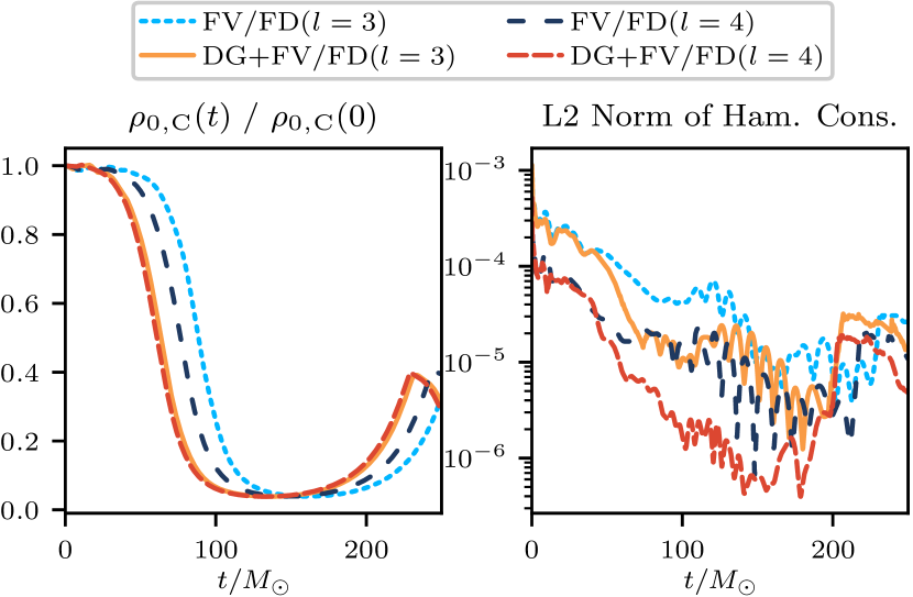
Figure 18: This plot shows central density $\rho_{0,\mathrm{C}}$ normalized to the initial value (left) and L2 norm of Hamiltonian constraint in the central cube (right) for comparable cases with pure FV/FD and DG+FV/FD for (U) with central h-refinement levels of $l=3$ and $l=4$. We see that for $\rho_{0,\mathrm{C}}$ the corresponding runs with pure FV/FD and DG+FV/FD are in good agreement. For the constraint violation, DG+FV/FD performs somewhat better than the pure FV/FD runs in the central cube, both in terms of the overall violation level, and the convergence behavior.

Hence, from all these results, we can conclude that our TEI can successfully handle not only the simple case of (S), but also the far more challenging case of (U). Additionally, the results obtained from the combined DG+FV/FD simulations agree well with the expected results for this scenario, and also improve with increasing resolution.

IV.6 Boosted configuration (B)

Figure 19: Portion of the mesh in the $xy$-plane from the (B) simulation with $v_{\mathrm{CoM}}=0.5$ using the DG+FV/FD evolution method at four different times. Top left: $t=0M_{\odot}$; top right: $t=40M_{\odot}$; bottom left: $t=88M_{\odot}$; and bottom right $t=132M_{\odot}$. The elements with denser, equally spaced grid points, are the ones using FV/FD. The DG elements are the ones with sparser, unequally spaced grid points. The colormap shows the rest mass density $\rho_{0}$. We see that the TEI nicely track the surface of the star and use FV/FD only in that region. Furthermore, we also see the adaptive mesh refinement spheres track the star. The simulation continues smoothly even beyond the central cubical region.

The last case we study is the boosted star (B), that has an initial boost applied to (S). We evolve two (B) setups with boost applied such that the center of mass(CoM) of the star has a velocity of $v_{\mathrm{CoM}}=0.1$ and $0.5$ diagonally along the $xy$-plane. (B) again proves too difficult to evolve with pure DG, as large unphysical Gibbs oscillations develop that reduce the accuracy significantly. Hence, we again turn to the DG+FV/FD method. Almost every aspect of the simulations setups for (B) remian the same as the (S) simulation in Sec. IV.3.2, with a few modifications, as we impart a boost to that very star in the simulations of this section. The larger dimension of $62$ of the cube, compared to the (U) setup and pure DG (S) setup, is chosen for allowing the star to travel for longer in the well-refined cubical patch. The resultant initial number of elements both parallel and perpendicular to the $\vec{v}_{\mathrm{CoM}}$ direction are stated in Table 2. This differs for the $0.5$ case for the two direction, but remain the same for $0.1$. The central h-refinment region is refined $l=5$ times for the $v_{\mathrm{CoM}}=0.5$ case and $l=4$ and $l=5$ times for the $v_{\mathrm{CoM}}=0.1$ case we simulate, and the h-refinement falls off successively same as in Sec. IV.3.2. This higher level of h-refinement is again set to account for the large dimension of the central box and maintains a comparable number points as the other simulations with DG+FV/FD. Unlike the situations for (S), (P) and (U), where the CoM of the star does not move from its initial position, for (B) we track the star center by following the minimum of the lapse, and use AMR to make the whole h-refinement arrangement follow the moving star. For efficiency, the mesh is not updated after every time step, but rather after regular short intervals of $\delta t=0.7071067811865475$. We also use load balancing and redistribute the elements among all available MPI processes every time the mesh is updated. The balancing is based on the measured time each element spends on doing calculations to determine the workload of each element, with the goal of giving each MPI process the same amount of work. All the other setups remain same as that in Sec. IV.3.2 in all aspects.

We mainly concentrate here on the efficiency of our TEI. In the wireframe colormap plot of $\rho_{0}$ in the $xy$-plane for $v_{\mathrm{CoM}}=0.5$ in Fig. 19, the left top plot is the initial setup. Here, we have again started out by setting only elements near the star surface to evolve with FV/FD as in Sec. IV.3.2. We are a bit more cautious than for (S) with the initial FV/FD setup, as we know that (B) will start moving, unlike (S). Hence, not only do we set elements that contain the star surface to FV/FD, but also their the nearest (von Neuman) neighbors. These results in a comparatively thicker initial band of FV/FD elements at the surface of the star. The star is placed at a corner of the $xy$-plane and the $\vec{v}_{\mathrm{CoM}}$ is imparted diagonally along the plane to keep the star for longer in the cubical patch. The TEI kicks in during the evolution, and we see that only the surface of the star is being evolved with FV/FD in the next plot at $t=40M_{\odot}$ on the top right. This switch to FV/FD only on the surface happens early, near the very beginning of the simulation. There is a small amount of matter with density $10^{-3}\rho_{0,\mathrm{C}}(t=0)$ that has spread out, which is also evolved with FV/FD. We also see that the refinement spheres follow the star center. In the lower left plot at time $t=88M_{\odot}$, we see that the star has reached the corner of the central cubical region, which is the best resolved region. The TEI continues detecting the troubled region and evolve this with FV/FD scheme, while maintaining DG in the rest of the mesh. In the last (lower right) plot at $t=132M_{\odot}$, we see that the star has crossed over from the central cube to the adjacent cubed sphere region. Since these regions are less resolved, and since interpolation takes place at the surface where the central cube and the adjacent cubed spheres meet, there is a loss of accuracy when matter flows from the central cube to the adjacent cubed sphere patches. Hence, we do not plan to infer any significant conclusions from the results obtained after the point when the majority of the star has moved out of the central cube. Having said that, we observe that Nmesh is able to gracefully handle the transition of the star into these lower resolved region, and the simulation keeps running smoothly, with the TEI still maintaining the FV/FD scheme only in the narrow band near the star surface.

Figure 20: This figure shows central density $\rho_{0,\mathrm{C}}$ normalized to the initial value (left) and central cube Hamiltonian constraint L2 norm (right) for (B) with DG+FV/FD with h-refinement levels $l=4$ and $l=5$ for $v_{\mathrm{CoM}}=0.1$.

Lastly, in Fig. 20 we look at the central density $\rho_{0,\mathrm{C}}$(left) and the L2 norm of the Hamiltonian constraint in the central cube for the $v_{\mathrm{CoM}}=0.1$ case for the duration of time for which the star remains in the central cube. We choose $v_{\mathrm{CoM}}=0.1$ so that the star remains in the central cube for much longer, and hence provides reliable results for a longer duration. We plot results for the two resolutions with central refinement sphere h-refinment at $l=4$ and $l=5$. We see both the $\rho_{0,\mathrm{C}}$ and Hamiltonian constraint behavior improves with resolution. The results however are affected by the fact that the $l=4$ resolution is too low and hence the entire star is evolved with FV/FD only, as the elements are too large and all contain troubled regions. We leave exploration of behavior with higher resolutions to future work.

The main takeaway from these simulations with (B) is that with the proper setup, our TEI works efficiently and evolves only troubled elements with FV/FD, while using DG in all smooth regions. The adaptive mesh refinement tracking the center of star and the center tracking mechanism also work well. All of this is especially true for the central cubical uniform resolution region, which is where we plan to contain our stars in case of simulations where we want to extract any important physics results. However, even when the star leaves this region, Nmesh is able to properly handle the evolution of the star as it moves into less and less resolved regions and crosses patch boundaries.

V Conclusions

In this work we present a new FV/FD method that can be easily combined with a DG scheme. The aim is to construct a hybrid scheme which uses the DG method in all regions with smooth matter fields, but which switches to FV/FD in regions with non-smooth matter, such as shocks or star surfaces.

The strength of our FV/FD method is that it parallelizes as well as the DG method, because we exchange information between neighboring elements only from the surface of the element. Through this, we minimize the amount of data that needs to be exchanged, and we also ensure that information needs to be exchanged only between nearest neighbors. This should allow for high scalability when parallelizing, even while using the FV/FD method. This is a key difference between our method and other such hybrid schemes. For example, in [114] or [87, 65, 97], while the hybridization concept is similar, the FD elements still need ghostzones consisting of points deeper than just the surface from the adjacent elements to exchange information. Futhermore, as soon as one uses a mesh that contains more than simple cuboid patches, the FD method in [114] or [97] requires information exchange between all 26 neighbors, while our method requires information exchange only between the six nearest neighbors.

The price for not having additional ghost points is that near element boundaries our FV/FD method is only second order accurate. While second order convergence may not sound too impressive, we note that in shocked regions we cannot expect more than first order convergence in any case [92]. Thus, our method is adequate when used in elements with shocks. In this way we obtain benefits of both FV/FD and DG as suggested in [114, 87, 65].

We run a battery of tests with our Nmesh program to verify how well our new method works in paractice. We find that the FV/FD method indeed reaches second order accuracy for tests with smooth scalar fields, and that it also performs well in a shock tube test. We then move on to tests with neutron stars in full GRHD. As already described in [76], neutron stars are more challenging due to the presence of vacuum or low density regions outside the star. We describe in detail the positivity limiters and the atmosphere treatment that we have develpoded to deal with this challenge. Our combination of limiters and atmosphere are successful in the sense that they enable us to evolve neutron stars with the DG method alone. However, the stars are then plagued by Gibbs oscillations [88, 89, 90, 91] that cause the stars to pulsate. This is especially prominent when the stars are moving. We therefore introduce a troubled-element indicator (TEI) that uses a list of trouble criteria designed to detect elements that are not giving good results with the DG method. Using this TEI, we build a hybrid scheme that switches between DG and FV/FD as needed. In particular, if an element is marked as troubled and was using DG, we redo the time step with FV/FD. In this way we try to avoid Gibbs oscillations from ever occuring. In case a troubled element is using FV/FD already we remain with FV/FD. On the other hand, if an element is marked as not troubled for eleven consecutive steps and was using FV/FD, we switch to DG, while we remain with DG in case the element was already using it. In DG elements we use only half the number of points per direction as in FV/FD elements, because DG is able to provide higher accuracy results at lower cost due to its higher rate of convergence.

Our hybrid method works well with neutron stars. In simulations of stable TOV stars (S) where the central density should be constant, we obtain much better results than with the pure DG method. If these stars are perturbed (P), they oscillate with the expected frequency. We also show clean evolutions of boosted stars (B) and of stars that migrate (U) from an unstable initial state to a stable TOV star. For stable stars with and without boost, only elements near the star surface switch to FV/FD, while inside the stars and away from the stars no trouble is flagged so that the more efficient DG method can be used. This means our hybrid approach succeeds in automatically selecting the DG method in smooth regions.

We believe that this is the first time a DG method has been used to evolve the more challenging boosted star (B) and migration (U) cases in full 3D. In case (U), an overdense unstable star gets perturbed to rapidly expand for a while, but later recontracts. The ensuing strong star pulsations contain actual shocks, besides the non-smooth star surface. Again our hybrid method seems capable of selecting the correct method. The bulk of the star interior and regions further from the star still use the DG method as desired, while FV/FD is selected near the surface and in shocked regions.

Thus, we validate that our hybrid DG+FV/FD method is capable of handling the challenging cases in full 3D. This gives us confidence that we have all the necessary ingredients to evolve binary neutron star inspirals. Current work with Nmesh is in progress for BNS evolutions, and we hope to present results in the near future.

Appendix A Important parameter specifications

Here we state the values of the most important parameters for the different classes of simulations for (S), (P), (U) and (B) that we have discussed in Sec. IV. These are listed in Table 3. By classes, we mean the different sections described above. Hence, they are simply refered to by their section numbers as: §IV.3.1: (S) with pure DG; §IV.3.2: (S) with DG+FV/FD, §IV.4: (P) with pure DG; §IV.5.1: (U) with pure FV/FD and varying p-refinement; §IV.5.2: (U) with pure FV/FD and varying h-refinement; §IV.5.3: (U) with DG+FV/FD; §IV.6: (B) with DG+FV/FD. We are using the shorthand notation “§” in place of “Sec.” here to denote the sections. Of course Nmesh  has many more parameters that we choose not to list here. When same parameter specification is used across multiple classes, we group those classes together in the table. In cases same specification is used for all simulations, we simply say “all” in the “classes” column. Some parameter choices are used for some runs, which are not used for others entirely. In such cases, it is likely that some other parameter is playing an analogous role. For example, when we set the parameter GHG_gammas_type to constants, then we are using the constant constraint damping, and we specify the values of the parameters GHG_gamma0 $=0.1$, GHG_gamma1 $=-1$ and GHG_gamma2 $=1$. However, when we set GHG_gammas_type to 3gaussians, as in we set the position dependent triple Gaußian constraint damping functions from Eq. (5), then we have to use the counterparts parameters for these functions. We set these values to:

$$\begin{array}[]{rclrcl}C_{(0)}&=&0.01,&&&\\ A^{(0)}_{(1)}&=&0.06277857994,&w^{(0)}_{(1)}&=&7.884855,\\ A^{(0)}_{(2)}&=&0,&w^{(0)}_{(2)}&=&7.884855,\\ A^{(0)}_{(3)}&=&0.06277857994,&w^{(0)}_{(3)}&=&51.60996,\end{array}$$ (59)

$$\begin{array}[]{rclrcl}C_{(1)}&=&-0.999,&&&\\ A^{(1)}_{(1)}&=&0,&w^{(1)}_{(1)}&=&1,\\ A^{(1)}_{(2)}&=&0,&w^{(1)}_{(2)}&=&1,\\ A^{(1)}_{(3)}&=&0.06277857994,&w^{(1)}_{(3)}&=&318.534,\\ \end{array}$$ (60)

$$\begin{array}[]{rclrcl}C_{(2)}&=&0.01,&&&\\ A^{(2)}_{(1)}&=&0.94167869922,&w^{(2)}_{(1)}&=&7.884855,\\ A^{(2)}_{(2)}&=&0,&w^{(2)}_{(2)}&=&7.884855,\\ A^{(2)}_{(3)}&=&0.19182343873,&w^{(2)}_{(3)}&=&51.60996.\end{array}$$ (61)

$A^{(0)}_{(2)}$ and $A^{(2)}_{(2)}$ are set to $0$ in our case, as unlike in [97], we have only one star in our simulations. We name the parameters corresponding to the constants $C_{(0)}$, $A^{(0)}_{(1)}$ and $w^{(0)}_{(1)}$ as GHG_3gauss_gamma0_C, GHG_3gauss_gamma0_A1 and GHG_3gauss_gamma0_w1 respectively, and the name of the rest of the parameters follow suite. Owing to the large number of constants, we do not repeat these position dependent constarint damping parameters in the table. All the run classes that sets GHG_gammas_type = 3gaussians use these values for the constants.

Table 3: List of selected crucial parameters and their values for the different classes of simulations. The first column states the name of the par as it is registered in Nmesh along with a brief description. The second and third column provides the specification of the par and the simulation classes in which that specification is used. The specifications of the parameters stated in this table are kept same for all the simulations in a given class.

Name and description	Specification	Simulation class
EoS_PwP_kappa: Value of $\kappa$ in Eq .(25).	100	all
EoS_PwP_n: Value of $n$ in Eq. (25).	1	all
EoS_type: Type of matter EoS.	ideal	all
GHG_fd_dissfac: Value of $\sigma$ in Eq. (33) in FV/FD elements for GH system.	0.1	§IV.3.2, §IV.5.1, §IV.5.2, §IV.5.3, §IV.6
GHG_fd_dissorder: Dissipation order in Eq. (33) in the interior of FV/FD elements.	4	§IV.3.2, §IV.5.1, §IV.5.2, §IV.5.3, §IV.6
GHG_fd_dissorder_min: Minimum dissipation order in Eq. (33) allowed	4	§IV.3.2, §IV.5.2, §IV.5.3, §IV.6
near boundaries in FV/FD elements.	2	§IV.5.1
GHG_gammas_type: Type of	constants	§IV.3.1, §IV.3.2, §IV.4
constraint damping functions: constants or position dependent Gaußians.	3gaussians	§IV.5.1, §IV.5.2, §IV.5.3, §IV.6
GHG_gauge: Gauge choice:	freeze	§IV.3.1, §IV.3.2, §IV.4
set Eq. (56)(freeze) or set $H_{a}=0$ by setting amplitude of damped_wave to $0$.	damped_wave	§IV.5.1, §IV.5.2, §IV.5.3, §IV.6
GHG_mu0: Amplitude for damped_wave. Setting this to 0 sets Harmonic gauge.	0	§IV.5.1, §IV.5.2, §IV.5.3, §IV.6
GRHD_Persson_alpha: Value of $\alpha_{N}^{\mathrm{evo}}$ from Eq. (52) in DG elements.	8	§IV.3.2,§IV.5.3, §IV.6
GRHD_Persson_alpha_fv: Value of $\alpha_{N}^{\mathrm{evo}}$ from Eq. (52) in FV/FD elements.	9	§IV.3.2,§IV.5.3, §IV.6
GRHD_Persson_f_unfilt: Value of $f_{\mathrm{unfiltered}}$ related to Eqs. (53,54.)	0.9	§IV.3.2,§IV.5.3, §IV.6
GRHD_S_filter_alp, GRHD_filter_alp, evolve_filter_alp: Value of $\alpha_{f}$ for exponential filters for all filtered variables in DG elements.	36	§IV.3.1, §IV.4, §IV.3.2, §IV.5.3, §IV.6
GRHD_S_filter_s, GRHD_filter_s: Value	32	§IV.3.1, §IV.4
of $s$ for exponential filter applied to $D$, $\tau$ and $S_{i}$ in DG elements.	40	§IV.3.2, §IV.5.3, §IV.6
GRHD_S_limfac: Scaling factor $f_{S}^{\mathrm{lim}}$ for pointwise limiting of $S_{i}$ in Sec. III.5.2.	0.99	§IV.5.1, §IV.3.2, §IV.5.2, §IV.5.3, §IV.6
GRHD_Tau_atmolimfac: Used with limit_negTau as value $f_{\tau,\mathrm{atmo}}^{\mathrm{lim}}$ in atmosphere such that $\tau$ is limited to be $\tau>=-f_{\tau,\mathrm{atmo}}^{\mathrm{lim}}\cdot D$.	0	§IV.5.1
GRHD_Tau_limfac: Used with limit_negTau as value $f_{\tau}^{\mathrm{lim}}$ outside atmosphere such that $\tau$ is limited to be $\tau>=-f_{\tau}^{\mathrm{lim}}\cdot D$.	0.1	§IV.5.1
GRHD_atmo_Wvmax: Scaling factor $(Wv)_{\mathrm{atmo,max}}$ for $Wv$ from Sec. III.5.1.	0.01	all
GRHD_atmo_cut: Factor $f_{\mathrm{atmo,cut}}$	$\mathtt{1.01\times 10^{-12}}$	§IV.3.1, §IV.4,
from Sec. III.5.1.	$\mathtt{10^{-9}}$	§IV.5.1, §IV.3.2, §IV.5.2, §IV.5.3, §IV.6
GRHD_atmo_epslmax: Factor $\epsilon_{\mathrm{atmo,max}}$ from Sec. III.5.1.	0.1	all
GRHD_atmo_level: Factor $f_{\mathrm{atmo,level}}$	$\mathtt{10^{-12}}$	§IV.3.1, §IV.4,
from Sec. III.5.1.	$\mathtt{10^{-11}}$	§IV.5.1, §IV.3.2, §IV.5.2, §IV.5.3, §IV.6
GRHD_atmo_max_fac: Factor $f_{\mathrm{atmo,max}}$	10	§IV.3.1, §IV.4,
from Sec. III.5.1.	1	§IV.5.1, §IV.3.2, §IV.5.2, §IV.5.3, §IV.6

GRHD_cons2prim_Wvmax_fac: Widening factor for the $Wv$ root finding bracket.	1.1	§IV.5.1, §IV.3.2, §IV.5.2, §IV.5.3, §IV.6
GRHD_cons2prim_epslfloor: Minimum $\epsilon$ value allowed when converting	0	§IV.3.2, §IV.5.2, §IV.5.3, §IV.6
from $(D,\tau,S_{i})$ to $(\rho,\epsilon,P,Wvi^{i})$.	-0.1	§IV.5.1
GRHD_cs2_limited: Upper limit for square of sound speed.	1	§IV.3.2, §IV.5.2, §IV.5.3, §IV.6
GRHD_limiter: Positivity limiter	limit_S limit_Tau limit_D	§IV.3.1, §IV.4
choices (Sec. III.5.2).	try_DTS_limit limit_S limit_negTau limit_D	§IV.5.1
	try_DTS_limit limit_S limit_Tau limit_D	§IV.3.2, §IV.5.2, §IV.5.3, §IV.6
GRHD_limiter_atmo_level : Atmosphere level factor $f^{\mathrm{lim}}_{\mathrm{atmo,level}}$ in Sec. III.5.2, such that $\rho^{\mathrm{lim}}_{\mathrm{atmo,level}}=f^{\mathrm{lim}}_{\mathrm{atmo,level}}\cdot\rho_{0,\mathrm{max}}(t=0)$.	$\mathtt{10^{-12}}$	all
GRHD_numflux: Numerical flux for hydro.	LLF	all
GRHD_rec_epslmax_fac: Upper $\epsilon$ cutoff factor for region with $w=1$ in Eq. (III.2).	1000	§IV.3.2, §IV.5.2, §IV.5.3, §IV.6
GRHD_rec_epslmin_fac: Lower $\epsilon$ cutoff factor for region with $w=1$ in Eq. (III.2).	$\mathtt{10^{-9}}$	§IV.3.2, §IV.5.2, §IV.5.3, §IV.6
GRHD_rec_epslmin_fac: lower $\rho_{0}$ cutoff factor for region with $w=1$ in Eq. (III.2).	$\mathtt{10^{-9}}$	§IV.3.2, §IV.5.2, §IV.5.3, §IV.6
GRHD_trouble_n_fv: Points in each direction in FV/FD elements compared to DG: FV/FD has twice that in DG in each direction if 2n_dg.	2n_dg	§IV.3.2, §IV.5.3, §IV.6
GRHD_troublescore_cut: Factor $f_{\mathrm{cut,low}}$ related to Eq. (50).	$\mathtt{10^{-4}}$	§IV.3.2, §IV.5.3, §IV.6
GRHD_troublescore_cut_fac: Factor $f_{\mathrm{cut,hi}}$ related to Eq. (50).	10	§IV.3.2, §IV.5.3, §IV.6
TOVstar_boost_Gammav: $Wv^{i}$ components of star’s CoM in intial data.	0 0 0	§IV.3.1, §IV.4, §IV.5.1, §IV.3.2, SIV.5.2, §IV.5.3
	0.0710669 0.0710669 0.0, 0.4082482 0.4082482 0.0	§IV.6
TOVstar_central_quantity: Field whose central value sets initial data.	rho0_c	all
TOVstar_central_value: Initial value of	0.00128	§IV.3.1, §IV.4, §IV.3.2, §IV.6
central quantity $\rho_{0,\mathrm{C}}$.	0.0079934	§IV.5.1, §IV.5.2, §IV.5.3
TOVstar_refine_AboveCoeffFallOff: Exponential coefficient fall off cutoff used to set surface of star to FV/FD in intial data.	0.8	§IV.3.2, §IV.6
TOVstar_fv_n0, TOVstar_fv_n1, TOVstar_fv_n2: Initial number of points in FV/FD elements in TOV star setup.	16	§IV.3.2, §IV.6
TOVstar_perturb: Which quantity to	P	§IV.4
perturb.	rho0 only	§IV.5.3
TOVstar_perturb_l: Value for $\ell$ for	2	§IV.4
spherical harmonic $Y^{m}_{\ell}(\theta,\varphi)$ in perturbation function (see Eq. (57)).	0	§IV.5.3
TOVstar_perturb_m: Value for $m$ for	0	§IV.4
spherical harmonic $Y^{m}_{\ell}(\theta,\varphi)$ in perturbation function (see Eq. (57)).	0	§IV.5.3

TOVstar_perturb_n: Value for $n$ in	1	§IV.4
in $\sin[\{(n+1)\pi r/2r_{\mathrm{surf}}\}+R]$ in perturbation function (see Eq. (57)).	0	§IV.5.3
TOVstar_perturb_rphase: Value for $R$ in	0	§IV.4
in $\sin[\{(n+1)\pi r/2r_{\mathrm{surf}}\}+R]$ in perturbation function (see Eq. (57)).	$\mathtt{\pi/2}$	§IV.5.3
TOVstar_perturb_lambda: Value for $\lambda$ in	0.05	§IV.4
in perturbation function (see Eq. (57)).	-0.01	§IV.5.3
amr_BoxMesh_dout: Dimension of the	16	§IV.3.1, §IV.4
central cube.	8	§IV.5.1, §IV.5.2, §IV.5.3
	26	§IV.3.2, §IV.6
amr_BoxMesh_npatches: Number of cubical patches in the mesh.	1	all
amr_CubedSphere_ndomains: Number of cubed sphere patches in the mesh.	6	all
amr_CubedSphere_r0fac: Factor by which radius of cubed sphere is larger than central cube dimension.	4	all
amr_Shell_nr: Number of spherical shells in radial direction.	1	all
amr_Shell_rout:	320	§IV.3.1, §IV.4, §IV.5.1
Radius of outer boundary.	200	§IV.5.2, §IV.5.3
	208	§IV.3.2, §IV.6
amr_mesh_type: Types of patches we use.	BoxMesh CubedSpheres Shell	all
amr_hrefine_p : Number of Patch to be h-refined one time more than rest.	0	§IV.3.1, §IV.4
amr_luni: Uniform minimum	3,4,5	§IV.3.1, §IV.4
h-refinement applied to mesh.	3	§IV.3.2, §IV.5.1
amr_n0, amr_n1 amr_n2: initial number of	5	§IV.3.1, §IV.4,
points in general in elements.	16	§IV.3.2, §IV.5.3, §IV.6
basis_filter_fv: Whether to filter FV/FD element fields.	no	§IV.3.2, §IV.5.1 §IV.5.2, §IV.5.3, §IV.6
center1_amr_lmax: Maximum	5	§IV.3.2
h-refinement in central sphere when using	3, 4, 5	§IV.5.2
concentric spherical refinement regions.	3, 4	§IV.5.3,
	4, 5	§IV.6
center1_amr_radius: Radius of	30.5	§IV.5.2, §IV.5.3,
innermost highest h-refined sphere.	15	§IV.3.2, §IV.6
center1_track: Track extremum to track star center.	min	§IV.6
center1_track_var: Variable whose extremum is tracked.	ADM_alpha	§IV.6
dt: Time step.	0.1, 0.05, 0.025	§IV.3.1, §IV.4
dtfac: Value of $1/v$ in Eq. (40) for DG elements.	0.25	§IV.3.2, §IV.5.1 §IV.5.2, §IV.5.3, §IV.6
evolve_filter_s: Value of $s$ for exponential	40	§IV.3.1, §IV.4, §IV.5.1
filter applied to $g_{ab}$, $\Pi_{ab}$ and $\Phi_{iab}$ in DG elements.	64	§IV.3.2, SIV.5.2, §IV.5.3, §IV.6
evolve_method: RK evolution scheme: stability preserving 3rd order if sspRK3.	sspRK3	all
fd_stencilsize: Total points in FD stencils.	3	§IV.3.2, §IV.5.1, §IV.5.2, §IV.5.3, §IV.6
fv_divf_extrap: Extrapolation usage in	no	§IV.5.1
eqn(III.2): no sets $w=1$; $w=4/3$ otherwise.	dnfn_extrap1	§IV.3.2, §IV.5.2, §IV.5.3, §IV.6

fv_rec: Reconstruction in FV elements: “WENOZ2” described in §III.2.	WENOmZ_2	§IV.3.2, §IV.5.1, §IV.5.2, §IV.5.3, §IV.6
fv_surface_interp: Interpolation at	linear	§IV.5.1
boundary between neighboring FV elements to exhange data.	parabolic	§IV.3.2, §IV.5.2, §IV.5.3, §IV.6
uniform_dtfac: Value of $1/v$ in Eq. (40) for FV/FD elements.	0.125	§IV.3.2, §IV.5.1, §IV.5.2, §IV.5.3, §IV.6

References

- Einstein [1915a] A. Einstein, Zur Algemeinen Relativitätstheorie, Preuss. Akad. Wiss. Berlin, Sitzber , 778 (1915a).
- Einstein [1915b] A. Einstein, Die Feldgleichungen der Gravitation, Preuss. Akad. Wiss. Berlin, Sitzber , 844 (1915b).
- Abbott et al. [2016a] B. P. Abbott et al. (Virgo, LIGO Scientific), Observation of Gravitational Waves from a Binary Black Hole Merger, Phys. Rev. Lett. 116, 061102 (2016a), arXiv:1602.03837 [gr-qc] .
- Abbott et al. [2016b] B. P. Abbott et al. (LIGO Scientific, Virgo), GW150914: The Advanced LIGO Detectors in the Era of First Discoveries, Phys. Rev. Lett. 116, 131103 (2016b), arXiv:1602.03838 [gr-qc] .
- Abbott et al. [2016c] B. P. Abbott et al. (Virgo, LIGO Scientific), GW151226: Observation of Gravitational Waves from a 22-Solar-Mass Binary Black Hole Coalescence, Phys. Rev. Lett. 116, 241103 (2016c), arXiv:1606.04855 [gr-qc] .
- Abbott et al. [2017a] B. P. Abbott et al. (LIGO Scientific, VIRGO), GW170104: Observation of a 50-Solar-Mass Binary Black Hole Coalescence at Redshift 0.2, Phys. Rev. Lett. 118, 221101 (2017a), [Erratum: Phys. Rev. Lett.121,no.12,129901(2018)], arXiv:1706.01812 [gr-qc] .
- Abbott et al. [2017b] B. P. Abbott et al. (LIGO Scientific, Virgo), GW170817: Observation of Gravitational Waves from a Binary Neutron Star Inspiral, Phys. Rev. Lett. 119, 161101 (2017b), arXiv:1710.05832 [gr-qc] .
- Abbott et al. [2017c] B. P. Abbott et al. (LIGO Scientific, Virgo, Fermi GBM, INTEGRAL, IceCube, AstroSat Cadmium Zinc Telluride Imager Team, IPN, Insight-Hxmt, ANTARES, Swift, AGILE Team, 1M2H Team, Dark Energy Camera GW-EM, DES, DLT40, GRAWITA, Fermi-LAT, ATCA, ASKAP, Las Cumbres Observatory Group, OzGrav, DWF (Deeper Wider Faster Program), AST3, CAASTRO, VINROUGE, MASTER, J-GEM, GROWTH, JAGWAR, CaltechNRAO, TTU-NRAO, NuSTAR, Pan-STARRS, MAXI Team, TZAC Consortium, KU, Nordic Optical Telescope, ePESSTO, GROND, Texas Tech University, SALT Group, TOROS, BOOTES, MWA, CALET, IKI-GW Follow-up, H.E.S.S., LOFAR, LWA, HAWC, Pierre Auger, ALMA, Euro VLBI Team, Pi of Sky, Chandra Team at McGill University, DFN, ATLAS Telescopes, High Time Resolution Universe Survey, RIMAS, RATIR, SKA South Africa/MeerKAT), Multi-messenger Observations of a Binary Neutron Star Merger, Astrophys. J. 848, L12 (2017c), arXiv:1710.05833 [astro-ph.HE] .
- Abbott et al. [2017d] B. P. Abbott et al. (LIGO Scientific, Virgo, Fermi-GBM, INTEGRAL), Gravitational Waves and Gamma-rays from a Binary Neutron Star Merger: GW170817 and GRB 170817A, Astrophys. J. Lett. 848, L13 (2017d), arXiv:1710.05834 [astro-ph.HE] .
- Coulter et al. [2017] D. A. Coulter et al., Swope Supernova Survey 2017a (SSS17a), the Optical Counterpart to a Gravitational Wave Source, Science 10.1126/science.aap9811 (2017), [Science358,1556(2017)], arXiv:1710.05452 [astro-ph.HE] .
- Schnittman [2011] J. D. Schnittman, Electromagnetic Counterparts to Black Hole Mergers, Class. Quant. Grav. 28, 094021 (2011), arXiv:1010.3250 [astro-ph.HE] .
- Kelly et al. [2017] B. J. Kelly, J. G. Baker, Z. B. Etienne, B. Giacomazzo, and J. Schnittman, Prompt Electromagnetic Transients from Binary Black Hole Mergers, Phys. Rev. D 96, 123003 (2017), arXiv:1710.02132 [astro-ph.HE] .
- Graham et al. [2020] M. J. Graham et al., Candidate Electromagnetic Counterpart to the Binary Black Hole Merger Gravitational Wave Event S190521g, Phys. Rev. Lett. 124, 251102 (2020), arXiv:2006.14122 [astro-ph.HE] .
- Chen and Dai [2024] K. Chen and Z.-G. Dai, Electromagnetic Counterparts Powered by Kicked Remnants of Black Hole Binary Mergers in AGN Disks, Astrophys. J. 961, 206 (2024), arXiv:2311.10518 [astro-ph.HE] .
- Abbott et al. [2021a] R. Abbott et al. (LIGO Scientific, KAGRA, VIRGO), Observation of Gravitational Waves from Two Neutron Star–Black Hole Coalescences, Astrophys. J. Lett. 915, L5 (2021a), arXiv:2106.15163 [astro-ph.HE] .
- Radice et al. [2018] D. Radice, A. Perego, F. Zappa, and S. Bernuzzi, GW170817: Joint Constraint on the Neutron Star Equation of State from Multimessenger Observations, Astrophys. J. 852, L29 (2018), arXiv:1711.03647 [astro-ph.HE] .
- Huth et al. [2022] S. Huth et al., Constraining Neutron-Star Matter with Microscopic and Macroscopic Collisions, Nature 606, 276 (2022), arXiv:2107.06229 [nucl-th] .
- Golomb et al. [2024] J. Golomb, I. Legred, K. Chatziioannou, A. Abac, and T. Dietrich, Using equation of state constraints to classify low-mass compact binary mergers, Phys. Rev. D 110, 063014 (2024), arXiv:2403.07697 [astro-ph.HE] .
- Metzger [2020] B. D. Metzger, Kilonovae, Living Rev. Rel. 23, 1 (2020), arXiv:1910.01617 [astro-ph.HE] .
- Curtis et al. [2022] S. Curtis, P. Mösta, Z. Wu, D. Radice, L. Roberts, G. Ricigliano, and A. Perego, r-process nucleosynthesis and kilonovae from hypermassive neutron star post-merger remnants, Mon. Not. Roy. Astron. Soc. 518, 5313 (2022), arXiv:2112.00772 [astro-ph.HE] .
- Ricigliano et al. [2024] G. Ricigliano, M. Jacobi, and A. Arcones, Impact of nuclear matter properties on the nucleosynthesis and the kilonova from binary neutron star merger ejecta, Mon. Not. Roy. Astron. Soc. 533, 2096 (2024), arXiv:2406.03649 [astro-ph.HE] .
- Dietrich et al. [2020] T. Dietrich, M. W. Coughlin, P. T. H. Pang, M. Bulla, J. Heinzel, L. Issa, I. Tews, and S. Antier, Multimessenger constraints on the neutron-star equation of state and the Hubble constant, Science 370, 1450 (2020), arXiv:2002.11355 [astro-ph.HE] .
- Kunert et al. [2024] N. Kunert, J. Gair, P. T. H. Pang, and T. Dietrich, Impact of gravitational waveform model systematics on the measurement of the Hubble constant, Phys. Rev. D 110, 043520 (2024), arXiv:2405.18158 [gr-qc] .
- Abbott et al. [2019] B. P. Abbott et al. (LIGO Scientific, Virgo), GWTC-1: A Gravitational-Wave Transient Catalog of Compact Binary Mergers Observed by LIGO and Virgo during the First and Second Observing Runs, Phys. Rev. X9, 031040 (2019), arXiv:1811.12907 [astro-ph.HE] .
- Abbott et al. [2021b] R. Abbott et al. (LIGO Scientific, Virgo), GWTC-2: Compact Binary Coalescences Observed by LIGO and Virgo During the First Half of the Third Observing Run, Phys. Rev. X 11, 021053 (2021b), arXiv:2010.14527 [gr-qc] .
- Abbott et al. [2023] R. Abbott et al. (LIGO Scientific, VIRGO, KAGRA), GWTC-3: Compact Binary Coalescences Observed by LIGO and Virgo During the Second Part of the Third Observing Run, Phys. Rev. X 13, 041039 (2023), arXiv:2111.03606 [gr-qc] .
- Capote et al. [2024] E. Capote et al., Advanced LIGO detector performance in the fourth observing run, arXiv e-prints (2024), arXiv:2411.14607 [gr-qc] .
- Akutsu et al. [2019] T. Akutsu et al. (KAGRA), KAGRA: 2.5 Generation Interferometric Gravitational Wave Detector, Nature Astron. 3, 35 (2019), arXiv:1811.08079 [gr-qc] .
- Aso et al. [2013] Y. Aso, Y. Michimura, K. Somiya, M. Ando, O. Miyakawa, T. Sekiguchi, D. Tatsumi, and H. Yamamoto (KAGRA), Interferometer design of the KAGRA gravitational wave detector, Phys. Rev. D 88, 043007 (2013), arXiv:1306.6747 [gr-qc] .
- Somiya [2012] K. Somiya (KAGRA Collaboration), Detector configuration of KAGRA: The Japanese cryogenic gravitational-wave detector, Class.Quant.Grav. 29, 124007 (2012), arXiv:1111.7185 [gr-qc] .
- Abbott et al. [2020] B. P. Abbott et al. (KAGRA, LIGO Scientific, VIRGO), Prospects for Observing and Localizing Gravitational-Wave Transients with Advanced LIGO, Advanced Virgo and KAGRA, Living Rev. Rel. 21, 3 (2020), arXiv:1304.0670 [gr-qc] .
- Bailes et al. [2021] M. Bailes et al., Gravitational-wave physics and astronomy in the 2020s and 2030s, Nature Rev. Phys. 3, 344 (2021).
- Reitze et al. [2019] D. Reitze et al., Cosmic Explorer: The U.S. Contribution to Gravitational-Wave Astronomy beyond LIGO, Bull. Am. Astron. Soc. 51, 035 (2019), arXiv:1907.04833 [astro-ph.IM] .
- Abbott et al. [2017e] B. P. Abbott et al. (LIGO Scientific), Exploring the Sensitivity of Next Generation Gravitational Wave Detectors, Class. Quant. Grav. 34, 044001 (2017e), arXiv:1607.08697 [astro-ph.IM] .
- Kawamura et al. [2021] S. Kawamura et al., Current status of space gravitational wave antenna DECIGO and B-DECIGO, PTEP 2021, 05A105 (2021), arXiv:2006.13545 [gr-qc] .
- Punturo et al. [2010] M. Punturo et al., The Einstein Telescope: A third-generation gravitational wave observatory, Proceedings, 14th Workshop on Gravitational wave data analysis (GWDAW-14): Rome, Italy, January 26-29, 2010, Class. Quant. Grav. 27, 194002 (2010).
- Adhikari et al. [2019] R. X. Adhikari et al., Astrophysical science metrics for next-generation gravitational-wave detectors, Class. Quant. Grav. 36, 245010 (2019), arXiv:1905.02842 [astro-ph.HE] .
- Amaro-Seoane et al. [2017] P. Amaro-Seoane et al. (LISA), Laser Interferometer Space Antenna, arXiv e-prints (2017), arXiv:1702.00786 [astro-ph.IM] .
- Ackley et al. [2020] K. Ackley et al., Neutron Star Extreme Matter Observatory: A kilohertz-band gravitational-wave detector in the global network, Publ. Astron. Soc. Austral. 37, e047 (2020), arXiv:2007.03128 [astro-ph.HE] .
- Luo et al. [2016] J. Luo et al. (TianQin), TianQin: a space-borne gravitational wave detector, Class. Quant. Grav. 33, 035010 (2016), arXiv:1512.02076 [astro-ph.IM] .
- Sakon et al. [2024] S. Sakon et al., Template bank for compact binary mergers in the fourth observing run of Advanced LIGO, Advanced Virgo, and KAGRA, Phys. Rev. D 109, 044066 (2024), arXiv:2211.16674 [gr-qc] .
- Kumar et al. [2014] P. Kumar et al., Template Banks for Binary black hole searches with Numerical Relativity waveforms, Phys. Rev. D 89, 042002 (2014), arXiv:1310.7949 [gr-qc] .
- Gonzalez et al. [2023] A. Gonzalez, F. Zappa, M. Breschi, S. Bernuzzi, D. Radice, A. Adhikari, A. Camilletti, S. V. Chaurasia, G. Doulis, S. Padamata, A. Rashti, M. Ujevic, B. Brügmann, W. Cook, T. Dietrich, A. Perego, A. Poudel, and W. Tichy, Second release of the CoRe database of binary neutron star merger waveforms, Classical and Quantum Gravity 40, 085011 (2023), arXiv:2210.16366 [gr-qc] .
- Boyle et al. [2019] M. Boyle et al., The SXS Collaboration catalog of binary black hole simulations, Class. Quant. Grav. 36, 195006 (2019), arXiv:1904.04831 [gr-qc] .
- Healy et al. [2019] J. Healy, C. O. Lousto, J. Lange, R. O’Shaughnessy, Y. Zlochower, and M. Campanelli, Second RIT binary black hole simulations catalog and its application to gravitational waves parameter estimation, Phys. Rev. D100, 024021 (2019), arXiv:1901.02553 [gr-qc] .
- Bruegmann et al. [2008] B. Bruegmann, J. A. Gonzalez, M. Hannam, S. Husa, U. Sperhake, and W. Tichy, Calibration of Moving Puncture Simulations, Phys. Rev. D 77, 024027 (2008), arXiv:gr-qc/0610128 .
- Thierfelder et al. [2011] M. Thierfelder, S. Bernuzzi, and B. Brügmann, Numerical relativity simulations of binary neutron stars, Phys. Rev. D84, 044012 (2011), arXiv:1104.4751 [gr-qc] .
- Dietrich et al. [2015] T. Dietrich, S. Bernuzzi, M. Ujevic, and B. Brügmann, Numerical relativity simulations of neutron star merger remnants using conservative mesh refinement, Phys. Rev. D91, 124041 (2015), arXiv:1504.01266 [gr-qc] .
- Löffler et al. [2012] F. Löffler, J. Faber, E. Bentivegna, T. Bode, P. Diener, R. Haas, I. Hinder, B. C. Mundim, C. D. Ott, E. Schnetter, G. Allen, M. Campanelli, and P. Laguna, The einstein toolkit: a community computational infrastructure for relativistic astrophysics, Classical and Quantum Gravity 29, 115001 (2012).
- Haas et al. [2020] R. Haas, S. R. Brandt, W. E. Gabella, M. Gracia-Linares, B. Karakaş, R. Matur, M. Alcubierre, D. Alic, G. Allen, M. Ansorg, M. Babiuc-Hamilton, L. Baiotti, W. Benger, E. Bentivegna, S. Bernuzzi, T. Bode, B. Bruegmann, M. Campanelli, F. Cipolletta, G. Corvino, S. Cupp, R. D. Pietri, P. Diener, H. Dimmelmeier, R. Dooley, N. Dorband, M. Elley, Y. E. Khamra, Z. Etienne, J. Faber, T. Font, J. Frieben, B. Giacomazzo, T. Goodale, C. Gundlach, I. Hawke, S. Hawley, I. Hinder, S. Husa, S. Iyer, T. Kellermann, A. Knapp, M. Koppitz, P. Laguna, G. Lanferman, F. Löffler, J. Masso, L. Menger, A. Merzky, J. M. Miller, M. Miller, P. Moesta, P. Montero, B. Mundim, A. Nerozzi, S. C. Noble, C. Ott, R. Paruchuri, D. Pollney, D. Radice, T. Radke, C. Reisswig, L. Rezzolla, D. Rideout, M. Ripeanu, L. Sala, J. A. Schewtschenko, E. Schnetter, B. Schutz, E. Seidel, E. Seidel, J. Shalf, K. Sible, U. Sperhake, N. Stergioulas, W.-M. Suen, B. Szilagyi, R. Takahashi, M. Thomas, J. Thornburg, M. Tobias, A. Tonita, P. Walker, M.-B. Wan, B. Wardell, H. Witek, M. Zilhão, B. Zink, and Y. Zlochower, The einstein toolkit (2020), to find out more, visit http://einsteintoolkit.org.
- Kiuchi et al. [2020] K. Kiuchi, K. Kyohei, K. Kyutoku, Y. Sekiguchi, and M. Shibata, Sub-radian-accuracy gravitational waves from coalescing binary neutron stars II: Systematic study on the equation of state, binary mass, and mass ratio, Phys. Rev. D 101, 084006 (2020), arXiv:1907.03790 [astro-ph.HE] .
- Ruchlin et al. [2018] I. Ruchlin, Z. B. Etienne, and T. W. Baumgarte, SENR/NRPy+: Numerical Relativity in Singular Curvilinear Coordinate Systems, Phys. Rev. D 97, 064036 (2018), arXiv:1712.07658 [gr-qc] .
- [53] http://www.black-holes.org/SpEC.html, spEC - Spectral Einstein Code.
- Wang et al. [2024] Z. Wang, J. Zhao, and Z. Cao, Accuracy of numerical relativity waveforms with respect to space-based gravitational wave detectors, Commun. Theor. Phys. 76, 015403 (2024), arXiv:2401.15331 [gr-qc] .
- Puecher et al. [2023] A. Puecher, T. Dietrich, K. W. Tsang, C. Kalaghatgi, S. Roy, Y. Setyawati, and C. Van Den Broeck, Unraveling information about supranuclear-dense matter from the complete binary neutron star coalescence process using future gravitational-wave detector networks, Phys. Rev. D 107, 124009 (2023), arXiv:2210.09259 [gr-qc] .
- Williams et al. [2022] N. Williams, G. Pratten, and P. Schmidt, Prospects for distinguishing dynamical tides in inspiralling binary neutron stars with third generation gravitational-wave detectors, Phys. Rev. D 105, 123032 (2022), arXiv:2203.00623 [astro-ph.HE] .
- Breschi et al. [2022] M. Breschi, S. Bernuzzi, D. Godzieba, A. Perego, and D. Radice, Constraints on the Maximum Densities of Neutron Stars from Postmerger Gravitational Waves with Third-Generation Observations, Phys. Rev. Lett. 128, 161102 (2022), arXiv:2110.06957 [gr-qc] .
- Pürrer and Haster [2020] M. Pürrer and C.-J. Haster, Gravitational waveform accuracy requirements for future ground-based detectors, Phys. Rev. Res. 2, 023151 (2020), arXiv:1912.10055 [gr-qc] .
- Hall and Evans [2019] E. D. Hall and M. Evans, Metrics for next-generation gravitational-wave detectors, Classical and Quantum Gravity 36, 225002 (2019), arXiv:1902.09485 [astro-ph.IM] .
- Bugner et al. [2016] M. Bugner, T. Dietrich, S. Bernuzzi, A. Weyhausen, and B. Brügmann, Solving 3D relativistic hydrodynamical problems with weighted essentially nonoscillatory discontinuous Galerkin methods, Phys. Rev. D94, 084004 (2016), arXiv:1508.07147 [gr-qc] .
- Hilditch et al. [2016] D. Hilditch, A. Weyhausen, and B. Brügmann, Pseudospectral method for gravitational wave collapse, Phys. Rev. D93, 063006 (2016), arXiv:1504.04732 [gr-qc] .
- Köppel [2018] S. Köppel, Towards an exascale code for GRMHD on dynamical spacetimes, J. Phys. Conf. Ser. 1031, 012017 (2018), arXiv:1711.08221 [gr-qc] .
- Fambri et al. [2018] F. Fambri, M. Dumbser, S. Köppel, L. Rezzolla, and O. Zanotti, ADER discontinuous Galerkin schemes for general-relativistic ideal magnetohydrodynamics, Mon. Not. Roy. Astron. Soc. 477, 4543 (2018), arXiv:1801.02839 [physics.comp-ph] .
- Kidder et al. [2017] L. E. Kidder et al., SpECTRE: A Task-based Discontinuous Galerkin Code for Relativistic Astrophysics, J. Comput. Phys. 335, 84 (2017), arXiv:1609.00098 [astro-ph.HE] .
- Deppe et al. [2022a] N. Deppe et al., Simulating magnetized neutron stars with discontinuous Galerkin methods, Phys. Rev. D 105, 123031 (2022a), arXiv:2109.12033 [gr-qc] .
- [66] http://doi.org/10.5281/zenodo.6131529, carpetX for the Einstein Toolkit.
- Kalinani et al. [2025] J. V. Kalinani, L. Ji, L. Ennoggi, F. G. L. Armengol, L. T. Sanches, B.-J. Tsao, S. R. Brandt, M. Campanelli, R. Ciolfi, B. Giacomazzo, R. Haas, E. Schnetter, and Y. Zlochower, AsterX: a new open-source GPU-accelerated GRMHD code for dynamical spacetimes, Class. Quant. Grav. 42, 025016 (2025), arXiv:2406.11669 [astro-ph.HE] .
- Shankar et al. [2023] S. Shankar, P. Mösta, S. R. Brandt, R. Haas, E. Schnetter, and Y. de Graaf, GRaM-X: A new GPU-accelerated dynamical spacetime GRMHD code for Exascale computing with the Einstein Toolkit, Class. Quant. Grav. 40, 205009 (2023), arXiv:2210.17509 [astro-ph.IM] .
- Daszuta et al. [2021] B. Daszuta, F. Zappa, W. Cook, D. Radice, S. Bernuzzi, and V. Morozova, GR-Athena++: Puncture Evolutions on Vertex-centered Oct-tree Adaptive Mesh Refinement, Astrophys. J. Supp. 257, 25 (2021), arXiv:2101.08289 [gr-qc] .
- Zhu et al. [2024] H. Zhu, J. Fields, F. Zappa, D. Radice, J. Stone, A. Rashti, W. Cook, S. Bernuzzi, and B. Daszuta, Performance-Portable Numerical Relativity with AthenaK, arXiv e-prints (2024), arXiv:2409.10383 [gr-qc] .
- Grete et al. [2023] P. Grete, J. C. Dolence, J. M. Miller, J. Brown, B. Ryan, A. Gaspar, F. Glines, S. Swaminarayan, J. Lippuner, C. J. Solomon, G. Shipman, C. Junghans, D. Holladay, J. M. Stone, and L. F. Roberts, Parthenon—a performance portable block-structured adaptive mesh refinement framework, The International Journal of High Performance Computing Applications 37, 465 (2023), arXiv:2202.12309 [cs] .
- Clough et al. [2015] K. Clough, P. Figueras, H. Finkel, M. Kunesch, E. A. Lim, and S. Tunyasuvunakool, GRChombo : Numerical Relativity with Adaptive Mesh Refinement, Class. Quant. Grav. 32, 245011 (2015), [Class. Quant. Grav.32,24(2015)], arXiv:1503.03436 [gr-qc] .
- Andrade et al. [2021] T. Andrade et al., GRChombo: An adaptable numerical relativity code for fundamental physics, J. Open Source Softw. 6, 3703 (2021), arXiv:2201.03458 [gr-qc] .
- Fernando et al. [2019] M. Fernando, D. Neilsen, H. Lim, E. Hirschmann, and H. Sundar, Massively Parallel Simulations of Binary Black Hole Intermediate-Mass-Ratio Inspirals, SIAM Journal on Scientific Computing 41, C97 (2019), arXiv:1807.06128 [gr-qc] .
- Rosswog and Diener [2021] S. Rosswog and P. Diener, SPHINCS_BSSN: A general relativistic Smooth Particle Hydrodynamics code for dynamical spacetimes, Class. Quant. Grav. 38, 115002 (2021), arXiv:2012.13954 [gr-qc] .
- Tichy et al. [2023] W. Tichy, L. Ji, A. Adhikari, A. Rashti, and M. Pirog, The new discontinuous Galerkin methods based numerical relativity program Nmesh, Class. Quant. Grav. 40, 025004 (2023), arXiv:2212.06340 [gr-qc] .
- Reed and Hill [1973] W. H. Reed and T. R. Hill, Triangular mesh methods for the neutron transport equation, UNT Libraries Government Documents Department (1973).
- Cockburn and Shu [1991] B. Cockburn and C.-W. Shu, The Runge-Kutta local projection -discontinuous-Galerkin finite element method for scalar conservation laws, 25, 337 (1991).
- Cockburn and Shu [1989] B. Cockburn and C.-W. Shu, TVB Runge-Kutta Local Projection Discontinuous Galerkin Finite Element Method for Conservation Laws II: General Framework, Mathematics of Computation 52, 411 (1989).
- Cockburn et al. [1989] B. Cockburn, S.-Y. Lin, and C.-W. Shu, TVB Runge-Kutta local projection discontinuous Galerkin finite element method for conservation laws III: One-dimensional systems, Journal of Computational Physics 84, 90 (1989).
- Cockburn et al. [1990] B. Cockburn, S. Hou, and C.-W. Shu, The Runge-Kutta Local Projection Discontinuous Galerkin Finite Element Method for Conservation Laws. IV: The Multidimensional Case, Mathematics of Computation 54, 545 (1990).
- Cockburn and Shu [1998] B. Cockburn and C.-W. Shu, The Runge-Kutta Discontinuous Galerkin Method for Conservation Laws V: Multidimensional Systems, Journal of Computational Physics 141, 199 (1998).
- Radice and Rezzolla [2011] D. Radice and L. Rezzolla, Discontinuous Galerkin methods for general-relativistic hydrodynamics: formulation and application to spherically symmetric spacetimes, Phys. Rev. D 84, 024010 (2011), arXiv:1103.2426 [gr-qc] .
- Teukolsky [2016] S. A. Teukolsky, Formulation of discontinuous Galerkin methods for relativistic astrophysics, J. Comput. Phys. 312, 333 (2016), arXiv:1510.01190 [gr-qc] .
- Dumbser et al. [2018] M. Dumbser, F. Guercilena, S. Köppel, L. Rezzolla, and O. Zanotti, Conformal and covariant Z4 formulation of the Einstein equations: strongly hyperbolic first-order reduction and solution with discontinuous Galerkin schemes, Phys. Rev. D97, 084053 (2018), arXiv:1707.09910 [gr-qc] .
- Cao et al. [2018] Z. Cao, P. Fu, L.-W. Ji, and Y. Xia, Binary black hole simulation with an adaptive finite element method II: Application of local discontinuous Galerkin method to Einstein equations, arXiv e-prints (2018), arXiv:1805.10640 [gr-qc] .
- Deppe et al. [2022b] N. Deppe, F. Hébert, L. E. Kidder, and S. A. Teukolsky, A high-order shock capturing discontinuous Galerkin–finite difference hybrid method for GRMHD, Class. Quant. Grav. 39, 195001 (2022b), arXiv:2109.11645 [gr-qc] .
- Wilbraham [1848] H. Wilbraham, Certain periodic functions, Cambridge and Dublin Math. J. 3, 198 (1848).
- Gibbs [1898] J. W. Gibbs, Fourier’s series, Nature 59, 200 (1898).
- Gibbs [1899] J. W. Gibbs, Fourier’s series, Nature 59, 606 (1899).
- Hewitt and Hewitt [1979] E. Hewitt and R. E. Hewitt, The gibbs-wilbraham phenomenon: An episode in fourier analysis, Archive for History of Exact Sciences 21, 129 (1979).
- Godunov and Bohachevsky [1959] S. K. Godunov and I. Bohachevsky, Finite difference method for numerical computation of discontinuous solutions of the equations of fluid dynamics, Matematičeskij sbornik 47(89), 271 (1959).
- Shu [1987] C.-W. Shu, TVB Uniformly High-Order Schemes for Conservation Laws, Mathematics of Computation 49, 105 (1987).
- Schaal et al. [2015] K. Schaal, A. Bauer, P. Chandrashekar, R. Pakmor, C. Klingenberg, and V. Springel, Astrophysical hydrodynamics with a high-order discontinuous Galerkin scheme and adaptive mesh refinement, Mon. Not. Roy. Astron. Soc. 453, 4278 (2015), arXiv:1506.06140 [astro-ph.CO] .
- Krivodonova [2007] L. Krivodonova, Limiters for high-order discontinuous Galerkin methods, Journal of Computational Physics 226, 879 (2007).
- Moe et al. [2015] S. A. Moe, J. A. Rossmanith, and D. C. Seal, A Simple and Effective High-Order Shock-Capturing Limiter for Discontinuous Galerkin Methods, arXiv e-prints , arXiv:1507.03024 (2015), arXiv:1507.03024 [math.NA] .
- Deppe et al. [2024] N. Deppe et al., Binary neutron star mergers using a discontinuous Galerkin-finite difference hybrid method, Class. Quant. Grav. 41, 245002 (2024), arXiv:2406.19038 [gr-qc] .
- Liu et al. [1994] X.-D. Liu, S. Osher, and T. Chan, Weighted Essentially Non-oscillatory Schemes, Journal of Computational Physics 115, 200 (1994).
- Jiang and Shu [1996] G.-S. Jiang and C.-W. Shu, Efficient Implementation of Weighted ENO Schemes, Journal of Computational Physics 126, 202 (1996).
- Costa and Don [2007] B. Costa and W. S. Don, Multi-domain hybrid spectral-WENO methods for hyperbolic conservation laws, Journal of Computational Physics 224, 970 (2007).
- Huerta et al. [2012] A. Huerta, E. Casoni, and J. Peraire, A simple shock-capturing technique for high-order discontinuous galerkin methods, International Journal for Numerical Methods in Fluids 69, 1614 (2012), https://onlinelibrary.wiley.com/doi/pdf/10.1002/fld.2654 .
- Sonntag and Munz [2014] M. Sonntag and C.-D. Munz, Shock capturing for discontinuous galerkin methods using finite volume subcells, in Finite Volumes for Complex Applications VII-Elliptic, Parabolic and Hyperbolic Problems, edited by J. Fuhrmann, M. Ohlberger, and C. Rohde (Springer International Publishing, Cham, 2014) pp. 945–953, url: https://link.springer.com/chapter/10.1007/978-3-319-05591-6_96.
- Dumbser et al. [2014] M. Dumbser, O. Zanotti, R. Loubère, and S. Diot, A posteriori subcell limiting of the discontinuous Galerkin finite element method for hyperbolic conservation laws, Journal of Computational Physics 278, 47 (2014), arXiv:1406.7416 [math.NA] .
- Boscheri and Dumbser [2017] W. Boscheri and M. Dumbser, Arbitrary-Lagrangian-Eulerian Discontinuous Galerkin schemes with a posteriori subcell finite volume limiting on moving unstructured meshes, Journal of Computational Physics 346, 449 (2017), arXiv:1612.04068 [math.NA] .
- Zanotti et al. [2015] O. Zanotti, F. Fambri, and M. Dumbser, Solving the relativistic magnetohydrodynamics equations with ADER discontinuous Galerkin methods, a posteriori subcell limiting and adaptive mesh refinement, Mon. Not. Roy. Astron. Soc. 452, 3010 (2015), arXiv:1504.07458 [astro-ph.HE] .
- Núñez-de la Rosa and Munz [2018] J. Núñez-de la Rosa and C.-D. Munz, Hybrid DG/FV schemes for magnetohydrodynamics and relativistic hydrodynamics, Computer Physics Communications 222, 113 (2018).
- Borges et al. [2008] R. Borges, M. Carmona, B. Costa, and W. S. Don, An improved weighted essentially non-oscillatory scheme for hyperbolic conservation laws, Journal of Computational Physics 227, 3191 (2008).
- Tolman [1939] R. C. Tolman, Static solutions of Einstein’s field equations for spheres of fluids, Phys. Rev. 55, 364 (1939).
- Oppenheimer and Volkoff [1939] J. R. Oppenheimer and G. Volkoff, On massive neutron cores, Phys. Rev. 55, 374 (1939).
- Cowling [1941] T. G. Cowling, The non-radial oscillations of polytropic stars, MNRAS 101, 367 (1941).
- Arnowitt et al. [1962] R. Arnowitt, S. Deser, and C. W. Misner, The dynamics of general relativity, in Gravitation: An Introduction to Current Research, edited by L. Witten (John Wiley, New York, 1962) pp. 227–265, url: https://doi.org/10.1007/s10714-008-0661-1, arXiv:gr-qc/0405109 [gr-qc] .
- Lindblom et al. [2006] L. Lindblom, M. A. Scheel, L. E. Kidder, R. Owen, and O. Rinne, A New generalized harmonic evolution system, Class. Quant. Grav. 23, S447 (2006), arXiv:gr-qc/0512093 [gr-qc] .
- Banyuls et al. [1997] F. Banyuls, J. A. Font, J. M. Ibánez, J. M. Martí, and J. A. Miralles, Numerical 3+1 general-relativistic hydrodynamics: A local characteristic approach, Astrophys. J. 476, 221 (1997).
- Bugner [2018] M. Bugner, Discontinuous galerkin methods for general relativistic hydrodynamics, Ph.D. thesis, Jena (2018), dissertation, Friedrich-Schiller-Universität Jena, 2017.
- Gottlieb et al. [2001] S. Gottlieb, C.-W. Shu, and E. Tadmor, Strong Stability-Preserving High-Order Time Discretization Methods, SIAM Review 43, 89 (2001), https://doi.org/10.1137/S003614450036757X .
- Galeazzi et al. [2013] F. Galeazzi, W. Kastaun, L. Rezzolla, and J. A. Font, Implementation of a simplified approach to radiative transfer in general relativity, Phys. Rev. D88, 064009 (2013), arXiv:1306.4953 [gr-qc] .
- Persson and Peraire [2006] P.-O. Persson and J. Peraire, Sub-cell shock capturing for discontinuous galerkin methods, in 44th AIAA Aerospace Sciences Meeting and Exhibit (2006) https://arc.aiaa.org/doi/pdf/10.2514/6.2006-112 .
- Alcubierre et al. [2001] M. Alcubierre, S. Brandt, B. Brügmann, D. Holz, E. Seidel, R. Takahashi, and J. Thornburg, Symmetry without symmetry: Numerical simulation of axisymmetric systems using Cartesian grids, Int. J. Mod. Phys. D 10, 273 (2001), gr-qc/9908012 .
- Pretorius [2005] F. Pretorius, Numerical relativity using a generalized harmonic decomposition, Class. Quant. Grav. 22, 425 (2005), gr-qc/0407110 .
- Martí and Müller [1999] J. M. Martí and E. Müller, Numerical hydrodynamics in special relativity, Living Rev. Relativity (1999), astro-ph/9906333 .
- Font et al. [2002] J. A. Font, T. Goodale, S. Iyer, M. A. Miller, L. Rezzolla, E. Seidel, N. Stergioulas, W.-M. Suen, and M. Tobias, Three-dimensional general relativistic hydrodynamics. 2. Long term dynamics of single relativistic stars, Phys. Rev. D 65, 084024 (2002), arXiv:gr-qc/0110047 .
- Baiotti et al. [2009] L. Baiotti, S. Bernuzzi, G. Corvino, R. De Pietri, and A. Nagar, Gravitational-Wave Extraction from Neutron Stars Oscillations: Comparing linear and nonlinear techniques, Phys. Rev. D 79, 024002 (2009), arXiv:0808.4002 [gr-qc] .
- Cordero-Carrion et al. [2009] I. Cordero-Carrion et al., An improved constrained scheme for the Einstein equations: an approach to the uniqueness issue, Phys. Rev. D79, 024017 (2009), arXiv:0809.2325 [gr-qc] .
- Carvalho et al. [2020] G. A. Carvalho, P. H. R. S. Moraes, S. I. dos Santos, B. S. Gonçalves, and M. Malheiro, Hydrostatic equilibrium configurations of neutron stars in a non-minimal geometry-matter coupling theory of gravity, Eur. Phys. J. C 80, 483 (2020), arXiv:1904.00282 [gr-qc] .
- Gourgoulhon [1992] E. Gourgoulhon, 1d numerical relativity applied to neutron star collapse, Classical and Quantum Gravity 9, S117 (1992).
- Baiotti et al. [2003] L. Baiotti, I. Hawke, P. J. Montero, and L. Rezzolla, A new three-dimensional general-relativistic hydrodynamics code, Mem. Soc. Ast. It. 1, S210 (2003), arXiv:1004.3849 [gr-qc] .
- Radice et al. [2010] D. Radice, L. Rezzolla, and T. Kellermann, Critical Phenomena in Neutron Stars I: Linearly Unstable Nonrotating Models, Class. Quant. Grav. 27, 235015 (2010), arXiv:1007.2809 [gr-qc] .
- Baiotti et al. [2005] L. Baiotti, I. Hawke, P. J. Montero, F. Löffler, L. Rezzolla, N. Stergioulas, J. A. Font, and E. Seidel, Three-dimensional relativistic simulations of rotating neutron star collapse to a kerr black hole, Phys. Rev. D 71, 024035 (2005), gr-qc/0403029 .
- Hunter [2007] J. D. Hunter, Matplotlib: A 2D Graphics Environment, Computing in Science and Engineering 9, 90 (2007).
- Caswell et al. [2020] T. A. Caswell, M. Droettboom, A. Lee, J. Hunter, E. Firing, E. Sales De Andrade, T. Hoffmann, D. Stansby, J. Klymak, N. Varoquaux, J. Hedegaard Nielsen, B. Root, R. May, P. Elson, D. Dale, J.-J. Lee, J. K. Seppänen, D. McDougall, A. Straw, P. Hobson, C. Gohlke, T. S. Yu, E. Ma, A. F. Vincent, S. Silvester, C. Moad, N. Kniazev, Hannah, E. Ernest, and P. Ivanov, matplotlib/matplotlib: REL: v3.3.0 (2020).
- Tantau [2008] T. Tantau, The tikz and pgf packages, Institut für Theoretische Informatik, Universität zu Lübeck (2008).