Expansion-history preferences of DESI and external data

Abstract

We explore the origin of the preference of DESI Year-1 baryon acoustic oscillation (BAO) measurements and external data from cosmic microwave background (CMB) and type Ia supernovae (SNIa) that dark energy behavior departs from that expected in the standard cosmological model with vacuum energy ($\Lambda$CDM). In our analysis, we allow a flexible scaling of the expansion rate with redshift that nevertheless allows reasonably tight constraints on the quantities of interest, and adopt and validate a simple yet accurate compression of the CMB data that allows us to constrain our phenomenological model of the expansion history. We find that data consistently show a preference for a $\sim$3-5% increase in the expansion rate at $z\simeq 0.5$ relative to that predicted by the standard $\Lambda$CDM model, in excellent agreement with results from the less flexible $(w_{0},w_{a})$ parameterization which was used in previous analyses. Even though our model allows a departure from the best-fit $\Lambda$CDM model at zero redshift, we find no evidence for such a signal. We also find no evidence (at greater than 1$\sigma$ significance) for a departure of the expansion rate from the $\Lambda$CDM predictions at higher redshifts for any of the data combinations that we consider. Overall, our results strengthen the robustness of the findings using the combination of DESI, CMB, and SNIa data to dark-energy modeling assumptions.

I Introduction

Recent constraints on dark energy [1] from Dark Energy Spectroscopic Instrument (DESI [2, 3]) and external data have provided preference — though not yet firm evidence — for dynamical dark energy. Adopting the popular parameterization of the equation of state of dark energy $w(a)=w_{0}+w_{a}(1-a)$ [4, 5], where $w_{0}$ and $w_{a}$ are free parameters and $a$ is the scale factor, the analysis of DESI data, combined with cosmic microwave background (CMB) and type Ia supernovae (SNIa) favor values with $w_{0}>-1$ and $w_{a}<0$, and depart from the standard cosmological model with vacuum energy ($w_{0}=-1,w_{a}=0$) at the statistical level between 2.5$\sigma$ and 3.9$\sigma$ [1].

One interesting feature implied by the combined analysis of DESI and external data in the $w_{0}w_{a}$CDM model [1] and some alternative parameterizations [6, 7] is that dark energy starts out "phantom" (with $w(z)<-1$) at high redshift, and cross into the $w(z)>-1$ regime at $z\lesssim 1$. This at face value implies two anomalies not expected in the standard $\Lambda$CDM model: 1) a dark energy density that increases in time (in the phantom regime at higher redshifts), but also 2) dark energy density that subsequently decreases in time (in the $w(z)>-1$ regime). Much has been written about these results, with the emphasis on alternative parameterizations of dark energy sector that allow more degrees of freedom [8, 9, 10], explorations of modified-gravity fits to the data [11, 12], relation to neutrino-mass constraints [13, 14] and other investigations [15, 16, 17, 18, 19, 20, 21, 22, 23]. These studies generally confirmed the aforementioned physical picture obtained in the simple $(w_{0},w_{a})$ parameterization.

A key question here is whether there is really separate evidence for either $w(z)>-1$ at lower redshifts or for $w(z)<-1$ at higher redshifts — or for both. Unfortunately most of the studies carried out thus are not equipped to answer this question, as their rigid parameterizations impose a coherence across redshift and may not have enough probing power to detect statistically significant preferences in the data. For instance, in the $(w_{0},w_{a})$ model, a preference by data for $w(z)>-1$ at low redshift, combined with the general preference to return to the $\Lambda$CDM value ($w(z)\simeq-1$) at $z\simeq 1$ in order to fit e.g. the distance to recombination, guarantees a preference for phantom dark energy at $z\gtrsim 1$ just because of the stiffness of the parameterization. Richer descriptions of the dark-energy sector, including a binned description of the equation of state, are possible, but suffer from large parameter-space degeneracies, and consequently poor constraints. Another, very different, approach discussed in the community was removing individual data-points (in e.g. DESI’s measured distances) and seeing how the constraints change, but this is a very inefficient way to understand what the data are really telling us, and specifically where the preference for dynamical energy is coming from.

Our goal here is to identify precisely what features in the data are responsible for the preference for dynamical dark energy seen by DESI and external data. To that effect, we choose to consider a piecewise-constant parameterization of the expansion rate $H(z)$. This approach has several advantages: 1) like the equation of state $w(z)$, it too directly propagates into the different kinds of distances probed by DESI data, and communicates the effects of dark energy to SNIa and CMB observables (see the next section for details); 2) unlike any smooth equation-of-state description, direct parameterization of $H(z)$ allows rapid changes in the expansion rate, which is especially useful in understanding preferences shown by the data at low redshift, and 3) despite its flexibility, a binned $H(z)$ prescription does not suffer from large degeneracies and allows us to constrain all model parameters, and the derived distances, to a reasonably good precision. We are reluctant to follow a tiresome and inaccurate tradition and call this method "model-independent", but the built-in variation of the expansion rate in multiple redshift bins is the key feature that allows us to understand how different redshift ranges contribute to the results.

II Model and analysis methodology

We consider a model that modifies the standard Hubble parameter by incorporating perturbative parameters, allowing us to explore deviations from the standard $\Lambda$CDM framework across multiple redshift bins. We refer to this model as the modified-H model; it is given by

$$H(z)=H_{0}^{\rm LCDM}E(z)\,(1+\alpha_{i}),$$ (1)

where $H_{0}^{\rm LCDM}$ is the Hubble constant in the standard $\Lambda$CDM model and $\alpha_{i}$ are the parameters of the model whose nonzero values allow departures from $\Lambda$CDM. We define each $\alpha_{i}$ to be defined in one of the six redshift bins which approximately coincide with the six DESI Y1 bins into which the BAO measurements were compressed [1] (see their Table 1). The function $E(z)$ is given in its standard $\Lambda$CDM form

$$E(z) =\sqrt{\Omega_{\mathrm{m}}(1+z)^{3}+\Omega_{\mathrm{R}}(1+z)^{4}+(1-\Omega_{\mathrm{m}}-\Omega_{\mathrm{R}})}$$

$$\Omega_{\mathrm{m}} \equiv\displaystyle\left(\frac{100}{H_{0}^{\rm LCDM}}\right)^{2}\left(\Omega_{\mathrm{cdm}}h^{2}+\Omega_{\mathrm{b}}h^{2}\right)\,,$$ (2)

where the Hubble constant is in units of $\,{\rm km\,s^{-1}Mpc^{-1}}$, $\Omega_{\mathrm{cdm}}h^{2}$ and $\Omega_{\mathrm{b}}h^{2}$ are the physical energy densities in cold dark matter and baryons respectively. Appendix C explains how massive neutrinos contribute to radiation density $\Omega_{\mathrm{R}}$, scaling as nonrelativistic matter at low redshifts and becoming progressively more relativistic at high $z$. In Eqs. (1) and (2), we set $H_{0}^{\rm LCDM}$ to its best-fit alue from the standard $\Lambda$CDM analysis with the alpha parameters set to zero, which is about $68\,{\rm km\,s^{-1}Mpc^{-1}}$, the precise value depending on the data combination used (see the next Section). Moreover, note from Eq. (2) that $\Omega_{\mathrm{m}}$ is a derived parameter in our analysis. The transverse and line-of-slight comoving distances are respectively

$$D_{\mathrm{M}}(z)=c\int_{0}^{z}\frac{dz^{\prime}}{H(z^{\prime})};\quad D_{\mathrm{H}}(z)=\frac{c}{H(z)}~.$$ (3)

We assume that the model reverts to standard $\Lambda$CDM at redshifts above the highest bin, at $z>4.16$. No such assumption has been made at low redshift, where $H(z=0)$ is allowed to differ from the $\Lambda$CDM value $H_{0}^{\rm LCDM}$ even at $z=0$. In particular, the Hubble constant that enters the distances is $H(z=0)=H_{0}^{\rm LCDM}(1+\alpha_{1})$, which is in general different from the expansion rate that converts from the physical density $\Omega_{\mathrm{m}}h^{2}$ to matter density relative to critical $\Omega_{\mathrm{m}}$ (see again Eq. 2). This agrees with our logic that both $\Omega_{\mathrm{m}}h^{2}$ and $\Omega_{\mathrm{m}}$ are set in the early universe where the unmodified Hubble parameter $H_{0}^{\rm LCDM}E(z)$ is relevant.

With all that in mind, there are a total of eight parameters in our analysis: the six alphas, and the physical baryon and CDM densities $\Omega_{\mathrm{b}}h^{2}$ and $\Omega_{\mathrm{cdm}}h^{2}$ which control the sound horizon as well as enter the lower-redshift distances as in Eq. (1). These parameters and their respective priors in our analysis are given in Table 1.

Table 1: Parameters used in our modified-H analysis and their respective (flat) prior ranges. Note that $H_{0}^{\rm LCDM}$ is only varied in our $\Lambda$CDM analysis (which we run for comparison and where we also vary $\Omega_{\mathrm{b}}h^{2}$ and $\Omega_{\mathrm{cdm}}h^{2}$); it is fixed to the $\Lambda$CDM’s best value in the modified-H analysis. See text for details.

Parameter	Description	Prior (flat)
$\Omega_{\mathrm{b}}h^{2}$	Physical baryon density	[0.005,0.1]
$\Omega_{\mathrm{cdm}}h^{2}$	Physical CDM density	[0.002,0.20]
$H_{0}^{\rm LCDM}$	unmodified Hubble constant	[20,100]
$\alpha_{1}$	$0.0<z<0.4$	$[-0.1,0.3]$
$\alpha_{2}$	$0.4<z<0.6$	$[-0.1,0.15]$
$\alpha_{3}$	$0.6<z<0.8$	$[-0.1,0.15]$
$\alpha_{4}$	$0.8<z<1.1$	$[-0.1,0.1]$
$\alpha_{5}$	$1.1<z<1.6$	$[-0.1,0.1]$
$\alpha_{6}$	$1.6<z<4.16$	$[-0.1,0.1]$

We modify the standard cosmological code CAMB to compute the background quantities like Hubble rate, distances and supernova magnitudes in our modified-H model. To obtain the constraints on the cosmological parameters of our model we use Monte Carlo Markov Chain (MCMC) sampler in Cobaya [24]. For our MCMC chains, we use the default convergence criteria of Gelman and Rubin R statistic $<$ 0.01. To calculate the means, confidence intervals and likelihood distributions for our model parameters, we use GetDist [25] code with our converged MCMC chains.

III Data

We use the following data:

DESI Y1 BAO. We use the measurements from the DESI Year-1 BAO analysis (henceforth DESI Y1 BAO, or just DESI), and adopt the 12 distance measurements, and their covariance, as quoted in Table I of [1] and validated in supporting DESI Y1 publications [26, 27]. To make our analysis simple and as model-independent as possible, we do not use the additional information from the full-shape clustering of DESI sources [28].

Compressed CMB data. It is often very useful to compress the CMB data to a few physically motivated quantities. There are two fundamental reasons for this: first, such compression allows analyses of purely phenomenological models for which a theoretically expected CMB angular power spectrum cannot be computed. And second, the compression also allows a much faster evaluation of the CMB likelihood than a full power-spectrum-based likelihood would.

Following a similar well-established approach (e.g. [29, 30, 31, 32, 33, 34, 35]), we compress the CMB into three physical quantities: the "shift" parameter $R$ [29] and the angular location $\ell_{a}$, which are defined as

$$R =100\sqrt{\Omega_{\mathrm{b}}h^{2}+\Omega_{\mathrm{cdm}}h^{2}+\Omega_{\nu,\mathrm{m}}h^{2}}D_{M*}/c$$ (4)

$$\ell_{a} =\pi D_{M*}/r_{*},$$

as well as the physical baryon density $\Omega_{\mathrm{b}}h^{2}$. Here $D_{M*}$ and $r_{*}$ are respectively the transverse comoving distance to, and the sound horizon at, the surface of last scattering evaluated at $z_{*}=1090$. Moreover, ${\Omega_{\nu,\mathrm{m}}h^{2}}(=\sum m_{\nu}/93.14)$ describes the massive neutrino density; in this work, we have fixed $\sum m_{\nu}$ to $0.06\,{\rm eV}$.

We use the combined likelihood from Planck and Atacama Cosmology Telescope (ACT). Specifically, we adopt the joint likelihood that makes use of the PR3 Planck plik likelihood [36] and the Data Release 6 of ACT [37].. The resulting compressed datavector is

$$\mathbf{v}_{\mathrm{CMB}}\equiv\begin{pmatrix}R\\ \ell_{a}\\ \Omega_{\mathrm{b}}h^{2}\end{pmatrix}=\begin{pmatrix}1.7504\\ 301.77\\ 0.022371\\ \end{pmatrix}$$ (5)

and the covariance matrix between these three compressed parameters is given by

$$\mathcal{C}_{\mathrm{CMB}}=10^{-8}\times\begin{pmatrix}1559.83&-1325.41&-36.45\\ -1325.41&714691.80&269.77\\ -36.45&269.77&2.10\\ \end{pmatrix}\,.$$ (6)

We find an excellent fit not only for the $\Lambda$CDM model on which this compression was derived, but also for the $w_{0}w_{a}$CDM  model. We provide the details of this validation in Appendix A.

Type Ia supernovae. Our principal SNIa dataset is the Dark Energy Survey Year 5 Data Release (DESY5 [38]). It contains 1829 SNIa, of which 1635 are photometrically-classified objects in the redshift range $0.1<z<1.3$, complemented with 194 low-redshift SNIa in the range $0.025<z<0.1$. We also consider two other SNIa datasets (following the same logic in [1]): the Union3 compilation of 2087 SNIa [39], and the PantheonPlus compilation of 1550 spectroscopically-confirmed SNIa in the redshift range $0.001<z<2.26$ [40], many (1363) in common with Union3. In the PantheonPlus analysis, we also impose a $z>0.01$ condition to object selection in order to mitigate the impact of peculiar velocities in the Hubble diagram [41]. In all SNIa data combinations, we marginalize analytically over the offset in the Hubble diagram $\mathcal{M}$ which is a nuisance parameter in a cosmological SNIa analysis.

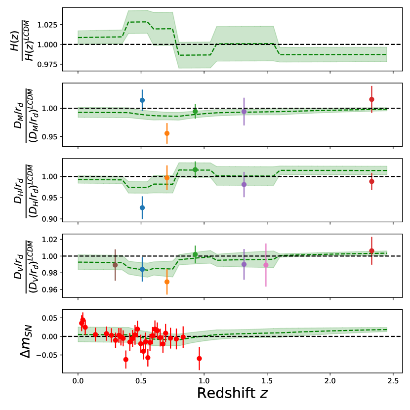
Figure 1: Constraints from our modified-H model, assuming DESI+CMB+DESY5 data. We show the constraints on the expansion rate $H(z)$ (top panel), followed (in panels that follow, moving down) by the derived constraints on the angular-diameter distance, Hubble distance, and volume-averaged distance all divided by the sound horizon, and finally the apparent magnitude of SNIa. All of the quantities are shown relative to their $\Lambda$CDM values computed with best-fit parameters from our analysis. The data points show the DESI Y1 BAO measurements, except in the lowest panel where we show data from SNIa. See text for more details, and in particular the explanation of how SNIa magnitude residuals were defined.

IV Results

The constraints on the six alpha parameters from the DESI+CMB+DESY5 analysis, marginalized over the baryon and CDM number densities and the Hubble constant, are shown in Fig. 6 in Appendix B, while the corresponding parameter constraints are shown in Table 2 in that Appendix. Overall, we find that the modified-H model gives a slightly better fit to the data than the $(w_{0},w_{a})$ model — not nearly better enough to indicate a preference for our more complex model, but sufficiently so to indicate that the model is a good fit to the data Overall, the alpha parameters are consistent with zero values predicted by $\Lambda$CDM, though we observe a modest 2$\sigma$ deviation from zero in the second alpha parameter.

A more detailed picture can be obtained by looking at the derived constraints on the Hubble parameter and distances, shown in Fig. 1 for the DESI+CMB+DESY5 data combination. We show, from top to bottom, the derived Hubble parameter; the corresponding constraints on the angular-diameter, Hubble, and volume-averaged distance; and finally the constraint on the apparent magnitude of SNIa, all as a function of redshift. In all cases, we show constraints relative to their $\Lambda$CDM values computed with best-fit parameters from our analysis (i.e. best-fit $H_{0}^{\rm LCDM}$ and $\Omega_{\mathrm{m}}$, effectively); the $\Lambda$CDM best-fit values are shown as black dashed lines and centered respectively at either 1 or zero Note the general agreement of the predictions from our modified-H model with those from $\Lambda$CDM. The most noticeable discrepancy between the two is a 3-5% "bump" in the expansion rate at $z\simeq 0.5$, which integrates to contribute to a trough in the distances as $z\simeq 1$.

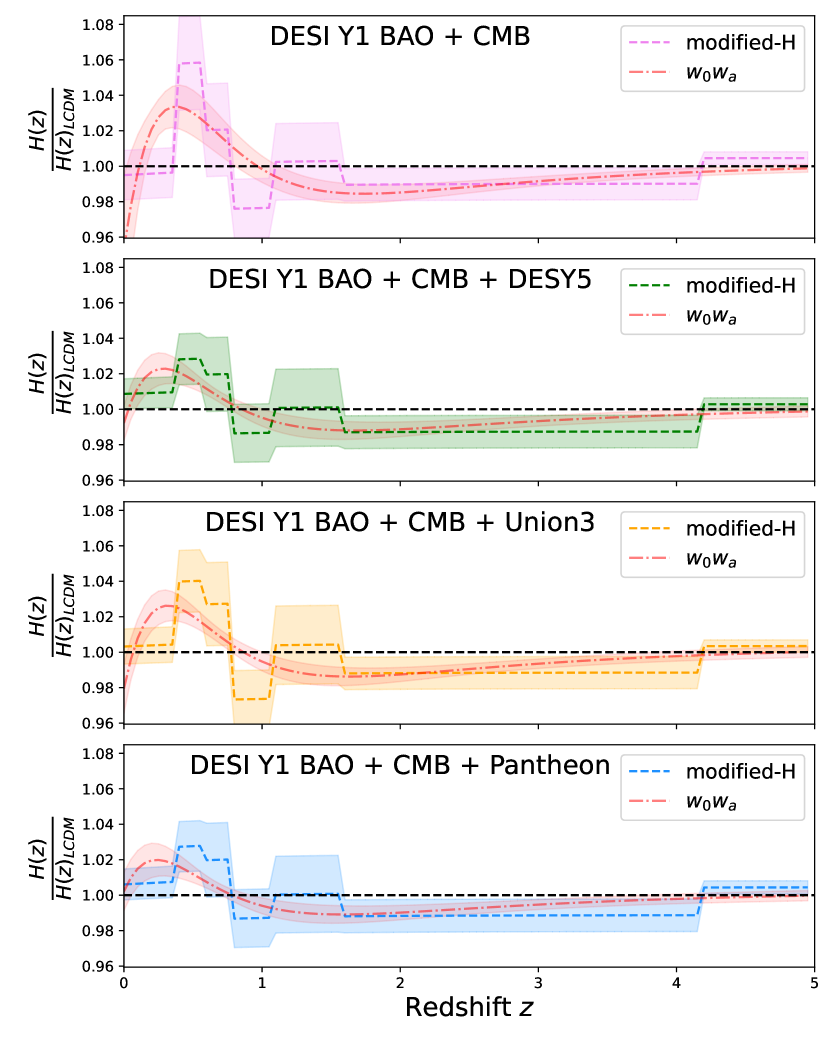
Figure 2: A more detailed view of the $H(z)$ constraint relative to its best-fit value in $\Lambda$CDM. We show constraints from DESI BAO and CMB in the first panel (without supernovae), followed by the constraints including one of the three SNIa datasets (DESY5, Union3, and PantheonPlus, respectively in the second, third, and fourth panels). In each case we show comparison with the corresponding best-fit constraint that assumes the ($w_{0},w_{a}$) model.

Figure 2 focuses attention on the preferences in the expansion rate provided by the DESI+CMB and DESI+CMB+SNIa data in our modified-H model. Here, we present the expansion rate relative to that of the best-fit $\Lambda$CDM model for the combination of DESI Y1 BAO and CMB alone, and also DESI and CMB combined with either one of the three SNIa datasets: DESY5, Union3, and PantheonPlus (so the second panel of Fig. 2 has the same information as the top panel in Fig. 1). We compare our results with those from the ($w_{0},w_{a}$) parameterization, shown as the red contours in Fig. 2. The preferences from the modified-H model show excellent overall agreement with those from the ($w_{0},w_{a}$) parameterization, both for the DESI BAO+CMB combination and for the combinations that include supernovae datasets (DESI BAO+CMB+SNIa): both models show preference for the aforementioned $\sim$3-5% bump in the expansion rate at $z\simeq 0.5$. This bump is not particularly significant (being 2.2$\sigma$ for the DESI BAO + CMB combination, and 2.0$\sigma$, 2.3$\sigma$, and 2.3$\sigma$ respectively for combinations of DESI and CMB with DESY5, Union3, and PantheonPlus), but it importantly agrees with the same feature in ($w_{0},w_{a}$) model which does not have the flexibility to cleanly isolate this feature but does have more statistical power due to having fewer parameters. Further, both the modified-H and ($w_{0},w_{a}$) model show a very mild ($\sim$1$\sigma$) preference for a lower-than-Lambda $H(z)$ at $z\gtrsim 1.5$.

The late-time increase in the expansion rate, if confirmed by future data, would correspond to the corresponding increase in the dark-energy density. Roughly speaking, such an increase could be caused by "thawing" scalar field [42] that starts to evolve at late times ($z\lesssim 1$) and thus has an equation of state $w(z)>-1$ and a correspondingly higher density than that in vacuum energy. We do not pursue comparisons with specific dark-energy models further.

One particularly interesting and, to our knowledge, novel result is that all four data combinations shown in Fig. 2 favor the model where $H(z)$ agrees with the $\Lambda$CDM prediction (anchored at high redshift) even at very low redshift, as $z\rightarrow 0$. The ($w_{0},w_{a}$) parameterization does not allow such a variation, since $H(z)$ is affected by a change in $w$ only at first order in $z$ (and comoving distance at second order) [43]; in other words, the value of $H(z=0)$ is completely determined by values of $H_{0}^{\rm LCDM}$ and $\Omega_{\mathrm{m}}$ anchored at high redshift in both $\Lambda$CDM and $w_{0}w_{a}$CDM model. In contrast, our parameterization allows a more abrupt, zeroth-order in redshift change in $H(z)$. This in principle allows the disagreement between $H(z\rightarrow 0)$ and $H_{0}^{\rm LCDM}$ in the modified-H model, which the data however do not prefer. It is tantalizing to consider implications of this internal concordance test for direct Hubble-constant measurements that use the astronomical distance ladder, but that will require an in-depth investigation that we leave for near-future work.

Finally, we note that we have done internal checks by changing the details of the binning. We found some dependence of the $\Delta\chi^{2}$ values on the choice of the binning, but overall results that are consistent with those presented here.

V Conclusions

Our principal goal, with the flexible modeling of the expansion history and dark-energy sector given in our Eq. (1), was to give a somewhat more nuanced conclusions on dark energy than constraints from simple parameterizations of the equation of state of dark energy. Assuming the combination of DESI Y1 BAO, compressed Planck and ACT, and SNIa data, we find results remarkably consistent with those from the popular ($w_{0},w_{a}$) model. We observe a mild preference for the $\sim$3-5% "bump" in the expansion rate at $z\simeq 0.5$ relative to the fit of $\Lambda$CDM model to the same data, and a general agreement with findings from $\Lambda$CDM at higher redshift. Moreover, even though we allow variations in the expansion rate at low redshift relative to $H(z)$ anchored at high redshift, we see no evidence for the departure from $\Lambda$CDM model’s expectation as $z\rightarrow 0$.

One might be tempted to criticize our modified-H model as insufficiently "physical", as it allows for sharp transitions in the expansion rate. We think that our model’s flexibility, especially one that goes beyond that of smooth $w(z)$ descriptions, is precisely its feature. Given the lack of any compelling dark-energy models, it is essential to keep an open mind regarding the description of the dark-energy sector. That is what we have proceeded to do here.

Finally, we have also provided in Appendix A an accurate compression of the CMB (Planck+ACT) data, which should prove useful in constraining beyond-standard models of dark energy.

It is becoming clear that a relatively low redshift range, $z\lesssim 0.8$, is becoming very interesting to explore with future and better data. This is where we (with the modified-H model) and previous findings (with the ($w_{0},w_{a}$) parameterization) consistently see hints of a preference for dynamical dark energy, although this could certainly be just a statistical fluctuation. This is also the redshift range where we rely in good measure to data from SNIa, which are essential in predicting the behavior of dark energy at $z\lesssim 1$. It is precisely at these relatively low redshifts where additional BAO data will be extremely useful.

Acknowledgments. This work has been supported by the Department of Energy under contract DE-SC0019193. We thank our many collaborators on the DESI analysis team for discussions that have influenced our thinking about the implications of DESI dark-energy results.

Appendix A Validation of the CMB compression

Here we provide more details on the validation of our compressed CMB datavector and its covariance shown in Eqs. (5)-(6).

We obtain the aforementioned compression by considering the joint likelihood that makes use of the PR3 Planck plik likelihood [36] likelihood [44] and the Data Release 6 of ACT [37]. We next run the Monte Carlo Markov Chain (MCMC) sampler Cobaya [24] on these data. We compute the three-dimensional compressed data-vector and its covariance by running Cobaya on the $\Lambda$CDM model. Then, for our validation tests, we use the actual $\Lambda$CDM constraints from the aforementioned analysis, and also run Cobaya on the $w_{0}w_{a}$CDM model to get constraints in that parameter space.

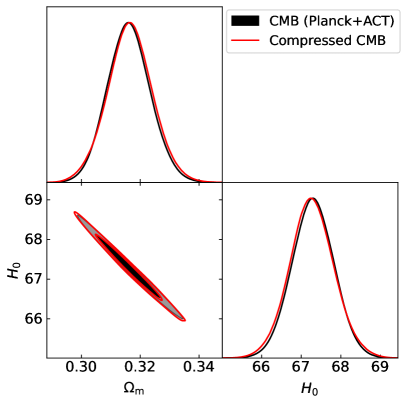
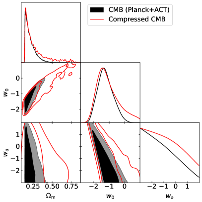
Figure 3: Comparison of full CMB constraints to those from the compressed CMB datavector in the $\Lambda$CDM model (left panel) and $w_{0}w_{a}$CDM model (right panel). Black lines and filled contours show the constraint from the full Planck (2018) + ACT (DR6) chain, while the red lines and open contours show the approximate constraints from our compressed data-vector.

For our MCMC chains, we use the default convergence criteria of Gelman and Rubin R statistic $<$ 0.01. To calculate the means, confidence intervals and likelihood distributions for our model parameters, we use GetDist [25] code with our converged MCMC chains.

Figure 3 shows the comparison of the constraints from the CMB and those derived from our compressed datavector in two cosmological models. In the left panel, we show constraints in $\Lambda$CDM  with the matter density relative to critical $\Omega_{\mathrm{m}}$ and the Hubble constant $H_{0}$ as the only free parameters. The agreement between the full Planck (2018)+ACT (DR6) likelihood is excellent, though mostly by construction since our compressed quantities are derived from the $\Lambda$CDM MCMC analysis.

A much more convincing validation is obtained with a comparison to another model on which the datavector was not explicitly trained. We adopt the popular phenomenological model that models the equation of state of dark energy as $w(a)=w_{0}+w_{a}(1-a)$, where $a$ is the scale factor and $w_{0}$ and $w_{a}$ are two free parameters. In the right panel of Fig. 3 we compare constraints on the parameter space $(\Omega_{\mathrm{m}},w_{0},w_{a})$ from the full CMB chain and those derived with our compressed datavector. The agreement is now visually less good, especially in $w_{a}$, but note that the principal features of the CMB constraint in this very degenerate parameter space are still reasonably well recovered with the compressed analysis. This bodes well for more realistic cosmological analyses when various datasets will be combined with the CMB in parameter spaces that would be very poorly determined by the CMB alone.

To test this conjectured increased robustness with data of increased constraining strength, we combine the same CMB data (Planck (2018) + ACT (DR6)) with the BAO data from the first year of Dark Energy Spectroscopic Instrument (DESI Y1 BAO) [1]. The left panel of Fig. 4 shows the expected good agreement between the exact and approximate treatment in $\Lambda$CDM. The right panel, in turn, shows encouraging results from a much less trivial comparison in the $w_{0}w_{a}$CDM model (on which, recall, the compression was not explicitly trained). We see an excellent agreement between the combined DESI Y1 BAO + CMB results, down to tracing subtle non-Gaussianities in the 2D parameter posteriors.

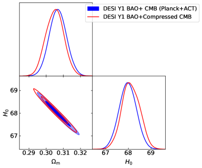
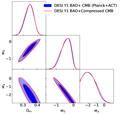
Figure 4: Comparison of the combined CMB and DESI Y1 BAO constraints in the $\Lambda$CDM model (left panel) and the $w_{0}w_{a}$CDM model (right panel) to those obtained when the CMB likelihood is replaced with the compressed datavector and its covariance. The blue lines and filled contours show the constraints when we use the full Planck + ACT chains for the CMB, while the red lines and open contours show the results with our compressed CMB datavector.

The results just shown indicate that our compressed datavector faithfully represents the CMB information in cases when non-standard models affect the expansion history, as e.g. in the $w_{0}w_{a}$CDM model.

When computing the compressed CMB datavector and covariance, we fixed the redshift $z_{*}$ (photon decoupling surface) to $1090$ to calculate the means and covariances using the CAMB [45] software. It is natural to question the validity of this assumption, as $z_{*}$ depends on the expansion history, and hence on the dark-energy model [46]. To address this issue, we recomputed the means and covariances using CAMB without fixing $z_{*}$. The derived quantities, rstar and DAstar, were calculated directly from CAMB and used to compute $R$ and $\ell_{a}$. Figure 5 compares the constraints obtained using the two approaches for both the $\Lambda$CDM and $w_{0}w_{a}$CDM cases. Some references [47, 48, 49] have suggested using the approximate expression for $z_{*}$ from Hu & Sugiyama [46] for the compressed CMB likelihood. However, these expressions cannot be applied to exotic models that affect the thermal history of the universe. In such cases, our compression proves particularly useful, as it only requires computing the background quantities at $z_{*}=1090$ without any additional thermal history calculations to correct $z_{*}$.

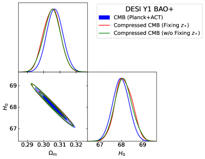
Figure 5: Comparison of the combined CMB and DESI Y1 BAO constraints in the $\Lambda$CDM model (left panel) and the $w_{0}w_{a}$CDM model (right panel). The blue lines and filled contours show the constraints when we use the full Planck + ACT chains for the CMB, while the red lines and open contours show the results with our compressed CMB datavector.

Appendix B Constraints on the alphas

Here we provide more detailed information about the constraints on the alpha parameters defined in our modified-H model (see Eq. (1)). Figure 6 shows the constraints on the six alpha parameters, marginalized over the three remaining parameters ($\Omega_{\mathrm{b}}h^{2},\Omega_{\mathrm{cdm}}h^{2}$ and $H_{0}^{\rm LCDM}$), assuming DESI+CMB+DESY5 data, while Table 2 shows the numerical constraints on all parameters. We see that each of the six alphas is constrained reasonably well; the errors are ballpark $0.01$ to $0.04$, and this is how well the fractional expansion rate is constrained in the respective redshift bins. Note also that we iterated a little in selecting our flat priors on the alphas in order to ensure that none of the constraints hits the prior boundaries. Table 2 shows the numerical constraints on all eight parameters of our model, also assuming DESI+CMB+DESY5 data. [For clarity we do not show the constraints with the Union3 or PantheonPlus SNIa datasets.]

Table 2: Constraints on the fundamental parameters of our modified-H model in our fiducial analysis of DESI+CMB+DESY5.

Parameter	Constraint
$H_{0}^{\rm LCDM}$   (value adopted from $\Lambda$CDM fit)	$67.76$ (Fixed)
$\Omega_{\mathrm{b}}h^{2}$	$0.02239\pm 0.00014$
$\Omega_{\mathrm{cdm}}h^{2}$	$0.1200\pm 0.0011$
$\alpha_{1}$	$0.0086\pm 0.0085$
$\alpha_{2}$	$0.027\pm 0.014$
$\alpha_{3}$	$0.018\pm 0.021$
$\alpha_{4}$	$-0.015\pm 0.016$
$\alpha_{5}$	$-0.001\pm 0.022$
$\alpha_{6}$	$-0.015\pm 0.010$

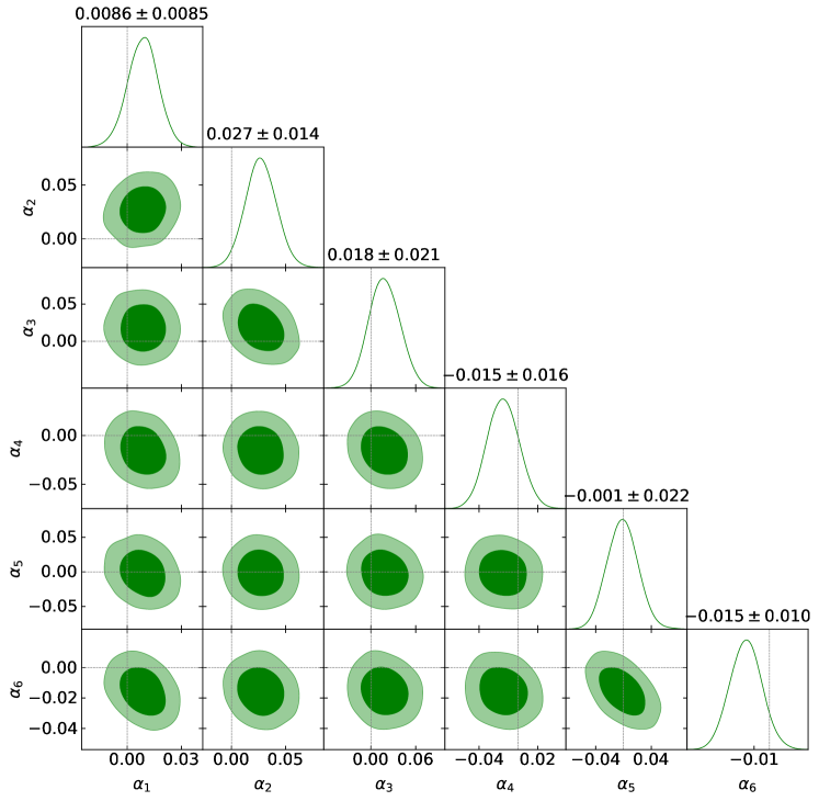
Figure 6: Constraints on the six parameters that describe perturbations in the Hubble rate (see Eq. 1), marginalized over the three remaining parameters ($\Omega_{\mathrm{b}}h^{2},\Omega_{\mathrm{cdm}}h^{2}$ and $H_{0}^{\rm LCDM}$). The contours represent the 68.3% and 95.4% credible regions, and the numbers above each diagonal panel shows the projected mean and error in the corresponding alpha. The faint dashed lines are centered at fiducial values in the $\Lambda$CDM model, which is zero for each of the alphas.

Appendix C Neutrino Density

We have accounted for the neutrino density using the formalism developed in WMAP 7-year analysis [50]

$$\Omega_{\nu}(a)=0.2271\Omega_{\gamma}(a)N_{\mathrm{eff}}\left(\frac{1}{3}\sum_{i=1}^{3}f(m_{\nu,i}a/T_{\nu,0})\right)\,.$$ (7)

Here $N_{\mathrm{eff}}$ is the effective number of neutrino species (fixed at a value 3.044 for this analysis), $a$ is the scale factor, $\Omega_{\gamma}$ is the photon density and $T_{\nu,0}$ is the neutrnio temperature at $z=0$ ($a=1$) given by

$$T_{\nu,0}=\left(\frac{4}{11}\right)^{1/3}T_{\mathrm{CMB}}=1.945\mathrm{K}\,.$$ (8)

The function $f$ represents the Fermi-Dirac integral given by

$$f(y)=\frac{120}{7\pi^{4}}\int_{0}^{\infty}\frac{x^{2}\sqrt{x^{2}+y^{2}}}{e^{x}+1}.$$ (9)

To make the code more efficient, we have used the fitting formula [50]

$$f(y)\approx(1+(Ay)^{p})^{1/p}$$ (10)

where $A\approx 0.3173$ and $p=1.83$.

For the case of two massless neutrinos and one massive neutrino of mass $m_{\nu}=0.06$ $\mathrm{eV}$, the term in the paranthesis in Eq. (7) simplifies to

$$\frac{1}{3}(2+f(m_{\nu}a/T_{\nu,0}))\,.$$ (11)

Combining Eq. (7) with the photon density, we can write the total radiation density (including the contribution from massive neutrinos) as

$$\Omega_{\mathrm{R}}(a)=\Omega_{\gamma}(a)+\Omega_{\nu}(a)$$ (12)

References

- Adame et al. [2024a] A. G. Adame et al. (DESI), (2024a), arXiv:2404.03002 [astro-ph.CO] .
- Aghamousa et al. [2016] A. Aghamousa et al. (DESI), (2016), arXiv:1611.00036 [astro-ph.IM] .
- Abareshi et al. [2022] B. Abareshi et al. (DESI), Astron. J. 164, 207 (2022), arXiv:2205.10939 [astro-ph.IM] .
- Linder [2003] E. V. Linder, Phys. Rev. Lett. 90, 091301 (2003), arXiv:astro-ph/0208512 .
- Chevallier and Polarski [2001] M. Chevallier and D. Polarski, Int. J. Mod. Phys. D 10, 213 (2001), arXiv:gr-qc/0009008 .
- Lodha et al. [2024] K. Lodha et al. (DESI), (2024), arXiv:2405.13588 [astro-ph.CO] .
- Calderon et al. [2024] R. Calderon et al. (DESI), JCAP 10, 048, arXiv:2405.04216 [astro-ph.CO] .
- Mukherjee and Sen [2024] P. Mukherjee and A. A. Sen, Phys. Rev. D 110, 123502 (2024), arXiv:2405.19178 [astro-ph.CO] .
- Dinda and Maartens [2025] B. R. Dinda and R. Maartens, JCAP 01, 120, arXiv:2407.17252 [astro-ph.CO] .
- Rebouças et al. [2024] J. a. Rebouças, D. H. F. de Souza, K. Zhong, V. Miranda, and R. Rosenfeld, (2024), arXiv:2408.14628 [astro-ph.CO] .
- Ishak et al. [2024] M. Ishak et al., (2024), arXiv:2411.12026 [astro-ph.CO] .
- Chudaykin and Kunz [2024] A. Chudaykin and M. Kunz, Phys. Rev. D 110, 123524 (2024), arXiv:2407.02558 [astro-ph.CO] .
- Green and Meyers [2024] D. Green and J. Meyers, (2024), arXiv:2407.07878 [astro-ph.CO] .
- Elbers et al. [2024] W. Elbers, C. S. Frenk, A. Jenkins, B. Li, and S. Pascoli, (2024), arXiv:2407.10965 [astro-ph.CO] .
- Cortês and Liddle [2024] M. Cortês and A. R. Liddle, JCAP 12, 007, arXiv:2404.08056 [astro-ph.CO] .
- Berghaus et al. [2024] K. V. Berghaus, J. A. Kable, and V. Miranda, Phys. Rev. D 110, 103524 (2024), arXiv:2404.14341 [astro-ph.CO] .
- Park et al. [2024a] C.-G. Park, J. de Cruz Pérez, and B. Ratra, Phys. Rev. D 110, 123533 (2024a), arXiv:2405.00502 [astro-ph.CO] .
- Poulin et al. [2024] V. Poulin, T. L. Smith, R. Calderón, and T. Simon, (2024), arXiv:2407.18292 [astro-ph.CO] .
- Jiang et al. [2024] J.-Q. Jiang, D. Pedrotti, S. S. da Costa, and S. Vagnozzi, Phys. Rev. D 110, 123519 (2024), arXiv:2408.02365 [astro-ph.CO] .
- Wolf et al. [2024] W. J. Wolf, C. García-García, D. J. Bartlett, and P. G. Ferreira, Phys. Rev. D 110, 083528 (2024), arXiv:2408.17318 [astro-ph.CO] .
- Park et al. [2024b] C.-G. Park, J. de Cruz Perez, and B. Ratra, (2024b), arXiv:2410.13627 [astro-ph.CO] .
- Linder [2024] E. V. Linder, (2024), arXiv:2410.10981 [astro-ph.CO] .
- Lewis and Chamberlain [2024] A. Lewis and E. Chamberlain, (2024), arXiv:2412.13894 [astro-ph.CO] .
- Torrado and Lewis [2021] J. Torrado and A. Lewis, JCAP 05, 057, arXiv:2005.05290 [astro-ph.IM] .
- Lewis [2019] A. Lewis, (2019), arXiv:1910.13970 [astro-ph.IM] .
- Adame et al. [2024b] A. G. Adame et al. (DESI), (2024b), arXiv:2404.03000 [astro-ph.CO] .
- Adame et al. [2025] A. G. Adame et al. (DESI), JCAP 01, 124, arXiv:2404.03001 [astro-ph.CO] .
- Adame et al. [2024c] A. G. Adame et al. (DESI), (2024c), arXiv:2411.12022 [astro-ph.CO] .
- Bond et al. [1997] J. R. Bond, G. Efstathiou, and M. Tegmark, Mon. Not. Roy. Astron. Soc. 291, L33 (1997), arXiv:astro-ph/9702100 .
- Wang and Mukherjee [2007] Y. Wang and P. Mukherjee, Phys. Rev. D 76, 103533 (2007), arXiv:astro-ph/0703780 .
- Elgaroy and Multamaki [2007] O. Elgaroy and T. Multamaki, Astron. Astrophys. 471, 65 (2007), arXiv:astro-ph/0702343 .
- Komatsu et al. [2011a] E. Komatsu et al. (WMAP), Astrophys. J. Suppl. 192, 18 (2011a), arXiv:1001.4538 [astro-ph.CO] .
- Vonlanthen et al. [2010] M. Vonlanthen, S. Räsänen, and R. Durrer, JCAP 08, 023, arXiv:1003.0810 [astro-ph.CO] .
- Huang et al. [2015] Q.-G. Huang, K. Wang, and S. Wang, JCAP 12, 022, arXiv:1509.00969 [astro-ph.CO] .
- Zhai et al. [2020] Z. Zhai et al., JCAP 07, 009, arXiv:1912.04921 [astro-ph.CO] .
- Aghanim et al. [2020] N. Aghanim et al. (Planck), Astron. Astrophys. 641, A5 (2020), arXiv:1907.12875 [astro-ph.CO] .
- Madhavacheril et al. [2024] M. S. Madhavacheril et al. (ACT), Astrophys. J. 962, 113 (2024), arXiv:2304.05203 [astro-ph.CO] .
- Abbott et al. [2024] T. M. C. Abbott et al. (DES), Astrophys. J. Lett. 973, L14 (2024), arXiv:2401.02929 [astro-ph.CO] .
- Rubin et al. [2023] D. Rubin et al., (2023), arXiv:2311.12098 [astro-ph.CO] .
- Scolnic et al. [2022] D. Scolnic et al., Astrophys. J. 938, 113 (2022), arXiv:2112.03863 [astro-ph.CO] .
- Peterson et al. [2022] E. R. Peterson et al., Astrophys. J. 938, 112 (2022), arXiv:2110.03487 [astro-ph.CO] .
- Caldwell and Linder [2005] R. R. Caldwell and E. V. Linder, Phys. Rev. Lett. 95, 141301 (2005), arXiv:astro-ph/0505494 .
- Huterer and Turner [2001] D. Huterer and M. S. Turner, Phys. Rev. D 64, 123527 (2001), arXiv:astro-ph/0012510 .
- Carron et al. [2022] J. Carron, M. Mirmelstein, and A. Lewis, JCAP 09, 039, arXiv:2206.07773 [astro-ph.CO] .
- Lewis et al. [2000] A. Lewis, A. Challinor, and A. Lasenby, ApJ 538, 473 (2000), arXiv:astro-ph/9911177 [astro-ph] .
- Hu and Sugiyama [1996] W. Hu and N. Sugiyama, The Astrophysical Journal 471, 542–570 (1996).
- Gao et al. [2024] Q. Gao, Z. Peng, S. Gao, and Y. Gong, (2024), arXiv:2411.16046 [astro-ph.CO] .
- Liu et al. [2024] G. Liu, Y. Wang, and W. Zhao, Phys. Lett. B 854, 138717 (2024), arXiv:2401.10571 [astro-ph.CO] .
- Lazkoz et al. [2024] R. Lazkoz, V. Salzano, L. Fernandez-Jambrina, and M. Bouhmadi-López, Phys. Dark Univ. 45, 101511 (2024), arXiv:2311.10526 [astro-ph.CO] .
- Komatsu et al. [2011b] E. Komatsu et al., The Astrophysical Journal Supplement Series 192, 18 (2011b).