Efficient classical error correction for parity-encoded spin systems

Abstract

Fast solvers for combinatorial optimization problems (COPs) have garnered engineering interest across various industrial and social applications. Quantum annealing (QA) has emerged as a promising candidate, with considerable efforts dedicated to its development. Since COP is encoded in the Ising interaction among logical spins, its realization necessitates a spin system with all-to-all connectivity, presenting technical challenges in the physical implementation of large-scale QA devices. W. Lechner, P. Hauke, and P. Zoller proposed a parity-encoding (PE) architecture, which consists of an enlarged system of physical spins with only local connectivity among them, to circumvent this difficulty in developing near-future QA devices. They suggested that this architecture not only alleviates implementation challenges and enhances scalability but also possesses intrinsic fault tolerance, as logical spins are redundantly and nonlocally encoded in the physical spins. Nevertheless, it remains unclear how these advantageous features can be exploited. This paper addresses correcting errors in a spin readout of PE architecture. Our work is based on the close connection between PE architecture and classical low-density parity-check (LDPC) codes. We have shown that independent and identically distributed errors in a spin readout can be corrected using a straightforward decoding algorithm that can be viewed as a bit flipping (BF) algorithm for the LDPC codes. The BF algorithm has been shown to perform comparably to the belief propagation (BP) decoding algorithm. Furthermore, it is suggested that the introduction of post-readout BF decoding reduces the total computational cost and enhances the performance of the global optimal solution search using the PE architecture. Our results indicate that the PE architecture is a promising platform for near-term QA devices.

I Introduction

Combinatorial optimization problems (COPs) present significant mathematical challenges in various industrial applications, including routing, scheduling, planning, decision-making, transportation, and telecommunications. COPs have garnered the attention of many researchers, leading to intensive efforts to develop a fast solver for these problems. Since many COPs are NP-hard, effective approximation methods such as heuristics Pearl (1984) and meta-heuristics Peres and Castelli (2021), have often been employed to tackle related challenges. Computational models of natural phenomena inspire some of these methods and rely on probabilistic simulations of dynamic processes in physical systems. They can be executed on digital computers or specially designed physical hardware. Recently, there has been increasing interest in natural computing, with new nature-inspired computing hardware being proposed and analyzed based on intriguing natural systems such as neural networks, molecules, DNA, and quantum computers Jiao et al. (2024).

There is a growing interest in quantum annealing (QA) devices as fast solver candidates for COP Heng et al. (2022). The COPs can be mapped to a search for the ground state of the Hamiltonian of the Ising spin network. The QA device is designed to search for such ground states quickly by exploiting quantum phenomena. Various architectures of QA devices have been developed to solve large-scale industrial and social optimization problems in a reasonable amount of time. D-Wave Systems was the first to create a commercial QA device consisting of superconducting flux qubits Johnson et al. (2011); King et al. (2021); Raymond et al. (2023); King et al. (2023, 2022). Another QA device, called a coherent Ising machine, has been developed using optical systems. Wang et al. (2013); Marandi et al. (2014); McMahon et al. (2016); Inagaki et al. (2016). Kerr parametric oscillators (KPOs) have been proposed as alternative candidates for components of a QA device. Goto (2016); Nigg et al. (2017); Puri et al. (2017); Zhao et al. (2018); Goto (2019); Onodera et al. (2020); Goto and Kanao (2020); Kewming et al. (2020); Kanao and Goto (2021); Yamaji et al. (2023).

To universally apply QA devices to a COP, simulating a fully connected graph model with an Ising spin network is essential. This requirement is technically demanding, especially in implementing QA devices using superconducting and semiconductor technology, as long-range interactions between spins must be established. To circumvent this problem, a network of logical spins with long-range interactions is usually embedded in an enlarged network of physical spins that exhibit only short-range interactions. Minor embedding techniques can replace logical spins with long-range interactions by physical spins with short-range interactions among ferromagnetically coupled chains of spins Choi (2008, 2011). W. Lechner, P. Hauke, and P. Zoller (LHZ) independently proposed a scalable embedding scheme called the parity-encoding (PE) architecture. Lechner et al. (2015). Overhead comes at the cost of these embedding schemes, as the results of successive short-range interactions simulate long-range interactions. On the other hand, LHZ suggested that the PE architecture has a notable feature of intrinsic fault tolerance. This suggestion is also supported by F. Pastawski and J. Preskill (PP) Pastawski and Preskill (2016). They pointed out that the PE architecture is interpreted as a classical low-density parity-check (LDPC) code Gallager (1962, 1963) and demonstrated that if the errors are independent and identically distributed (i.i.d.), the spin readout errors can be corrected through appropriate decoding. PP utilized the belief propagation (BP) algorithm, recognized as the standard decoding algorithm for classical LDPC codes Pearl (1982), to correct spin readout errors in the PE architecture. T. Albash, W. Vincl, and D. Lidar discussed decoding algorithms based on various strategies, including a simple majority voting strategy Albash et al. (2016). They reported that PE architectures do not necessarily exhibit intrinsic fault tolerance. They speculated that the discrepancy with fault-tolerance claims arose because a model of weakly correlated spin-flip errors cannot accurately describe errors caused by dynamic or thermal excitations during QA evolution. This contradiction remains unresolved, and whether the fault tolerance inherent in the PE architecture can be exploited is unclear.

Motivated by previous studies, this paper examines how errors in the readout of PE architectures can be corrected. Our study is based on the close connection between the PE architecture and the classical LDPC codes noted by PP. We demonstrate that the spin system initially proposed by Sourlas Sourlas (2005) and later by LHZ (referred to as the SLHZ system) is a realization of the PE architecture, and COP based on the Hamiltonian of the SLHZ system is equivalent to decoding the LDPC codes. We propose an iterative hard decision decoding algorithm based on majority voting in a generalized syndrome, known as Gallager’s bit flipping (BF) algorithm within the context of LDPC codes Gallager (1962, 1963). Assuming the i.i.d. noise model, we demonstrate that the BF decoding algorithm can correct spin readout errors with performance comparable to that of the BP algorithm.

To test the performance of the BF decoder as a post-readout decoder for the SLHZ system, a classical Markov chain Monte Carlo (MCMC) sampler was employed to simulate the stochastically sampled readouts of spins in the SLHZ system. We present evidence that the BF decoding algorithm, similar to the BP decoding algorithm, can correct errors in the simulated readouts of SLHZ systems. The simulation results show that applying BF decoding to the readouts from the MCMC sampler reduces the overall decoding costs. Our findings suggest that a hybrid approach combining two different types of decoding algorithms, MCMC decoding and BF decoding, can be utilized to reduce the overhead inherent in SLHZ systems. We sought to understand this phenomenon by comparing our algorithm with various known BF decoding algorithms. Although the current results are based on classical simulations, the main points discussed in this study apply to both classical MCMC samplers and quantum annealing (QA) devices, and we believe that the SLHZ system is a promising candidate for the realization of near-term QA devices.

This paper is organized as follows. Sec.II briefly explains error-correcting codes (ECC) and probabilistic decoding as a preliminary step. Section III describes the connection between LDPC codes and SLHZ systems, and proposes a simple BF decoding algorithm for SLHZ systems. Section IV demonstrates the performance of the proposed BF decoding in correcting errors in the readout of the SLHZ system. In Sec.V, we outline several types of BF decoding algorithms and their relation to our algorithm. We explain why two-stage hybrid decoding performs better than either of the two algorithms individually. Sec.VI concludes this paper.

II Preliminaries

II.1 Model

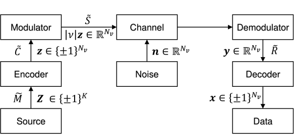
Figure 1: A considered model for a communication system.

First, let’s describe our model. A binary source-word $\tilde{M}$ is first encoded into a binary code-word $\tilde{C}$ using ECC. The code-word is then modulated into the real signal $\tilde{S}$ and transmitted. During transmission, the signal is affected by noise in a transmission channel. At the end of the channel, the received signal is demodulated to obtain the observations $\tilde{R}$ (Fig.1). The ECC aims to communicate reliably over a noisy channel. Let $\tilde{M}$ and $\tilde{C}$ be $K$ bits and $N_{v}\left(>K\right)$ bits, respectively, and denote them by the binary vectors $\boldsymbol{\bar{Z}}=\left(\bar{Z}_{1},\ldots,\bar{Z}_{K}\right)\in\left\{0,1\right\}^{K}$ and $\bar{\boldsymbol{z}}=\left(\bar{z}_{1},\ldots,\bar{z}_{N_{v}}\right)\in\left\{0,1\right\}^{N_{v}}$, respectively. A Linear code is defined by a one-to-one map from $\tilde{M}$ in the set $\left\{\bar{\boldsymbol{Z}}\right\}$ of $2^{K}$ source-words $\tilde{M}$ of length $K$ to $\tilde{C}$ in the set $\left\{\bar{\boldsymbol{z}}\right\}$ of $2^{K}$ code-words $\tilde{C}$ of length $N_{v}$. They are specified by a generating matrix $\boldsymbol{G}_{K\times N_{v}}$ or a generalized parity check matrix $\boldsymbol{H}_{N_{c}\times N_{v}}$ satisfying $\boldsymbol{G}\boldsymbol{H}^{T}=\boldsymbol{0}_{K\times N_{c}}\>\left(\mathrm{mod}\>2\right)$. Here $\boldsymbol{G}$ and $\boldsymbol{H}$ are binary matrices (i.e., their elements are 0 or 1) and “$\mathrm{mod}\>2$” denotes that the multiplication is modulo two. The source-word $\boldsymbol{\bar{Z}}$ is mapped to the code-word $\bar{\boldsymbol{z}}$ by $\bar{\boldsymbol{z}}=\boldsymbol{\bar{Z}}\boldsymbol{G}\>\left(\mathrm{mod}\>2\right)$. Note that any $K$ linearly independent code-words can be used to form the generating matrix. For an arbitrary $N_{v}$-dimensional vector $\boldsymbol{\bar{x}}=\left(\bar{x}_{1},\ldots,\bar{x}_{N_{v}}\right)\in\left\{0,1\right\}^{N_{v}}$, define the generalized syndrome vector $\boldsymbol{\bar{s}}\left(\boldsymbol{\bar{x}}\right)=\left(\bar{s}_{1}\left(\boldsymbol{\bar{x}}\right),\ldots,\bar{s}_{N_{c}}\left(\boldsymbol{\bar{x}}\right)\right)$ (generalized because it may not have $N_{v}-K$ bits) as $\boldsymbol{\bar{s}}\left(\boldsymbol{\bar{x}}\right)=\bar{\boldsymbol{x}}\boldsymbol{H}^{T}\>\left(\mathrm{mod}\>2\right)$. Then, $\bar{\boldsymbol{x}}$ is a code-word if and only if $\boldsymbol{\bar{s}}\left(\boldsymbol{\bar{x}}\right)=\boldsymbol{0}_{1\times N_{c}}$. This defines a set of equations called the generalized parity check equations. Note that they consist of a set of $N_{c}$ equations but only $N_{v}-K$ of which are linearly independent. It follows that the parity-check matrix for a given linear code can be chosen in many ways and that many syndrome vectors can be defined for the same code. The ratio of the length of the source-word to that of the code-word is called the rate: $r=K/N_{v}$. Later in this section, we will show specific examples of the matrices $\boldsymbol{G}$ and $\boldsymbol{H}$ for the PE architecture. The code-word $\bar{\boldsymbol{z}}$ is converted into a sequence of bipolar variables $\boldsymbol{z}=\left(z_{1},\ldots,z_{N_{v}}\right)\in\left\{\pm 1\right\}^{N_{v}}$ ($0$ is mapped to $+1$, and $1$ to $-1$) and modulated to antipodal signals $\left|v\right|\boldsymbol{z}$ by a binary phase shift keying modulation, where $\left|v\right|$ is signal amplitude. Assume that the signal $\tilde{S}$ is transmitted over a channel having additive white Gaussian noise (AWGN). At the end of the channel, the receiver obtains an observation $\tilde{R}$, denoted by an antipodal vector $\boldsymbol{y}=\left(y_{1},\ldots,y_{N_{v}}\right)=\left|v\right|\boldsymbol{z}+\boldsymbol{n}\in\mathbb{R}^{N_{v}}$ where $\boldsymbol{n}=\left(n_{1},\ldots,n_{N_{v}}\right)\in\mathbb{R}^{N_{v}}$ is noise vector whose elements are i.i.d. Gaussian random variables with zero mean and variance $\sigma^{2}$. The goal of decoding is to reproduce the original source-word $\tilde{M}$ or associated code-word $\tilde{C}$ with low bit error rate from the observation $\boldsymbol{y}$.

The link between the ECC and the spin glass model was first pointed out by Sourlas Sourlas (1989). In the remainder of this paper, we will discuss our arguments primarily in the language of spin glass. Following Sourlas Sourlas (1994, 1998, 2001); Sourlas N (2002), our argument relies on isomorphism between the additive Boolean group $\left(\left\{0,1\right\},\oplus\right)$ and the multiplicative Ising group $\left(\left\{\pm 1\right\},\cdot\right)$, where a binary variable $\bar{a}{}_{i}\in\left\{0,1\right\}$ maps to the spin variable $a_{i}=\left(-1\right)^{\bar{a}_{i}}\in\left\{\pm 1\right\}$ and the binary sum maps to the product by $a_{i}a_{j}=(-1)^{\bar{a}_{i}\oplus\bar{a}_{j}}\in\left\{\pm 1\right\}$. Source-word $\bar{\boldsymbol{Z}}$ and code-word $\bar{\boldsymbol{z}}$ are mapped to vectors $\boldsymbol{Z}=\left(Z_{1},\ldots,Z_{K}\right)\in\left\{\pm 1\right\}^{K}$ and $\boldsymbol{z}=\left(z_{1},\ldots,z_{N_{v}}\right)\in\left\{\pm 1\right\}^{N_{v}}$ in the spin representation, respectively. Hereafter, we will refer to $\boldsymbol{Z}$ and $\boldsymbol{z}$ as source-state and code-state, respectively, and associated fictitious spins as logical and physical spins, respectively, following LHZ. Similarly, binary vectors $\bar{\boldsymbol{s}}$ and $\bar{\boldsymbol{x}}$ are mapped to the associated vectors $\boldsymbol{s}$ and $\boldsymbol{x}$ in the spin representation. In the following, variables in the binary and spin representations are denoted by symbols with and without overbar, respectively. It should be noted that by isomorphism, every addition of two binary variables corresponds to a unique product of spin variables and vice versa. For example, since $\bar{\boldsymbol{z}}=\boldsymbol{\bar{Z}}\boldsymbol{G}\>\left(\mathrm{mod}\>2\right)$ holds, $\boldsymbol{z}$ and $\boldsymbol{Z}$ are connected by relation

$$z_{i}=\left(-1\right)^{\bigoplus_{j=1}^{K}\bar{Z}_{j}G_{ji}}=\prod_{\left\{j:G_{ji}=1\right\}}Z_{j}\in\left\{\pm 1\right\},$$ (1)

where $i=1,\ldots,N_{v}$. Similarly, since $\bar{\boldsymbol{z}}$ satisfies the parity check equation $\bar{\boldsymbol{z}}\boldsymbol{H}^{T}\>\left(\mathrm{mod}\>2\right)=\boldsymbol{0}_{1\times N_{c}}$, $\boldsymbol{z}$ must satisfy the equation

$$\left(-1\right)^{\bigoplus_{j=1}^{N_{v}}\bar{z}_{j}H_{ij}}=\prod_{\left\{j:H_{ij}=1\right\}}z_{j}=\left(-1\right)^{0}=+1,$$ (2)

for $i=1,\ldots,N_{c}$.

II.2 Probabilistic decoding

The probabilistic decoding is performed based on statistical inference according to the Bayes’ theorem. To infer the code-state, consider the conditional probability $P\left(\boldsymbol{z}|\boldsymbol{y}\right)d\boldsymbol{y}$ that the prepared state is $\boldsymbol{z}$ when the observation was between $\boldsymbol{y}$ and $\boldsymbol{y}+d\boldsymbol{y}$. According to the Bayesian inference, the Bayes optimal estimate is obtained when the posterior probability $P\left(\boldsymbol{z}|\boldsymbol{y}\right)$ or its marginals, discussed below, are maximized. According to the Bayes’ theorem,

$$P\left(\boldsymbol{z}|\boldsymbol{y}\right)=\frac{P\left(\boldsymbol{y}|\boldsymbol{z}\right)P\left(\boldsymbol{z}\right)}{\sum_{\boldsymbol{z}}P\left(\boldsymbol{y}|\boldsymbol{z}\right)P\left(\boldsymbol{z}\right)}=\kappa P\left(\boldsymbol{y}|\boldsymbol{z}\right)P\left(\boldsymbol{z}\right)$$ (3)

holds, where $\kappa$ is a constant independent of $\boldsymbol{z}$ to be determined by the normalization condition $\mathop{\sum_{\boldsymbol{z}}P\left(\boldsymbol{z}|\boldsymbol{y}\right)=1}$, and $P\left(\boldsymbol{z}\right)$ is prior probability for the code-state $\boldsymbol{z}$.

Word MAP decoding

Sourlas showed that, based on Eqs.(1) and (2), two different formulations are possible for ECC. The first one is expressed in terms of source-state $\boldsymbol{Z}$. In this case, in accordance with Eq.(1), we assume the following prior probability for $\boldsymbol{z}$:

$$P\left(\boldsymbol{z}\right)=\mu\prod_{i=1}^{N_{v}}\delta\left(z_{i},\prod_{\left\{j:G_{ji}=1\right\}}Z_{j}\right),$$ (4)

where $\mu$ is a normalization constant. Assuming that the noise is independent for each spin and that $P\left(\boldsymbol{y}|\boldsymbol{z}\right)=\mathop{\underset{i=1}{\stackrel{{\scriptstyle N_{v}}}{{\prod}}}P\left(y_{i}|z_{i}\right)}$ holds (memoryless channel), we can derive the following equation:

$$-\ln P\left(\boldsymbol{z}|\boldsymbol{y}\right) = \mathrm{const.}-\sum_{i=1}^{N_{v}}\theta\left(y_{i}\right)\prod_{\left\{j:G_{ji}=1\right\}}Z_{j}$$ (5)

$$\equiv H^{source}\left(\boldsymbol{Z}\right),$$

where $\theta\left(y_{i}\right)$ is the half log-likelihood ratio (LLR) of the channel observation $y_{i}$, namely

$$\theta\left(y_{i}\right)=\frac{1}{2}\log\frac{P\left(y_{i}|+1\right)}{P\left(y_{i}|-1\right)}.$$ (6)

The Kronecker’s $\delta$’s in Eq.(4) enforces the constraint that $\boldsymbol{z}$ obeys Eq.(1); that is, it is a valid code-state.

Alternatively, the second one is expressed in terms of code-state $\boldsymbol{z}$. In this case, in accordance with Eq.(2), we assume the following prior probability for $\boldsymbol{z}$:

$$P\left(\boldsymbol{z}\right)=\mu\prod_{i=1}^{N_{c}}\delta\left(s_{i}\left(\boldsymbol{z}\right),+1\right),$$ (7)

where

$$s_{i}\left(\boldsymbol{z}\right)=\prod_{\left\{j:H_{ij}=1\right\}}z_{j}$$ (8)

is $i$th syndrome for $\boldsymbol{z}$ in the spin representation. Then, we can derive the following equation:

$$-\ln P\left(\boldsymbol{z}|\boldsymbol{y}\right) = -\sum_{i=1}^{N_{v}}\theta\left(y_{i}\right)z_{i}+\underset{\gamma\rightarrow\infty}{\lim}\gamma\sum_{i=1}^{N_{c}}\frac{1-s_{i}\left(\boldsymbol{z}\right)}{2}$$ (9)

$$\equiv H^{code}\left(\boldsymbol{z}\right),$$

where the $\theta\left(y_{i}\right)$ was given above. In Eq.(9), $\delta$’s in Eq.(7) is replaced by a soft constraint using the identity

$$\delta\left(x,+1\right)=\underset{\gamma\rightarrow\infty}{\lim}\exp\left[-\gamma\frac{1-x}{2}\right].$$ (10)

The second term of Eq.(9) enforces the constraint that $\boldsymbol{z}$ obeys Eq.(2); that is, it is a valid code-state. In contrast, the first term reflects the correlation between the observation $\boldsymbol{y}$ and the code-state $\boldsymbol{z}$.

Since a source-state corresponds one-to-one to an associated code-state, the two formulations above are equivalent as long as $\boldsymbol{z}$ is a code-state associated with a source-state $\boldsymbol{Z}$. It is obvious that $H^{source}\left(\boldsymbol{Z}\right)$ is in the form of a spin glass Hamiltonian. Similarly, $H^{code}\left(\boldsymbol{z}\right)$ is considered to be a Hamiltonian of an enlarged spin system. The state corresponding to the most probable word (“word maximum a posteriori probability” or “word MAP decoding”), i.e., the state that maximizes probability $P\left(\boldsymbol{z}|\boldsymbol{y}\right)$, is given by the ground state of the Hamiltonian $H^{source}\left(\boldsymbol{Z}\right)$ or $H^{code}\left(\boldsymbol{z}\right)$. In this case, probabilistic decoding corresponds to finding the most probable code-state $\boldsymbol{z}$, namely,

$$\boldsymbol{z}=\underset{\boldsymbol{x}\in C}{\arg\max}P\left(\boldsymbol{x}|\boldsymbol{y}\right)=\underset{\boldsymbol{x}\in C}{\arg\min}H^{code}\left(\boldsymbol{x}\right),$$ (11)

where $C$ denotes the set of all code-states. Such decoded results can be obtained by, for example, simulated annealing or QA.

The LLR vector $\boldsymbol{\theta}\left(\boldsymbol{y}\right)=\left(\theta\left(y_{1}\right),\ldots,\theta\left(y_{N_{v}}\right)\right)\in\mathbb{R}^{N_{v}}$ is important because it contains all the information about the observation $\boldsymbol{y}$. Let be the likelihood for the additive white Gaussian noise (AWGN) channel as

$$P\left(y_{i}|z_{i}\right)=\frac{1}{\sqrt{2\pi}\sigma}\exp\left[-\frac{\left(y_{i}-\left|v\right|z_{i}\right)^{2}}{2\sigma^{2}}\right],$$ (12)

where $\left|v\right|$ and $\sigma^{2}$ are the amplitude of the prepared signal and the variance of the common Gaussian noise Massey (1962). Then the LLR is given by $\theta\left(y_{i}\right)=\beta y_{i}$, where $\beta=\tfrac{2\left|v\right|}{\sigma^{2}}>0$ is called the channel reliability factor and its inverse $\beta^{-1}$ is considered the temperature of the spin system in the language of spin glasses. Note that $\frac{1}{2}$$\left(\frac{\left|v\right|}{\sigma}\right)^{2}$ is the signal-to-noise ratio (SNR) of the AWGN channel. Thus, $\theta\left(y_{i}\right)$ is proportional to the magnitude of the channel observation $y_{i}$ for the AWGN channel. Here is a more detailed look at what LLR means Massey (1962). Suppose that the channel observation $y_{i}$ is hard-decided by $x_{i}=\mathrm{sign}\left[\theta\left(y_{i}\right)\right]$, where $\mathrm{sign}\left[\ldots\right]$ is the sign function. Then the error probability of this decision is given by

$$\gamma_{i}=\frac{1}{1+e^{\left|\theta\left(y_{i}\right)\right|}}=\frac{e^{-\left|\theta\left(y_{i}\right)\right|}}{1+e^{-\left|\theta\left(y_{i}\right)\right|}}.$$ (13)

Thus, the absolute value $\left|\theta\left(y_{i}\right)\right|$, called soft information, represents a measure of reliability in the hard-decision $x_{i}=\mathrm{sign}\left[\theta\left(y_{i}\right)\right]$. It indicates how likely $x_{i}$ is to be $+1$ or $-1$. A value close to zero indicates low reliability, while a large value indicates high reliability.

Symbol MAP decoding

On the other hand, there is alternative way for probabilistic decoding. Instead of considering the most probable word, it is also allowed to be interested only in the most probable symbol, i.e., the most probable value $z_{i}$ of the $i$th spin, ignoring the values of the other spin variables (“symbol MAP decoding”). In this strategy, we consider marginals

$$P\left(x_{i}|\boldsymbol{y}\right) := \sum_{x_{1}=-1}^{+1}\cdots\sum_{x_{i-1}=-1}^{+1}\sum_{x_{i+1}=-1}^{+1}\cdots\sum_{x_{N_{v}}=-1}^{+1}P\left(\boldsymbol{x}|\boldsymbol{y}\right)$$ (14)

$$= \sum_{x_{k}\left(k\neq i\right)}P\left(\boldsymbol{x}|\boldsymbol{y}\right).$$

In this case, decoding corresponds to finding the value of the spin variable that maximizes the marginals $P\left(x_{i}|\boldsymbol{y}\right)$, i.e.,

$$\boldsymbol{z}_{i} = \underset{x_{i}\in\left\{\pm 1\right\}}{\arg\max}P\left(x_{i}|\boldsymbol{y}\right)=\mathrm{sign}\left[\sum_{x_{i}=-1}^{+1}x_{i}P\left(x_{i}|\boldsymbol{y}\right)\right]$$ (15)

$$= \mathrm{sign}\left[\left\langle x_{i}\right\rangle_{P\left(\boldsymbol{x}|\boldsymbol{y}\right)}\right].$$

A variety of algorithms can perform to achieve this task. For example, the best-known algorithm is the belief propagation (BP) algorithm for the LDPC codes Pearl (1982). The BP algorithm is an iterative algorithm where the LLR, initially given by the observation $\boldsymbol{y}$, is gradually increased in absolute values by taking account of parity check constraints. LLR is used in many decoding algorithms as a metric for reliability and uncertainty in binary random variables. The log of the likelihood is often used rather than the likelihood itself because it is easier to handle. Since the probability is always between $0$ and $1$, the log-likelihood is always negative, with larger values indicating a better-fitting model.

In this work, another possible algorithm is considered, namely the BF algorithm Gallager (1962, 1963). This algorithm can be considered an approximation of the BP algorithm. The BF algorithm starts with an initial LLR $\boldsymbol{\theta}^{(0)}=\boldsymbol{\theta}\left(\boldsymbol{y}\right)$, and iteratively updates the hard decision $x_{i}^{(m)}=\mathrm{sign}\left[\theta_{i}^{(m)}\right]$ by a spin-flip operation determined by the parity check constraints and LLR $\boldsymbol{\theta}^{(m)}=\left(\theta_{1}^{(m)},\ldots,\theta_{n}^{(m)}\right)$ which depends on the hard decision $\boldsymbol{x}^{(m-1)}$ of the previous round. A decoding algorithm that uses only hard decision is called hard-decision decoding, while one that uses both the hard decision and its reliability metric is called soft-decision decoding. In the BF decoding, the reliability of the hard decision gradually increases as the bit-flipping is repeated. The BF algorithm is advantageous if appropriate approximations make it less computationally expensive than the BP algorithm.

III Parity-encoding architecture and classical LDPC codes

III.1 Connection between SLHZ system and LDPC codes

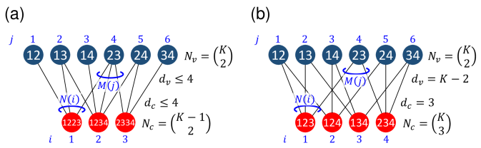
Figure 2: Two representations of bipartite graph for $K=4$ logical spins. The dark blue circle labeled $\left\{k,l\right\}$ represents the variable $x_{kl}$, while the red circles labeled $\left\{k,l,m,n\right\}$ or $\left\{k,l,m\right\}$ represent the weight-4 syndrome $s_{klmn}^{(4)}$ and weight-3 syndrome $s_{klm}^{(3)}$, respectively. In these diagrams, let us relabel the variables with blue letters. An element of code-word vector $\boldsymbol{x}=\left(x_{1},\ldots,x_{N_{v}}\right)\in\left\{+1,-1\right\}^{N_{v}}$ is called variable node (VN). The $i$-th syndrome of $\boldsymbol{x}$ is defined by $s_{i}\left(\boldsymbol{x}\right)=\prod_{k\in N\left(i\right)}x_{k}\in\left\{+1,-1\right\}$ and an element of vector $\boldsymbol{s}(\boldsymbol{x})=\left(s_{1}\left(\boldsymbol{x}\right),\ldots,s_{N_{c}}\left(\boldsymbol{x}\right)\right)\in\left\{+1,-1\right\}^{N_{c}}$ is called check node (CN), where $N\left(i\right)=\left\{j:H_{ij}(H_{ij}^{{}^{\prime}})=1\right\}$ is the VNs adjacent to a CN $i$ $\left(1\leq i\leq N_{c}\right)$ and $M\left(j\right)=\left\{i:H_{ij}(H_{ij}^{{}^{\prime}})=1\right\}$ is the CNs adjacent to a VN $j$ $\left(1\leq j\leq N_{v}\right)$. The column and row weights of the parity-check matrix are defined by $d_{v}(i)=\left|M\left(j\right)\right|$ and $d_{c}(i)=\left|N\left(i\right)\right|$, respectively.

Next, an example of a PE architecture is described. The PE architecture corresponds to the following map: $\bar{z}_{ij}=\bar{Z}_{i}\oplus\bar{Z}_{j}$ for $1\leq i\leq j\leq k$. As a simple example, consider the case $K=4$ and assume that $\boldsymbol{\bar{Z}}=\left(\bar{Z}_{1},\bar{Z}_{2},\bar{Z}_{3},\bar{Z}_{4}\right)\in\left\{0,1\right\}^{K}$ and $\bar{\boldsymbol{z}}=\left(\bar{z}_{12},\bar{z}_{13},\bar{z}_{14},\bar{z}_{23},\bar{z}_{24},\bar{z}_{34}\right)\in\left\{0,1\right\}^{\tbinom{K}{2}}$. Suppose that the generating matrix is given by $K\times\tbinom{K}{2}$ matrix:

$$\boldsymbol{G}=\begin{pmatrix}1&1&1&0&0&0\\ 1&0&0&1&1&0\\ 0&1&0&1&0&1\\ 0&0&1&0&1&1\end{pmatrix}.$$ (16)

Note that there are two 1s in each column of $\boldsymbol{G}$. This is because each element of $\bar{\boldsymbol{z}}$ is the binary sum of two elements of $\boldsymbol{\bar{Z}}$. We can consider the following two parity check matrices that is,

$$\boldsymbol{H}=\begin{pmatrix}1&1&0&1&0&0\\ 0&1&1&1&1&0\\ 0&0&0&1&1&1\end{pmatrix}$$ (17)

and

$$\boldsymbol{H}^{\prime}=\begin{pmatrix}1&1&0&1&0&0\\ 1&0&1&0&1&0\\ 0&1&1&0&0&1\\ 0&0&0&1&1&1\end{pmatrix},$$ (18)

which are sparse matrices with mostly $0$s and relatively few $1$s when $K$ is very large. It is easy to confirm that these parity check matrices satisfy the constraints $\boldsymbol{G}\boldsymbol{H}^{T}=\boldsymbol{G}\boldsymbol{H}^{\prime}{}^{T}=\boldsymbol{0}$. From these matrices, two different syndrome vectors can be derived. One is weight-4 syndrome vector $\boldsymbol{\bar{s}}^{(4)}(\bar{\boldsymbol{x}})=\left(\bar{s}_{1223}^{(4)},\bar{s}_{1234}^{(4)},\bar{s}_{2334}^{(4)}\right)=\bar{\boldsymbol{x}}\boldsymbol{H}^{T}\in\left\{0,1\right\}^{\tbinom{K-1}{2}}$, and the other is weight-3 syndrome vector $\boldsymbol{\bar{s}}^{(3)}(\bar{\boldsymbol{x}})=\left(\bar{s}_{123}^{(3)},\bar{s}_{124}^{(3)},\bar{s}_{134}^{(3)},\bar{s}_{234}^{(3)}\right)=\bar{\boldsymbol{x}}\boldsymbol{H}^{\prime}{}^{T}\in\left\{0,1\right\}^{\tbinom{K}{3}}$, where $\bar{\boldsymbol{x}}=\left(\bar{x}_{12},\bar{x}_{13},\bar{x}_{14},\bar{x}_{23},\bar{x}_{24},\bar{x}_{34}\right)\in\left\{0,1\right\}^{\tbinom{K}{2}}$ is an arbitrary binary vector. Only $2^{K}$ elements out of $2^{\tbinom{K}{2}}$ possible $\bar{\boldsymbol{x}}$ are valid code-words satisfying the parity check constraints $\boldsymbol{\bar{s}}^{(4)}(\bar{\boldsymbol{x}})=\boldsymbol{0}_{1\times\tbinom{K-1}{2}}$ or $\boldsymbol{\bar{s}}^{(3)}(\bar{\boldsymbol{x}})=\boldsymbol{0}_{1\times\tbinom{K}{3}}$. The connection between the variables $\bar{x}_{kl}$ and the weight-4 syndromes $\bar{s}_{klmn}^{(4)}$ can be represented graphically by a sparse bipartite graph shown in Fig.2(a). Similarly, the connection between variables $\bar{x}_{kl}$ and the weight-3 syndromes $\bar{s}_{klm}^{(3)}$ can be represented graphically as shown in Fig.2(b). The number of elements in $\bar{\boldsymbol{x}}$ is $N_{v}=\tbinom{K}{2}$, while the number of elements in $\boldsymbol{\bar{s}}^{(4)}(\bar{\boldsymbol{x}})$ and $\boldsymbol{\bar{s}}^{(3)}(\bar{\boldsymbol{x}})$ is $N_{c}=\tbinom{K-1}{2}$ and $N_{c}=\tbinom{K}{3}$, respectively. In the terminology of the graph theory, the $N_{v}$ elements in $\bar{\boldsymbol{x}}$ constitute variable nodes (VNs) and the $N_{c}$ elements in $\boldsymbol{\bar{s}}^{(4)}(\bar{\boldsymbol{x}})$ or $\boldsymbol{\bar{s}}^{(3)}(\bar{\boldsymbol{x}})$ constitute check nodes (CNs). The matrix $\boldsymbol{H}$ or $\boldsymbol{H}^{\prime}$ has $N_{c}$ rows and $N_{v}$ columns where each row $i$ represents a CN and each column $j$ represents a VN; If the entry $H_{ij}=1$, VN $j$ is connected to CN $i$ by edge. Thus, each edge connecting VN and CN corresponds to entry $1$ in the row and column of $\boldsymbol{H}$ or $\boldsymbol{H}^{\prime}$. Let $d_{c}$ be the number of $1$s in each row and $d_{v}$ be the number of $1$s in each column of $\boldsymbol{H}$ or $\boldsymbol{H}^{\prime}$. These numbers characterize the number of edges connected to a VN and a CN, respectively, called row and column weights. The matrix $\boldsymbol{H}^{\prime}$ is regular, and its row weight $d_{c}=3$ is common for all the CNs, and its column weight $d_{v}=K-2$ is common for all the VNs. In contrast, The matrix $\boldsymbol{H}$ is irregular, and its weights depend on the associated nodes and are at most 4. Since the weight-3 syndrome is written as a linear combination of three elements in $\bar{\boldsymbol{x}}$: $\bar{s}_{klm}^{(3)}=\bar{x}_{kl}\oplus\bar{x}_{lm}\oplus\bar{x}_{km}$, where $1\leq k<l<m\leq K$, its spin representation $s_{klm}^{(3)}$ is written as a product of three elements in $\boldsymbol{x}$: $s_{klm}^{(3)}=x_{kl}x_{lm}x_{km}$ (see Eq.(8)). Similarly, $s_{klmn}^{(4)}$ is written as a product of four elements in $\boldsymbol{x}$ if $\boldsymbol{x}$ is complemented by the fictitious spin variables $x_{ii}\,(i=2,\ldots,K-1)$ having fixed value 1: $s_{klmn}^{(4)}=x_{km}x_{lm}x_{ln}x_{kn}$ Lechner et al. (2015). It should be noted that any element in $\boldsymbol{\bar{s}}^{(4)}(\bar{\boldsymbol{x}})$ can be written as a linear combination of appropriate elements in $\boldsymbol{\bar{s}}^{(3)}(\bar{\boldsymbol{x}})$, and vice versa. Similarly, in the spin representation, any element in $\boldsymbol{s}^{(4)}(\boldsymbol{x})$ can be written as a product of appropriate elements in $\boldsymbol{s}^{(3)}(\boldsymbol{x})$, and vice versa.

$K$	$\tbinom{K}{2}$	$\tbinom{K-1}{2}$	$\tbinom{K}{3}$	$K-2$
4	6	3	4	2
5	10	6	10	3
6	15	10	20	4
7	21	15	35	5

Table 1: Parameters related to Fig.2 for $4\leq K\leq 7$.

Let us consider the graph in Fig.3, which is a graph topologically equivalent to Fig.2(a). We can see that this is nothing but the SLHZ system. It can also be seen that $H^{code}\left(\boldsymbol{z}\right)$ in Eq.(9) agrees with the Hamiltonian of the SLHZ system. Therefore, it was confirmed that there is a close connection between the SLHZ system and the word MAP decoding of the LDPC codes. Furthermore, since the two formulations for word MAP decoding, i.e. those based on $H^{code}\left(\boldsymbol{z}\right)$ (Eq.(9)) and those based on $H^{source}\left(\boldsymbol{Z}\right)$ (Eq.(5)) are mathematically equivalent, it follows that finding the ground state of the Hamiltonian of the SLHZ system is equivalent to finding the ground state of the spin glass.

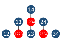
Figure 3: Bipartite graph topologically equivalent to Fig.2(a). This graph avoids any edge crossings.

III.2 Decoding readout of the SLHZ system

Bit flipping decoding algorithm

Now, let us consider decoding the readout of the SLHZ system from the perspective of the LDPC codes. To begin with, we consider the simplest case, i.e. the correction of errors caused by i.i.d. noise. This is a reasonable model for noisy communication systems as well as QA when measurement errors dominate over other sources of error in the readout. We show that a simple decoding algorithm with very low decoding complexity can be used in this case. Our decoding algorithm only uses information about the syndrome vector $\boldsymbol{s}\left(\boldsymbol{x}\right)$ to eliminate errors in the current $\boldsymbol{x}$. Furthermore, our algorithm is a symmetric decoder since all spin variables are treated symmetrically. It should be noted here that the syndrome vector depends only on the error pattern $\boldsymbol{e}=\boldsymbol{x}\boldsymbol{z}=\left(e_{12},\ldots,e_{K-1\,K}\right)\in\left\{\pm 1\right\}^{\tbinom{K}{2}}$, where multiplication is componentwise. This is because

$$\boldsymbol{s}\left(\boldsymbol{z}\right)=\left(\prod_{\left\{j:H_{1j}=1\right\}}z_{j},\ldots,\prod_{\left\{j:H_{N_{c}j}=1\right\}}z_{j}\right)=\left(+1,\ldots,+1\right)$$ (19)

holds for any code-state $\boldsymbol{z}$, and therefore

$$\boldsymbol{s}\left(\boldsymbol{x}\right)=\boldsymbol{s}\left(\boldsymbol{z}\boldsymbol{e}\right)=\boldsymbol{s}\left(\boldsymbol{z}\right)\cdot\boldsymbol{s}\left(\boldsymbol{e}\right)=\boldsymbol{s}\left(\boldsymbol{e}\right)$$ (20)

holds, where $\cdot$ denotes the inner product. Note that, in general, we only know $\boldsymbol{x}$ but never know $\boldsymbol{e}$. Since LDPC codes are linear codes, and the AWGN channel is assumed to be symmetric, i.e. $P\left(y_{i}|z_{i}\right)=P\left(-y_{i}|-z_{i}\right)$ holds, the success probability of decoding is independent of the input code-state $\boldsymbol{z}$ Richardson and Urbanke (2001).

The proposed decoding algorithm corresponds to a sort of Gallager’s BF decoding algorithm in the spin representation Gallager (1962, 1963). It is based on Massey’s APP (a posteriori probability) threshold decoding algorithm Massey (1962). Not the weight-4 but the weight-3 syndrome $s_{ijk}^{(3)}\left(\boldsymbol{x}\right)=x_{ij}x_{jk}x_{ik}=e_{ij}e_{jk}e_{ik}$ is used to decode the current decision $\boldsymbol{x}$ because it has the advantage of treating all variables (VN and CN) symmetrically Pastawski and Preskill (2016). The trade-off is that more constraints may increase the decoding complexity. However, as will be shown later, this is not the case for us since symmetry can be used to reduce computational costs. To obtain the best estimate $e_{ij}^{*}\in\left\{\pm 1\right\}$ of error $e_{ij}$, we use the syndromes $s_{ijk}^{(3)}\left(\boldsymbol{x}\right)$ with $k\neq i,j$, which are considered an $K-2$ parity checks orthogonal on $e_{ij}$ Massey (1962). The value of the syndrome $s_{ijk}^{(3)}\left(\boldsymbol{x}\right)$ indicates whether the parity-check equation is satisfied (being $+1$) or violated (being $-1$). Based on this value, we decide a spin to be flipped or not. There are $N_{v}=\tbinom{K}{2}$ choices for the set $\left\{i,j\right\}$, and the associated syndromes $s_{ijk}^{(3)}\left(\boldsymbol{x}\right)$’s are computed from a hard decision $\boldsymbol{x}$ of the observation $\boldsymbol{y}$. The estimate $e_{ij}^{*}$ is obtained from the APP decoding by weighted majority voting Massey (1962)

$$e_{ij}^{*}=\mathrm{sign}\left(w_{0}+\sum_{k\neq i,j}^{K}w_{k}s_{ijk}^{(3)}\left(\boldsymbol{x}\right)\right)=\mathrm{sign}\left[\varDelta_{ij}\left(\boldsymbol{x}\right)\right],$$ (21)

where $w_{0}>0$ is the weighting factor associated with the reliability $\left|\theta_{ij}\right|$ of the hard decision $x_{ij}=\mathrm{sgn}\left[y_{ij}\right]$:

$$w_{0}=\left|\theta_{ij}\right|=\log\frac{1-\gamma_{ij}}{\gamma_{ij}}.$$ (22)

Here, $w_{0}=\beta\left|y_{ij}\right|$ for the AWGN channel and $\gamma_{ij}$ is an error probability that $x_{ij}$ is in error

$$\gamma_{ij}=P\left(x_{ij}=-z_{ij}\right)=P\left(e_{ij}=-1\right).$$ (23)

The positive parameter $w_{k}$ is a weighting factor associated with the reliability of the $k$th parity check for the decision of $e_{ij}$:

$$w_{k}=\log\frac{1-p_{k}}{p_{k}},$$ (24)

where $p_{k}$ is a probability that a decision based on $s_{ijk}^{(3)}$ is in error:

$$p_{k}=P\left(s_{ijk}^{(3)}=-e_{ij}\right)=P\left(e_{jk}e_{ik}=-1\right).$$ (25)

In Eq.(21), $e_{ij}^{*}=-1$ means that the sign of $x_{ij}$ should be flipped so that $x_{ij}\rightarrow x_{ij}e_{ij}=-x_{ij}$. Function $\varDelta_{ij}\left(\boldsymbol{x}\right)$ is called the inversion function and determines whether the spin variable $x_{ij}$ should be flip its sign ($e_{ij}^{*}=-1$) or not ($e_{ij}^{*}=1$) Wadayama et al. (2010); Sundararajan et al. (2014). Parameters $\gamma_{ij}$ and $p_{k}$ are considered to be those parameters that characterize the binary symmetric channels shown in Fig.4. We should note that the probability $p_{k}$ is given by the probability of an odd number of $-1$s among the errors exclusive of $e_{ij}$ that are checked by $s_{ijk}^{(3)}\left(\boldsymbol{x}\right)=e_{ij}e_{jk}e_{ik}$ so that it is given by Massey (1962)

$$p_{k}=P\left(e_{jk}e_{ik}=-1\right)=\frac{1}{2}\left(1-\left(1-2\gamma_{jk}\right)\left(1-2\gamma_{ik}\right)\right).$$ (26)

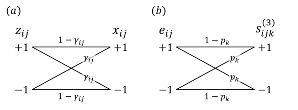
Figure 4: Binary symmetric channel associated with the parameters $\gamma_{ij}$ and $p_{k}$.

Since we assumed i.i.d. noise, $\gamma_{ij}=\gamma_{0}$ holds for every $\left\{i,j\right\}$ for which $\gamma_{0}$ is a constant. In this case, assuming $1\leq\gamma_{0}<\tfrac{1}{2}$, we can confirm that $w_{0}$ can be approximated as $w_{0}=w_{k}$ for any $k$. Thus, we obtain the following algorithm: we calculate the best estimate by

$$e_{ij}^{*}=\mathrm{sign}\left(1+\sum_{k\neq i,j}^{K}s_{ijk}^{(3)}\left(\boldsymbol{x}\right)\right).$$ (27)

This equation means that if the majority vote of $\left\{1,s_{ij1}^{(3)}\left(\boldsymbol{x}\right),\ldots,s_{ijK}^{(3)}\left(\boldsymbol{x}\right)\right\}\in\left\{\pm 1\right\}^{K+1}$ is negative, $x_{ij}$ should be flipped to increase the value of $\sum_{k\neq i,j}^{K}s_{ijk}^{(3)}\left(\boldsymbol{x}\right)$. Thus, Eq.(27) is reduced to the following equation for the best estimate $z_{ij}\in\left\{\pm 1\right\}$:

$$z_{ij}=x_{ij}e_{ij}^{*}=\mathrm{sign}\left(x_{ij}+\sum_{k\neq i,j}^{K}x_{jk}x_{ki}\right),$$ (28)

where we used the fact $x_{ij}\in\left\{\pm 1\right\}$. This expression is represented only in terms of the values of VNs. Eq.(27) can be interpreted as the Gallager’s BF decoding Gallager (1962, 1963). Fig.5 shows the relevant bipartite graph for $K=5$. Note that the graph associated with the SLHZ system is more loopy, with a minimum length of 4, whereas this graph is less loopy, with a minimum length of 6. The initial decision $\boldsymbol{x}$ on the VNs, hard-decided by $\boldsymbol{y}$, is broadcasted to its adjacent CNs connected by edges. Each CN then reports the syndrome value to its adjacent VNs connected by the edge. All VNs update their values simultaneously according to Eq.(27), representing a majority vote of 1 and the associated value of adjacent CNs.

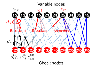
Figure 5: Bipartite graph for $K=5$ logical spins. Solid blue lines show an example of the shortest loop of edges connecting VNs and CNs, which has a length of 6.

Application to the SLHZ system

This subsection describes how our decoding applies to the SLHZ system. Consider a matrix representation of the state of the SLHZ system. Let us introduce the $K\times K$ symmetrized matrix $\hat{\boldsymbol{z}}$ whose entries are given by spin variable $z_{ij}=z_{ji}\in\left\{\pm 1\right\}$ and having unit diagonal elements, namely,

$$\hat{\boldsymbol{z}} = \left[\begin{array}[]{cccccc}1&z_{12}&z_{13}&\cdots&z_{1\,K-1}&z_{1\,K}\\ z_{21}&1&z_{23}&\cdots&z_{2\,K-1}&z_{2\,K}\\ z_{31}&z_{32}&1&\cdots&z_{3\,K-1}&z_{3\,K}\\ \vdots&\vdots&\vdots&\ddots&\cdots&\vdots\\ z_{K-1\,1}&z_{K-1\,2}&z_{K-1\,3}&\cdots&1&z_{K-1\,K}\\ z_{K\,1}&z_{K\,2}&z_{K\,3}&\cdots&z_{K\,K-1}&1\end{array}\right]$$ (35)

$$\in \left\{\pm 1\right\}^{K\times K}.$$ (36)

We use similar notations $\hat{\boldsymbol{x}}$ and $\hat{\boldsymbol{e}}$ for the symmetrized matrices associated with current $\boldsymbol{x}$ and error pattern $\boldsymbol{e}$. They satisfy $\hat{\boldsymbol{x}}=\hat{\boldsymbol{z}}\circ\hat{\boldsymbol{e}}$, where $\circ$ denotes componentwise multiplication. Hereafter, we will call $\hat{\boldsymbol{e}}$ the error matrix. Then, Eq.(28) can be conveniently written as

$$\hat{\boldsymbol{z}}=\mathcal{F}\left(\hat{\boldsymbol{x}}\right)=\mathrm{sign}\left[\hat{\boldsymbol{x}}\left(\hat{\boldsymbol{x}}-\boldsymbol{I}_{K\times K}\right)\right],$$ (37)

where the sign function is componentwise. This operation updates the $\tbinom{K}{2}$ elements in $\hat{\boldsymbol{x}}$ in parallel. Therefore, Eq.(37) represents a parallel BF algorithm. We further consider iterative operation of $\mathcal{F}$, i.e.,

$$\hat{\boldsymbol{z}}^{(n)}=\hat{\boldsymbol{z}}\circ\hat{\boldsymbol{e}}^{(n)}=\mathcal{F}^{(n)}\left(\hat{\boldsymbol{x}}\right).$$ (38)

If $\hat{\boldsymbol{z}}^{(n)}\rightarrow\hat{\boldsymbol{z}}$, or in other words $\hat{\boldsymbol{e}}^{(n)}\rightarrow\boldsymbol{I}_{K\times K}$, at $n=n_{0}$, we say that the decoding was succeeded after $n_{0}$ iteration of the BF decoding. In the case of success, it follows that $s_{ijk}^{(3)}\left(\hat{\boldsymbol{z}}\right)=1$ for a set of possible $\left\{i,j,k\right\}$ at $n=n_{0}$. Our algorithm can safely be stated as an iterative process that gradually increases the syndrome values by flipping spins according to the majority vote of an associated set of relevant syndrome values.

IV Experimental demonstration

We demonstrate the validity and performance of the BF algorithm and compare it to those of standard BP algorithm and the word MAP decoding using the Monte Carlo sampling. In addition, the results are shown when the BF decoding is applied to a stochastically sampled readout of the SLHZ system.

IV.1 I.i.d. noise model

First, the performance of the BF algorithm was investigated assuming i.i.d noise, a simple model of the noisy readout of the SLHZ system. PP previously studied this model with the BP algorithm Pastawski and Preskill (2016). Note that the BF decoding in Eq.(27) depends only on the weight-3 syndromes, which treat all variables (VN and CN) symmetrically Pastawski and Preskill (2016). In this case, without loss of generality, the performance of decoding can be analyzed using the assumption that all-one code-state $\boldsymbol{z}=\left(+1,\ldots,+1\right)$ has been transmitted Richardson and Urbanke (2001); Vuffray (2014). In physics, this assumption corresponds to choosing the ferromagnetic gauge and representing the current decision $\boldsymbol{x}$ by an error pattern $\boldsymbol{e}$. We assume the input is all-one code-state, that is, $\hat{\boldsymbol{z}}=\hat{\boldsymbol{1}}_{K\times K}$, where $\hat{\boldsymbol{1}}_{K\times K}$ is $K\times K$ matrix whose entries are all one (all-one matrix). All the demonstration was performed using the Mathematica^® Ver.14 platform on the Windows 11 operating system. We generated 5000 symmetric matrices $\hat{\boldsymbol{x}}=\hat{\boldsymbol{e}}$ with unit diagonal elements and other elements randomly assigned to $-1$ with probability $\varepsilon<\tfrac{1}{2}$ and $+1$ otherwise. After $n=5$ iterations, the BF decoding was checked to see if the error was removed. Figure 6(a) shows the performance of the BF algorithm, plotting the probability of decoding failure as a function of the number $K$ of logical spins for $K$ ranging from $2$ to $40$ and seven values of $\varepsilon$ $\left(=0.05,0.07,0.1,0.15,0.2,0.3,0.4\right)$. Note that the associated SLHZ model consists of $\tbinom{K}{2}$ physical spins. The failure probability falls steeply as $N$ increases if $\varepsilon$ is not too close to the threshold value $1/2$. A similar performance calculation was reproduced for the decoding based on the BP algorithm given by PP, assuming that it is iterated five times, as shown in Fig.6(b) Pastawski and Preskill (2016). Comparing these figures, we can see that the performance of the BF algorithm is comparable to that of the BP algorithm. Note that in the BP algorithm, all marginal probability $P\left(x_{i}|\boldsymbol{y}\right)$ associated with the $\tbinom{K}{2}$ spins are updated sequentially by passing a real-valued message between the associated VNs and CNs in a single iteration. In contrast, in the BF algorithm, all the $\tbinom{K}{2}$ variables $x_{ij}$ in the matrix $\hat{\boldsymbol{x}}$ are updated in parallel in a single iteration. Thus, in these performance evaluations, each variable was updated the same number of times, i.e., five times, in both the BF and BP algorithms.

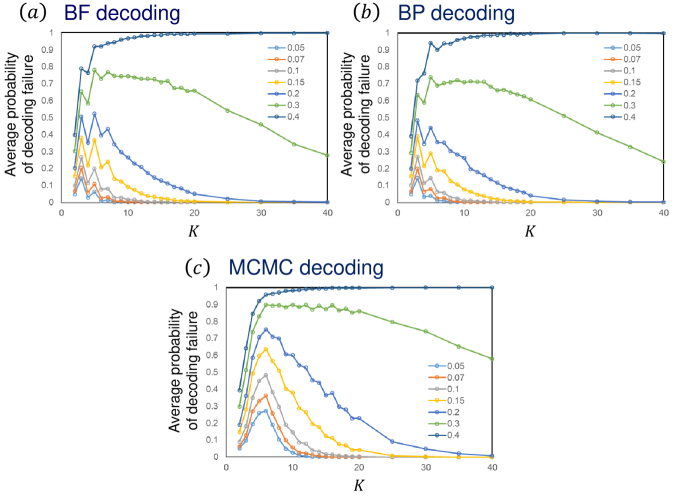
Figure 6: Comparison of performance of (a) BF, (b) BP and (c) MCMC decodings. Assuming that the error probability $\varepsilon$ is common to all physical spins, the average probabilities of decoding failure is plotted as a function of the number $K$ of logical spins (associated with $\tbinom{K}{2}$ physical spins) for seven values of $\varepsilon$. Each data point was obtained by averaging over 5000 error matrix realizations. For each realization, the BF and BP algorithms were iterated five times, and the MCMC sampling was iterated $\tbinom{K}{2}$ times. We considered a tie in the majority voting as a failure in the BF decoding, although we can resolve a tie by introducing a tie-break rule such as coin tossing.

Fig.7 is an example of a successfully decoded result when $K=40$ and $\varepsilon=0.3$. In this figure, each entry of the error matrix $\hat{\boldsymbol{e}}$ is plotted after $n=1,\ldots,4$ iterations of the operation in Eq.(37). The blue pixels correspond to spins with error, the number of which gradually decreases as rounds of iteration are added. In this example, an error-free matrix was obtained after $n=3$ iterations. Such results were observed for more than $70$ % of the error matrices generated.

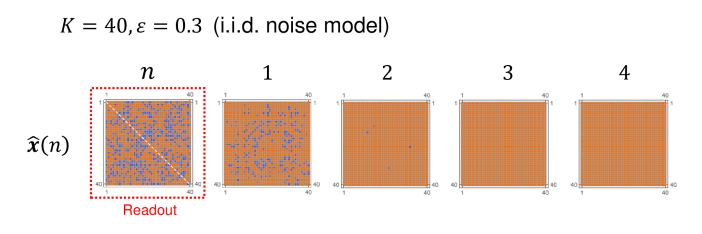
Figure 7: An example of successfully decoded results by the BF decoding when $K=40$ and $\varepsilon=0.3$. The initial readout was generated in accordance with the i.i.d. noise model. The estimated matrix $\hat{\boldsymbol{x}}$ is plotted from left to right in increasing order of iterations $n$. The blue pixels represent spins with error.

In addition to the BF and BP algorithms, let us focus on the word MAP decoding introduced in II.2 of the section II and compare its performance with the above algorithms. The word MAP decoding says that the code-state is the ground state of the Hamiltonian, as shown in Eq.(9), that is,

$$H^{code}\left(\hat{\boldsymbol{x}}\right)\equiv\gamma\sum_{\left\{i,j,k\right\}}\frac{1-s_{ijk}^{(3)}\left(\hat{\boldsymbol{x}}\right)}{2},$$ (39)

where $\hat{\boldsymbol{x}}\in\left\{\pm 1\right\}^{K\times K}$ is the matrix representing the general state of the SLHZ system. In general, $H^{code}\left(\hat{\boldsymbol{x}}\right)\geq 0$ and $H^{code}\left(\hat{\boldsymbol{x}}\right)=0$ if and only if $\hat{\boldsymbol{x}}$ is a code-state. In Eq.(39), the correlation term (the first term in Eq.(9)) was omitted. This is because the all-one code-state assumption uses no information about the observation $\boldsymbol{y}$. Under this assumption, the ground state of $H^{code}\left(\hat{\boldsymbol{x}}\right)$ is given by

$$\hat{\boldsymbol{z}}=\underset{\hat{\boldsymbol{x}}\in\left\{\pm 1\right\}^{K\times K}}{\arg\min}H^{code}\left(\hat{\boldsymbol{x}}\right)=\hat{\boldsymbol{1}}_{K\times K}.$$ (40)

The performance of word MAP decoding was evaluated based on the Hamiltonian $H^{code}\left(\hat{\boldsymbol{x}}\right)$ given by Eq.(39). We generated 5000 random symmetric matrices $\hat{\boldsymbol{e}}$ whose entries are $-1$ with probability $p<\frac{1}{2}$ and $+1$ otherwise. The classical MCMC sampler was used to search for the ground state of $H^{code}\left(\hat{\boldsymbol{x}}\right)$ from the initial state $\hat{\boldsymbol{x}}=\hat{\boldsymbol{e}}$. Hyperparameter $\gamma$ was assigned to $\gamma\approx 1$, which was experimentally optimal. We examined to see if the ground state $\hat{\boldsymbol{z}}$ could be found in a set of estimate $\left\{\hat{\boldsymbol{x}}\right\}$ sampled by MCMC. In this sampling, we used rejection-free MCMC sampling, in which all self-loop transitions are removed from the standard MCMC Nambu (2022) and the size of $\left\{\hat{\boldsymbol{x}}\right\}$ was restricted to $\tbinom{K}{2}$. Figure 6(c) indicates the performance of the word MAP decoding using the MCMC sampler, which we called the MCMC decoding. Although its performance is not as good as that of the BF and BP algorithms, it shows a similar dependence on $K$ and $\varepsilon$. This result is quite reasonable as well as suggestive. Later, we will discuss the reason.

IV.2 Beyond the i.i.d. noise model

As the development of QA devices is ongoing and classical simulation of a quantum-mechanical many-body system is computationally challenging, it is difficult to verify whether our BF decoding algorithm provides good protection against noise in physical spin readouts of QA, not only by classical computer simulations but also by an actual QA device. Instead, we tested the potential of our BF decoding algorithm by simulating the hard-decided readout of spins in the SLHZ system with stochastically sampled data by a classical MCMC sampler.

We used the following Hamiltonian to obtain stochastically sampled data for the SLHZ system:

$$H^{code}\left(\hat{\boldsymbol{x}}\right)\equiv-\beta\sum_{\left\{i,j\right\}}J_{ij}x_{ij}+\gamma\sum_{\left\{i,j,k,l\right\}}\frac{1-s_{ijkl}^{(4)}\left(\hat{\boldsymbol{x}}\right)}{2},$$ (41)

where $J_{ij}\in\mathbb{R}^{\tbinom{K}{2}}$ is a coupling constant identified with the channel observation $y_{ij}\in\mathbb{R}^{\tbinom{K}{2}}$ in the AWGN channel model. Parameters $\left\{\beta,\gamma\right\}$ are independent annealing parameters to be adjusted. If the weight-4 syndrome is defined by

$$s_{ijkl}^{(4)}\left(\hat{\boldsymbol{x}}\right)=x_{ik}x_{jk}x_{jl}x_{il},$$ (42)

with assumption $x_{ii}=1$ for $i=1,\ldots,K$, Eq.(41) is just the Hamiltonian of the SLHZ system given in Fig.3. The $\left(K-1\right)$-degenerated ground state of the second term in Eq.(41) defines the code-states. Sampling from low-temperature equilibrium state $\hat{\boldsymbol{x}}$ of $H^{code}\left(\hat{\boldsymbol{x}}\right)$, we can see which is most likely to be the code-state given by matrix $\hat{\boldsymbol{z}}=\boldsymbol{Z}^{T}\boldsymbol{Z}$ that minimizes $H^{code}\left(\hat{\boldsymbol{x}}\right)$, as shown in Eq.(40), where $\boldsymbol{Z}=\left(Z_{1},\ldots,Z_{K}\right)\in\left\{\pm 1\right\}^{K}$ is the source-state. This is nothing but the word MAP decoding. However, in this case, $\hat{\boldsymbol{z}}=\hat{\boldsymbol{1}}_{K\times K}$ cannot be assumed in the evaluation of performance, in contrast to Eq.(40). This is because both the correlation term (first term) as well as the penalty term (second term) in Eq.(41) violate the symmetry conditions required for all-one code-state assumption to hold in this case. As a result, the performance of the word MAP decoding based on Eq.(41) depends not only on the error distribution $\hat{\boldsymbol{e}}$ but also on $\hat{\boldsymbol{z}}$ .

Our BF algorithm is also valid for the readout of the SLHZ system sampled by a classical MCMC sampler. We show an illustrative example to see this. We simulated readouts $\hat{\boldsymbol{x}}\in\left\{\pm 1\right\}^{K\times K}$ of the SLHZ system associated with a spin glass problem for $K=14$ as a toy model using the MCMC sampler, where the code-state $\hat{\boldsymbol{z}}$ for a given $\boldsymbol{J}=\left(J_{12},\ldots,J_{K-1\,K}\right)\in\left\{\pm 1\right\}^{\tbinom{K}{2}}$ was precomputed by brute force. The leftmost matrix plot in Fig.8 visualizes an example of the error matrix $\hat{\boldsymbol{e}}=\hat{\boldsymbol{x}}\circ\hat{\boldsymbol{z}}$ associated with a sampled readout $\hat{\boldsymbol{x}}$ of the SLHZ system. In this example, the error distribution was different from the expected when assuming an i.i.d. noise model, as shown in Fig.7. This suggests that our BF algorithm, as well as the BP algorithm, can correct errors in the stochastically sampled readouts of the SLHZ system.

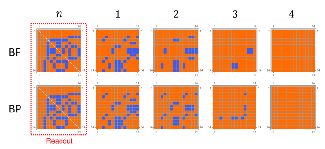
Figure 8: Examples of successful BF and BP decoding for $K=14$ logical spins. An MCMC sampler sampled readout based on the Hamiltonian $H^{code}\left(\hat{\boldsymbol{x}}\right)$ of Eq.(41). See details in the main text. The readout matrix $\hat{\boldsymbol{x}}$ is plotted from left to right in order of increasing number of iterations $n$ of two algorithms. The blue pixels represent spins with error.

The MCMC sampling was performed as follows. We sampled a sequence $\left\{\hat{\boldsymbol{x}}\right\}$ of estimated states using a rejection-free MCMC sampler starting from a random state. After a certain number of MCMC samplings, we checked whether $\left\{\hat{\boldsymbol{x}}\right\}$ involves $\hat{\boldsymbol{z}}$ or not. If $\left\{\hat{\boldsymbol{x}}\right\}$ involves $\hat{\boldsymbol{z}}$, the sequence was successfully decoded. Otherwise, it fails. The performance can be evaluated by repeating the same experiment independently, obtaining many sampled sequences $\left\{\hat{\boldsymbol{x}}\right\}$, and measuring the average probability of succeeded sequences.

We call a search of the ground state of $H^{code}\left(\hat{\boldsymbol{x}}\right)$, which is equivalent to the word MAP decoding, using the MCMC sampler the MCMC decoding as stated before. In addition, we also performed two-stage hybrid decoding. In this strategy, the sequence $\left\{\hat{\boldsymbol{x}}\right\}$ is sampled by the MCMC sampler in the first stage. Each element of the sequence $\left\{\hat{\boldsymbol{x}}\right\}$ is then decoded using the BF decoding in the second stage to correct the errors in each $\hat{\boldsymbol{x}}$ and updated to $\left\{\hat{\boldsymbol{w}}\right\}$. Then, if $\left\{\hat{\boldsymbol{w}}\right\}$ involves $\hat{\boldsymbol{z}}$, the sequence was successfully decoded, otherwise it failed. We call this strategy the MCMC-BF hybrid decoding. We can evaluate its performance as well. The MCMC decoding can be identified with simulated annealing. Similarly, the MCMC-BF hybrid decoding can be identified with simulated annealing and subsequent classical error correction.

The performance of these decoding strategies depends not only on the annealing parameters $\left\{\beta,\gamma\right\}$ but also on the strategy as shown in Fig.9. The columns (a) and (b) indicate landscapes of the success probability for (a) the MCMC decoding and (b) the MCMC-BF hybrid decoding, respectively. In these figures, the top two figures are the probability of success in finding the correct code-state $\hat{\boldsymbol{z}}=\boldsymbol{Z}^{T}\boldsymbol{Z}$, and the bottom two figures are the probability of finding any code-state $\hat{\boldsymbol{x}}=\boldsymbol{X}^{T}\boldsymbol{X}$, where $\boldsymbol{X}\in\left\{\pm 1\right\}^{K}$ is any logical state. It is very important to note that the size of the sample $\left\{\hat{\boldsymbol{x}}\right\}$ differs significantly between the two decoding strategies; it was $1200\tbinom{K}{2}$ for the MCMC decoding and $4\tbinom{K}{2}$ for the MCMC-BF hybrid decoding, which were determined by the number of iterations of the rejection-free MCMC loops. The readers can understand that the MCMC-BF hybrid decoding provides a better trade-off between error performance and decoding complexity, assuming that the decoding complexity of the BF decoding is negligible. We will revisit the validity of this assumption later.

Let us note that two arrows $A$ and $B$ in Fig.9. These arrows indicate two annealing parameter sets $A=\left\{\beta_{A},\gamma_{A}\right\}$ and $B=\left\{\beta_{B},\gamma_{B}\right\}$. The set $A$ corresponds to parameters for which the MCMC decoding is highly efficient, and the set $B$ corresponds to the parameters for which the MCMC-BF hybrid decoding is highly efficient. The left and right plots in Fig. 10 are the matrix plots showing average error matrix $\left\langle\hat{\boldsymbol{e}}\right\rangle=\left\langle\hat{\boldsymbol{x}}\right\rangle\circ\hat{\boldsymbol{z}}$ over the set of samples $\left\{\hat{\boldsymbol{x}}\right\}$ of the MCMC sampler when $\left\{\hat{\boldsymbol{x}}\right\}$ was sampled with the parameter sets $A$ and $B$, respectively. A positive (negative) entry in $\left\langle\hat{\boldsymbol{e}}\right\rangle$ indicates that there is likely no error (error) in the corresponding entry in $\hat{\boldsymbol{x}}$. Thus, each entry in $\left\langle\hat{\boldsymbol{e}}\right\rangle$ reflects a marginal error probability for inferring the correct sign for that entry. We can see that they depend on the annealing parameters. The average error matrix $\left\langle\hat{\boldsymbol{e}}\right\rangle$ in Fig.10(b) is consistent with the error matrix $\hat{\boldsymbol{e}}$ in Fig.8. In fact, the error matrix $\hat{\boldsymbol{e}}$ shown in Fig.8 was an element of $\left\{\hat{\boldsymbol{x}}\right\}$ that was sampled by the MCMC sampling with the parameter set $B$. Note that the parameter set $B$ allowed little sampling for the code-state by the MCMC sampler in the first stage (see the lower left plot in Fig.9). This means that the state $\hat{\boldsymbol{x}}$ the MCMC sampler sampled in the first stage of the MCMC-BF decoding is not a code-state. This is quite reasonable because the subsequent BF decoding can correct errors in the state $\hat{\boldsymbol{x}}$ only if it is not a code-state. It is important to note that this is a feature of our BF decoding algorithm and is independent of the decoding algorithm in the first stage. Therefore, optimal annealing parameters $\left\{\beta_{opt},\gamma_{opt}\right\}$ should be different for single-stage and two-stage hybrid decoding. This suggests that optimal annealing parameters should be carefully studied when applying our BF decoding for readouts of QA; they might differ from the optimal parameters for QA when used alone.

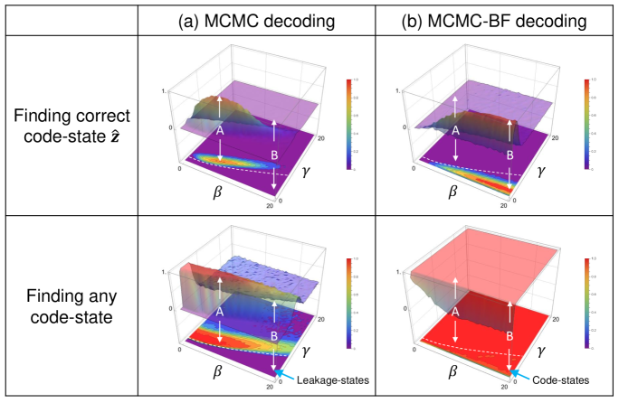
Figure 9: Landscapes of the probability distribution for successful decoding. They are plotted as functions of the annealing parameters $\left\{\beta,\gamma\right\}$. The left and right columns are the results of (a) MCMC decoding and (b) MCMC-BF hybrid decoding, respectively. On the other hand, the states searched in the upper and lower rows are different: they are the correct target state $\hat{\boldsymbol{z}}$ for the upper row and any code-states for the lower row.

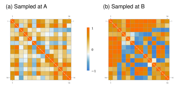
Figure 10: Matrix plots representing the averaged error matrix $\left\langle\hat{\boldsymbol{e}}\right\rangle=\left\langle\hat{\boldsymbol{x}}\right\rangle\circ\hat{\boldsymbol{z}}$ after the MCMC sampling (but before the BF decoding), where each entry reflects the marginal error probability in inferring the correct sign of the associated entry. Warm (cold) colored pixels indicate that there is likely no error (error) in the inference of the corresponding spin. The left and right plots correspond to $\left\langle\hat{\boldsymbol{e}}\right\rangle$ when $\left\{\hat{\boldsymbol{x}}\right\}$ is sampled with the parameter sets $A$ and $B$ in Fig.9, respectively.

V Discussions

V.1 Relationship between MCMC-BF hybrid algorithm and other known BF algorithms

The MCMC-BF decoding algorithm includes MCMC decoding as a preprocessing step for the BF decoding algorithm. Both the MCMC and BF decoding algorithms are hard-decision algorithms. We consider the mutual relationship between these algorithms and similar existing hard-decision algorithms.

Introducing the MCMC decoding as a preprocessing step solves two shortcomings of the postprocessing BF decoding algorithm. The first one is that the BF algorithm neglects the soft information in the observation $\boldsymbol{y}$. As mentioned, the BF algorithm assumes a symmetric channel and treats all the spin variables (VNs) and syndromes (CNs) symmetrically, justifying the all-one code-state assumption. This results from neglecting the $\boldsymbol{y}$-dependent correlation term in the Hamiltonian $H^{code}\left(\hat{\boldsymbol{x}}\right)$ in Eq.(9) (see also Eq.(39)), which breaks the required symmetry. To incorporate information involved in the correlation term, soft information in the observation $\boldsymbol{y}$ must be considered in the BF decoding. This is usually accomplished by incorporating the reliability information in the channel LLR $\theta\left(y_{i}\right)$ into the BF algorithm. The BF algorithm approximates the weighted majority formula (21) to the majority formula (27) by assuming that $\gamma_{ij}=\gamma_{0}$ for every channel decision $x_{ij}$, so soft information is lost. Although this approximation is reasonable for the i.i.d. noise model since the reliability is the same for every channel, it fails if the noise does not follow this model. In general, $\gamma_{ij}$ depends on channel index $\left\{i,j\right\}$. In the AWGN channel model, if the absolute value of channel observation $\left|y_{ij}\right|$ is small (large), hard decision $x_{ij}=\mathrm{sgn}\left[y_{ij}\right]$ is less (more) reliable. Please see Eqs.(12) and (13). It follows that the weight $\gamma_{ij}$ is small (large) if $\left|y_{ij}\right|$ is small (large). Many researchers have developed sophisticated versions of the weighted BF (WBF). See details in Refs.Khoa Le Trung (2017); Kennedy Masunda (2017) and references therein. Alternatively, there is another approach to incorporate soft information. For example, Wadayama et al. proposed the Gradient Descent Bit Flipping (GDBF) algorithm Wadayama et al. (2010). They are based on modifications to the inversion function, which may improve the decoding performance at the cost of increasing decoding complexity. For example, the inversion functions for the BF, WBF, and GDBF are formally written as

$$\varDelta_{k}^{\left(BF\right)}\left(\boldsymbol{x}\right)=1+\sum_{i\in M\left(k\right)}s_{i}\left(\boldsymbol{x}\right),$$ (43)

$$\varDelta_{k}^{\left(WBF\right)}\left(\boldsymbol{x}\right)=\beta\left|J_{k}\right|+\sum_{i\in M\left(k\right)}w_{k}s_{i}\left(\boldsymbol{x}\right),$$ (44)

and

$$\varDelta_{k}^{\left(GDBF\right)}\left(\boldsymbol{x}\right)=J_{k}x_{k}+\sum_{i\in M\left(k\right)}s_{i}\left(\boldsymbol{x}\right),$$ (45)

respectively. Here, $\boldsymbol{x}=\left(x_{1},\ldots,x_{N_{v}}\right)\in\left\{\pm 1\right\}^{N_{v}}$ is current decision (VNs) and

$$s_{i}\left(\boldsymbol{x}\right)=\prod_{j\in N\left(i\right)}x_{j}\in\left\{\pm 1\right\}$$ (46)

is $i$th syndrome (CN) for the decision $\boldsymbol{x}$ in the spin representation, $J_{k}$ is identified with channel observation $y_{k}$ in the AWGN channel model, and $\beta$ is a positive real parameter to be adjusted. Here, the set $N\left(i\right)=\left\{j:H_{ij}=1\right\}$ is the VNs adjacent to an $i$th CN $\left(1\leq i\leq N_{c}\right)$ and the set $M\left(j\right)=\left\{i:H_{ij}=1\right\}$ is the CNs adjacent to a $j$th VN $\left(1\leq j\leq N_{v}\right)$. Please refer to Fig.2 for the definition of these sets. Note that as long as $s_{i}\left(\boldsymbol{x}\right)$ is a weight-3 syndrome, $\varDelta_{k}^{\left(BF\right)}\left(\boldsymbol{x}\right)$ is symmetric for the permutation of the elements of $\boldsymbol{x}$. In other words, exchanging as $i\longleftrightarrow j$ for any pair of indices of VN other than $k$ does not change $\varDelta_{k}^{\left(BF\right)}\left(\boldsymbol{x}\right)$. In contrast, weight-4 syndrome is not symmetric. Similarly, $\varDelta_{k}^{\left(WBF\right)}\left(\boldsymbol{x}\right)$ and $\varDelta_{k}^{\left(GDBF\right)}\left(\boldsymbol{x}\right)$ are not symmetric even if $s_{i}\left(\boldsymbol{x}\right)$ is weight-3 syndrome because $\varDelta_{k}^{\left(WBF\right)}\left(\boldsymbol{x}\right)$ involves weight $w_{k}$ in the second term and $\varDelta_{k}^{\left(GDBF\right)}\left(\boldsymbol{x}\right)$ involves $J_{k}$ in the first term, both of which depends on observation $\boldsymbol{y}$.

It is interesting to note that the inversion functions in Eq.(43)-(45) can be derived from the following Hamiltonians:

$$H^{(BF)}\left(\boldsymbol{x}\right)=-\sum_{i=1}^{N_{v}}x_{i}-\sum_{i=1}^{N_{c}}s_{i}\left(\boldsymbol{x}\right),$$ (47)

$$H^{(WBF)}\left(\boldsymbol{x}\right)=-\beta\sum_{i=1}^{N_{v}}\left|J_{i}\right|x_{i}-\sum_{i=1}^{N_{c}}w_{i}s_{i}\left(\boldsymbol{x}\right),$$ (48)

$$H^{(GDBF)}\left(\boldsymbol{x}\right)=-\frac{1}{2}\sum_{i=1}^{N_{v}}J_{i}x_{i}-\sum_{i=1}^{N_{c}}s_{i}\left(\boldsymbol{x}\right).$$ (49)

If we note that when we flip the sign of $x_{k}$, that is, $x_{k}\rightarrow-x_{k}$, the increase in energy $\Delta H_{k}^{(X)}\left(\boldsymbol{x}\right)$ is given by

$$\Delta H_{k}^{(X)}\left(\boldsymbol{x}\right)=2\varDelta_{k}^{\left(X\right)}\left(\boldsymbol{x}\right),$$ (50)

where $X=BF$, $WBF$, or $GDBF$. It follows that if $\varDelta_{k}^{\left(X\right)}\left(\boldsymbol{x}\right)<0$, flipping the sign of the $k$th spin reduces the energy of the spin system. Therefore, the BF, WBF, and GDBF decoding algorithms can be considered deterministic algorithms that determine the most suitable spins to be flipped to reduce the energy $H_{k}^{(X)}\left(\boldsymbol{x}\right)$ based on the inverse function $\varDelta_{k}^{\left(X\right)}\left(\boldsymbol{x}\right)$. It should be noted that the BP algorithm, in contrast to the BF algorithm, essentially considers soft information since it is based on calculating a consistent marginal probability $P\left(x_{i}|\boldsymbol{y}\right)$ by exchanging real-valued messages between the VNs and CNs. On the other hand, the inversion function and the associated Hamiltonian for the MCMC decoding are formally written by

$$\varDelta_{k}^{\left(MCMC\right)}\left(\boldsymbol{x}\right)=\beta J_{k}x_{k}+\frac{\gamma}{2}\sum_{i\in M\left(k\right)}s_{i}\left(\boldsymbol{x}\right)$$ (51)

and

$$H^{(MCMC)}\left(\boldsymbol{x}\right)=-\beta\sum_{i=1}^{N_{v}}J_{i}x_{i}+\gamma\sum_{i=1}^{N_{c}}\frac{1-s_{i}\left(\boldsymbol{x}\right)}{2}.$$ (52)

The MCMC decoding algorithm uses MCMC sampling to find $\boldsymbol{x}$ that reduces the energy $H^{(MCMC)}\left(\boldsymbol{x}\right)$ based on the inversion function $\varDelta_{k}^{\left(MCMC\right)}\left(\boldsymbol{x}\right)$. Therefore, the MCMC decoding at the first stage intrinsically includes the soft information in $J_{k}$ in the correlation term, which resolves one shortcoming of the BF decoding.

Furthermore, introducing MCMC decoding in the first stage also solves another shortcoming. The MCMC sampling is stochastic in nature in contrast to our deterministic BF algorithm as well as gradient descent algorithm used in the GDBF algorithm. This stochastic nature introduces randomness into the spin-flip selection and allows spins to be flipped even when $\varDelta_{k}^{\left(MCMC\right)}\left(\boldsymbol{x}\right)>0$. This provides an escape from spurious local minima and is more likely to arrive at the neighborhood of the global minimum of $H^{(MCMC)}\left(\boldsymbol{x}\right)$. Note that a similar stochastic nature can be incorporated directly into the GDBF algorithm, either by adding a noise term to the inversion function $\varDelta_{k}^{\left(GDBF\right)}\left(\boldsymbol{x}\right)$ (Noisy GDBF Sundararajan et al. (2014)) or by taking account of stochastic spin-flip selection in the algorithm (Probabilistic GDBF Rasheed et al. (2014)). In other words, our MCMC-BF decoding algorithm can be considered an alternative to the BP algorithm and other existing BF decoding algorithms. In this way, the stochastic spin-flip selection helps find the global minimum of $H^{(MCMC)}\left(\boldsymbol{x}\right)$. In addition, the two annealing parameters $\left\{\beta,\gamma\right\}$ in the inversion function $\varDelta_{k}^{\left(MCMC\right)}\left(\boldsymbol{x}\right)$ control the intensity of fluctuations in MCMC sampling and the relative contribution of the correlation and penalty terms. Our simulation suggests that proper control of these annealing parameters is important to optimize the performance of MCMC-BF decoding. It also suggests that the contribution of the penalty term to the Hamiltonian must be small enough not to force $\boldsymbol{x}$ into a valid code-state. By controlling annealing parameters, it is possible to switch between the two decoding modes of MCMC sampling. Fig.11 shows schematic diagrams illustrating two modes that optimize (a) MCMC decoding and (b) MCMC-BF hybrid decoding, respectively. Decoding is formulated as a constrained COP. The large and small ellipses indicate the search space and the state space that minimizes the penalty term of the Hamiltonian, i.e. the code-state space. In MCMC decoding, the MCMC samples both the code-states (feasible solution) and leakage states (infeasible solution) (Fig.11(a)). In some occasions, the correct code-state (solution) may be sampled. In MCMC-BF hybrid decoding, on the other hand, the first-stage MCMC sampler samples only the leakage state, and the second-stage BF decoding occasionally maps the leakage state to the code-state. In some cases, the correct code-state is reached (Fig.11(b)). Our simulations show that the MCMC-BF hybrid decoding (Fig.11(b)) is about 300 times more efficient than the MCMC decoding (Fig.11(a)) if we ignore the decoding cost of the BF decoding and compare performance only by the number of required MCMC samples needed to obtain at least one correct code-state. We will discuss the decoding cost of the BF decoding next.

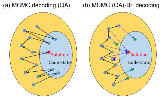
Figure 11: Schematic diagrams illustrating two modes that optimize (a) MCMC decoding (and QA) and (b) MCMC(QA)-BF hybrid decoding. The large and small ellipses indicate the search space and the code-state space, respectively. Blue circles indicate the sampled state by the MCMC or QA sampler. Green circles indicate the decoded states by the BF decoding. The red circle designates the correct code-state. Black solid arrows indicate the transitions to the following samples. Blue broken arrows indicate the BF decoding.

V.2 Spin-flipping mechanism and decoding cost

The above discussions did not discuss the mechanism for choosing the spins to be flipped at each iteration or the decoding cost of the BF algorithm. In concluding this paper, we would like to discuss these points briefly. Spin-flipping mechanisms are free to choose from several strategies. For example, only the most suitable spin chosen based on the inversion functions $\varDelta_{k}^{\left(X\right)}\left(\boldsymbol{x}\right)$’s estimated by the current decision $\boldsymbol{x}$ can be flipped. Alternatively, several spins chosen based on $\varDelta_{k}^{\left(X\right)}\left(\boldsymbol{x}\right)$’s can be flipped together. These are called the single-spin flipping and the multi-spin flipping strategies, respectively. In this classification, MCMC decoding algorithm belongs to the single-spin flipping strategy, while our BF decoding algorithm belongs to the multi-spin flipping strategy. Note that the BF decoding algorithm consists of two operations: evaluating the inversion function $\varDelta_{k}^{\left(BF\right)}\left(\boldsymbol{x}\right)$ and determining spins to be flipped. The inversion function $\varDelta_{k}^{\left(BF\right)}\left(\boldsymbol{x}\right)$ for each spin $k$ is computed at once from the current $\boldsymbol{x}$ by matrix multiplication. Subsequent sign evaluation for each element of $\varDelta_{k}^{\left(BF\right)}\left(\boldsymbol{x}\right)$ determines which spins are flipped together.

We can see from Fig.2 that more edges are connected to VNs in the weight-3 syndromes ($d_{v}=K-2$) than in the weight-4 syndromes ($d_{v}\leq 4$). Thus, each spin variable affects more syndromes in the weight-3 syndrome than in the weight-4 syndrome, and conversely, each spin variable is determined from more syndromes in the weight-3 syndrome than in the weight-4 syndrome. Consequently, when using the weight-3 syndrome, one must compute the sum of products of data distributed globally across many spins to decide whether to invert each spin. In contrast, when using the weight-4 syndrome, it is sufficient to compute the sum of products of data distributed over at most eight adjacent spins to determine whether to invert each spin. Such a global reduction operation to compute the inversion function, which occurs when using the weight-3 syndrome in the BF decoding algorithm, require more cost, but can accelerate the correction of errors in each spin-flip operation. On the other hand, the matrix multiplication required for calculating $\varDelta_{k}^{\left(BF\right)}\left(\boldsymbol{x}\right)$ can be easily performed and benefits from parallel computing techniques as well as hardware engines that calculate matrix sum products, such as GPUs and vector processing engines developed for machine learning. Note that this provides practical merit of choosing weight-3 syndrome for syndrome $s_{i}\left(\boldsymbol{x}\right)$ in $\varDelta_{k}^{\left(BF\right)}\left(\boldsymbol{x}\right)$ (Eq.(43)). In fact, comparing the computation times of the MCMC and MCMC-BF hybrid decoding shown in Fig.9, the computation time of MCMC-BF hybrid decoding was one-fifth of that of the MCMC decoding on the Mathematica platform. Although the computational cost depends on the algorithm used and the software or hardware platforms on which the calculations were performed, this result suggests that the MCMC-BF hybrid decoding is more efficient than MCMC decoding alone.

We don’t discuss the decoding cost in this paper in further detail because it is beyond the scope of this paper. We recall that this paper aims to demonstrate the validity of BF decoding as a second-stage decoder of a first-stage stochastic decoder, such as a QA device, in two-stage hybrid decoding. Since the development of QA devices is ongoing, it is not easy to demonstrate our BF decoding algorithm as a second-stage decoder of an actual QA device. Instead, the potential for BF decoding was demonstrated using a classical MCMC sampler in the first stage decoding. We believe that the present result is highly dependent on the property of the BF decoding algorithm, not the MCMC sampler. Furthermore, our result is consistent with the general belief that two decoding algorithms based on different mechanisms can be used together to solve problems that cannot be solved by either one alone. We believe that our BF decoding algorithm is promising for correcting errors in the readouts of QA devices due to measurement errors as well as dynamic errors that may be encountered during QA.

VI Conclusions

This study discussed practical methods for correcting errors in the readout of the spins in the SLHZ systems. Given the close relationship between the SLHZ system and the classical LDPC codes associated with the AWGN channel model, classical decoding techniques for LDPC codes are expected to provide noise immunity for the SLHZ system. To confirm this expectation, we conducted a classical simulation using MCMC sampling. We proposed a BF decoding algorithm based on majority voting, which is much simpler than the standard BP algorithm. We demonstrated that the BF decoding algorithm provides good protection against i.i.d. noise in the spin readout of the SLHZ system and is as efficient as the BP decoding algorithm. Using a classical MCMC sampler, we simulated stochastically sampled spin readouts on the SLHZ system to investigate the performance of BF decoding. We have shown that BF decoding can correct errors in the simulated readouts. This implies that the SLHZ system exhibits intrinsic fault tolerance when collaborating with the BF decoding against a broader range of noise models. Our observation is quite reasonable if we note that stochastic sampling followed by error correction can be identified as a two-stage hybrid decoding algorithm. Furthermore, controlling the annealing parameters in the first-stage sampler is essential to obtain the correct code-state efficiently. Particular attention should be given to finding the optimal annealing parameters, as they may largely depend on whether we perform decoding for the sampled readout or not.

Since our demonstration used readouts stochastically sampled by a classical method, specifically MCMC sampling, we are not fully convinced that the BF decoding algorithm is also valid for readouts obtained through QA of the SLHZ system. Further research is needed to assess how effectively the QA of the SLHZ system performs when used collaboratively with BF decoding under realistic laboratory conditions. Nevertheless, we believe that most of our insights stem from the intrinsic nature of BF decoding and are applicable regardless of the stochastic sampling mechanism employed in the initial stage. For example, if measurement error is the primary source of error in the spin readout of the SLHZ system, our BF decoding algorithm offers a straightforward solution to mitigate it. Additionally, it is reasonable to propose that a two-stage hybrid computation combining QA and post-readout BF decoding may address issues that neither method can solve independently. Our research also emphasizes the importance of adequately selecting decoding algorithms to exploit the potential of fault tolerance inherent in SLHZ systems.