Effects of fractional diffraction on nonlinear phase transitions and stability of dark solitons and vortices
Abstract
The wave propagation under the action of fractional diffraction has recently drawn increasing attention in nonlinear optics. Here, we address the effect of fractional diffraction on the existence, phase transitions, and stability of dark solitons (DSs) and vortices in parity-time () symmetric graded-index waveguide with self-defocusing nonlinearity. The DSs and vortices are produced by numerical solution of the corresponding one- and two-dimensional fractional nonlinear Schrödinger equations. We show that solution branches of fundamental and higher-order DSs collide pair-wise (merge) and disappear with the increase of the gain-loss strength, revealing nonlinear phase transitions in the waveguide. Numerically identifying the merger points, we demonstrate effects of the fractional diffraction on the phase transition. The phase transition points determine boundaries of existence regions for the DSs and vortices. The stability of the DSs and vortices is studied by means of the linearization with respect to small perturbations. Direct simulations of perturbed evolution corroborate their stability properties predicted by the analysis of small perturbations.
1 Introduction
Dark solitons (DSs) feature localized dips on a modulationally stable continuous wave (or extended finite-width) background [1]. The DSs are more stable than their bright counterparts against noise perturbations and are less susceptible to environmental disturbances. Thus, DSs offer various applications to optical communications and sensing, and are objects of basic interest to nonlinear optics in general [2, 3, 4].
The topic of symmetry started in the form of non-Hermitian quantum mechanics [5, 6, 7], where it was found that complex potentials obeying the symmetry could exhibit all-real spectra. The increase of the strength of the imaginary part of the complex potential leads to a phase transition in the respective linear system at a critical value of the strength, the spectrum acquiring complex eigenvalues above the critical value. The concept had later spread out to optics [8, 9], where the -symmetry is built as a combination of gain and loss elements which are mirror images of each other [10]. In nonlinear optics, -symmetric solitons are accessible in a wide variety of nonlinear optical platforms [11, 12, 13]. In such a setting, dark solitons were predicted in the framework of the nonlinear Schrödinger equation (NLSE) with the -symmetric potential [14]. DSs also exist in coupled NLSEs, including models of -symmetric dual-core optical couplers [15] (similar to bright solitons predicted in the same system [16, 17]). In particular, DS dynamics was studied in -symmetric nonlinear directional couplers with third-order and intermodal dispersions, where phase-controlled switching dynamics with excellent efficiency was demonstrated with a very low critical power [18]. Furthermore, the creation of dark solitons and vortex solitons were proposed in a cold-atom system with linear and nonlinear -symmetric potentials [19, 20, 21, 22, 23, 24, 25, 26, 27].
Recently, optical solitons have been investigated in the framework of fractional NLSEs (FNLSEs) [28, 29, 30, 31], which include the effective fractional diffraction or dispersion represented by the Riesz fractional derivative with the respective Lévy index (LI). The linear fractional Schrödinger equation (FSE) originates from fractional-dimensional quantum mechanics [32, 33]. The derivation was based on the Feynman’s path integration, where the superposition of the motions was taken along paths that correspond not to the usual Brownian random walks, but to trajectories built by Lévy flights with the respective LI.
FSE can be emulated in classical optics, as proposed by Longhi [34], using an optical cavity incorporating two lenses and a phase mask. The lenses perform direct and inverse Fourier transforms of the light beam with respect to the transverse coordinate(s), while the phase mask creates the phase structure corresponding to the action of the fractional diffraction. Then, the continuous FSE is introduced by averaging over many cycles of circulation of light in the cavity. Another possibility for the realization of FSE in optics is provided by the transmission of light pulses in the temporal domain, with an effective fractional group-velocity dispersion acting on femtosecond laser pulses [35].
In the context of optics, it is natural to include nonlinearity in FSE, leading to fractional NLSE, where the prediction of fractional optical solitons have drawn much interest [36, 37, 38, 39, 40, 41, 42, 43, 44, 45, 46, 47]. Furthermore, fractional diffraction was used to manipulate the Airy beam dynamics [48, 49]. Earlier, fractional NLSEs with -symmetric potentials were addressed, where symmetric and antisymmetric solitons and ghost states with complex-conjugate propagation constants were demonstrated [50, 51], as well as their two-dimensional counterparts [52].
Previous studies on factional NLSEs focused primarily on properties of bright solitons, while the existence and stability of non-Hermitian dark solitons and vortices have not been fully investigated. In this work, we address fractional DSs and vortices in one- and two-dimensional models of the nonlinear waveguide with fractional diffraction, characterized by LI and the -symmetric potential. We identify families of fractional DSs and vortices, and find branches of these modes that collide in pairs and disappear at the points of the nonlinear phase transition (which is different from the above-mentioned phase transition of breaking the real spectrum in linear -symmetric systems). We examine the effect of the fractional diffraction on the phase transitions and stability of the fractional DSs and vortices, by producing stationary solutions for them and performing their linear-stability analysis. We also consider the perturbed evolution of stable and unstable fractional DSs and vortices, which confirms the predictions of the linear-stability analysis.
2 The model and numerical methods
2.1 The model
Our model addresses the propagation of light in the fractional diffraction medium governed by the dimensionless FNLSE [50, 52]
| (1) |
where variables and represent the normalized propagation length and coordinate in the transverse direction, respectively, and the normalized nonlinearity coefficient corresponds to the self-defocusing sign of the cubic term. The fractional diffraction with LI is defined as the above-mentioned Riesz derivative:
| (2) |
It is built as a nonlocal operator, produced by the juxtaposition of the direct and inverse Fourier transforms, with fractional differentiation proper represented by factor in the Fourier space. Normally, LI takes values , the limit of corresponding to the canonical (non-fractional) Schrödinger equation, with operator (2) reducing to the usual second derivative. Actually, the constraint of is imposed in the one-dimensional FNLSE with the self-focusing sign of the cubic nonlinearity, as in that case the model demonstrates the critical and supercritical collapse at and , respectively. However, the collapse does not take place if the nonlinearity is self-defocusing, which is the case in Eq. (1), hence values of may be possible too.
Even and odd functions and in Eq. (1) are the real and imaginary parts of the -symmetric potential, which represent, respectively, the graded-index structure and the balanced distribution of the gain and loss [53, 54, 55]. In this work, we adopt them in the natural form of
| (3) |
where is the width of the corresponding harmonic-oscillator (HO) potential, and is the modulation strength of the gain and loss. Note that, in the conservative fractional system, with , the conservation of the integral power, , is a result of the direct substitution of the expression for , taken as per Eq. (1).
Setups that realize the nonlinear phase transitions in optical systems with fractional diffraction were designed on the basis of the Fabry-Perot resonator, with two convex lenses and two phase masks inserted into it, the fractional diffraction proper being implemented in the Fourier space [34]. The cubic nonlinearity is incorporated by placing a nonlinear optical material between the edge mirror and the closest lens. As for the symmetry, its straightforward realization is provided by adding a balanced pair of gain and loss elements to the resonator [10].
We look for fractional DSs with a real propagation constant as stationary solutions to Eq. (1),
| (4) |
where may be split in the real and imaginary parts. The substitution of this expression into Eq. (1) yields the stationary equation
| (5) |
Families of DSs are characterized by the integral power (norm), which is a dynamical invariant of Eq. (1), defined as
| (6) |
(formally, it diverges, but in reality it is convergent for a finite-length spatial domain).
2.2 The solution method for DSs (dark solitons)
We seek for fractional DS solutions to Eq. (5) employing the Newton conjugate-gradient (NCG) method [56], with a fixed propagation constant and soliton power. Accordingly, Eq. (5) is rewritten as
| (7) |
where . Here, the boundary condition is at edges of the spatial domain, which is taken as . As said above, the propagation constant is considered as a parameter with a fixed value, whereas the solution for is generated by means of the Newton’s iterations. To solve Eq. (5), we iteratively update the approximation for as
| (8) |
where is a small error term. Then we substitute this expression in Eq. (5) and expand it around , which yields
| (9) |
where is the linearization operator of Eq. (7) evaluated with the approximate solution . The updated term is obtained from the linear Newton-correction equation,
| (10) |
where
| (11) |
and stands for the complex conjugate. As is not self-adjoint, we apply to it the adjoint operator of and thus turn it into the following equation:
| (12) |
In the framework of this scheme, Eq. (12) can be solved directly by dint of conjugate-gradient iterations, which yields families of DS.
2.3 The linear stability analysis
To investigate the stability of the DSs, we apply the standard linearization procedure, adding a small perturbation to the unperturbed solution:
| (13) |
where and are components of the perturbation eigenmode, with , and is the respective eigenvalue. The stationary solution is stable if all eigenvalues have .
Substituting ansatz (13) in Eq. (1) and linearizing it with respect to the perturbation, we arrive at the linear eigenvalue problem:
| (14) |
3 Results and discussion
3.1 Families of the fractional DSs and the nonlinear transition
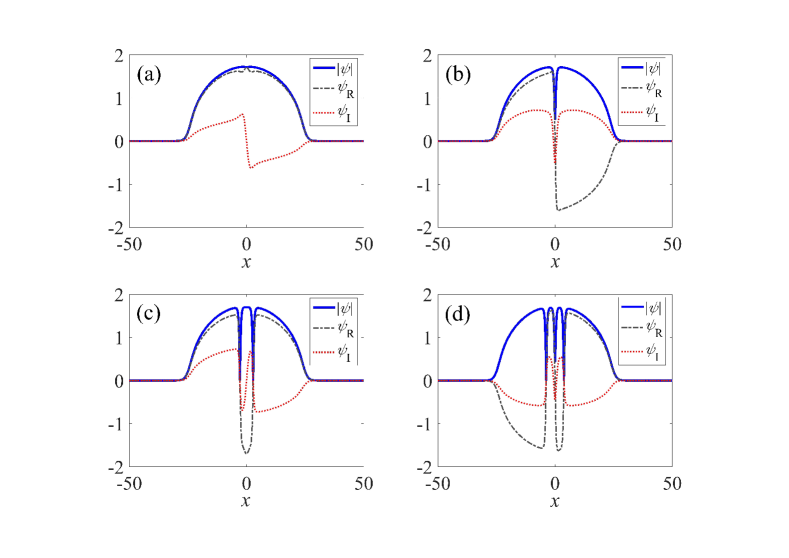
As generic numerically obtained examples, a fundamental DS (FDS) and high-order (multiple) ones are represented in Fig. 1 for a fixed propagation constant , LI , the modulation strength of the gain-loss distribution and the width of the HO potential . Figure 1(a) shows the real and imaginary parts of the fractional FDS, which are even and odd functions of due to the symmetry. The parities of the real and imaginary parts alternate in the first-, second-, and third-order higher-order fractional DSs (designated, severally, as 1DS, 2DS, and 3DS modes), as shown in Figs. 1(b), (c) and (d), respectively.
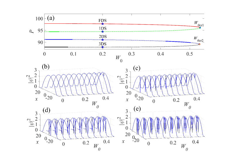
Next, we consider the effect of the gain-loss modulation strength on the stability of the fractional DSs. To this end, the numerically found dependence of the DS’s power on the gain-loss modulation strength is shown in Fig. 2(a) for the fixed LI value . The diagram encompasses pairwise branches of the DS families, with the pair of the FDS and 1DS branches merging at the first critical point, , and the 2DS – 3DS pair merging at the second critical point, . These pairwise mergers represent nonlinear phase transition in the fractional-diffraction medium. Further, it is seen that the fractional FDSs are stable in their entire existence domain, while the stability regions of the higher-order fractional DSs are piecewise. The dependence of the DS shapes on the gain-loss modulation strength are presented in Figs. 2(b)-(e). The shapes of fractional FDSs and 1DSs converge to a similar profile as increases, as shown in Figs. 2(b) and (c), and eventually become identical at the phase transition points. Actually, the fractional FDS and 1DS possess the same envelope shapes, but opposite real and imaginary parts at the phase transition points. A similar scenario takes place for the 2DS and 3DS branches, as shown in Figs. 2(d) and (e).
3.2 The nonlinear phase transition and stability of the fractional DSs (dark solitons)
To investigate the effect of the fractional diffraction on the existence and stability of DSs, the dependence of the branches of the DS families and phase transition points on the fractional diffraction is thoroughly analyzed by means of computing the fractional DS solutions and their stability spectra on LI in the interval .
| Lévy index | Lévy index | ||||||
|---|---|---|---|---|---|---|---|
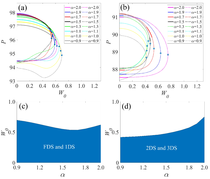
The systematic results for the different values of LI are summarized in Fig. 3, in which stable and unstable families are represented by the solid and dashed segments, respectively, in Figs. 3(a) and (b), respectively. Figure 3(a) shows that, as above, the fractional FDSs are stable in their entire existence domain for a relatively weak fractionality (), while unstable fractional FDSs occur in a narrow region near the phase transition points for stronger fractionality (). With the increase of the fractionality, stable regions of the higher-order DSs shrink and eventually disappear. The most pronounced difference is observed for 2DSs, which are stable in a narrow region near the phase transition points for and in Fig. 3(b).
To quantify the effect of the fractional diffraction on the nonlinear phase transitions, we address the dependence of the corresponding critical values of on LI. Figures 3(c) and 3(d) show as a function of LI. Note that the phase-transition points constitute existence boundaries for the fractional DSs. It is noteworthy that, different from the fixed positions of nonlinear phase transitions in non-fractional models [14], the existence domains of the FDSs and 1DSs first shrink and then gradually expand with the increase of LI, as shown in Fig. 3(c). On the other hand, the existence domain for the 2DSs and 3DSs is monotonically expanding in Fig. 3(d). We identified the boundaries of the existence domains for the fractional DSs by calculating the critical values of and for the nonlinear phase transitions, which are summarized in Table 1 for different LI values, ranging from to with a step of .
3.3 The evolution of the fractional DSs (dark solitons)
To corroborate the predictions of the linear-stability analysis, we have performed numerical simulations of Eq. of the perturbed evolution of the fractional DSs of Eq. (1). Typical examples are presented in Figs. 4 and 5 for fixed values of , , and .
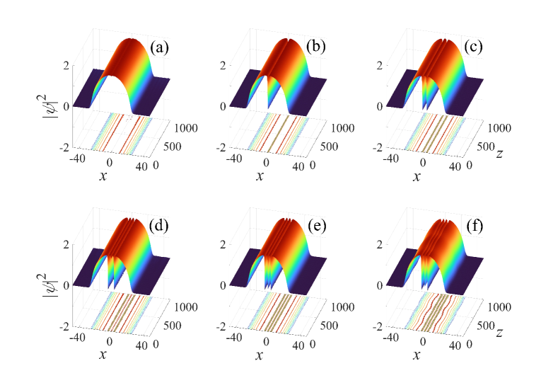
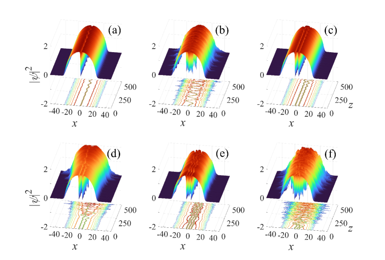
Representative examples of possible stable dynamics of the fractional FDSs and high-order dark solitons are shown in Fig. 4. Linearly stable FDSs and 1DSs are perturbed by random noise for at , as shown in Figs. 4(a) and (b). The results confirm that the linearly stable FDS and 1DS, as predicted by the linear-stability analysis, remain robust, at least, up to . The linearly stable 2DSs exist in two different regions, as shown in Fig. 2(a), therefore we separately examine the stability and evolution of the 2DSs at and . It is seen in Figs. 4(c) and (d) that, at least up to , the linearly stable 2DSs indeed remain stable in the course of the perturbed propagation. The evolution results displayed in Figs. 4(e) and 4(f) confirm that, under the noise perturbation, the stable fractional 3DSs also survive as stable states.
To demonstrate the unstable evolution, fractional DSs, which are predicted to be unstable by the linear-stability analysis, are also disturbed by random noise. Figure 5 displays typical examples of the evolution of unstable 1DSs [panels Figs. 5(a) and (b)], 2DSs [panels Figs. 5(c) and (d)], and 3DSs [panels Figs. 5(e) and (f)]. The evolution of the unstable fractional DSs demonstrates spontaneous onset of oscillations and displacement of the center.
3.4 The two-dimensional system
Finally, we consider the two-dimensional -symmetric potential with a real part
| (16) |
which represents the two-dimensional HO trap, and the odd imaginary part
| (17) |
To investigate effects of the fractional diffraction on the nonlinear phase transitions and stability of two-dimensional DSs, the dependence of branches of two-dimensional FDSs, single-vortex, and vortex-dipole families on the diffraction fractionality are analyzed by computing the solutions and respective stability spectra for a fixed HO width, , and LI ranging from to . Here, the boundary condition is at edges of the spatial domain, which is taken as .
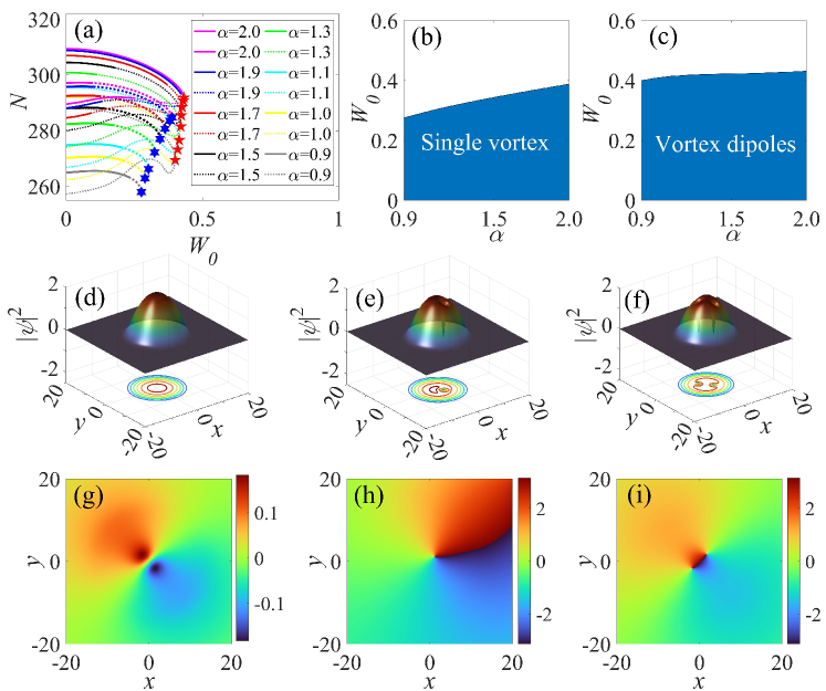
The power curves for the families of two-dimensional FDS, single vortex and vortex dipole (i.e., vortex-antivortex bound states) are plotted in Fig. 6(a), where the branches disappear at the respective critical values of . Note that the two-dimensional FDSs are stable in their entire existence domains of existence solely for (the usual NLSE with the non-fractional diffraction). In the case of the fractional diffraction () instability of two-dimensional FDSs occurs. Thus, the stability range for the two-dimensional FDSs gradually shrinks with the increase of the fractionality (decrease of LI). In contrast, the stability range for the single vortex gradually expands with the decrease of LI. Vortex dipoles are stable only in narrow subregions of the their existence domain and become completely unstable as .
| Lévy index | Lévy index | ||||||
|---|---|---|---|---|---|---|---|
The boundaries of the existence domain of the two-dimensional FDSs and vortex dipoles, as well as the the single vortex are obtained by calculating the respective critical values and at the nonlinear phase transition points. These critical values are summarized in Table 2, which demonstrates that the critical values of decrease as the fractionality increases. This means that the existence domains of the two-dimensional FDSs, single vortices, and vortex dipoles shrink with the decrease of LI, as shown in Fig. 6(b) and (c). Representative examples of stable two-dimensional FDS, single vortex and vortex dipole are displayed, respectively, in Figs. 6(d), (e) and (f), along with their phase profiles in Figs. 6(g), (h) and (i).
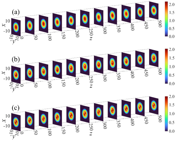
Next, we examine the stability and evolution of the two-dimensional FDSs, single vortices, and vortex dipoles by means of direct simulations of their perturbed evolutions. The robust propagation of the two-dimensional FDS at parameters corresponding to the stable region identified in Fig. 6(a) is indeed demonstrated by the simulations performed in the presence of perturbations. As shown in Fig. 7(a), the perturbed propagation remains stable at least up to under the action of random initial perturbations with a relative amplitude of . Figures 7(b) and (c) corroborate the robust propagation of the stable single vortex and vortex dipole.
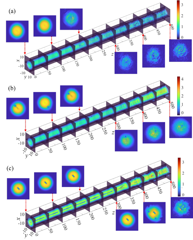
On the other hand, examples of the unstable evolution of the two-dimensional FDS, single vortex, and vortex dipole are presented in Fig. 8. The simulations, their instability, as predicted by the linear-stability analysis (the onset of the instability, leading to emergence of “turbulence", is readily observed even in the absence of random perturbations). Figure 8 (a) shows that the unstable two-dimensional FDS survives as a quasi-stable mode at the early stage of the evolution (), which is followed by the onset of conspicuous instability. Figs. 8(b) and (c) show that the unstable vortex dipole survives as a quasi-stable mode up to ; then, it starts to rotate and eventually collapses.
4 Conclusion
In the present work, we have produced numerical solutions for the one- and two-dimensional fractional FDSs (fundamental-dark-soliton), as well as one-dimensional higher-order DS (dark-soliton), two-dimensional single-vortex, and vortex-dipole families. The analysis reveals the nonlinear phase transitions (the merger of pairs of branches representing different families), which suggests possibility for new experiments in fractional nonlinear optical systems. The fractional diffraction produces a significant effect on the nonlinear phase transition, reflected in the dependence of parameters of the respective merger points on the LI (Lévy index). The existence and stability regions for the fractional DSs, single vortices, and vortex dipoles have been identified. Direct simulations of the perturbed evolution of these modes fully agree with the predictions of the linear-stability analysis. The complex stability patterns of the fractional DSs and vortex dipoles uncover multiple effects of the fractional diffraction, symmetry, and nonlinearity.
Extension of the present analysis may address vortex solitons with higher topological charges, vortex rings and other forms of two-dimensional DS structures.
Funding National Natural Science Foundation of China (11805141); Shanxi Province Basic Research Program (202203021222250, 202303021211185); Israel Science Foundation (grant No. 1695/22).
Disclosures The authors declare no conflicts of interest.
Data Availability Statement Data underlying the results presented in this paper are not publicly available at this time but may be obtained from the authors upon reasonable request.
References
- [1] Y. S. Kivshar and B. Luther-Davies, “Dark optical solitons: physics and applications,” Phys. Rep. 298(2-3), 81–197 (1998).
- [2] S. Yang, Q. Y. Zhang, Z. W. Zhu, et al., “Recent advances and challenges on dark solitons in fiber lasers,” Opt. Laser Technol. 152(8), 108116 (2022).
- [3] W. S. Zhao and E. Bourkoff, “Generation, propagation, and amplification of dark solitons,” J. Opt. Soc. Am. B 9(7), 1134–1144 (1992).
- [4] L. W. Zeng, J. C Shi, Jiawei Li, et al., “Dark soliton families in quintic nonlinear lattices,” Opt. Express 30(23), 42504–42511 (2022).
- [5] C. M. Bender, S. Boettcher, and P. N. Meisinger, “-symmetric quantum mechanics,” J. Math. Phys. 40(5), 2201–2229 (1999).
- [6] A. Mostafazadeh, “Pseudo-Hermiticity versus symmetry: The necessary condition for the reality of the spectrum of a non-Hermitian Hamiltonian,” J. Math. Phys. 43(1), 205–214 (2002).
- [7] C. M. Bender and D. W. Hook, “-symmetric quantum mechanics,” Rev. Mod. Phys. 96(4), 045002 (2024).
- [8] R. El-Ganainy, K. G. Makris, D. N. Christodoulides, et al., “Theory of coupled optical -symmetric structures, ” Opt. Lett. 32(17), 2632–2634 (2007).
- [9] R. El-Ganainy, K. G. Makris, M. Khajavikhan, et al., “Non-Hermitian physics and symmetry,” Nat. Phys. 14(1), 11–19 (2018).
- [10] C. E. Rüter, K. G. Makris, R. El-Ganainy, et al., Observation of parity-time symmetry in optics,” Nat. Phys. 6(3), 192–195 (2010).
- [11] V. V. Konotop, J. K. Yang, and D. A. Zezyulin, “Nonlinear waves in -symmetric systems,” Rev. Mod. Phys. 88(3), 035002 (2016).
- [12] S. V. Suchkov, A. A. Sukhorukov, J. H. Huang, et al., “Nonlinear switching and solitons in -symmetric photonic systems,” Laser Photon. Rev. 10(2), 177–213 (2016).
- [13] L. Feng, R. El-Ganainy, and L. Ge, “Non-Hermitian photonics based on parity-time symmetry,” Nat. Photon. 11(12), 752–762 (2017).
- [14] V. Achilleos, P. G. Kevrekidis, D. J. Frantzeskakis, et al., “Dark solitons and vortices in -symmetric nonlinear media: from spontaneous symmetry breaking to nonlinear phase transitions," Phys. Rev. A 86(1), 013808 (2012).
- [15] Y. V. Bludov, V. V. Konotop, and B. A. Malomed, “Stable dark solitons in -symmetric dual-core waveguides,” Phys. Rev. A 87(1), 013816 (2013).
- [16] R. Driben and B. A. Malomed, “Stability of solitons in parity-time-symmetric couplers,” Opt. Lett. 36(22), 323–4325 (2011).
- [17] N. V. Alexeeva, I. V. Barashenkov, A. A. Sukhorukov, et al., “Optical solitons in -symmetric nonlinear couplers with gain and loss,” Phys. Rev. A 85(6), 063837 (2012).
- [18] D. K. Mahato, A. Govindarajan, and A. K. Sarma, “Dark soliton steering in -symmetric couplers with third-order and intermodal dispersions,” J. Opt. Soc. Am. B 37(11), 3443–3452 (2020).
- [19] D. A. Zezyulin, I. V. Barashenkov, and V. V. Konotop, “Stationary through-flows in a Bose-Einstein condensate with a PT-symmetric impurity,” Phys. Rev. A 94(6), 063649 (2016).
- [20] B. A. Malomed and D. Mihalache, “Nonlinear waves in optical and matter-wave media: a topical survey of recent theoretical and experimental results,” Rom. J. Phys. 64, 106 (2019).
- [21] L. W. Dong and C. M. Huang, “Vortex solitons in fractional systems with partially parity-time-symmetric azimuthal potentials,” Nonlinear Dyn. 98, 1019–1028 (2019).
- [22] G. M. Li, A. Li, S. J. Su, et al., “Vector spatiotemporal solitons in cold atomic gases with linear and nonlinear symmetric potentials,” Opt. Express 29(9), 14016–14024 (2021).
- [23] Y. Zhao, H. J. Hu, Q. Q Zhou, et al., “Three-dimensional solitons in Rydberg-dressed cold atomic gases with spin-orbit coupling,” Sci. Rep. 13(1), 18079 (2023).
- [24] B. B. Li, Y. Zhao, S. L. Xu, et al., “Two-dimensional gap solitons in parity-time symmetry Moiré optical lattices with Rydberg-Rydberg interaction,” Chin. Phys. Lett. 40(4), 044201 (2023).
- [25] S. L. Xu, T. Wu, H. J. Hu, et al., “Vortex solitons in Rydberg-excited Bose-Einstein condensates with rotating PT-symmetric azimuthal potentials,” Chaos, Solitons Fractals 184, 115043 (2024).
- [26] Y. Zhao, Q. H. Huang, T. X. Gong, et al., “Three-dimensional solitons supported by the spin–orbit coupling and Rydberg-Rydberg interactions in PT-symmetric potentials,” Chaos, Solitons Fractals 187, 115329 (2024).
- [27] S. L. Xu, J. H. Li, Y. H. Hou, et al., “Vortex light bullets in Rydberg atoms trapped in twisted PT-symmetric waveguide arrays,” Phys. Rev. A 110(2), 023508 (2024).
- [28] B. A. Malomed, “Optical solitons and vortices in fractional media: a mini-review of recent results,” Photonics 8(9), 353 (2021).
- [29] B. A. Malomed, “Basic fractional nonlinear-wave models and solitons,” Chaos 34, 022102 (2024).
- [30] P. G. Kevrekidis and J. Cuevas-Maraver, eds. Fractional Dispersive Models and Applications (Springer, 2024).
- [31] D. Mihalache, “Localized structures in optical media and Bose-Einstein condensates: an overview of recent theoretical and experimental results,” Rom. Rep. Phys. 76(2), 402 (2024).
- [32] N. Laskin, “Fractional quantum mechanics and Lévy path integrals,” Phys. Lett. A 268(4-6), 298–305 (2000).
- [33] N. Laskin, “Fractional Schrödinger equation,” Phys. Rev. E 66(5), 056108 (2000).
- [34] S. Longhi, “Fractional Schrödinger equation in optics,” Opt. Lett. 40(6), 1117–1120 (2015).
- [35] S. L. Liu, Y. W. Zhang, B. A. Malomed, et al., “Experimental realisations of the fractional Schrödinger equation in the temporal domain,” Nat. Commun. 14(1), 222 (2023).
- [36] M. N. Chen, S. H. Zeng, D. Q. Lu, et al., “Optical solitons, self-focusing, and wave collapse in a space-fractional Schrödinger equation with a Kerr-type nonlinearity,” Phys. Rev. E 98(2), 022211 (2018).
- [37] X. K. Yao and X. M. Liu, “Off-site and on-site vortex solitons in space-fractional photonic lattices,” Opt. Lett. 43(23), 5749–5752 (2018).
- [38] L. W. Zeng and J. H. Zeng, “One-dimensional solitons in fractional Schrödinger equation with a spatially periodical modulated nonlinearity: nonlinear lattice,” Opt. Lett. 44(11), 2661–2664 (2018).
- [39] L. W. Dong, C. M. Huang, and W. Qi, “Nonlocal solitons in fractional dimensions,” Opt. Lett. 44(20), 4917–4920 (2019).
- [40] C. M. Huang and L. W. Dong, “Dissipative surface solitons in a nonlinear fractional Schrödinger equation,” Opt. Lett. 44(22), 5438–5441 (2019).
- [41] L. Li, H. G. Li, W. Ruan, et al., “Gap solitons in parity-time-symmetric lattices with fractional-order diffraction,” J. Opt. Soc. Am. B 37(2), 488–494 (2020).
- [42] M. Molina, “The fractional discrete nonlinear Schrödinger equation,” Phys. Lett. A 384(8), 126180 (2020).
- [43] X. Zhu, F. W. Yang, S. L. Cao, et al., “Multipole gap solitons in fractional Schrödinger equation with parity-time-symmetric optical lattices,” Opt. Express 28(2), 1631–1639 (2020).
- [44] P. F. Li, B. A. Malomed, and D. Mihalache, “Symmetry breaking of spatial Kerr solitons in fractional dimension,” Chaos, Solitons Fractals 132, 109602 (2020).
- [45] P. F. Li, R. J. Li, and C. Q. Dai.“Existence, symmetry breaking bifurcation and stability of two-dimensional optical solitons supported by fractional diffraction,” Opt. Express 29(3), 3193–3210 (2021).
- [46] C. Mejía-Cortés and M. I. Molina, “Fractional discrete vortex solitons,” Opt. Lett. 46(10), 2256–2259 (2021).
- [47] J. F. Wang, Y. Jin, X. G. Gong, et al., “Generation of random soliton-like beams in a nonlinear fractional Schrödinger equation,” Opt. Express 30(5), 8199–8211 (2022).
- [48] C. Tan, T. Lei, M. Zou, et al., “Manipulating circular Airy beam dynamics with quadratic phase modulation in fractional systems under some diffraction modulations and potentials,” Opt. Express 32(14), 25261–25275 (2024).
- [49] C. Tan, T. Lei, M. Zou, et al., “Generation and control of circular Airy solitons in fractional nonlinear optical systems under different modes,” Opt. Express 32(22), 38312–38326 (2024).
- [50] P. F. Li, B. A. Malomed, and D. Mihalache, “Symmetry-breaking bifurcations and ghost states in the fractional nonlinear Schrödinger equation with a -symmetric potential,” Opt. Lett. 46(13), 3267–3270 (2021).
- [51] M. Zhong, L. Wang, P. F. Li, et al., “Spontaneous symmetry breaking and ghost states supported by the fractional -symmetric saturable nonlinear Schrödinger equation,” Chaos 33(1), 013106 (2023).
- [52] M. Zhong and Z. Y. Yan, “Spontaneous symmetry breaking and ghost states in two-dimensional fractional nonlinear media with non-Hermitian potential,” Commun. Phys. 6(1), 92 (2023).
- [53] W. H. Renninger and F. W. Wise, “Optical solitons in graded-index multimode fibres,” Nat. Commun. 4(1), 1719 (2013).
- [54] Y. L. Shuai, Z. X. Deng, H. Z. Li, et al., “Peregrine soliton emits dispersive waves within graded-index multimode fibers without higher-order dispersion,” J. Opt. Soc. Am. B 41(6), 1317–1323 (2024).
- [55] P. Parra-Rivas, Y. F. Sun, F. Mangini, et al., “Pure quartic three-dimensional spatiotemporal Kerr solitons in graded-index media,” Phys. Rev. A 109(3), 033516 (2024).
- [56] J. K. Yang, Nonlinear Waves in Integrable and Nonintegrable Systems (SIAM, 2010).