Fingerprint Matrix Concept for Detecting, Localizing and Characterizing Targets in Complex Media

Abstract

As waves propagate through a complex medium, they undergo multiple scattering events. This phenomenon is detrimental to imaging, as it causes a full blurring of the image beyond a transport mean free path. Here, we show how to detect, localize, and characterize any scattering target through the reflection matrix of the complex medium in which this target is embedded and thus hidden from direct view. More precisely, we introduce a fingerprint operator that contains the specific signature of the target with respect to its environment. Applied to the recorded reflection matrix, this operator provides a likelihood index of the target in any given state, despite the scattering fog induced by the surrounding environment. This state can be the target position for localization purposes, its shape for characterization, or any other parameter that influences the target response. Our concept is versatile and broadly applicable to different type of waves for which multi-element technology allows a reflection matrix to be measured. We demonstrate this here explicitly by performing different proof-of-concept experiments with ultrasound on targets buried inside a strongly scattering granular suspension, on lesion markers for clinical applications, and on the architecture of muscle tissue.

Introduction

With the emergence of multi-element technology, it has become possible to cope with the enormous complexity of disordered media for focusing waves through them or for imaging objects hidden behind them. This feat has been been realized in acoustics, using the concept of the time reversal mirror ¹ or, in optics, using wave-front shaping techniques ². More fundamentally, a matrix formalism is particularly appropriate when wave fields can be controlled by transmission ^{3, 4} and/or reception ^{5, 6} arrays of independent elements. Since an inhomogeneous medium can be treated as one realization of a random process, some aspects of random matrix theory and basic concepts from scattering theory have been fruitfully applied to wave control or imaging through complex media ^{7, 8, 9}. In particular, transmission eigenchannels have been shown to provide a properly designed combination of incident waves that can be fully transmitted through a disordered medium ^{10, 11, 12}. The reflection eigenchannels, on the other hand, have been shown to focus on bright point-like targets embedded in a disordered medium, provided that the disorder is not too strong ^{13, 14}. For more complex targets, these methods are not adapted since the one-to-one association between each eigenstate and each target is no longer verified in the general case ^{15, 16}. Much progress has also been made using the reflection matrix ^{17, 18}, the time-reversal matrix ^{19, 20} or the distortion operator ^{21, 22} for imaging, in particular, to compensate the effects of disorder ^{23, 24, 25, 26, 27}. All currently available techniques, however, face the key challenge that, in the regime of strong multiple scattering, such a compensation becomes close to impossible.

In the present article, we address this outstanding challenge with an approach that is not based on compensating the effect of disorder, but rather by detecting correlations in the scattering of waves that survive even for very thick disordered media. The starting point for this approach is the following scattering invariant operator that has been constructed based on the matrix product $\mathbf{T}\times\mathbf{T}_{0}^{{\dagger}}$ between the transmission matrix of a disordered medium $\mathbf{T}$ and a matrix $\mathbf{T}_{0}$ of a homogeneous reference medium ²⁸. The associated eigenstates of this operator have been shown to be ‘scattering invariant modes’ in the sense that they exhibit a transmitted field pattern behind a disordered medium that is identical to that of purely ballistic waves, independent of the multiple scattering events endured by the waves inside the medium.

While the scattering invariant modes are thus input states that are transmitted through a disordered medium as through free (or homogeneous) space, we need something different here: what we are looking for in the context of target detection are input states that are reflected from a target embedded inside a disordered medium in the same way as from a target embedded in free (or homogeneous) space. Correspondingly, the operator $\mathbf{\Gamma}$ that we introduce here is defined as the matrix product ${\color[rgb]{0,0,0}\mathbf{\Gamma}}=\mathbf{R}\times\mathbf{R}_{0}^{\dagger}$ between a measured reflection matrix $\mathbf{R}$ of a disordered medium potentially hiding a target and the conjugate transpose of a reference matrix $\mathbf{R}_{0}$ associated with a target in absence, this time, of any disordered environment. This matrix $\mathbf{R}_{0}$ can be parametrized by a target state vector $\mathbf{q}$ whose coefficients account for the position, size and shape of the target alone. We thus refer to $\mathbf{R}_{0}(\mathbf{q})$ as the fingerprint matrix. In practice, $\mathbf{R}_{0}(\mathbf{q})$ can, e.g., be determined by measuring the reflection matrix of a known target in free space and by shifting its position to arbitrary values through the knowledge of the free-space Green’s function (Methods). Alternatively, also fully computational approaches to evaluate $\mathbf{R}_{0}(\mathbf{q})$ for different target shapes and sizes are viable as we will show below. In all these cases, the key insight is the following: the more closely the position, size or shape of the target in the fingerprint matrix $\mathbf{R}_{0}(\mathbf{q})$ match their true values realized in the experimentally measured matrix $\mathbf{R}$, the higher the correlations between these two matrices will be - allowing us to determine the target properties through an optimization problem. Our concept is therefore extremely versatile since the fingerprint matrix can be designed as a function of the experimental situation, and can be applied to any kind of waves, provided that a measurement of the reflection matrix is possible.

To illustrate the power of the fingerprint operator concept and its wide flexibility, we will present three different ultrasound experiments. The first implementation will tackle the extremely challenging scenario of elastic spheres buried inside a strongly scattering dense granular suspension up to a depth of five transport mean free paths. We will show how the fingerprint operator allows us to selectively detect and localize these spheres of different diameters despite a strongly predominant diffusive fog. In a second experiment, we will demonstrate how this idea can be also useful in a weaker scattering regime and easily transposed to more complex objects generally used in clinical applications for marking biopsy sites and suspicious lesions in breast tissue. In a third experimental demonstration, we will show how the fingerprint operator can be leveraged for characterizing the complex medium itself. As a proof-of-concept, we will use our approach to map the fiber architecture within muscle tissue. In the last part of the manuscript, we will discuss the potential of the fingerprint operator both from a fundamental side and an applied side in various fields of wave physics.

Results

Multiple scattering as a nightmare for imaging

The first experiment consists in the ultrasound imaging of two metal spheres embedded into a granular suspension consisting of randomly packed glass beads (diameter $\varnothing\simeq$ 300-315 $\mu$m) immersed in water with a packing density of 60% ²⁹ (Fig. 1a). The spheres have diameters $d_{1}=10$ mm and $d_{2}=8$ mm. Their centers $\mathbf{r}_{1}$ and $\mathbf{r}_{2}$ are positioned 9 and 7 mm below this granular suspension surface, respectively. The experimental procedure first consists in the acquisition of the reflection matrix using a two-dimensional array of 1024 transducers placed on top of the granular suspension surface into which the metal spheres are embedded (Methods). The reflection matrix is here acquired using a set of plane waves (Fig. 1b, Methods) over a 1.8-2.6 MHz frequency bandwidth. For each plane wave with incidence angles $\bm{\theta}_{\textrm{in}}=(\theta_{x},\theta_{y})$, the time-dependent reflected wave field $R(\bm{\mathrm{u}}_{\mathrm{out}},\bm{\theta}_{\textrm{in}},t)$ is recorded by each transducer $\bm{\mathrm{u}}_{\mathrm{out}}$ (Fig. 1c). This set of wave-fields forms a reflection matrix acquired in the plane wave basis, $\mathbf{R}_{\bm{\theta}\mathbf{u}}(t)=\left[R(\bm{\mathrm{u}}_{\mathrm{out}},\bm{\theta}_{\textrm{in}},t)\right]$. A Fourier transform can then be applied to the experimentally acquired reflection matrix to obtain its frequency-dependent counterpart, $\mathbf{R}_{\bm{\theta}\mathbf{u}}(f)=\int dt\mathbf{R}_{\bm{\theta}\mathbf{u}}(t)\exp\left(-j2\pi ft\right)$, with $f$ the frequency.

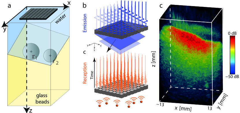
Figure 1: Multiple scattering fog. a, Experimental configuration: A 2D array of 1024 ultrasound transducers is used to detect two metal spheres that are embedded in strongly scattering glass beads below water. b, The reflection matrix is measured in the plane-wave basis ($\bm{\theta}_{\textrm{in}}$) in transmit. c, Each back-scattered wave field $R(\mathbf{u}_{\textrm{out}},\bm{\theta}_{\textrm{in}},t)$ is recorded on each transducer $\mathbf{u}_{\textrm{out}}$ of the probe. d, Volumetric visualization of the probed medium by projecting the intensity maximum of the confocal image obtained by a delay-and-sum beamforming applied to the recorded reflection matrix (a dynamic view of this is shown in Supplementary Movie 1). With this conventional imaging technique, the specular echo of the interface between water and the glass bead suspension largely predominates and the targets are completely invisible on the image.

A focused beamforming algorithm (Methods) is then applied to the reflection matrix to obtain a confocal image of the medium under investigation. The result is displayed in Fig. 1d. Although the image shows a strong specular echo at the surface of the granular suspension, the two spheres located beneath this surface are fully invisible on the image. Two reasons can be invoked to explain the failure of a standard imaging process in this experimental configuration:

1. First, the granular suspension is strongly scattering, as evidenced by the scattering mean free path $\ell_{s}\sim 1.8$ mm exhibited by ultrasonic waves in the frequency range of interest (Supplementary Section S1). Note that scattering by the glass bead packing is isotropic in the frequency range under study. The transport mean free path is therefore equivalent to $\ell_{s}$. The imaging depth $z$ of each sphere ranges from 4 to 5$\ell_{s}$. At such depths, the direct echoes of the target spheres are hidden by a strongly predominant multiple scattering background, which generates an intense speckle fog in Fig. 1d. The image contrast $\mathcal{C}_{I}$, which scales as the single scattering rate, undergoes a drastic exponential decay with the penetration depth $z$  ³⁰:

   $$\mathcal{C}_{I}\propto\exp\left(-z/\ell_{s}\right)$$ (1)

   The target echo is thus decreased by a factor ranging from $50$ ($z\sim$4$\ell_{s}$) to $150$ ($z\sim$5$\ell_{s}$) with respect to the multiple scattering background in the present experiment.

2. Second, a confocal imaging scheme is far from being optimal for the imaging of objects such as the elastic spheres considered here. Each of them actually supports a large number of resonating modes or/and internal waves giving rise to a complex spatio-temporal echo.

Highlighting the elastic target signature

Even if the response of an elastic target may be spectrally and spatially quite complex ^{31, 32, 15, 16, 33}, all these features can be adequately captured by measuring the target’s reflection matrix and leveraged by our fingerprint operator. We illustrate this in Fig. 2 by showing the analysis of the reference reflection matrix associated with the 10-mm-diameter metal sphere immersed in water without the scattering glass bead packing (Supplementary Figure S4). In the following, we will refer to this reference matrix as $\mathbf{R}_{0}(t,\mathbf{q}_{0})$. The vector $\mathbf{q}_{0}=\{\mathbf{r}_{0},d\}$ here accounts for the target state in this experiment, i.e. its position $\mathbf{r}_{0}=(0,0,25)$ mm and diameter $d=10$ mm. Figure 2e displays the confocal image of the sphere obtained via the confocal beamforming algorithm (Methods) applied to $\mathbf{R}_{0}$, which highlights the complex signature of the target echo. Besides a specular component induced by the top of the sphere, this confocal image also shows a long temporal tail resulting from multiple reflections of bulk waves inside the sphere (Fig. 2a, Supplementary Section S3). Beyond the confocal signal, the presence of circumferential Rayleigh-like waves propagating along the sphere surface ³⁴, ³⁵ can be highlighted by decoupling the input and output focal spots ³⁶ (Fig. 2b, Methods). The result is a set of focused reflection matrices, $\mathbf{R}_{0,\bm{\rho\rho}}(z)=[R_{0}(\bm{\rho}_{\textrm{out}},\bm{\rho}_{\textrm{in}},z)]$, that contain the response between virtual transducers of lateral positions, $\bm{\rho}_{\textrm{in}}=(x_{\textrm{in}},y_{\textrm{in}})$ and $\bm{\rho}_{\textrm{out}}=(x_{\textrm{out}},y_{\textrm{out}})$, located at the same depth $z$. Figures 2c and d show two cross-sections, $\mathbf{R}_{0,xx}(y,z)$, of the focused reflection matrix in the plane $y=0$ and at two depths $z=$21 and 28.5 mm, respectively. While, at the first depth, the focused $\mathbf{R}_{0}-$matrix displays a predominant confocal signal characteristic of the specular echo on the sphere cap (Fig. 2c), off-diagonal echoes are observed at greater depth (Fig. 2d). As shown by previous works for a cylinder ^{31, 32} and confirmed by numerical simulations (Supplementary Section S3), these echoes correspond to the following paths: (i) excitation of a surface wave at an incident point $(\bm{\rho}_{\textrm{in}},z_{0})$; (ii) propagation of this circumferential wave along the sphere surface until the symmetric point $(\bm{\rho}_{\textrm{out}},z_{0})=(-\bm{\rho}_{\textrm{in}},z_{0})$ where it is back-converted to a compressional wave in the surrounding fluid.

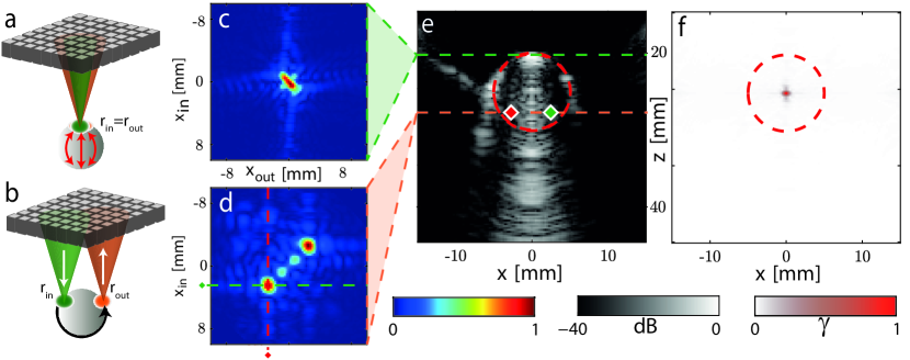
Figure 2: Elastic target signatures encoded in the reference reflection matrix. a, The reference reflection matrix $\mathbf{R}_{0}$ is measured on the target sphere placed in water. The confocal beamforming process applied to $\mathbf{R}_{0}$ selects not only the ballistic echo of the sphere but also its reverberations resulting from multiple reflections of bulk elastic waves (depicted by red arrows) at its inner surface. b, Matrix imaging decouples the input and output focal spots ³⁶, $\mathbf{r}_{\textrm{in}}$ and $\mathbf{r}_{\textrm{out}}$, to highlight the contribution of circumferential waves (depicted by a black arrow) generated by the incoming wave at a specific angle of incidence with respect to sphere surface ³². c, Cross-section of the focused reflection matrix, $\mathbf{R}_{0,xx}(y,z)$, in the plane $y=0$ and at depth $z=21$ mm showing the diagonal contribution of the ballistic echo. d, Same matrix but at depth $z=28.5$ mm showing the off-diagonal contribution of circumferential waves. e, $(x,z)$-section of the confocal image in the plane $y=0$ showing the spatio-temporal dispersion of the target echo. f, Likelihood index map ${\color[rgb]{0,0,0}\gamma}(\mathbf{r})$ (Eq. 2) built from the fingerprint operator indicating that we can accurately locate the target inside the reference environment (the sphere surface is highlighted by a red dashed line in panels e and f). Since in this case $\mathbf{R}\equiv\mathbf{R}_{0}{\color[rgb]{0,0,0}(\mathbf{r}_{0})}$, this result serves as a consistency check for the formalism.

Defining the fingerprint operator

Figure 2 thus shows that each of the two metal spheres gives rise to a scattered wave-field displaying a large number of spatio-temporal degrees-of-freedom (d.o.f). The idea is now to smartly exploit these signatures to detect and localize each target even in presence of a strong multiple scattering fog. To do so, we start from the scattering-invariant operator in reflection, $\mathbf{\Gamma}=\mathbf{R}\times{\color[rgb]{0,0,0}\mathbf{R}_{0}}^{\dagger}$, discussed above. Rather than inspecting individual eigenstates and eigenvalues of $\mathbf{\Gamma}$, however, we quantify the correlation signatures through the trace of this matrix, integrated over the entire recorded frequency interval and properly normalized:

$${\color[rgb]{0,0,0}\gamma}(\mathbf{q})=\frac{\left|\int df\textrm{Tr}\left\{{\mathbf{R}}(f)\times{\color[rgb]{0,0,0}\mathbf{R}_{0}}^{{\dagger}}(\mathbf{q},f)\right\}\right|}{\left[\int df||{\mathbf{R}}(f)||_{F}\times\int df||{\color[rgb]{0,0,0}\mathbf{R}_{0}}(\mathbf{q},f)||_{F}\right]^{1/2}},$$ (2)

where the symbol $||\cdot||_{F}$ stands for the Frobenius norm. The likelihood index ${\color[rgb]{0,0,0}\gamma}(\mathbf{q})$ for the target to be in state $\mathbf{q}$, involves an emulated target fingerprint matrix $\mathbf{R}_{0}(\mathbf{q})$, where $\mathbf{q}$ accounts for the target state such as, for instance, the target’s position $\mathbf{r}$, size, shape or any other parameter that has an influence on the target’s response.

The question relevant to the practical implementation of this approach is now the construction of the fingerprint operator. The most direct way of doing it is to consider the free space reflection matrix $\mathbf{R}_{0}(\mathbf{r}_{0})$ shown in Fig. 2 and to emulate a fingerprint matrix $\mathbf{R}_{0}({\color[rgb]{0,0,0}\mathbf{r}})$ by a virtual shift of the target from the initial position $\mathbf{r}_{0}$ to any point $\mathbf{r}$ through simple matrix operations (Methods). A first validation of Eq. 2 can be performed by applying it to the free-space reflection matrix such that $\mathbf{R}=\mathbf{R}_{0}{\color[rgb]{0,0,0}(\mathbf{r}_{0})}$. The result is displayed in Fig. 2f. The comparison with the confocal image displayed Fig. 2e highlights the benefit of the proposed approach. All the energy radiated by the elastic sphere that was initially dispersed in time and space on the diagonal and off-diagonal coefficients of the focused $\mathbf{R}-$matrix is now concentrated onto a single pixel of the image.

The gain $G$ in contrast compared to the confocal image is drastic since it scales as the product between the numbers of spatial and temporal d.o.f, $N_{S}$ and $N_{T}$, exhibited by the target (Supplementary Section S4):

$$G\sim N_{S}\times N_{T}$$ (3)

On the one hand, $N_{T}$ can be expressed as the product of the frequency bandwidth $\Delta f$ and the reverberation time $\Delta t$ of the target echo:

$$N_{T}\sim\Delta f\Delta t.$$ (4)

In the present case, the reverberation time $\Delta t$ lasts 40 $\mu$s for each sphere which yields $N_{t}\sim 32$. On the other hand, $N_{S}$ is the effective rank of the target reflection matrix $\mathbf{R}_{0}$, that can be assessed from the singular value distribution of $\mathbf{R}_{0}$ (Eq. 16, Supplementary Figure S8): $N_{S}\sim 20$ for sphere 1 and $N_{S}\sim 12$ for sphere 2. This larger value for sphere 1 is explained by an effective rank of $\mathbf{R}_{0}$ scaling as the number of lateral resolution cells covered by the target ^{15, 16}:

$$N_{S}\sim\mathcal{A}/\delta\rho_{D}^{2}$$ (5)

with $\mathcal{A}$, the target physical cross-section and $\delta\rho_{D}\sim\lambda/(2\sin\alpha)$, the diffraction-limited resolution length of the target image in Fig. 2, and $\alpha$ the angle under which the probe is seen by the array. The resolution length actually determines the transverse size of the focal spot displayed by the $\gamma-$map displayed in Fig. 2.

In the present case, given the values of $N_{S}$ and $N_{T}$ provided above, the fingerprint operator can, in principle, increase the sphere contrast by a factor $G$ (Eq. 3) ranging from 380 (sphere 2) to 640 (sphere 1). This gain is almost one order of magnitude larger than the exponential decay experienced by target echoes with respect to multiple scattering (Eq. 1). We can thus expect that the fingerprint operator shall enable detecting and localizing the spheres in the experiment of Fig. 1.

Seeing into the scattering fog

As we will show in the following, the target’s signatures can be made even more specific with respect to its environment by considering a generalized scattering invariant operator, $\hat{\mathbf{\Gamma}}=\mathbf{R}\times\mathbf{F}^{{\dagger}}$, involving a more selective fingerprint matrix ${\mathbf{F}}$ (Supplementary Section S2). To that aim, different filters are applied to the reference matrix $\mathbf{R}_{0}$ to build the matrix $\mathbf{F}$ (Methods): (i) A time filter in order to remove the specular echoes of the spheres ^{31, 32} (Eq. 13, Supplementary Figure S6); (ii) An SVD filter to whiten the signal subspace of $\mathbf{R}_{0}$ and cancelling its noise subspace (Eq. 17); (iii) An angular filter in order to account for the limited size of the ultrasonic probe (Supplementary Figure S9). This optimized fingerprint operator $\mathbf{F}$ is then used to compute the likelihood maps of the 8 mm- and 10 mm-diameter spheres in the experimental configuration. To highlight the drastic improvement provided by our approach, we superimpose the corresponding $\gamma$-maps encoded in green and red, respectively, onto the confocal image in Fig. 3, where different cross-sections of the imaged volume are displayed: While the confocal image is fully blurred by the multiple scattering fog, each likelihood map allows the unambiguous detection of each sphere. We have thus successfully demonstrated that the exponential decrease of the target echo (captured by $\mathcal{C}_{I}$ in Eq. 1) is largely compensated by the gain $G$ (Eq. 3) provided by the fingerprint operator.

Experimentally, the target contrast $\mathcal{C}_{\gamma}$ can be evaluated by considering the ratio between the value of $\gamma$ at each target position and its average outside of each target. A significant contrast ranging between 6 and 7 is found for each metal sphere (see $\mathcal{C}_{\gamma}$ values indicated for each cross-section in Fig. 3). Those values are in qualitative agreement with the theoretical prediction: $\mathcal{C}_{\gamma}\sim G\times\mathcal{C}_{I}\sim$ 4.2 for sphere 1 and 7.6 for sphere 2. This high contrast is an important feature since it can be seen as a signal-to-noise ratio that dictates the precision $\delta\rho_{L}$ of the localization process predicted by the Cramér-Rao bound ^{37, 38}: $\delta\rho_{L}\sim\delta\rho_{D}/\sqrt{\mathcal{C}_{\gamma}}$ (Supplementary Section S5). By increasing the target contrast with respect to its environment, the scattering invariant operator enhances the localization precision by a factor scaling as $\sqrt{N_{T}N_{S}}$ (Eq. 3). The more complex the target echo is, the more beneficial our method becomes.

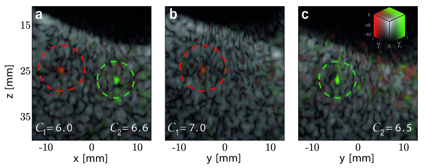
Figure 3: Detecting and localizing target metal spheres hidden in the multiple scattering fog. Different cross-sections of the $\gamma$-map for each sphere (diameter $d_{1}=10$ mm in red, $d_{2}=8$ mm in green) are superimposed to the corresponding confocal image (B&W scale in dB). a $(x,z)-$cross-section at $y=y_{1}=y_{2}$. b $(y,z)-$cross-section at $x=x_{1}$. c $(y,z)-$cross-section at $x=x_{2}$. The confocal images correspond to cross-sections of Fig. 1d, the dashed circles correspond to the known radius of each sphere. The value of the contrast $\mathcal{C}_{\gamma}$ at the target’s position with respect to the average value of $\gamma$ outside of each target is also indicated. While the targets are completely invisible in the confocal images, they appear very well localized through the calculation of their associated likelihood index $\gamma$.

To show the generality of the concept and its potential applications, a second experiment depicted in Fig. 4a (Methods) was carried out in a weaker scattering regime ($z\sim\ell_{s}$) characteristic of ultrasound imaging and in which single and multiple scattering coexist ³⁰. It involves the detection of a lesion marker (Tumark®Vision, Somatex, Fig. 4b) generally used to monitor breast tumors in clinical settings ³⁹. Although these markers have been specifically designed to yield a clear signature on ultrasound images, their detection and localization are often hampered by the ultrasound speckle generated by unresolved scatterers that are randomly distributed in tissue. In the experiment depicted in Fig. 4, ultrasound speckle is generated by a foam soaked in water in which the lesion marker has been embedded. This foam generates an ultrasound speckle similar to that of soft tissues. The corresponding confocal image highlights this characteristic speckle which here prevents an unambiguous detection and localization of the target (Fig. 4c). On the contrary, the fingerprint operator designed for this lesion marker allows a clear detection and sharp localization of the lesion marker (Fig. 4d). This proof-of-concept shows the potential of the fingerprint operator for the monitoring of any object (e.g. needle, catheter, marker, etc.) used in interventional radiology.

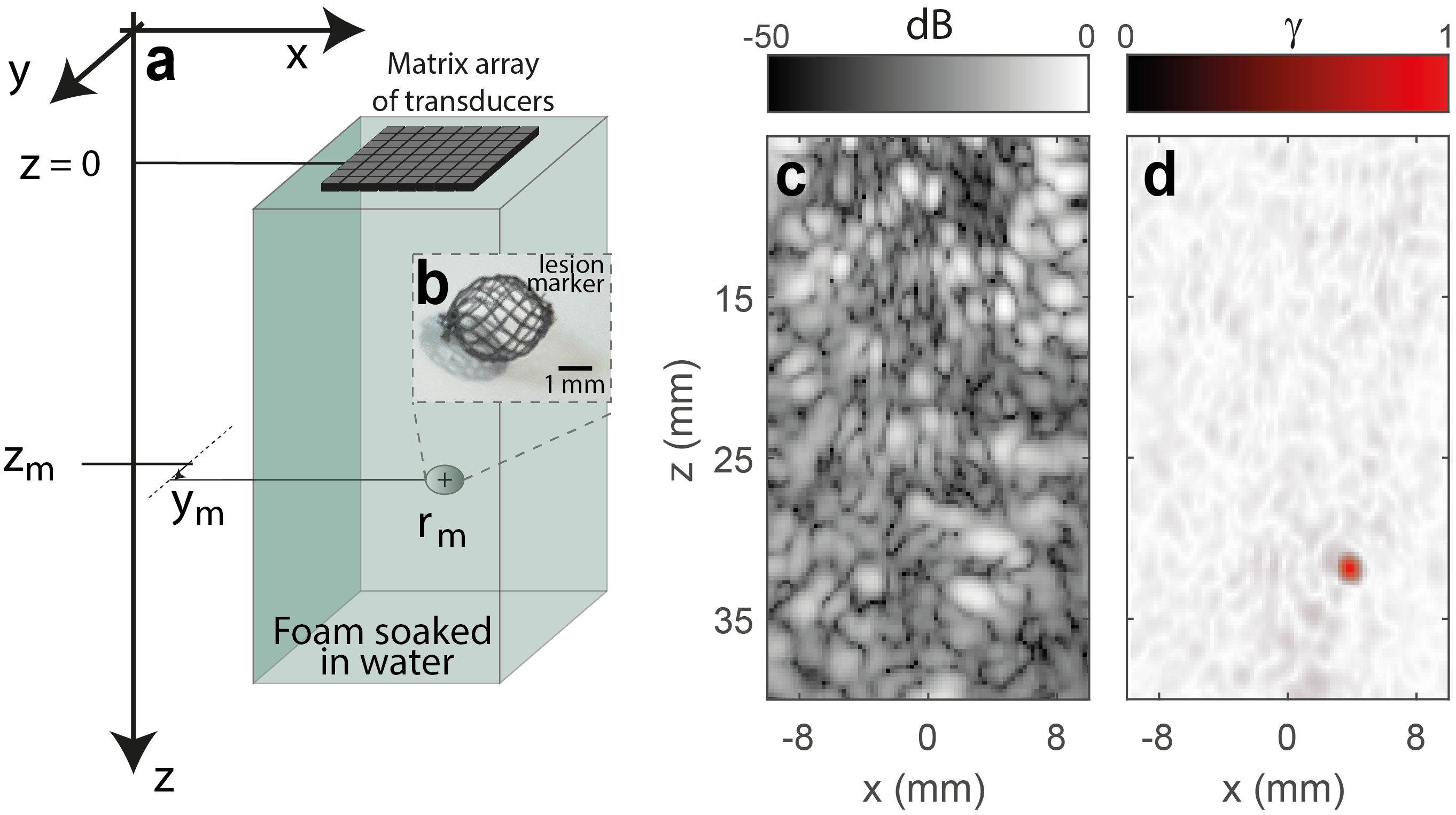
Figure 4: Localizing a lesion marker in ultrasound speckle. a, Experimental configuration: The $32\times 32$ probe is used to image a lesion marker embedded into foam soaked in water. The position $\mathbf{r}_{m}=(x_{m},y_{m},z_{m})$ of the lesion marker center is $(3.5,4.5,32)$ mm. b, Photography of the lesion marker (credit: Arthur Le Ber). c, Longitudinal cross-section of the confocal ultrasound image in the plane $y=y_{m}$. d, Corresponding likelihood map of the lesion marker superimposed onto the confocal image in transparency.

Towards quantitative imaging of complex media

Beyond the detection and localization of an intruder inside a complex medium, the fingerprint operator can also be leveraged for a quantitative characterization of the medium itself. In particular, we will show how it can be used for mapping the local anistropy of a fibrous medium by applying our approach to muscle tissue (Fig. 5b). This information is particularly relevant in ultrasound imaging for diagnosing neuromuscular ⁴⁰ or myocardial ⁴¹ diseases.

The experiment is carried out on a human calf, in-vivo, the fibers of which are partially visible on the ultrasound image displayed in Fig. 5b. This image is built from the reflection matrix $\mathbf{R}$ recorded using a linear phased array of 256 transducers over the [5.5; 9.5] MHz frequency bandwidth (Methods). In order to image fibrous tissues, the fingerprint matrix is defined as a free-space reflection matrix $\mathbf{R}_{0}(\mathbf{q})$ associated with a reflecting mirror whose state $\mathbf{q}$ is described by its position $\mathbf{r}$, its orientation $\alpha$ and its dimension $L$ (Fig. 5a). The dictionary of fingerprint matrices $\mathbf{R}_{0}(\mathbf{q})$ is constructed numerically (Methods).

The scalar product of the recorded reflection matrix $\mathbf{R}$ with the fingerprint matrix $\mathbf{R}_{0}$ (Eq. 2) provides a likelihood index ${\color[rgb]{0,0,0}\gamma}(\mathbf{r},\alpha,L)$ with respect to the parameters $\alpha$ and $L$ at each point $\mathbf{r}$ in the image (Eq. 2). The dependence of the ${\color[rgb]{0,0,0}\gamma}$-map with respect to parameters $\alpha$ and $L$ is shown for two points $\mathbf{r}$ in the field-of-view in Figs. 5c and d. The maximum value of this quantity gives the orientation $\alpha_{\textrm{opt}}(\mathbf{r})$ and the local correlation length $L_{\textrm{opt}}(\mathbf{r})$ of the fibrous medium at each point $\mathbf{r}$:

$$\{\alpha_{\textrm{opt}}(\mathbf{r}),L_{\textrm{opt}}(\mathbf{r})\}=\arg\max_{\{\alpha,L\}}\left[\gamma(\mathbf{r},\alpha,L)\right]$$ (6)

The size and orientation distribution of the fibers provide a vector representation of the fibers superimposed to the confocal image in Fig. 5e. A very good agreement is found between the visual appearance of the fibers on the ultrasound image and their vector representation provided by the fingerprint operator.

Note that this approach is a generalization of the specular beamforming procedure developed in a previous study ⁴². In the language of the fingerprint operator, an infinite mirror was considered as the reference object and its orientation was the free parameter. While this method was relevant for revealing the presence of large objects such as needles with ultrasound, the simultaneous determination of the correlation length $L_{\textrm{opt}}$ and fiber orientation $\alpha_{\textrm{opt}}$ is required to retrieve the complex architecture of fibers. Compared to alternative approaches relying on spatial correlations of the reflected wave-field that only determine the orientation of fibers in a plane parallel to the probe ⁴¹, the current approach can provide the 3D orientation of fibers with a 2D array of transducers. This information could be extremely rewarding to monitor neuro-muscular diseases ⁴⁰ and myocardial fiber disarray that emerges in the early stage of many pathologies such as in cardiomyopathies or in fibrosis ⁴³. It can also be relevant in the context of non-destructive testing for determining the orientation of elongated grains in polycrystalline materials ⁴⁴. In optical microscopy, collagen fibrils are the major mechanical component in the extracellular matrix of biological tissues ⁴⁵. While second harmonic generation has proved to be a unique tool for probing ex-vivo the collagen orientation and its lamellar distribution in cornea ⁴⁶, the proposed matrix method can be an interesting alternative for in-vivo applications ⁴⁷.

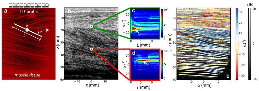
Figure 5: Revealing the local architecture of fibers in muscle tissue. a, Sketch of the experimental configuration: An array of transducers is placed in contact with the calf of a healthy patient. The fingerprint operator $\mathbf{R}_{0}(\mathbf{q})$ here corresponds to a set of reflection matrices associated with a mirror of size $L$ and orientation $\alpha$ simulated for each pixel $\mathbf{r}$ in the medium considered as homogeneous ($c_{0}=$ 1580 m/s). b, Ultrasound image of the calf in dB. c, d, Likelihood index $\gamma$ in the $(L,\alpha)$ parameter space for two positions yielding different values for the local correlation length $L$ and fiber orientation $\alpha$. The white arrows indicate the optimal length $L_{\textrm{opt}}$ and orientation $\alpha_{\textrm{opt}}$ at each position. e, Vector representation of the fibers deduced from the orientation distribution $\alpha_{\textrm{opt}}(\mathbf{r})$ encoded with the color scale displayed on the right.

Discussion

In this manuscript, we have introduced the fingerprint operator with the aim to detect, localize and characterize any object in a strongly scattering medium. A necessary condition, however, is the creation of a sufficiently complete and precise knowledge of the reflection matrix and its dependence according to a state of interest. From that perspective, the generalized polarization tensor, that was introduced ten years ago for electromagnetic waves, can be of interest ^{48, 49}. The generalized polarization tensor can be obtained from the $\mathbf{R}$-matrix by solving a set of linear equations. Ammari et al.  ^{48, 49} have conceived an algorithm to identify a target from a dictionary of generalized polarization tensors. The position and shape of the target are then obtained from one element of the dictionary after a given rotation, size scaling and translation. Unfortunately, this approach requires an array of sensors fully surrounding the target under investigation, which is not available in most in-vivo or in-situ applications. On the contrary, the fingerprint operator works in reflection and can be adapted to any experimental configuration, thereby providing much higher robustness with respect to the non-ideal nature of experiments.

Beyond target localization and identification, the fingerprint operator is extremely promising for characterizing objects whose spatio-temporal response depends on their environment, thereby allowing a local measurement of intensive physical quantities, such as temperature or pressure. In ultrasound imaging, microbubbles are ideal candidates for this purpose. They are widely used as contrast agents and they exhibit a complex resonance spectrum that strongly depends on their environment ⁵⁰, in particular on the local pressure ⁵¹. Coupled to ultrasound localization microscopy  ⁵², where microbubbles are tracked to perform super-resolved imaging of the vascular network, our approach could be used to map the local pressure inside the brain vessels. Such an observable would be an extremely useful information for stroke diagnosis ⁵³.

We envision that the accessible depth-range of our approach can be further increased by incorporating any available a-priori knowledge on the target’s environment, such as its heterogeneity. On the other hand, the fingerprint matrix $\mathbf{F}$ could also be used in conjunction with the distortion matrix concept ^{21, 22}. Any complex object could then be used as a virtual point-like guide star (Fig. 2f) in a computational adaptive focusing scheme ²³.

Beyond its versatility, the fingerprint operator is also a universal concept that can find applications in all fields of wave physics where multi-element technology is available. MIMO radar ⁵⁴ and sonar ⁵⁵ are examples of fields where target identification and localization in noisy environments is a long-lasting challenge. At a much smaller scale, cells exhibit a complex optical response that strongly depends on their shape ⁵⁶, refractive index distribution ⁵⁷ and applied stress ⁵⁸. The fingerprint operator therefore constitutes an adequate tool to probe these intrinsic parameters and to monitor cell development in 3D whether it be for embryology ⁵⁹ or pharmacology thanks to the fast development of organoids ⁶⁰. While this is by no means an exhaustive list, the flexibility of the fingerprint operator concept can be critical to all of these applications.

Methods

Ultrasound scanners and probes.

In the elastic sphere and lesion marker experiments, the acquisition of the reflection matrix is performed using a 2D matrix array of transducers (Vermon) whose characteristics are provided in Tab. 1. The electronic hardware used to drive the probe was developed by Supersonic Imagine in the context of a collaboration agreement with the Langevin Institute.

In the calf experiment, the acquisition is performed using a medical ultrafast ultrasound scanner (Aixplorer Mach-30, Supersonic Imagine, Aix-en-Provence, France). The skin is placed in direct contact of a linear array of transducers (SL15-4, Supersonic Imagine) whose characteristics are also provided in Tab. 1.

Experiments	Elastic sphere	Muscle tissue
	Lesion marker
Probe	2D array	1D array
Number of transducers	$32\times 32$	256
Inter-element distance $\delta u$	$0.5$ mm	0.2 mm
Transducer directivity $\theta_{d}$	$28^{\circ}$	$35^{\circ}$
Maximum Angle $\theta_{m}$	$28^{\circ}$	$25^{\circ}$
Angular Pitch $\delta\theta$	$0.8^{\circ}$	$0.5^{\circ}$
Number of plane waves $N_{\theta}$	$1225$	$101$
Central frequency $f_{c}$	$2.2$ MHz	7.5 MHz
Bandwidth (at $-6$dB)	1.8-2.6 MHz	5.5-9.5 MHz
Sampling frequency $f_{s}$	6 MHz (IQ)	30 MHz

Table 1: Experimental parameters.

Acquisition of the reflection matrix.

In each case, the reflection matrix is acquired using a set of plane waves ⁶¹. For each plane wave of angles of incidence $\bm{\theta}_{\textrm{in}}=(\theta_{x},\theta_{y})$, the time-dependent reflected wave field $R(\mathbf{u}_{\textrm{out}},\bm{\theta}_{\textrm{in}},t)$ is recorded by each transducer $\mathbf{u}_{\textrm{out}}$. This set of wave-fields forms a reflection matrix acquired in the plane wave basis, $\mathbf{R}_{\mathbf{u}\bm{\theta}}(t)=\left[R(\mathbf{u}_{\textrm{out}},\bm{\theta}_{\textrm{in}},t)\right]$. Since the transducer and plane wave bases can be related by a simple Fourier transform at the central frequency, the array pitch $\delta u$ and probe size $\Delta u$ dictate the angular pitch $\delta\theta$ and maximum angle $\theta_{max}$ necessary to acquire a full reflection matrix in the plane wave basis (Tab. 1). A set of plane waves are thus generated by applying appropriate time delays $\Delta\tau(\bm{\theta}_{\textrm{in}},\mathbf{u}_{\textrm{in}})$ to each transducer $\mathbf{u}_{\textrm{in}}=(u_{x},u_{y})$ of the probe:

$${\Delta\tau(\bm{\theta}_{\textrm{in}},\mathbf{u}_{\textrm{in}})}=[u_{x}\sin\theta_{x}+u_{y}\sin\theta_{y}]/{c_{0}}.$$ (7)

where $c_{0}$ is the assumed speed-of-sound. The angular pitch and range as well as the number of illuminations are reported for each experiment in Tab. 1.

Focused beamforming of the reflection matrix.

To form an image from the measured reflection matrix, a beamforming procedure has to be applied in emission and reception in order to generate a synthetic focusing on each focal point. In the time domain, a delay-and-sum beamforming process can be performed by applying appropriate time delays to the recorded signals ²³. In the frequency domain, matrix products can be applied to project $\mathbf{R}$ in the focused basis. The projection of the $\mathbf{R}-$matrix in the focused basis can be performed at each depth $z$ by means of the following matrix product:

$${\mathbf{R}}_{\bm{\rho\rho}}(z,f)=\mathbf{G}_{\mathbf{u}\bm{\rho}}^{\dagger}(z,f)\times{\mathbf{R}}_{\mathbf{u}\boldsymbol{\theta}}(f)\times\mathbf{P}_{\boldsymbol{\theta}\bm{\rho}}^{*}(z,f).$$ (8)

where $\mathbf{P}_{\boldsymbol{\theta}\bm{\rho}}(z,f)=\left[P\left(\boldsymbol{\theta},\bm{\rho},z,f\right)\right]$ and $\mathbf{G}_{\mathbf{u}\bm{\rho}}(z,f)=\left[G\left(\mathbf{u},\bm{\rho},z,f\right)\right]$ are the free space propagation matrices from the focused basis ($\bm{\rho}$) at depth $z$ to the plane wave ($\bm{\theta}$) and transducer ($\mathbf{u}$) bases, respectively. Assuming an homogeneous speed of sound $c_{0}$, the coefficients of $\mathbf{P}_{\boldsymbol{\theta}\bm{\rho}}$ are expressed as follows

$$P(\boldsymbol{\theta},\bm{\rho},f)=\exp\left[ik\left(x\sin\theta_{x}+y\sin\theta_{y}+z\sqrt{1-\sin^{2}\theta_{x}-\sin^{2}\theta_{y}}\right)\right].$$ (9)

with $k=2\pi f/c_{0}$, the wave number. The coefficients of $\mathbf{G}_{\mathbf{u}\bm{\rho}}(z,f)$ are the 2D or 3D Green’s function of the wave equation in homogeneous media:

$${G}_{2D}(\mathbf{u},\bm{\rho},z,f) =\frac{-i}{4}\mathcal{H}^{(1)}_{0}\left(k\sqrt{||\bm{\rho}-\mathbf{u}||^{2}+z^{2}}\right),$$ (10a)

$${G}_{3D}(\mathbf{u},\bm{\rho},z,f) =-\frac{\exp\left(ik\sqrt{||\bm{\rho}-\mathbf{u}||^{2}+z^{2}}\right)}{4\pi\sqrt{||\bm{\rho}-\mathbf{u}||^{2}+z^{2}}}.$$ (10b)

where $\mathcal{H}^{(1)}_{0}$ is the Hankel function of the first kind. Each coefficient of ${\mathbf{R}}_{\bm{\rho\rho}}(f)=[{R}(\bm{\rho}_{\textrm{out}},\bm{\rho}_{\textrm{in}},f)]$ is the response between a virtual source at point $(\bm{\rho}_{\textrm{in}},z)$ and a virtual detector at $(\bm{\rho}_{\textrm{out}},z)$ at frequency $f$ [Fig. 2e].

In order to retrieve the axial resolution provided by the broadband feature of ultrasonic signals, a broadband focused reflection matrix $\overline{\mathbf{R}}_{\bm{\rho\rho}}(z)$ can be derived at each depth by coherently summing the monochromatic matrices over the frequency bandwidth:

$$\overline{\mathbf{R}}_{\bm{\rho\rho}}(z)=\frac{1}{\Delta f}\int^{f_{+}}_{f_{-}}df{\mathbf{R}}_{\bm{\rho\rho}}(z,f),$$ (11)

where $f_{\pm}=f_{c}\pm\Delta f/2$ and $f_{c}$ is the central frequency. Each element of ${\mathbf{R}}_{\bm{\rho\rho}}(z)$ contains the signal that would be recorded by a virtual transducer located at $({\color[rgb]{0,0,0}\bm{\mathrm{\rho}}_{\mathrm{out}}},z)$ just after a virtual source at $({\color[rgb]{0,0,0}\bm{\mathrm{\rho}}_{\mathrm{in}}},z)$ emits a pulse of length $\delta t=\Delta f^{-1}$ at the central frequency $f_{c}$. Cross-sections $\overline{\mathbf{R}}_{xx}(y,z)$ of the focused reflection matrix are displayed for the free space sphere experiment in the mid-plane $y=0$ and at depths $z=21$ mm and 28.5 mm in Figs. 2c and d, respectively. A time-gated confocal image $\mathcal{I}(\bm{\rho},z)$ can be extracted from the diagonal of the broadband focused $\mathbf{R}-$matrix, such that:

$$\mathcal{I}(\bm{\rho},z)=\left|\overline{R}(\bm{\rho},\bm{\rho},z)\right|^{2}.$$ (12)

The resulting confocal images are displayed in Figs. 1d, 2e, 3, 4c and 5b for the different experiments described in the paper.

Fingerprint operator based on a calibration measurement

To build the fingerprint operator, the first strategy is to start from the measurement of a free-space reflection matrix $\mathbf{R}_{0}$ associated with the target at a given position $\mathbf{r}_{0}$. In principle, this matrix can be used as the value of the fingerprint operator at position $\mathbf{r}_{0}$: $\mathbf{F}(\mathbf{r}_{0})\equiv\mathbf{R}_{0}$. In that case, the operation described in Eq.  2 can be seen as an adaptive filter. This kind of filter may be not the most adequate approach for detection and localization purposes.

First, depending on the experimental configuration, this reference matrix might be not necessarily specific enough with respect to the target environment (Supplementary Figure S5). In the sphere localization experiment, the ballistic echo of each sphere shall be removed in order for the fingerprint matrix not to be dominated by the strong specular echo generated by the interface of the granular medium in the original experiment (Fig. 1d). To that aim, the reference matrix $\mathbf{R}_{0}$ is filtered in the time domain by means of a Heavyside filter (Supplementary Figure S6), such that:

$${R}^{\prime}_{0}(\mathbf{u}_{\textrm{out}},\bm{\theta}_{\textrm{in}},t)={R}_{0}(\mathbf{u}_{\textrm{out}},\bm{\theta}_{\textrm{in}},t)H(t-\tau_{\textrm{in}}(\bm{\theta}_{\textrm{in}},\mathbf{r}_{0})-\tau_{\textrm{out}}(\mathbf{u}_{\textrm{out}},\mathbf{r}_{0})-\delta t)$$ (13)

with $\delta t\sim 1/\Delta f$, the temporal resolution of the recorded signals. $\tau_{\textrm{in}}$ and $\tau_{\textrm{out}}$ are the expected times-of-flight for the ballistic wave from the probe to the cylinder surface. At output (transducer basis), the time-of-flight $\tau_{\textrm{out}}$ can be expressed as follows:

$$\tau_{\textrm{out}}(\mathbf{u},\mathbf{r}_{0})=\frac{\sqrt{(x_{0}-u_{x})^{2}+(y_{0}-u_{y})^{2}+(z_{0}-d/2)^{2}}}{c_{0}}.$$ (14)

At input (plane wave basis), $\tau_{\textrm{in}}$ is given by

$${\tau_{\textrm{in}}(\bm{\theta},\mathbf{r}_{0})}=\left[x_{0}\sin\theta_{x}+y_{0}\sin\theta_{y}+(z_{0}-d/2)\sqrt{1-\sin^{2}\theta_{x}-\sin^{2}\theta_{y}}\right]/{c_{0}}.$$ (15)

Second, the transfer function of an adaptive filter is not flat. Both the temporal and spatial frequency spectrum of the target can thus be altered if we consider $\mathbf{F}(\mathbf{r}_{0})\equiv\mathbf{R}_{0}$ in Eq. 2. This would reduce both the axial and transverse resolution of the imaging method in the real space and decrease the contrast of the target in the $\gamma$-map of the target likelihood index. To optimize the target signal, an inverse filter could be applied by considering the inverse matrix of $\mathbf{R}^{\prime}_{0}$ as the building block of the fingerprint operator $F(\mathbf{r}_{0})$. However, this would be at the price of an extreme sensitivity with respect to experimental noise and a loss in terms of signal-to-noise ratio.

A good compromise between an adaptive and inverse filtering process can be reached by performing a spectral whitening of $\mathbf{R}^{\prime}_{0}$. In practice, this can be done by performing the singular value decomposition of ${\mathbf{R}}^{\prime}_{0}(f)$ at each frequency $f$ (Supplementary Figure S8):

$${\mathbf{R}}^{\prime}_{0}(f)=\sum_{p}\sigma_{p}(f)\mathbf{U}_{p}(f)\mathbf{V}_{p}^{{\dagger}}(f)$$ (16)

where $\mathbf{U}_{p}$ and $\mathbf{V}_{p}$ are the output and input singular vectors of $\mathbf{R}^{\prime}_{0}$. While, for a point-like target, the reflection matrix would only exhibit a predominant singular value, the spectrum of ${\mathbf{R}}^{\prime}_{0}(f)$ displays a continuum of singular values due to the target size and the different resonant modes supported by each sphere (Supplementary Section S3).

To ensure the robustness of Eq. 2 with respect to experimental noise, only the eigenstates associated with the largest singular values shall be kept. In pratice, the rank $N_{S}$ of the fingerprint operator is arbitrarily chosen such that the singular value ratio $\sigma_{i}/\sigma_{1}$ is larger than 0.4 (Supplementary Figure S8). The fingerprint operator is then obtained by whitening the singular value spectrum of this signal subspace such that:

$$\mathbf{F}(\mathbf{r}_{0},f)=\sum_{p=1}^{N_{S}}\mathbf{U}_{p}(f)\mathbf{V}_{p}^{{\dagger}}(f)$$ (17)

Virtual shift of the target

The next step is to deduce the spatial evolution of the fingerprint operator from its value at $\mathbf{r}_{0}$. This is done by performing a virtual translation of the target on each point $\mathbf{r}$ of the field-of-view. To that aim, the fingerprint matrix shall be projected at output in the plane wave basis:

$${\mathbf{F}}_{\bm{\theta}\bm{\theta}}(\mathbf{r}_{0},f)=\mathbf{P}_{\mathbf{\theta}\mathbf{u}}(f)\times{\mathbf{F}}_{\mathbf{u}\mathbf{\theta}}(\mathbf{r}_{0},f)$$ (18)

From the plane wave basis, the target can be virtually shifted to any position $\mathbf{r}=\mathbf{r}_{0}+\Delta\mathbf{r}$ by the application of a shift operator $\mathbf{S}(\Delta\mathbf{r})$ at input and output of the matrix $\mathbf{F}_{\bm{\theta}\bm{\theta}}(\mathbf{r}_{0},f)$. Mathematically, it can be written as the following matrix product:

$${\mathbf{F}}_{\bm{\theta}\bm{\theta}}(\mathbf{r},f)=\mathbf{S}(\Delta\mathbf{r},f)\circ{\mathbf{F}}_{\bm{\theta}\bm{\theta}}(\mathbf{r}_{0},f)\circ\mathbf{S}(\Delta\mathbf{r},f)$$ (19)

where the symbol $\circ$ stands for the Hadamard (element wise) product. In terms of matrix coefficients, the previous equation writes

$${{F}}(\bm{\theta}_{\textrm{out}},\bm{\theta}_{\textrm{in}},\mathbf{r},f)={S}(\bm{\theta}_{\textrm{out}},\Delta\mathbf{r},f){{F}}(\bm{\theta}_{\textrm{out}},\bm{\theta}_{\textrm{in}},\mathbf{r}_{0},f){S}(\bm{\theta}_{\textrm{in}},\Delta\mathbf{r},f)$$ (20)

where the coefficients $S(\bm{\theta},\Delta\mathbf{r},f)$ of the shift operator $\mathbf{S}(\Delta\mathbf{r},f)$ write

$$S(\bm{\theta},\Delta\mathbf{r},f)=A(\bm{\theta},\mathbf{r})P(\bm{\theta},\mathbf{r},f)P^{*}(\bm{\theta},\mathbf{r}_{0},f)=A(\bm{\theta},\mathbf{r})P(\bm{\theta},\Delta\mathbf{r},f)$$ (21)

where $A(\bm{\theta},\mathbf{r})$ is an apodization factor that limits the angular range of the synthetic aperture at emission and reception which depends on whether the plane wave can reach the target at point $\mathbf{r}$ or not (Supplementary Figure S9).

At last, the fingerprint operator can be projected back onto the acquisition basis of the recorded reflection matrix $\mathbf{R}$, such that

$${\color[rgb]{0,0,0}\mathbf{F}}_{\mathbf{u}\bm{\theta}}(\mathbf{r},f)=\mathbf{P}_{\mathbf{\theta}\mathbf{u}}^{{\dagger}}(f)\times{\color[rgb]{0,0,0}\mathbf{F}}_{\bm{\theta}\bm{\theta}}(\mathbf{r},f)$$ (22)

Numerical computation of the fingerprint operator

In the calf experiment, the fingerprint operator corresponds to a set of reflection matrices associated with a plane mirror of constant reflectivity characterized by a state $\mathbf{q}$ accounting for its position $\mathbf{r}$, orientation $\alpha$ and characteristic size $L$: $\mathbf{q}=\left\{\mathbf{r},\alpha,L\right\}$. (cf Fig. 5a). Each reference matrix $\mathbf{R}_{\mathbf{u}\bm{\theta}}(\mathbf{q},f)$ is computed numerically using the following matrix product:

$${\mathbf{R}}_{0}(\mathbf{q})=\mathbf{G}_{\mathbf{u}\mathbf{r}}(f)\times\boldsymbol{\Gamma}_{\mathbf{r}\mathbf{r}}(\mathbf{q})\times\mathbf{G}_{\mathbf{u}\mathbf{r}}^{\top}(f)\times\mathbf{P}_{\boldsymbol{\theta}\mathbf{u}}^{\dagger}(f),$$ (23)

where $\boldsymbol{\Gamma}_{\mathbf{r}\mathbf{r}}(\mathbf{q})$ is a diagonal matrix whose diagonal coefficients $\gamma(\mathbf{r})$ stand for the reflectivity of the mirror in state $\mathbf{q}$. Note that, for such an object, the rank of the reflection matrix is equal to the number of resolution cells within the object, and that the $N_{S}$ non-zero singular values are degenerate ¹⁶. The adaptive filter [${\color[rgb]{0,0,0}\mathbf{F}}(\mathbf{q})=\overline{{\color[rgb]{0,0,0}R}}_{0}(\mathbf{q})$] or inverse filter operation [${\color[rgb]{0,0,0}\mathbf{F}}(\mathbf{q})={\color[rgb]{0,0,0}\mathbf{R}}_{0}^{-1}(\mathbf{q})$] are therefore equivalent in this specific case.

Data availability. The ultrasound data generated in this study are available at Zenodo ⁶² (https://zenodo.org/records/14845780).

Acknowledgments. The authors wish to thank the Somatex Company for providing the lesion marker. The authors are grateful for the funding provided by the European Research Council (ERC) under the European Union’s Horizon 2020 research and innovation program (grant agreement no. 819261, REMINISCENCE project, A.A.). This project has also received funding from Labex WIFI (Laboratory of Excellence within the French Program Investments for the Future; ANR-10-LABX-24 and ANR-10-IDEX-0001-02 PSL*, M.F.). L.M.R. was supported by the Austrian Science Fund (FWF) through Project no. P32300-N27 (WaveLand).

Author Contributions Statement. A.A. and S.R. initiated the project. A.A. supervised the project. A.L.B. and X.J. designed and performed the experiments on the granular medium. A.L.B. performed the experiment on the lesion marker experiment. A.L.B. developed the post-processing tools for the target detection experiment. W.L. performed the muscle tissue experiment. A.G. developed the post-processing tools for the muscle tissue experiment. A.L.B., A.G., L.M.R., S.R. and A.A. developed the concept of the fingerprint operator and performed the theoretical study. A.L.B. and A.G. prepared the figures. A.L.B., A.G. and A.A. prepared the manuscript. A.L.B., A.G., L.M.R., W.L., X.J., M.F., A.T., S.R. and A.A. discussed the results and contributed to finalizing the manuscript.

Competing interests. A.L.B., A.G., L.M.R., W.L., X.J., M.F., A.T., S.R. and A.A. are inventors on a french patent related to this work held by Supersonic Imagine and CNRS (no. FR2314789, filed December 2023). M.F. is cofounder of the SuperSonic Imagine company, which is commercializing one of the ultrasound platforms used in this study. W.L. is an employee of this company.

Supplementary Material

S1 Characterization of the dense granular suspension

To measure the extinction length of the ballistic or direct wave, a transmission configuration can be considered ⁶³(Fig. S1). Two transducers (Olympus, model V382-SU ) are used to measure the coherent wave across the medium (circular aperture, diameter 12.7 mm, central frequency 3.5 MHz, bandwidth at -6 dB of the order of 70%). One is working as a source and emits a quasi incident plane wave :

$$\psi_{\textrm{inc}}(t)=\psi_{0}\cos(2\pi f_{c}t)\exp\left[-{t^{2}}/(2\sigma^{2})\right]$$ (S1)

with $f_{c}=3$ MHz and $\sigma=1/(2f_{c})$. The other transducer is used a receiver. The two transducers are mounted opposite each other along a common central axis. The use of a wide transducer at reception is justified by the nature of the transmitted wave-field $\psi$ that is made of a coherent component $\left\langle\psi\right\rangle$ that resists to averaging over disorder and a multiple scattering coda $\delta\psi(\bm{\rho},z,t)$ wave that should vanish upon averaging over a number of independent disorder configurations ($\bm{\rho}$ here accounts for the lateral position with respect to the $z-$axis). Taking advantage of spatial ergodicity, the coherent wave-field can be estimated by averaging the transmitted wave-field: (i) over the transducer area; (i) on different acquisitions separated by a mixing phase of the granular medium. The multiple scattering “coda” forms a speckle pattern with each grain having an area comparable to the squared wavelength. Consequently, by choosing a circular transducer for reception whose active surface is 12.7 mm in diameter, the acquired signal is therefore averaged over around 500 speckle grains at 3 MHz which gives a reliable estimator of the coherent wave.

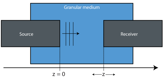
Figure S1: Measuring the scattering mean free path $\ell_{s}$ in the granular material. Experimental set up dedicated to the measurement of the coherent wave across the granular medium. An acoustic wave generated by a transducer disk propagates through the medium and is recorded by a similar transducer disk centered on the first one and placed at a distance $z$ from it.

The receiver is mounted on a translation stage, which makes it possible to automate the measurement of the coherent wave for many distances $z$. In practice, we chose to vary $z$ from a few millimetres to around 40 mm, in steps of 0.1 mm, corresponding to almost 400 measurement points. To reduce electronic noise, the signals transmitted after many 2048 successive wave trains have been summed. A spatio-temporal window is then applied to the ultrasound data, so as to eliminate the multiple reflections between the transducers. A Fourier transform is finally performed in order to extract the Fourier-dependence of the coherent wave $\left\langle\psi\right\rangle(z,f)$.

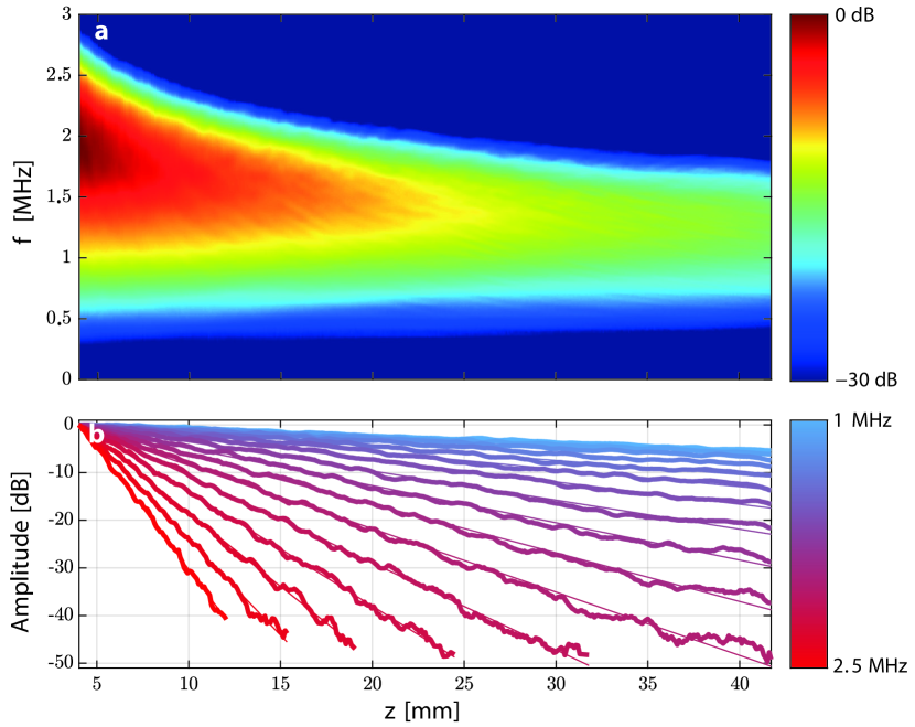
Figure S2: Depth evolution of the frequency spectrum of the coherent wave $\langle\psi(z,f)\rangle$. a, Depth-frequency dependence of $\left|\langle\psi(z,f)\rangle\right|$. b, Depth dependence of $\left|\langle\psi(z,f)\rangle\right|$ normalized by its value at $z=0$ at each frequency. The result is shown for a set of frequencies whose values are encoded with the color scale displayed on the right of the panel.

Theoretically, the coherent wave-field can be expressed as follows:

$$\left\langle\psi\right\rangle(z,f)=\psi_{0}(f)\exp\left(\frac{i2\pi f}{c_{\phi}(f)}z-\frac{z}{2\ell_{\textrm{ext}}(f)}\right)$$ (S2)

with $c_{\phi}$, the phase velocity and

$$\ell_{\textrm{ext}}=\left[\ell_{s}^{-1}+\ell_{a}^{-1}\right]^{-1},$$ (S3)

the extinction length, taking into account both the scattering losses characterized by a scattering mean free path $\ell_{s}$ and absorption losses quantified by a characteristic absorption length $\ell_{a}$. A measurement of $\ell_{\textrm{ext}}$ is then performed at each frequency $f$ by investigating the depth decay of $\left|\left\langle\psi\right\rangle(z,f)\right|$ (Fig. S2a). A linear fitting of $\ln\left(\left|\left\langle\psi\right\rangle(z,f)\right|\right)$ provides a measurement of $\ell_{\textrm{ext}}$ at each frequency (Fig. S2b).

The result is displayed in Fig. S3. In the low frequency regime ($k_{0}a\ll 1$), the value of $\ell_{\textrm{ext}}$ follows a Rayleigh scattering law and is therefore extremely dispersive. At frequency $f=2.2$ MHz, the extinction length is $\ell_{\textrm{ext}}\simeq 1.5$ mm (black arrow in Fig. S3).

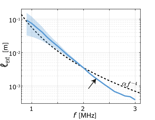
Figure S3: Measurement of the extinction length in granular media. The measured extinction length $\ell_{\textrm{ext}}$ (blue line) is compared to the Rayleigh prediction (black dashed line). The black arrow indicates the scattering condition of the experiment depicted in Fig. 1

The wave velocity $c_{\phi}$ has also been measured by investigating the phase of the coherent wave ⁶⁴. A value close to the speed-of-sound $c_{0}$ in water is found at the central frequency $f_{c}=2.2$ MHz: $c_{\phi}(f_{c})\simeq c_{0}=1.55$ mm/$\mu$s.

At last, the temporal dependence of the ensemble average transmitted intensity ^{65, 66} has also been investigated to measure transport parameters in the granular medium in a higher frequency regime. Interestingly, such measurements provide a measurement of the absorption length $\ell_{a}\simeq 8$ mm ⁶⁴ that we assume here as independent on frequency. Injecting the values measured for $\ell_{a}$ and $\ell_{\textrm{ext}}$ into Eq. S3 has led to the following estimation for the scattering mean free path: $\ell_{s}\simeq 1.8$ mm at the central frequency $f_{c}=2.2$ MHz.

S2 Free-space reflection matrix

The experimental set-up used to record the free-space reflection matrix (Fig. 2) associated with each sphere is displayed in Fig. S4. The sphere is immersed in water and attached by two sewing threads glued on his surface. These threads can actually be seen in the ultrasound image shown in Fig. 2e.

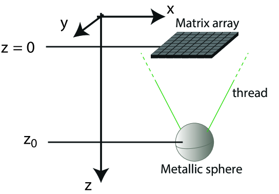
Figure S4: Experimental set up used to record the free space reflection matrix of the metallic sphere.

Figure S5 shows the likelihood index map for sphere 1 using the raw matrix $\mathbf{R}_{0}$ as the fingerprint operator ($\mathbf{F}=\mathbf{R}_{0}$). This operator completely fails to reveal the presence of sphere 1 because the direct echo of the sphere is not specific with respect to its environment. The interface of the scattering medium actually generates a strong specular echo that accounts for the surintensity of the $\gamma-$map lying along the dashed white line in Fig. S5a. There is a vertical shift of 5 mm with respect to the real position of the interface in the confocal image that corresponds to the radius of sphere 1.

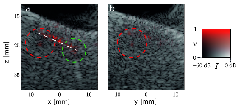
Figure S5: Detrimental effect of specular echoes on the likelihood index map. Confocal image (B&W scale) and superimposed $\gamma$-map (red scale) associated with the 10-mm diameter sphere. The $\gamma$-map is built using the raw matrix $\mathbf{R}_{0}$ as the fingerprint operator. The frequency bandwidth is 1.5-2.5 MHz. a, $(x,z)-$ cross-section in the plane $y=y_{1}$. The white dashed line shows the artifact due the specular echoes on the granular medium surface. b, $(x,z)-$ cross-section in the plane $x=x_{1}$. The positions of spheres 1 and 2 are represented by red and green dashed lines, respectively.

As described in the Methods section, a time filtering of specular echoes should thus be performed on each free-space reflection matrix (Eq. 13), in order to make the fingerprint operator more specific. Figure S6 illustrates the effect of this filter: (i) on the raw signals by comparing the initial dataset before (Fig. S6a) and after (Fig. S6b) filtering of the specular sphere echo; (ii) on the confocal image extracted from the measured (Fig. S6c) and filtered (Fig. S6d) matrices, $\mathbf{R}_{0}$ and $\mathbf{R}^{\prime}_{0}$, respectively. In the latter image, the specular echo that initially appeared on the cap of the sphere in Fig. S6c is completely removed in Fig. S6d.

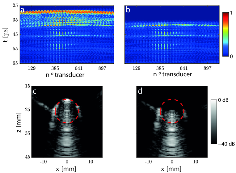
Figure S6: Time filtering of the specular sphere echo. a, Time evolution of the reflected wave-field $R_{0}(\mathbf{u}_{\textrm{out}},\bm{\theta}_{0},t)$ measured by the probe for the normal incident plane wave $\bm{\theta}_{0}=(0,0)$. b, Time evolution of the corresponding filtered wave-field $R^{\prime}_{0}(\mathbf{u}_{\textrm{out}},\bm{\theta}_{0},t)$. c, $(x,z)-$section of the confocal image $\mathcal{I}$ (Eq. 12) in the plane $y=y_{1}$ built from the free-space matrix $\mathbf{R}_{0}$. c, Same section of the confocal image $\mathcal{I}$ (Eq. 12) built from the filtered matrix $\mathbf{R}^{\prime}_{0}$. The data shown here are for sphere 1.

The importance of this filter is highlighted by comparing the likelihood index $\gamma$ built from $\mathbf{R}^{\prime}_{0}$ (Fig. S7a) and its initial counterpart (Fig. S5a). sphere 1 is now localized with a satisfying contrast $\mathcal{C}_{\gamma}=5.6$.

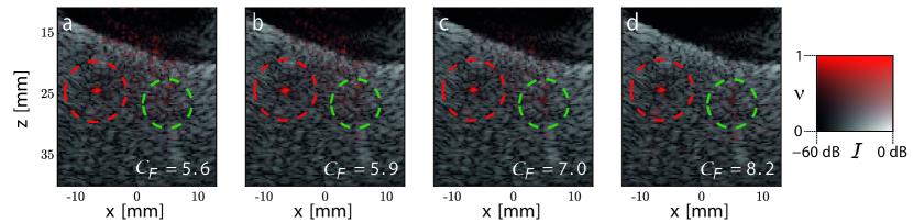
Figure S7: Optimization of the fingerprint operator. The $(x,z)-$cross-section ($y=y_{1}$) of the $\gamma-$map for sphere 1 (red scale) superimposed to the confocal image (B&W scale) is computed by considering as a fingerprint operator: a, the time filtered matrix ($\mathbf{F}=\mathbf{R}^{\prime}_{0}$); b, the $N_{1}$ first eigenstates of $\mathbf{R}^{\prime}_{0}$ $\left(\mathbf{F}=\sum_{p=1}^{N_{1}}\sigma_{p}\mathbf{U}_{p}\mathbf{V}_{p}^{{\dagger}}\right)$; c, after its singular spectrum whitening (Eq. 17); d, after the angular filtering described in Fig. S9. The frequency bandwidth is here 1.5-2.5 MHz.

To improve this contrast, a singular value decomposition can then be applied to the filtered matrix ${\mathbf{R}}^{\prime}_{0}(f)$ at each frequency $f$ (Eq. 16). The resulting singular values are displayed in Fig. S8. Only the eigenstates associated with singular values checking $\sigma_{i}>0.4\sigma_{1}$ can be considered to build the fingerprint operator. The resulting $\gamma-$map is displayed in Fig. S7b. The contrast improvement is modest ($\mathcal{C}_{\gamma}=5.9$) but is clearly improved after whitening the singular value spectrum (Eq. 17). The corresponding $\gamma-$map shown in Fig. S7c displays a contrast $\mathcal{C}_{\gamma}=7.0$.

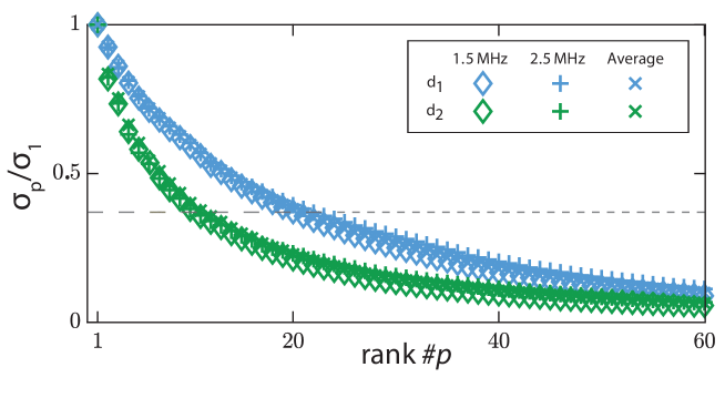
Figure S8: Singular values of the free-space and filtered matrices $\mathbf{R}^{\prime}_{0}(f)$ at frequency $f=1.5$ MHz and 2.5 MHz. Their values averaged over the frequency bandwidth is also displayed. The horizontal dashed line accounts for the threshold applied to build the fingerprint operator $\mathbf{F}$ in Eq. 17. Each singular value is normalized by its maximum value $\sigma_{1}$.

A last improvement consists in an angular decomposition of the fingerprint operator in order to filter the contribution of plane waves that cannot come from the target. This operation is illustrated by Fig. S9 and its result is shown in Fig. S7d. The final contrast $\mathcal{C}_{\gamma}$ reaches the excellent value of 8.2. Note that this value differs from the one reached in the accompanying paper (Fig. 3a, $\mathcal{C}_{\gamma}$) because the frequency bandwidth differs: 1.5-3.5 MHz in Fig. S7d vs. 1.8-2.6 MHz in Fig. 3a. In the former case, the frequency-averaged value of the scattering mean free path $\ell_{s}$ (Fig. S3) is larger than in the latter case.

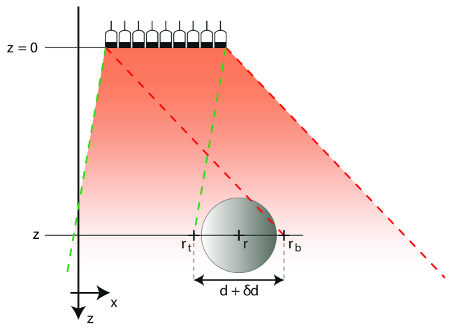
Figure S9: Scheme describing the selection of plane waves kept in the fingerprint operator. The orange area is a view of the selected angular sector. All the waves coming from outside this area are removed by the angular filter.

S3 Back-scattered wave-field by an elastic sphere

A COMSOL Multiphysics 6.0 simulation has been used to compute the wave-field scattered by the metal sphere. As the mechanical properties of the sphere used in the experiment are not known exactly, we use tabulated values for the simulation (Tab. S1). We also took advantage of the rotation symmetry of the sphere to use a two-dimensional axisymmetric simulation, which is less demanding in terms of resources and computing time. The aim of the simulation is first to estimate the field induced by the sphere when illuminated by an incident plane wave. In a second step, we will simulate focusing by coherently summing different plane waves obtained from the rotation of the initial plane wave simulation. The geometry, dimensions and physical quantities used for the simulation are all compiled in Fig. S10 and Tab. S1.

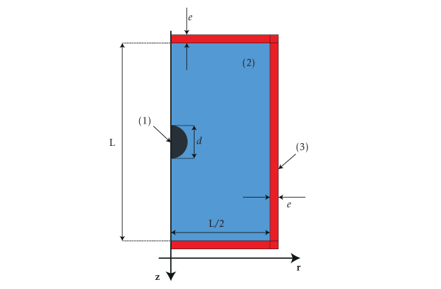
Figure S10: Numerical simulation of the sphere response. Scheme depicting the different parts of the simulation domain.

	Parameter	Value
Medium $(1)$	Medium	Isotropic Solid
	$d$	10
	$\rho_{b}$	5700
	$c_{\textrm{p}}$	2700
	$c_{\textrm{t}}$	2000
Medium $(2)$	Medium Type	Liquid
	$L$	60
	$\rho_{0}$	1000
	$c_{0}$	1500
Medium $(3)$	Medium	PML
	$e$	2,5
Simulation	Incident wave	Plane wave
	$f_{\textrm{min}}=\Delta f$	6
	$f_{\textrm{max}}$	6
	Frequency enveloppe	Hann window

Table S1: A set of parameters used to simulate the response of a metal sphere immersed in water in the presence of an incident plane wave.

Comsol simulation gives us access to a wide range of physical quantities both within the sphere and in the water. We have chosen to focus on the pressure in the water and the amplitude of the displacement field in the ball. These quantities are obtained for each frequency at any point in space. A Fourier transform is then computed after modulation by a Hann window to reconstruct a movie of wave propagation in the system in the plane $y=0$. Figure S11 shows the incident plane wave propagating through water until it is reflected by the sphere. In addition to being directly reflected, part of the wave is transmitted into the sphere, as two wave fronts emerge within it. The first, moving faster, corresponds to the longitudinal wave, while the second is associated with the transverse wave. In addition to these bulk waves, circumferential waves are also generated, corresponding to Rayleigh waves. These circulate along the surface and propagate without stopping, so that they can turn around the sphere.

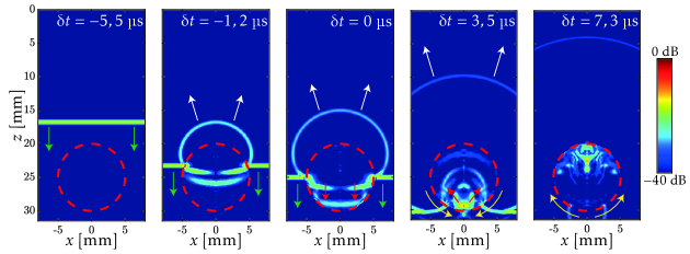
Figure S11: Wave propagation movie for an incident plane wave. Different snapshots are shown for an incident plane wave, observed in the $y=0$ plane. The incident wave propagates towards increasing $z$ (green arrows). Its interaction with the sphere gives rise to a specular back-refection (white arrows). Bulk waves are also generated within the sphere (red arrows). Finally, Rayleigh-type surface waves are also generated (yellow arrows). The time $\delta t=0$ corresponds to the passage of the plane wave through the $z=z_{0}$ plane (center of the sphere).

From this mother simulation, it is also possible to simulate focusing at any point of the simulation grid using the coherent sum of numerous plane waves. To simulate a three-dimensional focus from the parent simulation in axi-symmetric two-dimensional space, we rely on the rotation invariance of the system. To that aim, an observation grid is first defined for the simulated quantities. The idea is then to apply to the coordinates of this grid the rotation operation required to give the orientation of the wave vector of the parent simulation to the wave vector we are trying to simulate. For each plane wave to be simulated, we thus define a new associated grid that can be expressed in the cylindrical coordinates of the parent simulation. On each of these grids, the quantities of interest are finally estimated by interpolation from the grid of the parent simulation. At this stage, we now know the frequency dependence of the quantities of interest for all incident plane waves in a common grid.

S3.1 Origin of the bright tail

To form a confocal image from the parent simulation, the transducer coordinates of the matrix probe can be chosen as the acoustic pressure measurement grid. In this way, the reflection matrix of the simulated system can be computed. A confocal image can be deduced by applying a confocal beamforming process, as described in the Methods section and displayed in in Fig. S12. As already observed experimentally (Fig. 2e), the confocal image shows the sphere cap but also a bright tail, whose origin can now be investigated.

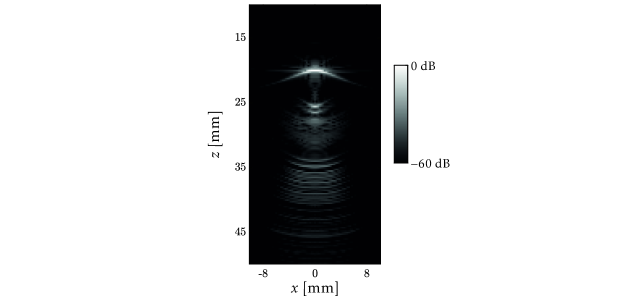
Figure S12: Confocal image obtained from the simulated reflection matrix. The $(x,z)-$section of the image is displayed in the plane $y=0$.

A film of wave propagation can be formed when all plane waves are suitably delayed to sum coherently at a point belonging to the bright tail. We are interested, for example, in the pixel $\mathbf{r}_{\textrm{in}}=(0;0;{25.5})$ mm and we set up an observation grid in the $y=0$ plane, on which we are now able to know the frequency dependence of the quantities of interest for the various incident plane waves. In order to focus on $\mathbf{r}_{\textrm{in}}$, it remains to apply beamforming in the frequency domain (Methods) so that all the plane waves sum coherently in $\mathbf{r}_{\textrm{in}}$ at the ballistic time ($\delta t=0$). The wave propagation movie is finally obtained by summing the wave-field obtained for each plane wave at each point $\mathbf{r}$ and then calculating the inverse time Fourier transform after bandwidth modulation by a Hann window.

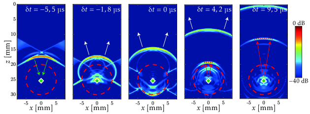
Figure S13: Wave propagation movie for an incident focused wave. Snapshots from the film of wave propagation in the system when focused on the point $\mathbf{r}_{\textrm{in}}=(0;0;{25.5})$ mm (green diamond) and observed in the plane $y=0$. The incident wave (green arrows) gradually converges towards $\mathbf{r}_{\textrm{in}}$. When the incident wave hits the sphere surface, a fraction of the energy is reflected (specular reflection, white arrows). Another fraction of the energy is converted into a whispering mode and then radiated back into the medium, (bulk reverberations, red arrows). The red dashed line represents the wave-front contributing to the reverberation observed in Fig. S12 at point $\mathbf{r}_{\textrm{in}}$.

Snapshots of this movie are displayed in Fig. S13. The incident focused wave does indeed appear to converge towards the point $\mathbf{r}_{\textrm{in}}$ as long as they propagate freely in the water. When they hit the surface of the ball, part of the energy is reflected, while another part is transmitted into the sphere. Longitudinal and transverse waves seem to undergo a refocusing process beneath the sphere surface and multiple reflections are observed at later time lapses. This process transfers a significant amount of energy back to the water, in the direction of the probe.

To form the confocal image, the echoes from $\mathbf{r}_{\textrm{in}}$ focus are precisely summed, selecting those corresponding to the supposed time delay between $\mathbf{r}_{\textrm{in}}$ and each transducer element. This echo highlighted by a red dashed line in Fig. S13 corresponds here to the first reflection on the back of the sphere. In the confocal image (Fig. S12), the bright tail thus exists thanks to the multiply-reflected bulk waves inside the sphere generated by incicent waves intended to focus at these points and then radiated back towards the probe with the time delay expected in a homogeneous medium.

S3.2 Origin of off-diagonal echoes

To better understand the origin of off-diagonal signal in the focused reflection matrix (Fig. 2d), we can once again rely on the simulation described above. Focused beamforming can be applied at input and output of the simulated reflection matrix in order to synthesize the focused reflection matrix at different depths (Method). As observed experimentally (Fig. 2d), we retrieve for certain depth strong off-diagonal echoes (Fig. S14).

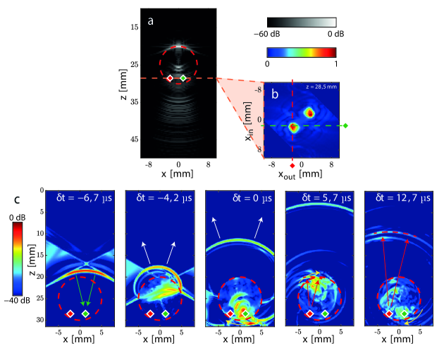
Figure S14: Origin of off-diagonal echoes. a, Confocal image in the $y=0$ plane. b, $x-$ cross-section of the focused reflection matrix in the focused basis in the plane $y_{\textrm{in}}=y_{\textrm{out}}=0$ and at depth $z=28.5$ mm. c, Snapshots of the wave propagation movie for an incident wave focusing on the point $\mathbf{r}_{\textrm{in}}=(1.25;0;28.5)$ mm (green diamond) and observed in the plane $y=0$. The incident wave-front (green arrows) gradually converges towards $\mathbf{r}_{\textrm{in}}$ . When the incident wave hits the surface, a fraction of the energy is reflected and gives rise to the specular echo (white arrows). Another fraction of the energy is converted into a circumferential surface wave (yellow arrows) and is then radiated back towards the probe (red arrows). The red dashed lines represent the echoes in the $y=0$ plane actually used by the probe to focus on the output point $\mathbf{r}_{\textrm{out}}=(-\bm{\rho_{\textrm{in}}},z)$ (red diamond). The chosen couple of points $(\mathbf{r}_{\textrm{in}},\mathbf{r}_{\textrm{out}})$ corresponds to the strong off-diagonal echo displayed in b.

Remarkably, the simulation once again allows us to track the origins of this off-diagonal echo, by simulating an incident wave focusing on the corresponding point $\mathbf{r}_{\textrm{in}}$. Snapshots of the corresponding movie are shown in Fig. S14c. It shows once again the incident wave converging towards the point $\mathbf{r}_{\textrm{in}}$ before hitting the sphere surface. A predominant surface wave is generated and propagates around the sphere (yellow arrow). The wave-front contributing to the off-diagonal echo in Fig. S14b is highlighted by a red dashed line. It indeed corresponds to the echo produced by the circumferential wave.

S4 Theoretical prediction of the target contrast

In the first experiment described in the accompanying paper (Fig. 1), the recorded reflection matrix $\mathbf{R}$ can be decomposed into a target component $\sigma_{T}\mathbf{R}_{0}$, and a multiple scattering contribution $\mathbf{M}$:

$$\mathbf{R}=\sigma_{T}\mathbf{R}_{0}+\mathbf{M}$$ (S4)

These two matrices are considered as fully uncorrelated. The single scattering contribution of the granular medium is neglected since multiple scattering is strongly predominant at the targets’ depths in Fig. 1. We will consider a normalized matrix $\mathbf{R}_{0}$ such that $\sigma_{T}$ accounts for the target signal:

$$\left\langle|R_{0}(\mathbf{u}_{\textrm{out}},\bm{\theta}_{\textrm{in}},f)|^{2}\right\rangle\equiv 1,$$

where the symbol $\langle\cdots\rangle$ stands for ensemble average.

S4.1 Target contrast in confocal imaging

Injecting Eq. 8 and 11 into Eq. 12 leads to the following expression for the mean confocal intensity:

$$\mathcal{I}=\left\langle\left|\frac{1}{\Delta f}\int_{f_{-}}^{f_{+}}df\sum_{\bm{\theta}_{\textrm{in}}}^{N_{\theta}}\sum_{\mathbf{u}_{\textrm{out}}}^{N_{u}}R(\mathbf{u}_{\textrm{out}},\bm{\theta}_{\textrm{in}},f)P^{*}(\bm{\rho},\bm{\theta}_{\textrm{in}},f)G^{*}(\bm{\rho},\mathbf{u}_{\textrm{out}},f)\right|^{2}\right\rangle.$$ (S5)

In the multiple scattering regime, confocal beamforming is an incoherent process: Each term in the triple sum of Eq. S5 can be seen as a random phasor. The corresponding multiple scattering contribution can be rewritten as follows:

$$\mathcal{I}_{M}=\frac{\delta f}{\Delta f}\sum_{\bm{\theta}_{\textrm{in}}}^{N_{\theta}}\sum_{\mathbf{u}_{\textrm{out}}}^{N_{u}}\left\langle\left|M(\mathbf{u}_{\textrm{out}},\bm{\theta}_{\textrm{in}},f)\right|^{2}\right\rangle$$ (S6)

where $\delta f$ is the correlation frequency of the multiple scattering noise. Let $\sigma_{M}^{2}=\left\langle\left|M(\mathbf{u}_{\textrm{out}},\bm{\theta}_{\textrm{in}},f)\right|^{2}\right\rangle$ be the power of multiple scattering noise recorded by the probe. The mean multiple scattering intensity thus scales as follows:

$$\mathcal{I}_{M}\sim\frac{N_{u}N_{\theta}}{N_{f}}\sigma_{M}^{2}$$ (S7)

with $N_{f}=\Delta f/\delta f$, the number of independent frequency grains in the frequency bandwidth. The confocal beamforming process amounts to increase the multiple scattering intensity by a factor $N_{\theta}$ due to the beamforming at input, by a factor $N_{u}$ due to the beamforming at output. Moreover, the different frequency components of the wave-field do not sum coherently which leads to a decrease of the multiple scattering intensity by the number $N_{f}$ of independent frequency grains in the bandwidth.

To derive an equivalent scaling for the target intensity, we will first consider the case of a point-like target. In that case, confocal beamforming is a perfectly coherent process with respect to the singly-scattered echo of the target: Each term in the triple sum of Eq. S5 adds constructively. The associated confocal intensity $\mathcal{I}_{P}$ thus scales as follows:

$$\mathcal{I}_{P}\sim{N_{\theta}^{2}N_{u}^{2}}\sigma_{T}^{2}$$ (S8)

The confocal beamforming process amounts to increase the point-like target intensity $\mathcal{I}_{P}$ by a factor $N_{\theta}^{2}$ due to the focused beamforming at input and by a factor $N_{u}^{2}$ due to the focused beamforming at output.

For a more complex target, the phasors in Eq. S5 are only partially coherent. This case is therefore intermediate between the multiple scattering component and the point-like target case. At each frequency, only one eigenstate of the reflection matrix, its specular component, leads to a coherent sum in the confocal beamforming process. If we assume that the target matrix exhibits a step-like distribution of singular values with $N_{S}$ the number of non-zero singular values, the confocal intensity should thus be decreased by a factor $N_{S}$ compared to the case point-like target. Moreover, the target exhibits a partially incoherent frequency spectrum. The associated intensity $\mathcal{I}_{T}$ will be also decreased by a factor $N_{T}$ compared to the point-like target case, $N_{T}$, being the number of independent coherence grains in the frequency bandwidth. The scaling $\mathcal{I}_{T}$ is therefore as follows:

$$\mathcal{I}_{T}\sim\frac{\mathcal{I}_{P}}{N_{S}N_{T}}\sim\frac{N_{\theta}^{2}N_{u}^{2}}{N_{S}N_{T}}\sigma_{T}^{2}$$ (S9)

where $N$ is the number of transducers. $N_{S}$ and $N_{T}$ are the number of spatial and temporal degrees of freedom exhibited by the target.

In the diffusive regime, the contrast between the direct echo of the target and the multiple scattering background in the confocal image is therefore given by:

$$\mathcal{C}_{I}=\frac{\mathcal{I}_{T}}{\mathcal{I}_{M}}\sim\frac{N_{\theta}N_{u}N_{f}}{N_{S}N_{T}}\frac{\sigma_{T}^{2}}{\sigma_{M}^{2}}$$ (S10)

S4.2 Target contrast provided by matrix fingerprint imaging

To evaluate the signal-to-noise ratio provided by the matrix fingerprint imaging process, we will consider Eq. 2 with a fingerprint operator equal to the target matrix: $\mathbf{F}=\mathbf{R}_{0}$. The mean intensity $\mathcal{F}$ of the fingerprint image is then given by:

$$\mathcal{F}=\beta^{-1}\left\langle\left|\frac{1}{\Delta f}\int_{f_{-}}^{f_{+}}df\sum_{\bm{\theta}_{\textrm{in}}}^{N_{\theta}}\sum_{\mathbf{u}_{\textrm{out}}}^{N_{u}}R(\mathbf{u}_{\textrm{out}},\bm{\theta}_{\textrm{in}},f)R_{0}^{*}(\mathbf{u}_{\textrm{out}},\bm{\theta}_{\textrm{in}},f)\right|^{2}\right\rangle$$ (S11)

where $\beta$ stands for the normalization factor of Eq. 2.

For the multiple scattering contribution, the associated mean intensity $\mathcal{F}_{M}$ can be computed by considering $\mathbf{R}=\mathbf{M}$ in Eq. S11

$$\mathcal{F}_{M}=\beta^{-1}\left\langle\left|\frac{1}{\Delta f}\int_{f_{-}}^{f_{+}}df\sum_{\bm{\theta}_{\textrm{in}}}^{N_{\theta}}\sum_{\mathbf{u}_{\textrm{out}}}^{N_{u}}M(\mathbf{u}_{\textrm{out}},\bm{\theta}_{\textrm{in}},f)R_{0}^{*}(\mathbf{u}_{\textrm{out}},\bm{\theta}_{\textrm{in}},f)\right|^{2}\right\rangle$$ (S12)

The reflection matrix coefficients of the multiple scattering contribution and of the target component are fully uncorrelated. The triple sum is therefore incoherent in Eq. S12 :

$$\mathcal{F}_{M}=\beta^{-1}\frac{1}{N_{f}}\sum_{\bm{\theta}_{\textrm{in}}}^{N_{\theta}}\sum_{\mathbf{u}_{\textrm{out}}}^{N_{u}}\left\langle|M(\mathbf{u}_{\textrm{out}},\bm{\theta}_{\textrm{in}},f)|^{2}\right\rangle\left\langle|R_{0}(\mathbf{u}_{\textrm{out}},\bm{\theta}_{\textrm{in}},f)|^{2}\right\rangle$$ (S13)

which simplifies into:

$$\mathcal{F}_{M}\sim\frac{N_{\theta}N_{u}}{\beta N_{f}}\sigma_{M}^{2}$$ (S14)

For the target contribution, the associated fingerprint intensity $\mathcal{F}_{T}$ can be derived by considering $\mathbf{R}=\sigma_{T}\mathbf{R}_{0}$ in Eq. S11:

$$\mathcal{F}_{T}=\frac{\sigma_{T}^{2}}{\beta}\left\langle\left|\frac{1}{\Delta f}\int_{f_{-}}^{f_{+}}df\sum_{\bm{\theta}_{\textrm{in}}}^{N_{\theta}}\sum_{\mathbf{u}_{\textrm{out}}}^{N_{u}}\left|R_{0}(\mathbf{u}_{\textrm{out}},\bm{\theta}_{\textrm{in}},f)\right|^{2}\right|^{2}\right\rangle$$ (S15)

Each term in the triple sum is coherent, which yields the following scaling for the target intensity $\mathcal{F}_{T}$:

$$\mathcal{F}_{T}\sim\frac{N_{\theta}^{2}N_{u}^{2}}{\beta}\sigma_{T}^{2}$$ (S16)

The contrast between the target signal with respect to the multiple scattering background (Eq. S14) in the likelihood image is therefore given by:

$$\mathcal{C}_{\gamma}=\frac{\mathcal{F}_{T}}{\mathcal{F}_{M}}\sim N_{\theta}N_{u}N_{f}\frac{\sigma_{T}^{2}}{\sigma_{M}^{2}}$$ (S17)

Compared to the confocal image (Eq. S10), the gain $G$ provided by the fingerprint operator in terms of contrast between the target and the multiple scattering fog scales as:

$$G=\frac{\mathcal{C}_{\gamma}}{\mathcal{C}_{I}}\sim N_{S}N_{T}$$ (S18)

$G$ corresponds to the number of spatial and temporal d.o.f exhibited by the target echo.

S5 Precision of the localization process

As shown by Desailly and colleagues ³⁸ in the context of ultrasound localization microscopy ⁵², the transverse and axial localization precision can be expressed by means of the Cramér-Rao bound as follows:

$$\delta\rho_{L}\sim 2\sqrt{3}\frac{\sigma_{t}}{f_{c}}\frac{\delta\rho_{D}}{\sqrt{N_{u}N_{\theta}}}$$ (S19)

and

$$\delta z_{L}\sim\frac{c\sigma_{t}}{2}\frac{1}{\sqrt{N_{u}N_{\theta}}}$$ (S20)

where $\sigma_{t}$ is the standard deviation $\sigma_{t}$ of echo time estimates. This quantity has been derived in a seminal paper by Quazi for a limited bandwidth ($\Delta f\ll f_{c}$) ³⁷:

$$\sigma_{t}=\frac{1}{2\sqrt{2}\pi}\sqrt{\frac{\sigma_{M}}{\sigma_{T}}}\frac{f_{c}}{\sqrt{N_{f}}}$$ (S21)

Injecting Eq. S21 into Eq. S19 leads to the following expression for $\delta\rho_{L}$:

$$\delta\rho_{L}\sim\frac{1}{\pi}\sqrt{\frac{3}{2}}\sqrt{\frac{\sigma_{M}}{\sigma_{T}}}\frac{\delta\rho_{D}}{\sqrt{N_{f}N_{u}N_{\theta}}}$$ (S22)

Using Eq. S17, the previous equation can be recast as follows:

$$\delta\rho_{L}\sim\frac{1}{\pi}\sqrt{\frac{3}{2}}\frac{\delta\rho_{D}}{\sqrt{\mathcal{C}_{\gamma}}}$$ (S23)

As regards to the axial resolution $\delta z_{L}$, Eqs. S21 and S17 can be injected into Eq. S20 to obtain:

$$\delta z_{L}\sim\frac{1}{4\sqrt{2}\pi}\frac{cf_{c}}{\sqrt{\mathcal{C}_{\gamma}}}$$ (S24)

The transverse and axial precision of the localization process are therefore inversely proportional to the target contrast. This fundamental result shows the benefit of the fingerprint operator for localization purposes.

References

- Fink [1997] M. Fink, Time reversed acoustics, Physics Today 50, 34 (1997).
- Mosk et al. [2012] A. P. Mosk, A. Lagendijk, G. Lerosey, and M. Fink, Controlling waves in space and time for imaging and focusing in complex media, Nat. Photonics 6, 283 (2012).
- Foschini and Gans [1998] G. Foschini and M. Gans, On limits of wireless communications in a fading environment when using multiple antennas, Wireless Personal Communications 6, 311 (1998).
- Popoff et al. [2010] S. M. Popoff, G. Lerosey, R. Carminati, M. Fink, A. C. Boccara, and S. Gigan, Measuring the transmission matrix in optics: An approach to the study and control of light propagation in disordered media, Phys. Rev. Lett. 104, 100601 (2010).
- Prada and Fink [1994] C. Prada and M. Fink, Eigenmodes of the time reversal operator: A solution to selective focusing in multiple-target media, Wave Motion 20, 151 (1994).
- Popoff et al. [2011] S. M. Popoff, A. Aubry, G. Lerosey, M. Fink, A. C. Boccara, and S. Gigan, Exploiting the time-reversal operator for adaptive optics, selective focusing, and scattering pattern analysis, Phys. Rev. Lett. 107, 263901 (2011).
- Rotter and Gigan [2017] S. Rotter and S. Gigan, Light fields in complex media: Mesoscopic scattering meets wave control, Rev. Mod. Phys. 89, 015005 (2017).
- Cao et al. [2022] H. Cao, A. P. Mosk, and S. Rotter, Shaping the propagation of light in complex media, Nat. Phys. 18, 994 (2022).
- Bertolotti and Katz [2022] J. Bertolotti and O. Katz, Imaging in complex media, Nat. Phys. 18, 1008 (2022).
- Gérardin et al. [2014] B. Gérardin, J. Laurent, A. Derode, C. Prada, and A. Aubry, Full transmission and reflection of waves propagating through a maze of disorder, Phys. Rev. Lett. 113, 173901 (2014).
- Popoff et al. [2014] S. M. Popoff, A. Goetschy, S. F. Liew, A. D. Stone, and H. Cao, Coherent Control of Total Transmission of Light through Disordered Media, Phys. Rev. Lett. 112, 133903 (2014).
- Davy et al. [2015] M. Davy, Z. Shi, J. Park, C. Tian, and A. Z. Genack, Universal structure of transmission eigenchannels inside opaque media, Nat. Commun. 6, 6893 (2015).
- Aubry and Derode [2009] A. Aubry and A. Derode, Detection and imaging in a random medium: A matrix method to overcome multiple scattering and aberration, J. Appl. Phys. 106, 044903 (2009).
- Badon et al. [2016] A. Badon, D. Li, G. Lerosey, A. C. Boccara, M. Fink, and A. Aubry, Smart optical coherence tomography for ultra-deep imaging through highly scattering media, Sci. Adv. 2, e1600370 (2016).
- Aubry et al. [2006] A. Aubry, J. de Rosny, J.-G. Minonzio, C. Prada, and M. Fink, Gaussian beams and legendre polynomials as invariants of the time reversal operator for a large rigid cylinder, J. Acoust. Soc. Am. 120, 2746 (2006).
- Robert and Fink [2009] J.-L. Robert and M. Fink, The prolate spheroidal wave functions as invariants of the time reversal operator for an extended scatterer in the Fraunhofer approximation, J. Acoust. Soc. Am. 125, 218 (2009).
- Yoon et al. [2020] S. Yoon, H. Lee, J. H. Hong, Y.-S. Lim, and W. Choi, Laser scanning reflection-matrix microscopy for aberration-free imaging through intact mouse skull, Nat. Commun. 11, 5721 (2020).
- Jo et al. [2022] Y. Jo, Y.-R. Lee, J. H. Hong, D.-Y. Kim, J. Kwon, M. Choi, M. Kim, and W. Choi, Through-skull brain imaging in vivo at visible wavelengths via dimensionality reduction adaptive-optical microscopy, Sci. Adv. 8, eabo4366 (2022).
- Lee et al. [2022] H. Lee, S. Yoon, P. Loohuis, J. H. Hong, S. Kang, and W. Choi, High-throughput volumetric adaptive optical imaging using compressed time-reversal matrix, Light Sci Appl 11, 16 (2022).
- Weinberg et al. [2024] G. Weinberg, E. Sunray, and O. Katz, Noninvasive megapixel fluorescence microscopy through scattering layers by a virtual incoherent reflection matrix, Sci. Adv. 10, eadl5218 (2024).
- Badon et al. [2020] A. Badon, V. Barolle, K. Irsch, A. C. Boccara, M. Fink, and A. Aubry, Distortion matrix concept for deep optical imaging in scattering media, Sci. Adv. 6, eaay7170 (2020).
- Lambert et al. [2020a] W. Lambert, L. A. Cobus, T. Frappart, M. Fink, and A. Aubry, Distortion matrix approach for ultrasound imaging of random scattering media, Proc. Nat. Acad. Sci. 117, 14645 (2020a).
- Bureau et al. [2023] F. Bureau, J. Robin, A. Le Ber, W. Lambert, M. Fink, and A. Aubry, Three-dimensional ultrasound matrix imaging, Nat. Commun. 14, 6793 (2023).
- Murray et al. [2023] G. Murray, J. Field, M. Xiu, Y. Farah, L. Wang, O. Pinaud, and R. Bartels, Aberration free synthetic aperture second harmonic generation holography, Opt. Express 31, 32434 (2023).
- Giraudat et al. [2024] E. Giraudat, A. Burtin, A. Le Ber, M. Fink, J.-C. Komorowski, and A. Aubry, Matrix imaging as a tool for high-resolution monitoring of deep volcanic plumbing systems with seismic noise, Commun. Earth Environ. 5, 509 (2024).
- Zhang et al. [2023] Y. Zhang, M. Dinh, Z. Wang, T. Zhang, T. Chen, and C. W. Hsu, Deep imaging inside scattering media through virtual spatiotemporal wavefront shaping, arXiv:2306.08793 10.48550/ARXIV.2306.08793 (2023).
- Najar et al. [2024] U. Najar, V. Barolle, P. Balondrade, M. Fink, C. Boccara, and A. Aubry, Harnessing forward multiple scattering for optical imaging deep inside an opaque medium, Nat. Commun. 15, 7349 (2024).
- Pai et al. [2021] P. Pai, J. Bosch, M. Kühmayer, S. Rotter, and A. P. Mosk, Scattering invariant modes of light in complex media, Nat. Photon. 15, 431 (2021).
- van den Wildenberg et al. [2019] S. van den Wildenberg, X. Jia, J. Léopoldès, and A. Tourin, Ultrasonic tracking of a sinking ball in a vibrated dense granular suspension, Sci. Rep. 9, 5460 (2019).
- Goïcoechea et al. [2024] A. Goïcoechea, C. Brütt, A. Le Ber, F. Bureau, W. Lambert, C. Prada, A. Derode, and A. Aubry, Reflection measurement of the scattering mean free path at the onset of multiple scattering, Phys. Rev. Lett. 133, 176301 (2024).
- Thomas et al. [1994] J.-L. Thomas, P. Roux, and M. Fink, Inverse scattering analysis with an acoustic time-reversal mirror, Phys. Rev. Lett. 72, 637 (1994).
- Prada and Fink [1998] C. Prada and M. Fink, Separation of interfering acoustic scattered signals using the invariants of the time-reversal operator. application to lamb waves characterization, J. Acoust. Soc. Am. 104, 801 (1998).
- Gespa and Überall [1987] N. Gespa and H. Überall, La Diffusion Acoustique Par Des Cibles Élastiques de Forme Géométrique Simple: Théories Et Expériences (CEDOCAR, 1987).
- Royer et al. [1988] D. Royer, E. Dieulesaint, X. Jia, and Y. Shui, Optical generation and detection of surface acoustic waves on a sphere, Appl. Phys. Lett. 52, 706 (1988).
- Clorennec and Royer [2004] D. Clorennec and D. Royer, Investigation of surface acoustic wave propagation on a sphere using laser ultrasonics, Appl. Phys. Lett. 85, 2435 (2004).
- Lambert et al. [2020b] W. Lambert, L. A. Cobus, M. Couade, M. Fink, and A. Aubry, Reflection matrix approach for quantitative imaging of scattering media, Phys. Rev. X 10, 021048 (2020b).
- Quazi [1981] A. Quazi, An overview on the time delay estimate in active and passive systems for target localization, IEEE Transactions on Acoustics, Speech, and Signal Processing 29, 527 (1981).
- Desailly et al. [2015] Y. Desailly, J. Pierre, O. Couture, and M. Tanter, Resolution limits of ultrafast ultrasound localization microscopy, Phys. Med. Biol. 60, 8723 (2015).
- Rüland et al. [2018] A. M. Rüland, F. Hagemann, M. Reinisch, J. Holtschmidt, A. Kümmel, C. Dittmer-Grabowski, F. Stöblen, H. Rotthaus, V. Dreesmann, J.-U. Blohmer, and S. Kümmel, Using a new marker clip system in breast cancer: Tumark vision clip - feasibility testing in everyday clinical practice, Breast Care 13, 114 (2018).
- Wijntjes and van Alfen [2020] J. Wijntjes and N. van Alfen, Muscle ultrasound: Present state and future opportunities, Muscle & Nerve 63, 455 (2020).
- Papadacci et al. [2017] C. Papadacci, V. Finel, J. Provost, O. Villemain, P. Bruneval, J.-L. Gennisson, M. Tanter, M. Fink, and M. Pernot, Imaging the dynamics of cardiac fiber orientation in vivo using 3d ultrasound backscatter tensor imaging, Sci. Rep. 7, 830 (2017).
- Rodriguez-Molares et al. [2017] A. Rodriguez-Molares, A. Fatemi, L. Lovstakken, and H. Torp, Specular Beamforming, IEEE Trans. Ultrason. Ferroelectr. Freq. Control 64, 1285 (2017).
- Tseng et al. [2005] W. I. Tseng, J. Dou, T. G. Reese, and V. J. Wedeen, Imaging myocardial fiber disarray and intramural strain hypokinesis in hypertrophic cardiomyopathy with mri, Journal of Magnetic Resonance Imaging 23, 1 (2005).
- Thompson et al. [2008] R. B. Thompson, F. Margetan, P. Haldipur, L. Yu, A. Li, P. Panetta, and H. Wasan, Scattering of elastic waves in simple and complex polycrystals, Wave Motion 45, 655 (2008).
- Holmes et al. [2018] D. F. Holmes, Y. Lu, T. Starborg, and K. E. Kadler, Collagen fibril assembly and function, in Extracellular Matrix and Egg Coats (Elsevier, 2018) pp. 107–142.
- Raoux et al. [2023] C. Raoux, A. Chessel, P. Mahou, G. Latour, and M.-C. Schanne-Klein, Unveiling the lamellar structure of the human cornea over its full thickness using polarization-resolved shg microscopy, Light Sci. Appl. 12, 190 (2023).
- Balondrade et al. [2024] P. Balondrade, V. Barolle, N. Guigui, E. Auriant, N. Rougier, C. Boccara, M. Fink, and A. Aubry, Multi-spectral reflection matrix for ultrafast 3d label-free microscopy, Nat. Photon. 18, 1097 (2024).
- Ammari et al. [2013] H. Ammari, T. Boulier, J. Garnier, W. Jing, H. Kang, and H. Wang, Target identification using dictionary matching of generalized polarization tensors, Fond. Comput. Math. 14, 27 (2013).
- Ammari et al. [2014] H. Ammari, M. P. Tran, and H. Wang, Shape identification and classification in echolocation, Siam. J. Imaging Sci. 7, 1883 (2014).
- De Jong et al. [2002] N. De Jong, A. Bouakaz, and P. Frinking, Basic acoustic properties of microbubbles, Echocardiography 19, 229 (2002).
- Tremblay-Darveau et al. [2014] C. Tremblay-Darveau, R. Williams, and P. N. Burns, Measuring absolute blood pressure using microbubbles, Ultrasound Med. Biol. 40, 775 (2014).
- Errico et al. [2015] C. Errico, J. Pierre, S. Pezet, Y. Desailly, Z. Lenkei, O. Couture, and M. Tanter, Ultrafast ultrasound localization microscopy for deep super-resolution vascular imaging, Nature 527, 499 (2015).
- Chavignon et al. [2022] A. Chavignon, V. Hingot, C. Orset, D. Vivien, and O. Couture, 3d transcranial ultrasound localization microscopy for discrimination between ischemic and hemorrhagic stroke in early phase, Sci. Rep. 12, 14607 (2022).
- Xu et al. [2008] L. Xu, J. Li, and P. Stoica, Target detection and parameter estimation for mimo radar systems, IEEE Trans. Aerosp. Electron. Syst. 44, 927 (2008).
- Pailhas et al. [2017] Y. Pailhas, J. Houssineau, Y. R. Petillot, and D. E. Clark, Tracking with mimo sonar systems: applications to harbour surveillance, IET Radar Sonar Navig. 11, 629 (2017).
- Guck et al. [2005] J. Guck, S. Schinkinger, B. Lincoln, F. Wottawah, S. Ebert, M. Romeyke, D. Lenz, H. M. Erickson, R. Ananthakrishnan, D. Mitchell, J. Käs, S. Ulvick, and C. Bilby, Optical deformability as an inherent cell marker for testing malignant transformation and metastatic competence, Biophys. J. 88, 3689 (2005).
- Zhang et al. [2017] Q. Zhang, L. Zhong, P. Tang, Y. Yuan, S. Liu, J. Tian, and X. Lu, Quantitative refractive index distribution of single cell by combining phase-shifting interferometry and AFM imaging, Sci. Rep. 7, 2532 (2017).
- Janmey et al. [2020] P. A. Janmey, D. A. Fletcher, and C. A. Reinhart-King, Stiffness sensing by cells, Physiol. Rev. 100, 695 (2020).
- Barolle et al. [2024] V. Barolle, F. Bureau, N. Guigui, P. Balondrade, V. Brochard, O. Dubois, A. Jouneau, A. Bonnet-Garnier, and A. Aubry, Optical matrix imaging applied to embryology, arXiv:2410.11126 10.48550/ARXIV.2410.11126 (2024).
- Harrison et al. [2021] S. P. Harrison, S. F. Baumgarten, R. Verma, O. Lunov, A. Dejneka, and G. J. Sullivan, Liver organoids: Recent developments, limitations and potential, Front. Med. 8, 10.3389/fmed.2021.574047 (2021).
- Montaldo et al. [2009] G. Montaldo, M. Tanter, J. Bercoff, N. Benech, and M. Fink, Coherent plane-wave compounding for very high frame rate ultrasonography and transient elastography, IEEE Trans. Ultrason. Ferroelectr. Freq. Control 56, 489 (2009).
- Le Ber et al. [2024] A. Le Ber, A. Goicoechea, W. Lambert, X. Jia, A. Tourin, and A. Aubry, Fingerprint matrix imaging [data]. Zenodo (2024).
- Page et al. [1996] J. H. Page, P. Sheng, H. P. Schriemer, I. Jones, J. Xiaodun, and D. A. Weitz, Group Velocity in Strongly Scattering Media, Science 271, 634 (1996).
- Le Ber [2024] A. Le Ber, Approche matricielle de la propagation des ultrasons dans les suspensions granulaires, Ph.D. thesis, PSL University (2024).
- Page et al. [1995] J. H. Page, H. P. Schriemer, A. E. Bailey, and D. A. Weitz, Experimental test of the diffusion approximation for multiply scattered sound, Phys. Rev. E 52, 3106 (1995).
- Jia [2004] X. Jia, Codalike multiple scattering of elastic waves in dense granular media, Phys. Rev. Lett. 93, 154303 (2004).