A Closed-Form Transition Density Expansion for Elliptic and Hypo-Elliptic SDEs

Abstract

We introduce a closed-form expansion for the transition density of elliptic and hypo-elliptic multivariate Stochastic Differential Equations (SDEs), over a period $\displaystyle\Delta\in(0,1)$, in terms of powers of $\displaystyle\Delta^{j/2}$, $\displaystyle j\geq 0$. Our methodology provides approximations of the transition density, easily evaluated via any software that performs symbolic calculations. A major part of the paper is devoted to an analytical control of the remainder in our expansion for fixed $\displaystyle\Delta\in(0,1)$. The obtained error bounds validate theoretically the methodology, by characterising the size of the distance from the true value. It is the first time that such a closed-form expansion becomes available for the important class of hypo-elliptic SDEs, to the best of our knowledge. For elliptic SDEs, closed-form expansions are available, with some works identifying the size of the error for fixed $\displaystyle\Delta$, as per our contribution. Our methodology allows for a uniform treatment of elliptic and hypo-elliptic SDEs, when earlier works are intrinsically restricted to an elliptic setting. We show numerical applications highlighting the effectiveness of our method, by carrying out parameter inference for hypo-elliptic SDEs that do not satisfy stated conditions. The latter are sufficient for controlling the remainder terms, but the closed-form expansion itself is applicable in general settings.

1 Introduction

Stochastic Differential Equations (SDEs) constitute an effective tool for modelling non-linear dynamics that arise in numerous application fields, including, e.g., finance, physics and neuroscience (Kloeden and Platen, 1992). Over the past few decades, a large amount of research has contributed to methodological and theoretical advances on the theme of parameter inference for SDEs. An overarching challenge is that the transition density of a non-linear SDE is in general intractable, thus appropriate proxies must be formulated to conduct likelihood-based inference. We propose a new closed-form (CF) transition density expansion for SDEs, which can approximate the true density with high precision. In contrast to previous approaches, one of the novelties of our methodology is that it covers a broad class of diffusion processes, including hypo-elliptic SDEs, i.e. processes with a degenerate diffusion matrix and a transition law that still admits a density with respect to (w.r.t.) the Lebesgue measure. Hypo-elliptic SDEs appear in broad areas of applications (including physics, neuroscience) and parameter inference for these models has been a very active area of research in the last years.

Let $\displaystyle B_{t}=(B_{1,t},\ldots,B_{d,t})$, $\displaystyle t\geq 0$, be the standard $\displaystyle d$-dimensional Brownian motion, $\displaystyle d\geq 1$, defined upon the filtered probability space $\displaystyle(\Omega,\mathcal{F},\{\mathcal{F}_{t}\}_{t\geq 0},\mathbb{P})$. We consider $\displaystyle N$-dimensional SDEs, $\displaystyle N\geq 1$, of the following general form:

$$\displaystyle dX_{t}=V_{0}(X_{t},\theta)\,dt+\sum_{1\leq j\leq d}V_{j}(X_{t},\theta)\,dB_{j,t},\quad X_{0}=x_{0}\in\mathbb{R}^{N},$$ (1.1)

for parameter vector $\displaystyle\theta\in\Theta\subseteq\mathbb{R}^{N_{\theta}}$, $\displaystyle N_{\theta}\geq 1$, and functions $\displaystyle V_{j}:\mathbb{R}^{N}\times\Theta\to\mathbb{R}^{N},\,0\leq j\leq d$. We set $\displaystyle\sigma=[V_{1},\ldots,V_{d}]$ and $\displaystyle a=\sigma\sigma^{\top}$. Our work focuses on two model classes, covering a large set of SDEs used in applications. The first class is the elliptic one, where we consider SDEs of the following form:

$$\displaystyle\begin{aligned} dX_{t}=V_{R,0}(X_{t},\theta)dt+\sum_{1\leq j\leq d}V_{R,j}(X_{t},\theta)dB_{j,t},\quad X_{0}=x_{0}\in\mathbb{R}^{N},\end{aligned}$$ (E)

so that $\displaystyle V_{j}=V_{R,j}$, $\displaystyle 0\leq j\leq d$. We set $\displaystyle\sigma_{R}=[V_{R,1},\ldots,V_{R,d}]$, $\displaystyle a_{R}=\sigma_{R}\sigma_{R}^{\top}$, and assume that $\displaystyle a_{R}=a_{R}(x,\theta)$ is positive definite for all $\displaystyle(x,\theta)\in\mathbb{R}^{N}\times\Theta$. Thus, w.l.o.g. here $\displaystyle d=N$. Class (E) includes a multitude of models used in applications, see e.g. Kloeden and Platen (1992). The second model class we work with is the hypo-elliptic one, where the SDE in (1.1) now splits into smooth and rough components as $\displaystyle X_{t}=(X_{S,t},X_{R,t})\in\mathbb{R}^{N_{S}+N_{R}}$, so that $\displaystyle N=N_{S}+N_{R}$, $\displaystyle N_{S}\geq 1$, $\displaystyle N_{R}\geq 1$, and we re-express (1.1) as:

$$\displaystyle\begin{aligned} dX_{S,t}&=V_{S,0}(X_{t},\theta)\,dt;\qquad dX_{R,t}=V_{R,0}(X_{t},\theta)\,dt+\sum_{1\leq j\leq d}V_{R,j}(X_{t},\theta)\,dB_{j,t},\\ X_{0}&=x_{0}=(x_{S,0},x_{R,0})\in\mathbb{R}^{N_{S}+N_{R}}.\end{aligned}$$ (H)

In (H), the involved functions are defined as $\displaystyle V_{S,0}:\mathbb{R}^{N}\times\Theta\to\mathbb{R}^{N_{S}},\,V_{R,j}:\mathbb{R}^{N}\times\Theta\to\mathbb{R}^{N_{R}},\,0\leq j\leq d.$ Model class (H) stems from the generic form (1.1), where we now have that, for $\displaystyle(x,\theta)\in\mathbb{R}^{N}\times\Theta$:

$$\displaystyle V_{0}(x,\theta)=\bigl{[}V_{S,0}(x,\theta)^{\top},V_{R,0}(x,\theta)^{\top}\bigr{]}^{\top},\qquad V_{j}(x,\theta)=\bigl{[}\mathbf{0}_{N_{S}}^{\top},V_{R,j}(x,\theta)^{\top}\bigr{]}^{\top},\qquad 1\leq j\leq d.$$

Notice that component $\displaystyle X_{S,t}$ is not driven by the Brownian motion, and consequently class (H) requires a separate treatment from (E). Later on, we introduce sufficient requirements associated with the weak Hörmander’s condition, so that $\displaystyle V_{S,0}(X_{t},\theta)$ depends on $\displaystyle X_{R,t}$, thus Brownian noise propagates into the smooth component, and the law of $\displaystyle X_{t}$, $\displaystyle t>0$, admits a density w.r.t. the Lebesgue measure. Hypo-elliptic models are used in several application fields, including, e.g.: the FitzHugh-Nagumo SDE (DeVille et al., 2005) and the Jansen-Rit neural mass SDE (Ableidinger et al., 2017) in neuroscience; the underdamped or generalised Langevin equation (Pavliotis, 2014) in physics.

We consider parameter inference for SDEs given a collection of discrere-time data $\displaystyle\{X_{t}\}_{t\in\mathbb{T}_{n}}$, for the set of time instances $\displaystyle\mathbb{T}_{n}=\{t_{0},t_{1},\ldots,t_{n}\}$, $\displaystyle n\geq 1$. For simplicity, we consider equidistant step-sizes, with $\displaystyle\Delta:=t_{i}-t_{i-1}$. The likelihood function is given as:

$$L_{n}(\{X_{t}\}_{t\in\mathbb{T}_{n}};\theta)=p(X_{t_{0}};\theta)\prod_{1\leq i\leq n}p_{\Delta}^{X}(X_{t_{i-1}},X_{t_{i}};\theta),$$

for some initial law $\displaystyle p(\cdot;\theta)$, where $\displaystyle x^{\prime}\mapsto p_{\Delta}^{X}(x,x^{\prime};\theta)$ is the transition density of SDE (1.1), with the latter being in general unavailable in closed form. A practical standard approach to circumvent this intractability is by introducing a time-discretisation scheme and using the induced CF approximate transition density as a proxy for the true one. For instance, a common scheme is the Euler-Maruyama one, which yields a conditionally Gaussian approximate density upon application to elliptic SDEs. However, it is well-understood that such an approximation cannot correctly capture the true non-linear dynamics unless the step-size $\displaystyle\Delta$ is close to $\displaystyle 0$. Thus, parameter estimation relying on such a simple Gaussian approximation requires a high-frequency observation regime, with $\displaystyle\Delta\ll 1$. In practice, the step-size of available data is usually fixed, and its value may not be too small.

In the context of fixed $\displaystyle\Delta$, the prominent work of Aït-Sahalia (2002) proposes an elaborate approximation of the transition density for time-homogeneous univariate elliptic SDEs via a CF Hermite-series expansion. Roughly, the expansion for the transition density is of the structure:

$$\displaystyle{p_{\Delta}^{X}(x,y;\theta)}\approx{q_{\Delta}(x,y;\theta)\times\bigl{\{}1+(\mathrm{correction\,term})\bigr{\}}}.$$ (1.2)

Here, $\displaystyle y\mapsto q_{\Delta}(x,y;\theta)$ is a ‘baseline’ tractable density. The ‘correction term’ is given in closed-form, and includes Hermite polynomials up to a degree $\displaystyle J\geq 1$, obtained via working with $\displaystyle q_{\Delta}(x,y;\theta)$. The correction term plays a key role in capturing non-linear/non-Gaussian effects in the true transitions. In detail, Aït-Sahalia (2002) constructs the CF-expansion by first applying an 1–1 ‘Lamperti transform’ (Roberts and Stramer, 2001), thus replacing the original scalar $\displaystyle X_{t}$ with a process $\displaystyle Y_{t}$ of unit diffusion coefficient, and then obtaining the Hermite series expansion for the transition density of $\displaystyle Y_{t}$. We refer to this line of research as the Hermite approach. Aït-Sahalia (2002) proves convergence of the CF-expansion to the true density for fixed $\displaystyle\Delta\in(0,1)$ as the degree of Hermite polynomials, $\displaystyle J$, grows to infinity. The result is a qualitative one, as no order of convergence is provided. The Hermite approach works only for the sub-class of ‘reducible’ elliptic SDEs for which the Lamperti transform is applicable. Also, as stated in Aït-Sahalia (2008), convergence of the Hermite series expansion is not guaranteed when back-transforming onto the original density of $\displaystyle X_{t}$. To treat a wider class of non-reducible multivariate elliptic SDEs, Aït-Sahalia (2008) utilises the Kolmogorov backward/forward equations (PDEs) to construct a series expansion in $\displaystyle\Delta$ and $\displaystyle y-x$. No analytical results are provided for fixed $\displaystyle\Delta$. We refer to this contribution as the PDE approach. Li (2013) develops a probabilistic approach, by making use of Malliavin calculus and carrying out an asymptotic analysis of Wiener functionals (Watanabe, 1987; Yoshida, 1992) to obtain a CF-expansion, accompanied by an analytic bound for the approximation error, for fixed $\displaystyle\Delta$. The expansion is given in terms of powers $\displaystyle\Delta^{j/2}$, $\displaystyle j\geq 0$, for $\displaystyle\Delta\in(0,1)$. More precisely:

$$\displaystyle p_{\Delta}^{X}(x,y;\theta)=q_{\Delta}(x,y;\theta)\times\Bigl{\{}1+\sum_{1\leq j\leq J}\Delta^{j/2}\cdot e^{(j)}_{\Delta}(x,y;\theta)\Bigr{\}}+R(\Delta,x,y;\theta),\qquad J\geq 1,$$ (1.3)

for tractable coefficients $\displaystyle e_{\Delta}^{(j)}(\cdot)$, $\displaystyle j\geq 1$, and a remainder term $\displaystyle R(\cdot)$. Li (2013) proves under conditions that the remainder is of size $\displaystyle\mathcal{O}(\Delta^{(J+1-N)/2})$. The probabilistic approach is extended to elliptic SDEs with jumps in Li and Chen (2016). For time-inhomogeneous elliptic SDEs, Choi (2015) develops a CF-expansion via the PDE approach, similarly to Aït-Sahalia (2008). Yang et al. (2019) use Itô-Taylor expansions and obtain a series of the form (1.3) that involves Hermite polynomials, with explicit bounds provided on residuals as in Li (2013). Even if alternative approaches have been followed in the literature, the produced expansions are closely related to each other. E.g., one can obtain a series expansion as in (1.3) involving Hermite polynomials via the two different approaches in Li (2013); Yang et al. (2019). Furthermore, Lee et al. (2014) show that the Hermite expansion of Aït-Sahalia (2002) can be expressed in the form (1.3) by rearranging terms in the expansion w.r.t. powers $\displaystyle\Delta^{j/2}$, $\displaystyle j\geq 1$.

Importantly, for developed CF-expansions to be theoretically validated, the remainder terms should be controlled and vanish. This property guarantees convergence of the expansion, with a rate in $\displaystyle\Delta$ that grows when more terms are used in the expansion. As mentioned, such an elaborate analysis has been carried out in Li (2013); Yang et al. (2019) in the context of elliptic SDEs.

The aforementioned works also demonstrate the effective use of a CF-expansion within parameter inference procedures. In particular, the approaches provide an approximate Maximum Likelihood Estimator (MLE). Obtained numerical results showcase that: the proxy MLEs stays close to the true ones even when the step-size $\displaystyle\Delta$ is not too small; the CF-expansions outperform proxy methods based on Gaussian-type quasi-likelihoods. Chang and Chen (2011) provide analytical consistency and convergence rate results for the proxy MLE, and demonstrate good performance of their CF-expansion by clarifying the effect of the length of the expansion and of the fixed step-size $\displaystyle\Delta\in(0,1)$. In the context of Bayesian inference for SDEs, Stramer et al. (2010) utilise the expansion-based likelihood and show advantages over the Gaussian-type (Euler-Maruyama-based) likelihood.

Critically, the development of CF-expansions in the literature is so far restricted to elliptic SDEs and does not cover hypo-elliptic ones, even though the latter are widely used in applications. This limitation is intrinsic, in the sense that available methods for elliptic SDE build upon steps that cannot be readily extended to the hypo-elliptic setting. In brief, one limitation derives from the definition of the reference Gaussian density $\displaystyle q_{\Delta}(x,y;\theta)$ in the expansion relying on positive definiteness of its covariance matrix, when such a property is violated within the hypo-elliptic class (H). Our work develops a novel CF-expansion that covers both elliptic and hypo-elliptic SDEs in a unified framework. To this end, we consider a non-degenerate baseline Gaussian density $\displaystyle q_{\Delta}(x,y;\theta)$ that is well-defined for both SDE classes, (E) and (H). We then construct a CF-expansion in the form of (1.3) based on such a well-posed $\displaystyle q_{\Delta}(x,y;\theta)$. We emphasise that the error analysis is much more challenging in the hypo-elliptic setting than in the elliptic one, due to varying scales across the SDE co-ordinates. We manage to provide analytical error estimates for the proposed expansion by utilising a recent result on estimates of the transition density for degenerate SDEs (Pigato, 2022), thus theoretically validating our CF-expansion both within the elliptic and the hypo-elliptic classes of SDEs.

Beyond the above-mentioned literature on CF-expansions for elliptic SDEs with fixed $\displaystyle\Delta\in(0,1)$, our work is also motivated by several recent developments in the area of parametric inference for hypo-elliptic SDEs, albeit in a high-frequency observation regime, i.e. $\displaystyle n\to\infty$, $\displaystyle\Delta=\Delta_{n}\to 0$, $\displaystyle n\Delta_{n}\to\infty$, together with an extra ‘design’ condition on $\displaystyle\Delta_{n}$. Indicatively, Ditlevsen and Samson (2019); Melnykova (2020); Gloter and Yoshida (2021); Pilipovic et al. (2024) propose contrast estimators, under the design condition $\displaystyle\Delta_{n}=o(n^{-1/2})$. The latter is weakened to $\displaystyle\Delta_{n}=o(n^{-1/3})$ and $\displaystyle\Delta_{n}=o(n^{-1/p})$, for a general integer $\displaystyle p\geq 2$, by Iguchi et al. (2025) and Iguchi and Beskos (2023), respectively. Iguchi et al. (2024) also treat a class of ‘highly degenerate’ hypo-elliptic SDEs.

Our main contributions are briefly summarised as follows:

1. We propose a CF-expansion for the transition density of both elliptic and hypo-elliptic SDEs, in (E) and (H), respectively. Within the elliptic class, a starting point for developing the CF-expansion is motivated by the work of one of the co-authors in Iguchi and Yamada (2021). This latter work lies in the area of numerical methods for SDEs and looks at the development of approximation schemes for elliptic SDEs of improved weak order of convergence. To the best of our knowledge, this is the first time in the literature that a CF-expansion is obtained for hypo-elliptic SDEs.

2. Our proposed CF-expansion involves a linear combination of differential operators acting on an appropriately chosen baseline Gaussian density, thus is easily computable via available software with symbolic calculations. Though we initially obtain an expression of different structure from (1.3), we later show that our CF-expansion indeed takes up the form of (1.3), i.e. a series expansion in powers of $\displaystyle\sqrt{\Delta}$. Thus, our CF-expressions align with existing works for elliptic SDEs.

3. We theoretically validate our CF expansions by proving analytically, under appropriate conditions, that the residuals are of size $\displaystyle\mathcal{O}(\Delta^{K/2})$ for a step-size $\displaystyle\Delta\in(0,1)$, where $\displaystyle K\geq 1$ is an integer differing between the elliptic and hypo-elliptic classes, and which depends on the model dimension $\displaystyle N$. In particular, the effect of the dimensionality varies amongst the two SDE classes.

4. We present numerical results showcasing that the use of the proposed CF-expansion leads to effective parameter estimation for SDEs, with an emphasis on hypo-elliptic models. In particular, we conduct Bayesian inference for a real dataset and show that the posterior distribution is accurately estimated by the proposed density expansion.

As a prelude, Fig. 1 shows a rapid decrease in absolute error for the CF-expansion when moving from the baseline Gaussian density (corresponding here to $\displaystyle J=2$) to $\displaystyle J=5$, for 3 choices of $\displaystyle\Delta$. The model used is the hypo-elliptic FitzHugh-Nagumo (FHN) SDE, with full details given in Section 4.

The structure of the paper is as follows. In Section 2 we outline our strategy for constructing a CF-expansion which covers both (E), (H), and then proceed with the development of the expansion. Section 3 provides a rigorous error analysis for the proposed CF-expansion, separately for classes (E) and (H). Section 4 shows numerical applications, and the codes that reproduce the results are available at https://github.com/YugaIgu/CF-density-expansion. Section 5 provides a summary and conclusions. Most proofs are collected in a Supplementary Material.

Notation. We set $\displaystyle\mathbb{Z}_{\geq 0}=\mathbb{N}\cup\{0\}$. For a multi-index $\displaystyle\alpha\in\mathbb{Z}_{\geq 0}^{k}$, $\displaystyle k\in\mathbb{N}$, we write $\displaystyle\|\alpha\|=k$, $\displaystyle|\alpha|=\textstyle{\sum_{1\leq j\leq k}\alpha_{j}}$, $\displaystyle\textstyle\|\alpha\|_{\infty}=\max_{1\leq i\leq k}\alpha_{i}$,   $\displaystyle\alpha!=\textstyle{\prod_{j=1}^{k}}\alpha_{j}.$ For $\displaystyle\alpha\in\mathbb{Z}_{\geq 0}^{m}$ and a sufficiently smooth $\displaystyle\varphi:\mathbb{R}^{m}\to\mathbb{R},\,m\in\mathbb{N}$, we write $\displaystyle\partial^{\alpha}\varphi(y)=\partial^{\alpha_{1}}_{y_{1}}\cdots\partial^{\alpha_{m}}_{y_{m}}\varphi(y)$, where $\displaystyle\partial^{\alpha_{i}}_{y_{i}}\equiv\partial^{\alpha_{i}}/\partial y^{\alpha_{i}}_{i}$. We often write $\displaystyle\partial^{\alpha}_{y}\varphi(y)\equiv\partial^{\alpha}\varphi(y)$ to emphasise the argument upon which the derivative acts. The generator associated with SDE (1.1) writes as:

$$\displaystyle\mathscr{L}_{\theta}\varphi(x)=\sum_{1\leq i\leq N}V_{0}^{i}(x,\theta)\,\partial_{i}\varphi(x)+\tfrac{1}{2}\sum_{1\leq i_{1},i_{2}\leq N}\sum_{1\leq j\leq d}V_{j}^{i_{1}}(x,\theta)V_{j}^{i_{2}}(x,\theta)\,\partial_{i_{1}i_{2}}\varphi(x),$$ (1.4)

$\displaystyle(x,\theta)\in\mathbb{R}^{N}\times\Theta$, for $\displaystyle\varphi:\mathbb{R}^{N}\to\mathbb{R}$, where we use integer superscripts to indicate co-ordinates in vectors. For $\displaystyle x\in\mathbb{R}$, we write $\displaystyle\left\lfloor x\right\rfloor=\max\{m\in\mathbb{Z}\,|\,m\leq x\}$. For differential operators $\displaystyle D_{1},D_{2}$, we define the commutator as $\displaystyle\mathrm{ad}_{D_{1}}(D_{2})=[D_{1},D_{2}]\equiv D_{1}D_{2}-D_{2}D_{1}.$ The $\displaystyle k$-times iteration of the commutator writes as $\displaystyle\mathrm{ad}_{D_{1}}^{k}(D_{2})=[D_{1},\mathrm{ad}_{D_{1}}^{k-1},(D_{2})]$, $\displaystyle k\geq 1$, with $\displaystyle\mathrm{ad}_{D_{1}}^{0}(D_{2})=D_{2}$.

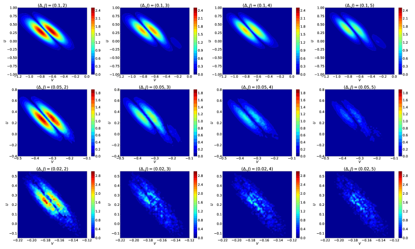
Figure 1: Heatmap of the absolute error for the CF-expansion in the case of the hypo-elliptic FHN model (see Section 4). Rows correspond to 3 choices $\displaystyle\Delta=(0.1,0.05,0.02)$ and columns to 4 choices $\displaystyle J=2,3,4,5$.

2 Closed-Form Transition Density Expansion

We will present a new CF transition density expansion for a wide class of Itô processes in (1.1), including the family of hypo-elliptic SDEs specified in (H). We write the transition density of $\displaystyle X_{t+\Delta}$ given $\displaystyle X_{t}=x\in\mathbb{R}^{N}$ as $\displaystyle y\mapsto p^{X}_{\Delta}(x,y;\theta):=\mathbb{P}(X_{t+\Delta}\in dy\,|\,X_{t}=x)/dy$, with $\displaystyle t\geq 0$, $\displaystyle\Delta>0$.

2.1 Conditions for Closed-Form Expansion

Assumption 1.

For both model classes (E) and (H), the maps $\displaystyle x\mapsto V_{j}(x,\theta)$, $\displaystyle 0\leq j\leq d$, are infinitely differentiable for any $\displaystyle\theta\in\Theta$.

For a vector-valued $\displaystyle V:\mathbb{R}^{N}\to\mathbb{R}^{N}$, we make use of the standard correspondence $\displaystyle V\leftrightarrow\textstyle\sum_{i=1}^{N}V^{i}\partial_{i}$.

Assumption 2.

We distinguish between model classes (E) and (H).

• For class (E), it holds that $\displaystyle a_{R}(x,\theta)=(\sigma_{R}\sigma_{R})^{\top}(x,\theta)$ is positive definite for all $\displaystyle(x,\theta)\in\mathbb{R}^{N}\times\Theta$. This is equivalent to $\displaystyle\mathrm{Span}\{V_{R,j}(x,\theta),\,1\leq j\leq d\}=\mathbb{R}^{N},$ for all $\displaystyle(x,\theta)\in\mathbb{R}^{N}\times\Theta$.

• For class (H), it holds that:

  $$\displaystyle\mathrm{Span}\bigl{\{}V_{R,j}(x,\theta),\,1\leq j\leq d\bigr{\}}=\mathbb{R}^{N_{R}},\qquad\mathrm{Span}\Bigl{\{}\bigl{\{}V_{j}(x,\theta),\,[\widetilde{V}_{0},V_{j}](x,\theta)\bigr{\}},\,1\leq j\leq d\Bigr{\}}=\mathbb{R}^{N},$$

  for all $\displaystyle(x,\theta)\in\mathbb{R}^{N}\times\Theta$, where $\displaystyle\widetilde{V}_{0}:\mathbb{R}^{N}\times\Theta\to\mathbb{R}^{N}$ is the drift function when the Itô SDE (H) is written in a Stratonovich form, namely $\displaystyle\textstyle\widetilde{V}_{0}(x,\theta)=V_{0}(x,\theta)-\tfrac{1}{2}\sum_{j=1}^{d}\sum_{i=1}^{N}V_{j}^{i}(x,\theta)\partial_{x_{i}}V_{j}(x,\theta).$

Assumption 2 is related to Hörmander’s condition (it suffices for Hörmander’s condition to hold) and implies that the law of $\displaystyle X_{t}$, $\displaystyle t>0$, admits a Lebesgue density. For the hypo-elliptic class (H), Assumption 2-II guarantees that the noise in the rough component $\displaystyle X_{R,t}$ (of size $\displaystyle\sqrt{t}$ for a period of length $\displaystyle t$) propagates into the smooth component $\displaystyle X_{S,t}$. Inclusion of the vector fields $\displaystyle[\widetilde{V}_{0},V_{j}](x,\theta)$, $\displaystyle 1\leq j\leq d$, relates to the appearance of terms $\displaystyle\textstyle\int_{0}^{t}B_{s}^{j}ds$ (of a different scale $\displaystyle\sqrt{t^{3}}$) in the smooth component $\displaystyle X_{S,t}$ after an Itô-Taylor expansion of $\displaystyle\textstyle\int_{0}^{t}V_{S,0}(X_{u},\theta)du$. Thus, the transition law of SDE (H) is non-degenerate and admits a Lebesgue density even if not all coordinates are directly driven by the Brownian motion. A precise definition of Hörmander’s condition can be found, e.g., in Nualart (2006).

2.2 Background Idea

Before presenting the CF-expansion we explain an idea that underpins its development – more precisely the starting point of the latter. Consider the elliptic class (E) and the Euler-Maruyama (EM) scheme which approximates the transition dynamics of $\displaystyle X_{t+\Delta}|X_{t}=x$, with $\displaystyle x\in\mathbb{R}^{N}$, $\displaystyle t>0$, $\displaystyle\Delta>0$, so that:

$$\displaystyle\bar{X}_{t+\Delta}^{\mathrm{EM},\theta}:=x+V_{R,0}(x,\theta)\Delta+\sigma_{R}(x,\theta)\bigl{(}B_{t+\Delta}-B_{t}\bigr{)}.$$ (2.1)

Under regularity conditions on $\displaystyle x\mapsto V_{R,j}(x,\theta)$, $\displaystyle 0\leq j\leq d$, and the requirement that the matrix $\displaystyle a_{R}(x,\theta)=(\sigma_{R}\sigma_{R}^{\top})(x,\theta)$ is positive definite for all $\displaystyle(x,\theta)\in\mathbb{R}^{N}\times\Theta$, the EM scheme gives rise to a well-defined baseline Gaussian transition density, $\displaystyle y\mapsto p_{\Delta}^{\bar{X}^{\mathrm{EM}}}(x,y;\theta)$. In the present elliptic setting Iguchi and Yamada (2021) constructed a CF transition density approximation of the following form:

$$\displaystyle p^{X}_{\Delta}(x,y;\theta)\approx p^{\bar{X}^{\mathrm{EM}}}_{\Delta}(x,y;\theta)\times\bigl{(}1+(\mathrm{correction\,term})\bigr{)}.$$ (2.2)

The tools utilised in Iguchi and Yamada (2021) to derive the approximation include Taylor expansion, Kolmogorov backward/forward equations, use of the infinitesimal generators for the target SDE and its EM approximation. In the above expression, the ‘correction term’ involves $\displaystyle\Delta$, partial derivatives of the SDE coefficients and Hermite polynomials obtained via differentiating the transition density of the EM scheme. As mentioned in the Introduction, other approaches are also available, including the ones developed in Aït-Sahalia (2002, 2008); Li (2013); Yang et al. (2019), and all such works also assume invertibility of the matrix $\displaystyle a_{R}$, thus are not relevant for the hypo-elliptic class (H).

To construct a CF transition density expansion for a broader family of SDEs that includes hypo-elliptic SDEs, it is critical to choose an appropriate reference Gaussian density which is non-degenerate for the target class of models. To achieve this, we consider the local drift linearisation (LDL) scheme, which, upon application on the general SDE model in (1.1), is defined via the following expression, for each given $\displaystyle t\geq 0$, $\displaystyle\Delta>0$, and for $\displaystyle\bar{X}_{t}^{\theta}=x\in\mathbb{R}^{N}$:

$$\displaystyle\bar{X}_{t+\Delta}^{\theta}=x+\int_{t}^{t+\Delta}\bigl{(}A_{x,\theta}\bar{X}_{s}^{\theta}+b_{x,\theta}\bigr{)}ds+\sigma(x,\theta)\bigl{(}B_{t+\Delta}-B_{t}\bigr{)},$$ (2.3)

where $\displaystyle A_{x,\theta}\in\mathbb{R}^{N\times N}$ and $\displaystyle b_{x,\theta}\in\mathbb{R}^{N}$ are specified as follows:

$$\displaystyle A_{x,\theta}=\bigl{[}\partial_{x_{j}}V_{0}^{i}(x,\theta)\bigr{]}_{1\leq i,j\leq N},\qquad b_{x,\theta}=V_{0}(x,\theta)-A_{x,\theta}\,x.$$

That is, (2.3) is obtained from a 1st-order Taylor expansion of the drift $\displaystyle V_{0}$ about the initial position $\displaystyle x$ and $\displaystyle\sigma(\cdot)$ fixed at its initial value. Expression (2.3) corresponds to a linear SDE, with a solution for $\displaystyle\bar{X}_{t+\Delta}^{\theta}|\bar{X}_{t}^{\theta}=x$ that has the following explicit form:

$$\displaystyle\bar{X}_{t+\Delta}^{\theta}=e^{\Delta A_{x,\theta}}x+\int_{t}^{t+\Delta}e^{(t+\Delta-s)A_{x,\theta}}b_{x,\theta}\,ds+\int_{t}^{t+\Delta}e^{(t+\Delta-s)A_{x,\theta}}\sigma(x,\theta)\,dB_{s}.$$

Thus, $\displaystyle\bar{X}_{t+\Delta}^{\theta}|\bar{X}_{t}^{\theta}=x$ follows a Gaussian law, with mean $\displaystyle\mu(\Delta,x,\theta)$ and covariance $\displaystyle\Sigma(\Delta,x,\theta)$ given as:

$$\displaystyle\mu(\Delta,x,\theta)=e^{\Delta A_{x,\theta}}\hat{\mu}^{x}(\Delta,x,\theta),\qquad\hat{\mu}^{z}(\Delta,x,\theta):=x+\int_{0}^{\Delta}e^{-sA_{z,\theta}}b_{z,\theta}ds,\quad z\in\mathbb{R}^{N};$$ (2.4)

$$\displaystyle\Sigma(\Delta,x,\theta)=e^{\Delta A_{x,\theta}}\hat{\Sigma}(\Delta,x,\theta)e^{\Delta A_{x,\theta}^{\top}},\qquad\hat{\Sigma}(\Delta,x,\theta):=\int_{0}^{\Delta}e^{-sA_{x,\theta}}a(x,\theta)e^{-sA_{x,\theta}^{\top}}ds.$$ (2.5)

The introduction of the extra argument $\displaystyle z$ in $\displaystyle\hat{\mu}^{z}(\Delta,x,\theta)$ will be of use in later developments.

In the sequel we show that $\displaystyle\hat{\Sigma}$ (thus also $\displaystyle\Sigma$) is positive definite for both model classes (E), (H) under Assumption 2. Then, under regularity conditions on the SDE coefficients together with the invertibility $\displaystyle\Sigma$, we appropriately expand upon the direction followed by Iguchi and Yamada (2021) to construct a CF transition density approximation that covers the model class (H) and writes as:

$$\displaystyle p^{X}_{\Delta}(x,y;\theta)\approx p^{\bar{X}}_{\Delta}(x,y;\theta)\times\bigl{(}1+(\mathrm{correction\,term})\bigr{)},$$ (2.6)

where $\displaystyle y\mapsto p^{\bar{X}}_{\Delta}(x,y;\theta)$ is the transition density of the LDL scheme (2.3). Similarly to the case of the expansion for elliptic diffusions, the correction term appearing in (2.6) involves partial derivatives of SDE coefficients w.r.t. the state argument and Hermite polynomials now defined via partial derivatives of the non-degenerate Gaussian density $\displaystyle p_{\Delta}^{\bar{X}}(x,y;\theta)$.

Remark 2.1.

Iguchi and Yamada (2021) work in an elliptic setting to develop Monte-Carlo estimators of improved weak order of convergence for $\displaystyle\mathbb{E}[\varphi(X_{T})]$, $\displaystyle\varphi:\mathbb{R}^{N}\to\mathbb{R}$, $\displaystyle T>0$, and their expansion in the form of (2.2) is used for such a purpose. In brief, they use samples from the baseline $\displaystyle p_{\Delta}^{\bar{X}^{\mathrm{EM}}}(x,y;\theta)$, weighted by $\displaystyle(1+(\mathrm{correction\,term}))$, in an iterative procedure over $\displaystyle\left\lfloor T/\Delta\right\rfloor$ steps. Even if the initial derivations in the CF-expansion we develop here resemble steps followed in Iguchi and Yamada (2021), our objectives and, consequently, the structure of the CF-expansion and its theoretical analysis (and, in general, the overall contribution) fully deviate from Iguchi and Yamada (2021).

2.3 Non-Degeneracy of the LDL Scheme

As mentioned in Section 2.2, existence of a Lebesgue density for the transition dynamics of the LDL scheme (2.3) is essential for the construction of our CF-expansion for both model classes (E) and (H). In this section we show that such an existence is implied by Assumption 2. That is, we show under Assumption 2, i.e. Hörmander’s condition for the target model classes (E) and (H), that the vector fields defined via the LDL scheme (2.3) also satisfy Hörmander’s condition. Specifically, the vector fields defined from the coefficients of (2.3) coincide with those of the original SDE, upon fixing the argument $\displaystyle x$ to the initial condition of (2.3). We thus have the following result whose proof is given in Appendix 6.1.

Lemma 2.1.

Let $\displaystyle(\Delta,x,\theta)\in(0,\infty)\times\mathbb{R}^{N}\times\Theta$. Under Assumptions 1-2, the law of $\displaystyle\bar{X}_{t+\Delta}^{\theta}|\bar{X}_{t}^{\theta}=x$ defined in (2.3) admits a smooth Lebesgue density for model classes (E) and (H).

We describe a sub-class from (H) where the LDL scheme delivers well-posed Lebesgue densities for SDE transition dynamics while the Euler-Maruyama scheme provides degenerate distributions.

Example 1 (Underdamped Langevin Equation).

We consider the following bivariate SDE:

$$\displaystyle\begin{aligned} dX_{t}^{1}&=X_{t}^{2}\,dt;\qquad dX_{t}^{2}&=\bigl{(}-V^{\prime}(X_{t}^{1})-\alpha X_{t}^{2}\bigr{)}dt+\sigma\,dB_{1,t},\end{aligned}$$ (2.7)

for parameters $\displaystyle\alpha,\sigma>0$ and potential $\displaystyle V:\mathbb{R}\to\mathbb{R}$. Such dynamics are used to describe the motion of a particle on the real line $\displaystyle\mathbb{R}$, with $\displaystyle X_{t}^{1}$ and $\displaystyle X_{t}^{2}$ representing position and momentum, respectively. The coefficients in SDE (2.7) correspond to the following vector fields, for $\displaystyle x=(x_{1},x_{2})\in\mathbb{R}^{2}$:

$$\displaystyle V_{0}\equiv\widetilde{V}_{0}=x_{2}\partial_{x_{1}}+\bigl{(}-V^{\prime}(x_{1})-\alpha x_{2}\bigr{)}\partial_{x_{2}},\qquad V_{1}=\sigma\partial_{x_{2}}.$$

The diffusion matrix is degenerate, so (2.7) belongs to class (H). Also, Assumption 2-II is satisfied as:

$$\displaystyle V_{1}(x)=[0,\sigma]^{\top},\qquad[\widetilde{V}_{0},V_{1}](x)=\widetilde{V}_{0}V_{1}(x)-V_{1}\widetilde{V}_{0}(x)=[-\sigma,\sigma\alpha]^{\top},$$ (2.8)

and, given $\displaystyle\sigma,\alpha>0$, we get that $\displaystyle\mathrm{Span}\{V_{1}(x),[V_{0},V_{1}](x)\}=\mathbb{R}^{2},$ for all $\displaystyle x\in\mathbb{R}^{2}$. The Euler-Maruyama scheme for $\displaystyle\bar{X}_{t+\Delta}^{\mathrm{EM}}|\bar{X}_{t}^{\mathrm{EM}}=x$ writes as:

$$\displaystyle\bar{X}_{t+\Delta}^{\mathrm{EM},1}=x_{1}+x_{2}\Delta;\qquad\bar{X}_{t+\Delta}^{\mathrm{EM},2}=x_{2}+\bigl{(}-V^{\prime}(x_{1})-\alpha x_{2}\bigr{)}\Delta+\sigma(B_{1,t+\Delta}-B_{1,t}).$$ (2.9)

So, the law of $\displaystyle\bar{X}_{t+\Delta}^{\mathrm{EM}}|\bar{X}_{t}^{\mathrm{EM}}$ involves a degenerate covariance matrix. In contrast, in this setting the LDL scheme (2.3) contains the $\displaystyle 2\times 2$ matrix $\displaystyle A_{x}$ and the vector $\displaystyle b_{x}$ specified as follows:

$$\displaystyle[A_{x}]_{11}=0,\ \ [A_{x}]_{12}=1,\ \ [A_{x}]_{21}=-V^{\prime\prime}(x_{1}),\ \ [A_{x}]_{22}=-\alpha,\quad b^{1}_{x}=0,\ \ b^{2}_{x}=-V^{\prime}(x_{1})+V^{\prime\prime}(x_{1})x_{1}.$$

The vector fields associated with the coefficients of the LDL scheme are given as follows, for $\displaystyle x,z\in\mathbb{R}^{2}$:

$$\displaystyle\bar{V}_{0}^{z}=\sum_{i=1,2}[A_{z}x+b_{z}]_{i}\partial_{x_{i}},\qquad\bar{V}_{1}=\sigma\partial_{x_{2}},$$

where (with some abuse of notation) we introduce $\displaystyle z\in\mathbb{R}^{2}$ to represent the initial condition for (2.3), thus distinguish the latter from argument $\displaystyle x\in\mathbb{R}^{2}$ upon which the linear drift in (2.3) applies. For the above vector fields, Hörmander’s condition holds via:

$$\displaystyle\bar{V}_{1}(x)=\bigl{[}0,\sigma]^{\top},\qquad[\bar{V}_{0}^{z},\bar{V}_{1}](x)=-\bar{V}_{1}\bar{V}_{0}^{z}(x)=\bigl{[}-\sigma,\sigma\alpha\bigr{]}^{\top}.$$ (2.10)

Thus, the law of $\displaystyle\bar{X}_{t+\Delta}|\bar{X}_{t}$ admits a well-defined (Gaussian) transition density. Note that the vector fields in (2.10) coincide with the ones in (2.8) defined for the original SDE (2.7), so the hypo-ellipticity of the target SDE is inherited by its induced LDL scheme.

2.4 Transition Density CF Expansion

2.4.1 Preliminaries

We prepare some ingredients for the construction of our CF-expansion. We define the LDL scheme starting from a point $\displaystyle x\in\mathbb{R}^{N}$ with its coefficients being frozen at a point $\displaystyle z\in\mathbb{R}^{N}$ as:

$$\displaystyle d\bar{X}_{t}^{\theta,z}=\bigl{(}A_{z,\theta}\bar{X}_{t}^{\theta,z}+b_{z,\theta}\bigr{)}dt+\sigma(z,\theta)dB_{t},\qquad\bar{X}_{0}^{\theta,z}=x_{0}\in\mathbb{R}^{N}.$$ (2.11)

Notice that $\displaystyle\big{[}\,\bar{X}_{t}^{\theta,z}|_{z=x}\,\big{|}\,\bar{X}_{0}^{\theta,z}=x\,\big{]}\equiv[\bar{X}_{t}^{\theta}|\bar{X}_{0}^{\theta}=x]$. The generator corresponding to (2.11) is given as:

$$\displaystyle\mathscr{L}_{\theta}^{0,z}\varphi(x) \displaystyle=\sum_{1\leq i\leq N}\bigl{[}A_{z,\theta}x+b_{z,\theta}\bigr{]}_{i}\partial_{i}\varphi(x)+\tfrac{1}{2}\sum_{1\leq i_{1},i_{2}\leq N}\sum_{1\leq j\leq d}V_{j}^{i_{1}}(z,\theta)V_{j}^{i_{2}}(z,\theta)\partial_{i_{1}i_{2}}\varphi(x),$$

for $\displaystyle\varphi:\mathbb{R}^{N}\to\mathbb{R}$, $\displaystyle x,z\in\mathbb{R}^{N}$, $\displaystyle\theta\in\Theta$. Notice that $\displaystyle\bar{X}^{\theta,z}_{t+\Delta}|\bar{X}_{t}^{\theta,z}=x\sim\mathscr{N}\big{(}e^{\Delta A_{z,\theta}}\hat{\mu}^{z}(\Delta,x,\theta),\Sigma(\Delta,z,\theta)\big{)}$, where $\displaystyle\hat{\mu}^{z}$ and $\displaystyle\Sigma$ are defined in (2.4) and (2.5), respectively. We write the density of $\displaystyle\bar{X}^{\theta,z}_{t+\Delta}|\bar{X}_{t}^{\theta,z}=x$ as $\displaystyle y\mapsto p^{\bar{X}^{z}}_{\Delta}(x,y;\theta)$ and note that $\displaystyle p^{\bar{X}^{z}}_{\Delta}(x,y;\theta)|_{z=x}\equiv p^{\bar{X}}_{\Delta}(x,y;\theta)$, where the right-hand-side is the transition density of the LDL scheme (2.3).

We introduce semi-groups $\displaystyle\{P_{t}^{\theta}\}_{t\geq 0}$ and $\displaystyle\{\bar{P}_{t}^{\theta,z}\}_{t\geq 0}$ associated with the Markov processes $\displaystyle\{X_{t}\}_{t\geq 0}$ and $\displaystyle\{\bar{X}_{t}^{\theta,z}\}_{t\geq 0}$, respectively as follows:

$$\displaystyle P_{t}^{\theta}\varphi(x)=\int_{\mathbb{R}^{N}}\varphi(y)p^{X}_{t}(x,y;\theta)dy,\qquad\bar{P}_{t}^{\theta,z}\varphi(x)=\int_{\mathbb{R}^{N}}\varphi(y)p^{\bar{X}^{z}}_{t}(x,y;\theta)dy,\quad z\in\mathbb{R}^{N},$$ (2.12)

for $\displaystyle\varphi:\mathbb{R}^{N}\to\mathbb{R}$ and $\displaystyle(t,x,\theta)\in(0,\infty)\times\mathbb{R}^{N}\times\Theta$. For notational simplicity, we introduce:

$$\displaystyle\widetilde{\mathscr{L}}^{z}_{\theta}:=\mathscr{L}_{\theta}-\mathscr{L}_{\theta}^{0,z},$$ (2.13)

where we recall that $\displaystyle\mathscr{L}_{\theta}$ is the generator associated with the target SDE, given in (1.4). The first steps in the derivation of our CF-expansion are provided in the following two results.

Lemma 2.2.

Let $\displaystyle t>0$, $\displaystyle x,y\in\mathbb{R}^{N}$ and $\displaystyle\theta\in\Theta$. Also, let $\displaystyle\varphi\in C^{\infty}(\mathbb{R}^{N};\mathbb{R})$. It holds that:

$$\displaystyle p^{X}_{t}(x,y;\theta) \displaystyle=p^{\bar{X}^{z}}_{t}(x,y;\theta)|_{z=x}+\int_{0}^{t}P_{s}^{\theta}\widetilde{\mathscr{L}}_{\theta}^{z}p^{\bar{X}^{z}}_{t-s}(\cdot,y;\theta)(x)|_{z=x}ds;$$ (2.14)

$$\displaystyle P_{t}^{\theta}\varphi(x) \displaystyle=\bar{P}_{t}^{\theta,z}\varphi(x)|_{z=x}+\int_{0}^{t}P_{s}^{\theta}\widetilde{\mathscr{L}}^{z}_{\theta}\bar{P}_{t-s}^{\theta,z}\varphi(x)|_{z=x}ds.$$ (2.15)

Lemma 2.3.

Let $\displaystyle 0<s<t$, $\displaystyle\theta\in\Theta$ and $\displaystyle z,x,y\in\mathbb{R}^{N}$. Then it holds that, for any $\displaystyle K\in\mathbb{N}$,

$$\displaystyle\bar{P}_{s}^{\theta,z}\widetilde{\mathscr{L}}_{\theta}^{z}\bar{P}_{t-s}^{\theta,z}\varphi(x) \displaystyle=\sum_{0\leq k\leq K}\frac{s^{k}}{k!}\bigl{\{}\mathrm{ad}^{k}_{\mathscr{L}_{\theta}^{0,z}}(\widetilde{\mathscr{L}}_{\theta}^{z})\bigr{\}}\bar{P}_{t}^{\theta,z}\varphi(x)+\mathscr{R}^{K+1,z}(s,t,x;\theta);$$ (2.16)

$$\displaystyle\bar{P}_{s}^{\theta,z}\widetilde{\mathscr{L}}_{\theta}^{z}p^{\bar{X}^{z}}_{t-s}(\cdot,y;\theta)(x) \displaystyle=\sum_{0\leq k\leq K}\frac{s^{k}}{k!}\bigl{\{}\mathrm{ad}^{k}_{\mathscr{L}_{\theta}^{0,z}}(\widetilde{\mathscr{L}}_{\theta}^{z})\bigr{\}}\{p^{\bar{X}^{z}}_{t}(\cdot,y;\theta)\}(x)+\widetilde{\mathscr{R}}^{K+1,z}(s,t,x,y;\theta)$$ (2.17)

where the remainder terms $\displaystyle{\mathscr{R}}^{K+1,z}$ and $\displaystyle\widetilde{\mathscr{R}}^{K+1,z}$ are specified in the proof of Lemma 2.3 in Appendix 6.

Results similar to the above, for the elliptic case and for the Euler-Maruyama scheme used as a baseline transition density, are obtained in Iguchi and Yamada (2021).

2.4.2 Construction of CF-Expansion

Based on the auxiliary results (Lemma 2.1, 2.2 and 2.3) in the previous subsections, we construct a CF transition density expansion in the following three steps:

Step 1. We recursively apply formula (2.15) within (2.14), from Lemma 2.2, to obtain for any $\displaystyle M\in\mathbb{N}$:

$$\displaystyle p^{X}_{\Delta}(x,y;\theta) \displaystyle=p^{\bar{X}^{z}}_{\Delta}(x,y;\theta)|_{z=x}+\int_{0}^{\Delta}{P}_{s_{1}}^{\theta}\widetilde{\mathscr{L}}_{\theta}^{z}p_{\Delta-s_{1}}^{\bar{X}^{z}}(\cdot,y;\theta)(x)|_{z=x}ds_{1}$$

$$\displaystyle=p^{\bar{X}^{x}}_{\Delta}(x,y;\theta)+\sum_{1\leq j\leq M-1}\mathscr{T}^{j}(\Delta,x,y;\theta)\ \ +\ \ \mathscr{R}_{1}^{M}(\Delta,x,y;\theta),$$ (2.18)

where we have set:

$$\displaystyle\mathscr{T}^{\,j}(\Delta,x,y;\theta)=\int_{I(s_{1:j})}\bar{P}_{s_{j}}^{\theta,z}\widetilde{\mathscr{L}}_{\theta}^{z}\bar{P}_{s_{j-1}-s_{j}}^{\theta,z}\cdots\widetilde{\mathscr{L}}_{\theta}^{z}\bar{P}_{s_{1}-s_{2}}^{\theta,z}\widetilde{\mathscr{L}}_{\theta}^{z}p_{\Delta-s_{1}}^{\bar{X}^{z}}(\cdot,y;\theta)(x)\big{|}_{z=x}\,ds_{j}\cdots ds_{1};$$

$$\displaystyle\mathscr{R}_{1}^{M}(\Delta,x,y;\theta)=\int_{I(s_{1:M})}{P}_{s_{M}}^{\theta}\widetilde{\mathscr{L}}_{\theta}^{z}\bar{P}_{s_{M-1}-s_{M}}^{\theta,z}\cdots\widetilde{\mathscr{L}}_{\theta}^{z}\bar{P}_{s_{1}-s_{2}}^{\theta,z}\widetilde{\mathscr{L}}_{\theta}^{z}p_{\Delta-s_{1}}^{\bar{X}^{z}}(\cdot,y;\theta)(x)\big{|}_{z=x}\,ds_{M}\cdots ds_{1},$$ (2.19)

$$\displaystyle\qquad\qquad\qquad\quad I(s_{1:k}):=\{s_{1:k}=(s_{1},\ldots,s_{k}):0\leq s_{k}\leq\cdots\leq s_{1}\leq\Delta\},\quad k\geq 0,$$

with the convention $\displaystyle s_{0}\equiv\Delta$.

Step 2. Since $\displaystyle\mathscr{T}^{j}(\Delta,x,y;\theta)$, $\displaystyle 1\leq j\leq M$, is not tractable, we obtain a computable quantity for it via use of Lemma 2.3. Let $\displaystyle\mathscr{T}_{s_{1:j}}(\Delta,x,y;\theta)$ be the integrand of $\displaystyle\mathscr{T}^{j}(\Delta,x,y;\theta)$, so that $\displaystyle\mathscr{T}^{j}(\Delta,x,y;\theta)=\textstyle\int_{I(s_{1:j})}\mathscr{T}_{s_{1:j}}(\Delta,x,y;\theta)ds_{j}\cdots ds_{1}$. Recursive application of Lemma 2.3 to $\displaystyle\mathscr{T}_{s_{1:j}}$, $\displaystyle 1\leq j\leq M-1$, gives:

$$\displaystyle\mathscr{T}_{s_{1:j}}(\Delta,x,y;\theta)=\sum_{\begin{subarray}{c}\alpha\leq\beta^{[j]}\end{subarray}}\frac{\prod_{k=1}^{j}(s_{k})^{\alpha_{k}}}{\alpha!}\cdot\mathscr{D}_{\alpha}^{z,\theta}\bigl{\{}p^{\bar{X}^{z}}_{\Delta}(\cdot,y;\theta)\bigr{\}}(x)\bigr{|}_{z=x}+\mathscr{E}^{\beta^{[j]}}_{s_{1:j}}(\Delta,x,y;\theta),$$ (2.20)

for a multi-index $\displaystyle\beta^{[j]}=(\beta_{1}^{[j]},\ldots,\beta_{j}^{[j]})\in\mathbb{Z}_{\geq 0}^{j}$, where we have defined:

$$\displaystyle\mathscr{D}_{\alpha}^{z,\theta} \displaystyle\equiv\Bigl{(}\mathrm{ad}_{\mathscr{L}_{\theta}^{0,z}}^{\alpha_{j}}(\widetilde{\mathscr{L}}_{\theta}^{z})\Bigr{)}\Bigl{(}\mathrm{ad}_{\mathscr{L}_{\theta}^{0,z}}^{\alpha_{j-1}}(\widetilde{\mathscr{L}}_{\theta}^{z})\Bigr{)}\cdots\Bigl{(}\mathrm{ad}_{\mathscr{L}_{\theta}^{0,z}}^{\alpha_{1}}(\widetilde{\mathscr{L}}_{\theta}^{z})\Bigr{)},\qquad z\in\mathbb{R}^{N},\,\theta\in\Theta,$$ (2.21)

and the residual $\displaystyle\mathscr{E}^{\beta^{[j]}}_{s_{1:j}}(\Delta,x,y;\theta)$ is given in (7.54) in Appendix 7.5. We now obtain, for $\displaystyle 1\leq j\leq M-1$:

$$\displaystyle\mathscr{T}^{j}(\Delta,x,y;\theta)=\sum_{\begin{subarray}{c}\alpha\leq\beta^{[j]}\end{subarray}}\Delta^{|\alpha|+j}\cdot\tfrac{K(\alpha)}{\alpha!}\cdot\mathscr{D}_{\alpha}^{z,\theta}\{p^{\bar{X}^{z}}_{\Delta}(\cdot,y;\theta)\}(x)|_{z=x}+\mathscr{R}_{2}^{\,j,\beta^{[j]}}(\Delta,x,y,\theta),$$ (2.22)

$$\displaystyle\qquad\qquad\qquad K(\alpha):=\int_{0\leq s_{j}\leq\cdots\leq s_{1}\leq 1}\prod_{1\leq k\leq j}(s_{k})^{\alpha_{k}}ds_{j}\cdots ds_{1},$$

$$\displaystyle\qquad\qquad\qquad\mathscr{R}_{2}^{\,j,\beta^{[j]}}(\Delta,x,y,\theta):=\int_{I(s_{1:j})}\mathscr{E}^{\beta^{[j]}}_{s_{1:j}}(\Delta,x,y;\theta)ds_{j}\cdots ds_{1}.$$ (2.23)

Step 3. From (2.18) in Step 1. and (2.22) in Step 2., we obtain the following CF-expansion for the true (intractable) transition density. For any $\displaystyle M\geq 1$ and multi-indices $\displaystyle\beta^{[j]}\in\mathbb{Z}_{\geq 0}^{j}$, $\displaystyle 1\leq j\leq M-1$:

$$\displaystyle p^{X}_{\Delta}(x,y;\theta) \displaystyle=p^{\bar{X}}_{\Delta}(x,y;\theta)+\sum_{1\leq j\leq M-1}\sum_{\begin{subarray}{c}\alpha\leq\beta^{[j]}\end{subarray}}\Delta^{|\alpha|+j}\cdot\tfrac{K(\alpha)}{\alpha!}\cdot\mathscr{D}_{\alpha}^{z,\theta}\{p^{\bar{X}^{z}}_{\Delta}(\cdot,y;\theta)\}(x)\Bigr{|}_{z=x}$$

$$\displaystyle\qquad\qquad\qquad\qquad\qquad+\mathscr{R}_{1}^{M}(\Delta,x,y;\theta)+\sum_{1\leq j\leq M-1}\mathscr{R}_{2}^{\,j,\beta^{[j]}}(\Delta,x,y,\theta),$$ (2.24)

where $\displaystyle\mathscr{R}_{1}^{M}$, $\displaystyle\mathscr{R}_{2}^{\,j,\beta^{[j]}}$ are defined in (2.19), (2.23), respectively. Under assumptions, we show in Section 3.1 that the remainder terms are of size $\displaystyle\mathcal{O}(\Delta^{p})$ for an arbitrary $\displaystyle p>0$ by choosing a large enough $\displaystyle M$ and appropriate $\displaystyle\beta^{[j]}$, $\displaystyle 1\leq j\leq M-1$. The double sum in (2.24) involves tractable terms and can be utilised as a proxy for the true transition density. In particular, the expansion is well-defined for both model classes (E) and (H) since the Gaussian density $\displaystyle p^{\bar{X}^{z}}(x,y;\theta)$ and its partial derivatives (involved in $\displaystyle\mathscr{D}_{\alpha}^{z,\theta}\bigl{\{}p_{\Delta}^{\bar{X}^{z}}(\cdot,y;\theta)(x)\bigr{\}}|_{z=x}$) are well-defined from Lemma 2.1. We note that the tractable double sum in (2.24) is regarded as a CF-expansion, but the current form of the expansion does not yet correspond to the ‘$\displaystyle\Delta$’-expansion (1.3). For instance, the exponents of the step-size $\displaystyle\Delta$ are integers in (2.24), while they are given as $\displaystyle k/2$, $\displaystyle k\in\mathbb{N}$, in (1.3). However, we emphasise that (2.24) will be ultimately expressed as a $\displaystyle\Delta$-expansion of the form in (1.3) after carefully working with the terms $\displaystyle\mathscr{D}_{\alpha}^{z,\theta}\{p^{\bar{X}^{z}}_{\Delta}(\cdot,y;\theta)\}(x)$. Indeed, taking partial derivatives of $\displaystyle x\mapsto p^{\bar{X}^{z}}(x,y;\theta)$, will give Hermite polynomials and powers $\displaystyle\Delta^{-k/2}$, where the integer $\displaystyle k$ depends on the number of derivatives. We explain this in detail later on in Section 3.2.

3 Error Analysis for the CF-Expansion

In Section 2.4 we have constructed a CF-expansion (2.24) for the true transition density. Our objective now is to provide rigorous error estimates for this expansion, thus theoretically justifying its derivation, similarly to results obtained by a few earlier works in the case of the elliptic class (E). We also describe that the obtained expansion (3.4) can be given in the form (1.3), namely a series in powers of $\displaystyle\Delta$. As the error estimates vary for classes (E), (H), we make use of the notation $\displaystyle w\in\{\ref{eq:ellip},\ref{eq:hypo}\}$ and write $\displaystyle p^{X,(w)}\equiv p^{X}$, $\displaystyle p^{\bar{X},(w)}\equiv p^{\bar{X}}$, $\displaystyle\mathscr{R}_{1}^{M,(w)}\equiv\mathscr{R}_{1}^{M}$ and $\displaystyle\mathscr{R}_{2}^{\,j,\beta^{[j]},(w)}\equiv\mathscr{R}_{2}^{\,j,\beta^{[j]}}$ to indicate the class under consideration.

3.1 Main Result

We derive upper bounds for the residuals of the CF expansion $\displaystyle\mathscr{R}_{1}^{M}$ and $\displaystyle\mathscr{R}_{2}^{j,\beta^{[j]}}$ specified in (2.19) and (2.23), respectively. We will need the following additional assumptions.

Assumption 3.

The parameter space $\displaystyle\Theta$ is compact. Also, for each $\displaystyle x\in\mathbb{R}^{N}$, the function $\displaystyle\theta\mapsto V_{j}(x,\theta)$ is continuous, $\displaystyle 0\leq j\leq d$.

Assumption 4.

Let $\displaystyle x\in\mathbb{R}^{N}$ be the initial state of the transition dynamics. The SDE coefficients satisfy the following properties:

• (Boundedness of drift at initial state): There exists a constant $\displaystyle\kappa>0$ such that $\displaystyle|x|+|V_{0}(x,\theta)|\leq\kappa$ for all $\displaystyle\theta\in\Theta$;

• (Uniform boundedness of diffusion coefficients): There exists a constant $\displaystyle C>0$ such that $\displaystyle|V_{j}(y,\theta)|\leq C$, $\displaystyle 1\leq j\leq d$, for all $\displaystyle(y,\theta)\in\mathbb{R}^{N}\times\Theta$;

• (Uniform boundedness of derivatives): There is a constant $\displaystyle C>0$ such that $\displaystyle\textstyle\sum_{j=0}^{d}|\partial^{\alpha}_{y}V_{j}(y,\theta)|\leq C$ for all $\displaystyle\alpha\in\mathbb{Z}^{N}_{\geq 0}$ with $\displaystyle|\alpha|\geq 1$ and all $\displaystyle(y,\theta)\in\mathbb{R}^{N}\times\Theta$.

Assumption 5.

For the hypo-elliptic model class (H), $\displaystyle N_{S}=N_{R}=d$.

Assumptions 3–5 suffice for obtaining appropriate bounds for the residuals of the CF-expansion. The uniform boundedness for the derivatives of the SDE coefficients is a standard assumption for the existence of a smooth transition density, when combined with Hörmander’s condition. Such uniform boundedness is also assumed in Li (2013) to control the residual of the expansion developed therein for elliptic SDEs. Assumptions 4–5 are used mainly in the proof of Theorem 1, where we need a upper bound for the true density $\displaystyle y\mapsto p^{X}_{\Delta}(x,y;\theta)$. Pigato (2022) shows that under Assumptions 4–5 the true transition density has a Gaussian-type bound as given later at (3.3). Based on this result, we show that the errors are appropriately bounded, analogously to Yang et al. (2019) who also used a Gaussian-type bound for the true density to control the residuals of an expansion for inhomogeneous elliptic SDEs. We stress that Assumptions 3–5 are not necessary for the construction of the CF-expansion, in the sense that our formulae can still be evaluated for SDEs with coefficients whose partial derivatives exhibit, e.g., polynomial growth as assumed in earlier works (Aït-Sahalia, 2008; Yang et al., 2019) for elliptic SDEs. The relaxation of our conditions is left for future research.

To provide a statement of our main result, we introduce some notation. We set:

$$\displaystyle m(\mathrm{\ref{eq:ellip}}):=N,\qquad m(\mathrm{\ref{eq:hypo}}):=4d.$$ (3.1)

Also, $\displaystyle\mathscr{G}^{(w)}:(0,\infty)\times\mathbb{R}^{N}\times\mathbb{R}^{N}\times\Theta\to\mathbb{R}$, $\displaystyle w\in\{\ref{eq:ellip},\ref{eq:hypo}\}$, is a mapping characterised as follows. There exist constants $\displaystyle C,c>0$ such that:

$$\displaystyle\bigl{|}\mathscr{G}^{(\ref{eq:ellip})}(t,x,y,\theta)\bigr{|} \displaystyle\leq Ct^{-\tfrac{m(\ref{eq:ellip})}{2}}\times\exp\Bigl{(}-c\tfrac{|y-x|^{2}}{t}\Bigr{)};$$ (3.2)

$$\displaystyle\bigl{|}\mathscr{G}^{(\ref{eq:hypo})}(t,x,y,\theta)\bigr{|} \displaystyle\leq Ct^{-\tfrac{m(\ref{eq:hypo})}{2}}\times\exp\left(-c\Bigl{(}\tfrac{|y_{S}-x_{S}-V_{S,0}(x,\theta)t|^{2}}{t^{3}}+\tfrac{|y_{R}-x_{R}|^{2}}{t}\Bigr{)}\right),$$ (3.3)

for all $\displaystyle(t,x,y,\theta)\in(0,\infty)\times\mathbb{R}^{N}\times\mathbb{R}^{N}\times\Theta$. Notice that for some constant $\displaystyle C>0$, for $\displaystyle\Delta\in(0,1)$:

$$\displaystyle\sup_{(x,y,\theta)\in\mathbb{R}^{N}\times\mathbb{R}^{N}\times\Theta}\bigl{|}\mathscr{G}^{(w)}(\Delta,x,y,\theta)\bigr{|}\leq C\Delta^{-\tfrac{m(w)}{2}},\qquad w\in\{\ref{eq:ellip},\ref{eq:hypo}\},$$

Theorem 1 (Bound for $\displaystyle\mathscr{R}_{1}^{M,(w)}$).

Let $\displaystyle x\in\mathbb{R}^{N}$ be the initial state of the transition dynamics and $\displaystyle M\geq 1$. Under Assumptions 1–5, there exist constants $\displaystyle C_{1},C_{2}>0$ such that for all $\displaystyle(\Delta,y,\theta)\in(0,1)\times\mathbb{R}^{N}\times\Theta$:

$$\displaystyle\bigl{|}\mathscr{R}_{1}^{M,(w)}(\Delta,x,y;\theta)\bigr{|}\leq C_{1}\Delta^{\tfrac{M}{2}}\times\bigl{|}\mathscr{G}^{(w)}(\Delta,x,y,\theta)\bigr{|}\leq C_{2}\Delta^{\tfrac{M-m(w)}{2}},\qquad w\in\{\ref{eq:ellip},\ref{eq:hypo}\}.$$

Theorem 2 (Bound for $\displaystyle\mathscr{R}_{2}^{\,j,\beta^{[j]},(w)}$).

Let $\displaystyle x\in\mathbb{R}^{N}$ be the initial state of the transition dynamics, and let $\displaystyle 1\leq j\leq M-1,\,M\in\mathbb{N}$, $\displaystyle\beta^{[j]}=(\beta^{[j]}_{1},\ldots,\beta^{[j]}_{j})\in\mathbb{Z}_{\geq 0}^{j}$. Under Assumptions 1–5, there exist constants $\displaystyle C_{1},C_{2}>0$ such that for all $\displaystyle(\Delta,y,\theta)\in(0,1)\times\mathbb{R}^{N}\times\Theta$:

$$\displaystyle\bigl{|}\mathscr{R}_{2}^{\,j,\beta^{[j]},(w)}(\Delta,x,y;\theta)\bigr{|}\leq C_{1}\Delta^{K^{[j],w}(\beta^{[j]})}\times\bigl{|}\mathscr{G}^{(w)}(\Delta,x,y,\theta)\bigr{|}\leq C_{2}\Delta^{K^{[j],w}(\beta^{[j]})-\tfrac{m(w)}{2}},\qquad w\in\{\ref{eq:ellip},\ref{eq:hypo}\},$$

$$\displaystyle\qquad\qquad\qquad K^{[j],\ref{eq:ellip}}(\beta^{[j]}):=\min_{1\leq i\leq j}\tfrac{\beta_{i}^{[j]}}{2}+\tfrac{j}{2},\qquad K^{[j],\mathrm{\ref{eq:hypo}}}(\beta^{[j]}):=\min_{1\leq i\leq j}\tfrac{1}{2}\bigl{(}\lfloor\tfrac{\beta_{i}^{[j]}}{2}\rfloor-\mathbf{1}_{\beta_{i}^{[j]}\geq 2}\bigr{)}+\tfrac{j}{2}.$$

The proofs of Theorems 1–2 are given in Appendix 7. From Theorem 2, by selecting the multi-index $\displaystyle\beta^{[j],(w)}\in\mathbb{Z}_{\geq 0}^{j}$ so that $\displaystyle K^{[j],w}(\beta^{[j],(w)})\geq\tfrac{M}{2}$, the residual $\displaystyle\mathscr{R}_{2}^{\,j,\beta^{[j]},(w)}$ becomes of size $\displaystyle\textstyle\mathcal{O}(\Delta^{\tfrac{M-m(w)}{2}})$, $\displaystyle w\in\{\ref{eq:ellip},\ref{eq:hypo}\}$. Thus, with this choice of $\displaystyle\beta^{[j],(w)}$, the residuals of the CF-expansion are controlled by $\displaystyle\mathcal{O}(\Delta^{\tfrac{M-m(w)}{2}})$, with $\displaystyle\Delta\in(0,1)$, $\displaystyle w\in\{\ref{eq:ellip},\ref{eq:hypo}\}$, and we can write:

$$\displaystyle\begin{aligned} p^{X,(w)}_{\Delta}(x,y;\theta)&={p^{\bar{X},(w)}_{\Delta}(x,y;\theta)+\sum_{1\leq j\leq M-1}\sum_{\begin{subarray}{c}\alpha\leq\beta^{[j],(w)}\end{subarray}}\Delta^{|\alpha|+j}\cdot\tfrac{K(\alpha)}{\alpha!}\cdot\mathscr{D}_{\alpha}^{z,\theta}\{p^{\bar{X}^{z},(w)}_{\Delta}(\cdot,y;\theta)\}(x)\Bigr{|}_{z=x}}\\ &\qquad\qquad\qquad\qquad\qquad\qquad\qquad\qquad\qquad\qquad\qquad\qquad\qquad+\mathcal{O}\bigl{(}\Delta^{\tfrac{M-m(w)}{2}}\bigr{)}.\end{aligned}$$ (3.4)

3.2 Series Expansion in $\displaystyle\Delta$

We study the CF-expansion given in (3.4) in detail. Expression (3.4) involves $\displaystyle\Delta^{|\alpha|+j}$ in front of each summand, but an additional $\displaystyle\Delta^{-K_{\alpha}/2}$, for some $\displaystyle K_{\alpha}\in\mathbb{N}$, is produced from $\displaystyle\mathscr{D}_{\alpha}^{z,\theta}\{p^{\bar{X}^{z}}_{\Delta}(\cdot,y;\theta)\}(x)$, where we recall that $\displaystyle\mathscr{D}_{\alpha}^{z,\theta}$ is the differential operator defined in (2.21). We show that upon rearrangement of terms in powers of $\displaystyle\Delta$, the right-hand-side of (3.4) attains the form of the $\displaystyle\Delta$-expansion in (1.3), i.e. a series expansion in (positive) powers of $\displaystyle\sqrt{\Delta}$. In particular, we clarify below that differentiating the Gaussian density $\displaystyle p^{\bar{X}^{z}}(x,y;\theta)$ w.r.t. the initial state $\displaystyle x\in\mathbb{R}^{N}$ produces additional powers $\displaystyle\Delta^{-{K}/{2}}$, for $\displaystyle K\geq 1$ depending on the number of derivatives. For the model class (H), the value of $\displaystyle K$ varies depending on whether the differentiation acts on smooth or rough components. We define, for $\displaystyle\alpha\in\mathbb{Z}_{\geq 0}^{N}$:

$$\displaystyle\|\alpha\|_{\ref{eq:ellip}}:=\tfrac{1}{2}|\alpha|,\qquad\|\alpha\|_{\ref{eq:hypo}}=\tfrac{3}{2}|\alpha_{S}|+\tfrac{1}{2}|\alpha_{R}|,$$ (3.5)

where, for class (H), we interpret $\displaystyle\alpha=(\alpha_{S,1},\ldots,\alpha_{S,N_{S}},\alpha_{R,1},\ldots,\alpha_{R,N_{R}})$ for given $\displaystyle\alpha_{S}\in\mathbb{Z}_{\geq 0}^{N_{S}}$, $\displaystyle\alpha_{R}\in\mathbb{Z}_{\geq 0}^{N_{R}}$. We then have the following key result whose proof is provided in Appendix 7.2:

Lemma 3.1.

Let $\displaystyle x,y\in\mathbb{R}^{N}$, $\displaystyle\theta\in\Theta$, $\displaystyle\Delta>0$. Also, let $\displaystyle\alpha\in\mathbb{Z}_{\geq 0}^{N}$. Under Assumptions 1–5, we have that:

$$\displaystyle\partial^{\alpha}_{x}\,p_{\Delta}^{\bar{X}^{z},(w)}(x,y;\theta)|_{z=x} \displaystyle=\Delta^{-\|\alpha\|_{w}}\times\mathscr{H}^{(w)}_{\alpha}(\Delta,x,y;\theta)\,p_{\Delta}^{\bar{X},(w)}(x,y;\theta),\qquad w\in\{\ref{eq:ellip},\ref{eq:hypo}\},$$

where $\displaystyle y\mapsto\mathscr{H}^{(w)}_{\alpha}(\Delta,x,y;\theta)$ is obtained explicitly defined via differentiation of $\displaystyle x\mapsto p_{\Delta}^{\bar{X}^{z},(w)}(x,y;\theta)$ and is characterised as follows. There exists a constant $\displaystyle C>0$ such that for all $\displaystyle\Delta>0$, $\displaystyle x,y\in\mathbb{R}^{N}$, $\displaystyle\theta\in\Theta$:

$$\displaystyle\bigl{|}\mathscr{H}^{(w)}_{\alpha}(\Delta,x,y;\theta)\,p_{\Delta}^{\bar{X},(w)}(x,y;\theta)\bigr{|}\leq C\,\bigl{|}\mathscr{G}^{(w)}(\Delta,x,y,\theta)\bigr{|}.$$

In brief, Lemma 3.1 states the following. For model class (E), taking $\displaystyle k\in\mathbb{N}$ partial derivatives of $\displaystyle x\mapsto p_{\Delta}^{\bar{X}^{z},(\ref{eq:ellip})}(x,y;\theta)$ yields a term $\displaystyle\Delta^{-\tfrac{k}{2}}$. For class (H), taking $\displaystyle k\in\mathbb{N}$ partial derivatives of $\displaystyle p_{\Delta}^{\bar{X}^{z},(\ref{eq:hypo})}(x,y;\theta)$ w.r.t. the smooth components (resp. the rough components) produces the term $\displaystyle\Delta^{-\tfrac{3}{2}k}$ (resp. the term $\displaystyle\Delta^{-\tfrac{k}{2}}$). Based upon Lemma 3.1, the form of the CF-expansion is determined from the expression of the differential operator $\displaystyle\mathscr{D}_{\alpha}^{z,\theta}$ and the number of derivatives involved therein. A detailed characterisation for the differential operator $\displaystyle\mathscr{D}_{\alpha}^{z,\theta}$ is provided in Supplementary Material. In particular, Lemma 8.3 in Supplementary Material states that the operator admits the following expression. For $\displaystyle\varphi\in C^{\infty}(\mathbb{R}^{N};\mathbb{R})$, $\displaystyle\alpha\in\mathbb{Z}^{j}_{\geq 0},\,j\in\mathbb{N}$ and $\displaystyle(x,\theta)\in\mathbb{R}^{N}\times\Theta$:

$$\displaystyle\mathscr{D}_{\alpha}^{z,\theta,(w)}\varphi(x)|_{z=x}=\sum_{\gamma\in\mathscr{J}_{w}(\alpha)}\mathscr{W}_{\gamma}^{[\alpha]}(x,\theta)\partial^{\gamma}\varphi(x),\qquad w\in\{\ref{eq:ellip},\ref{eq:hypo}\}.$$ (3.6)

where $\displaystyle\mathscr{J}_{w}(\alpha)$ is a set of multi-indices $\displaystyle\mathbb{Z}_{\geq 0}^{N}$ defined in (8.21) in Supplementary Material and $\displaystyle\mathscr{W}_{\gamma}^{[\alpha]}:\mathbb{R}^{N}\times\Theta\to\mathbb{R}$ is explicitly determined from products of partial derivatives of the SDE coefficients and can be evaluated in applications using software performing symbolic calculations. Due to (3.6) and Lemma 3.1, we have that for $\displaystyle w\in\{\ref{eq:ellip},\ref{eq:hypo}\}$:

$$\displaystyle\sum_{1\leq j\leq M-1}\sum_{\begin{subarray}{c}\alpha\leq\beta^{[j]}\end{subarray}}\Delta^{|\alpha|+j}\cdot\tfrac{K(\alpha)}{\alpha!}\cdot\mathscr{D}_{\alpha}^{z,\theta,(w)}\{p^{\bar{X}^{z},(w)}_{\Delta}(\cdot,y;\theta)\}(x)\Bigr{|}_{z=x}$$

$$\displaystyle\quad=\sum_{1\leq j\leq M-1}\sum_{\begin{subarray}{c}\alpha\leq\beta^{[j]}\end{subarray}}\sum_{\gamma\in\mathscr{J}_{w}(\alpha)}\Delta^{|\alpha|+j-\|\gamma\|_{w}}\,\tfrac{K(\alpha)}{\alpha!}\,\mathscr{W}_{\gamma}^{[\alpha]}(x,\theta)\,\mathscr{H}_{\gamma}^{(w)}(\Delta,x,y;\theta)\,p^{\bar{X},(w)}_{\Delta}(x,y;\theta)$$

$$\displaystyle\quad\equiv\sum_{1\leq k\leq M-1}\Delta^{\tfrac{k}{2}}\cdot e_{k}^{(w)}(\Delta,x,y;\theta)\cdot p^{\bar{X},(w)}_{\Delta}(x,y;\theta)+\mathscr{R}_{3}^{(w)}(\Delta,x,y;\theta)\,p_{\Delta}^{\bar{X},(w)}(x,y;\theta),$$ (3.7)

where in the last line, we rearrange the sum in ascending order in powers of $\displaystyle\sqrt{\Delta}$ and have defined:

$$\displaystyle e_{k}^{(w)}(\Delta,x,y;\theta) \displaystyle:=\sum_{1\leq j\leq M-1}\sum_{\begin{subarray}{c}\alpha\leq\beta^{[j]}\end{subarray}}\sum_{\gamma\in\mathscr{J}_{w}(\alpha)}\tfrac{K(\alpha)}{\alpha!}\,\mathscr{W}_{\gamma}^{[\alpha]}(x,\theta)\mathscr{H}_{\gamma}^{(w)}(\Delta,x,y;\theta)\cdot\mathbf{1}_{|\alpha|+j-\|\gamma\|_{w}=\tfrac{k}{2}};$$ (3.8)

$$\displaystyle\mathscr{R}_{3}^{(w)}(\Delta,x,y;\theta) \displaystyle:=\sum_{1\leq j\leq M-1}\sum_{\begin{subarray}{c}\alpha\leq\beta^{[j]}\end{subarray}}\sum_{\gamma\in\mathscr{J}_{w}(\alpha)}\Delta^{|\alpha|+j-\|\gamma\|_{w}}\,\tfrac{K(\alpha)}{\alpha!}\,\mathscr{W}_{\gamma}^{[\alpha]}(x,\theta)\,\mathscr{H}_{\gamma}^{(w)}(\Delta,x,y;\theta)\cdot\mathbf{1}_{|\alpha|+j-\|\gamma\|_{w}\geq\tfrac{M}{2}}.$$

Under Assumptions 1–5, from Lemma 3.1, there exists a constant $\displaystyle C>0$ such that:

$$\displaystyle\bigl{|}\mathscr{R}_{3}^{(w)}(\Delta,x,y;\theta)p_{\Delta}^{\bar{X},(w)}(x,y;\theta)\bigr{|}\leq C\Delta^{\tfrac{M}{2}}\bigl{|}\mathscr{G}^{(w)}(\Delta,x,y,\theta)\bigr{|},$$ (3.9)

for all $\displaystyle(\Delta,y,\theta)\in(0,1)\times\mathbb{R}^{N}\times\Theta$. Working with Theorems 1–2, (3.4), (3.7) and (3.9), we finally obtain the following ‘minimal’ representation of density expansion for diffusion models (E) and (H).

Theorem 3 ($\displaystyle\Delta$-Expansion).

Let $\displaystyle(\Delta,x,y,\theta)\in(0,1)\times\mathbb{R}^{N}\times\mathbb{R}^{N}\times\Theta$. Under Assumptions 1–5, the transition density admits the following expansion. For every $\displaystyle J\in\mathbb{N}$ and $\displaystyle w\in\{\ref{eq:ellip},\ref{eq:hypo}\}$:

$$\displaystyle\begin{aligned} p^{X,(w)}_{\Delta}(x,y;\theta)=p_{\Delta}^{\bar{X},(w)}(x,y;\theta)\cdot\Bigl{\{}1+\sum_{1\leq j\leq J}\Delta^{\tfrac{j}{2}}\cdot e_{j}^{(w)}(\Delta,x,y;\theta)\Bigr{\}}+\mathscr{R}^{J,(w)}(\Delta,x,y;\theta).\end{aligned}$$ (3.10)

The coefficients $\displaystyle e_{j}^{(w)}$ are explicitly determined in (3.8). Also, for $\displaystyle 1\leq j\leq J$, there exists a constant $\displaystyle C>0$ such that for all $\displaystyle(\Delta,y,\theta)\in(0,1)\times\mathbb{R}^{N}\times\Theta$,

$$\displaystyle\bigl{|}e_{j}^{(w)}(\Delta,x,y;\theta)\times p_{\Delta}^{\bar{X},(w)}(x,y;\theta)\bigr{|}\leq C\,\bigl{|}\mathscr{G}^{(w)}(\Delta,x,y,\theta)\bigr{|}.$$

For the residual $\displaystyle\mathscr{R}^{J,(w)}$, there exist constants $\displaystyle C_{1},C_{2}>0$ such that for all $\displaystyle(\Delta,y,\theta)\in(0,1)\times\mathbb{R}^{N}\times\Theta$:

$$\displaystyle\bigl{|}\mathscr{R}^{J,(w)}(\Delta,x,y;\theta)\bigr{|}\leq C_{1}\Delta^{\tfrac{J+1}{2}}\bigl{|}\mathscr{G}^{(w)}(\Delta,x,y,\theta)\bigr{|}\leq C_{2}\Delta^{\tfrac{J+1}{2}-\tfrac{m(w)}{2}}.$$ (3.11)

Remark 3.1.

Let $\displaystyle\textstyle\pi^{[J],(w)}(\Delta,x,y;\theta):=\sum_{1\leq j\leq J}\Delta^{\tfrac{j}{2}}\cdot e_{j}^{(w)}(\Delta,x,y;\theta)$. To avoid negative values for $\displaystyle\pi^{[J],(w)}$, we use a standard technique (see e.g. Stramer et al. (2010) for a related approach) where $\displaystyle 1+\xi=\textstyle\exp\big{\{}\log(1+\xi)\big{\}}=\exp\{T_{J^{\prime}}(\xi)\}\,\exp\{R_{J^{\prime}}(\xi)\}$, for $\displaystyle J^{\prime}\geq 1$, with $\displaystyle T_{J^{\prime}}(\xi):=\textstyle\sum_{j=1}^{J^{\prime}}(-1)^{j+1}\tfrac{\xi^{j}}{j}$ the $\displaystyle J^{\prime}$-order Taylor expansion of $\displaystyle\xi\mapsto\log(1+\xi)$ and $\displaystyle R_{J^{\prime}}(\xi)$ its residual. Via simple arguments, for $\displaystyle|\xi|<\delta<1$ one has $\displaystyle\big{|}(1+\xi)-\exp\{T_{J^{\prime}}(\xi)\}\big{|}\leq C\delta^{{J^{\prime}}+1}$, for $\displaystyle C>0$. The above suggests the use of the following proxy:

$$\displaystyle\widetilde{p}_{\Delta}^{(w)}(x,y;\theta):=p_{\Delta}^{\bar{X},(w)}(x,y;\theta)\cdot\exp\Big{\{}T_{J^{\prime}}\big{(}\pi^{[J],(w)}(\Delta,x,y;\theta)\big{)}\Big{\}}.$$ (3.12)

Thus, $\displaystyle\pi^{[J],(w)}$ includes powers $\displaystyle\Delta^{1/2},\ldots,\Delta^{J/2}$ (assuming non-zero $\displaystyle e_{j}$’s), so is of size $\displaystyle\delta=\mathcal{O}(\Delta^{1/2})$ and the residual in (3.10) is $\displaystyle\mathcal{O}(\Delta^{(J+1)/2})$ – in the sense of the first bound in (3.11). For the replacement by the Taylor approximation to only affect terms of size $\displaystyle\mathcal{O}(\Delta^{(J+1)/2})$, one should select $\displaystyle J^{\prime}$ as the smallest even integer so that $\displaystyle J^{\prime}\geq J$. An even $\displaystyle J^{\prime}$ guarantees integrability of the density proxy.

4 Numerical Experiments

We focus on the bivariate FitzHugh-Nagumo (FHN) SDE used in neuroscience. This model writes as:

$$\displaystyle\begin{aligned} dV_{t}&=\tfrac{1}{\varepsilon}\bigl{(}V_{t}-V_{t}^{3}-U_{t}-s\bigr{)}dt;\qquad dU_{t}&=\bigl{(}\gamma V_{t}-U_{t}+\beta\bigr{)}dt+\sigma\,dB_{1,t},\end{aligned}$$ (4.1)

with $\displaystyle V$ describing the membrane potential of a single neuron and the recovery variable $\displaystyle U$ expressing the ion channel kinetics. Also, $\displaystyle s$ is the magnitude of the stimulus current and is often controlled and $\displaystyle\theta=(\epsilon,\gamma,\beta,\sigma)$ is the parameter. This SDE does not satisfy the boundedness conditions in Assumption 4 as there is a non-Lipschitz term in the drift. Statistical inference for the FHN SDE is an important topic from a theoretical and a practical viewpoint, see Ditlevsen and Samson (2019); Melnykova (2020); Samson et al. (2024). SDE (4.1) belongs in class (H) as the weak Hörmander’s condition (specifically, Assumption 2-II) holds in this case. The transition density is intractable and we approximate it with the CF-expansion given in Section 3.2. We investigate the accuracy of the CF-expansion in Section 4.1 and use the expansion to carry out Bayesian inference with real data in Section 4.2.

4.1 Accuracy of the CF-Expansion

We produce two expansions via use of different baseline Gaussian densities. In particular, for a given initial value $\displaystyle x=(x_{1},x_{2})\in\mathbb{R}^{2}$, $\displaystyle\Delta>0$ and $\displaystyle J\in\mathbb{N}$, we work with the CF-expansions:

$$\displaystyle y\mapsto p_{\Delta}^{(\mathrm{\iota}),[J]}(x,y;\theta):=\bar{p}_{\Delta}^{\,(\mathrm{\iota})}(x,y;\theta)\times\Bigl{\{}1+\sum_{k=1}^{J}\Delta^{\tfrac{k}{2}}\cdot e^{(\iota)}_{k}(\Delta,x,y)\Bigr{\}},\qquad\iota\in\{\mathrm{I},\mathrm{II}\},$$ (4.2)

with the reference density $\displaystyle\bar{p}^{(\iota)}_{\Delta}(\cdot)$, $\displaystyle\iota\in\{\mathrm{I},\mathrm{II}\}$, corresponding to the following ‘full’ (for $\displaystyle\iota=\mathrm{I}$) or ‘partial’ (for $\displaystyle\iota=\mathrm{II}$) LDL scheme:

$$\displaystyle d\bar{X}_{t}^{(\iota)}=\bigl{(}A^{(\mathrm{\iota})}_{x,\theta}\bar{X}_{t}^{(\iota)}+b_{x,\theta}^{(\iota)}\bigr{)}dt+[0,\sigma]^{\top}dB_{1,t},$$ (4.3)

where we consider the following two choices:

$$\displaystyle A^{(\mathrm{I})}_{x,\theta}:=\begin{bmatrix}\tfrac{1}{\varepsilon}\bigl{(}1-3(x_{1})^{2}\bigr{)}&-\tfrac{1}{\varepsilon}\\ \gamma&-1\end{bmatrix},\qquad A^{(\mathrm{II})}_{x,\theta}:=\begin{bmatrix}\tfrac{1}{\varepsilon}\bigl{(}1-3(x_{1})^{2}\bigr{)}&-\tfrac{1}{\varepsilon}\\ 0&-1\end{bmatrix};$$

$$\displaystyle b_{x,\theta}^{(\iota)}=\begin{bmatrix}\tfrac{1}{\varepsilon}\bigl{(}x_{1}-(x_{1})^{3}-x_{2}+s\bigr{)}\\ \gamma x_{1}-x_{2}+\beta\end{bmatrix}-A_{x,\theta}^{(\iota)}\,x.$$

The $\displaystyle e_{k}^{(\iota)}$’s are found starting from expansion (2.24), with $\displaystyle\mathscr{L}_{\theta}^{0,z}$ (used by the differential operator $\displaystyle\mathscr{D}_{\alpha}^{z,\theta}$) corresponding to the generator associated with (4.3) for $\displaystyle\iota\in\{\mathrm{I},\mathrm{II}\}$, and then re-arranging terms in powers of $\displaystyle\sqrt{\Delta}$ as described in Section 3.2. Matrix $\displaystyle A^{(\mathrm{II})}$ is upper-triangular, so the baseline $\displaystyle\bar{p}^{(\mathrm{II})}_{\Delta}$ takes a simpler form compared to when using $\displaystyle A^{({\mathrm{I}})}$. In both cases, the reference Gaussian laws are non-degenerate. To calculate the $\displaystyle e_{k}^{(\iota)}$’s we use Mathematica with full expressions given in Appendix 9 in Supplementary Material. Due to the SDE noise being additive, we have $\displaystyle w_{k}^{(\iota)}=0$, for $\displaystyle k=1,2$, $\displaystyle\iota\in\{\mathrm{I},\mathrm{II}\}$. Thus, the CF-expansions with $\displaystyle J\in\{1,2\}$ coincide with the baseline. The reference density for $\displaystyle\iota=\mathrm{I}$ involves full linearisation, so the $\displaystyle e_{k}^{(\mathrm{I})}$’s have simpler expressions than the $\displaystyle e_{k}^{(\mathrm{II})}$’s, see Appendix 9.1 for details.

We choose $\displaystyle s=0.01$, initial value $\displaystyle x=(V_{0},U_{0})=(-0.1,0.2)$ and $\displaystyle\theta=(\varepsilon,\gamma,\beta,\sigma)=(0.1,1.2,0.3,0.8)$. We consider $\displaystyle\Delta\in\{0.1,0.05,0.02\}$ and compute CF-expansions using the transform $\displaystyle\widetilde{p}_{\Delta}$ described in Remark 3.1, which we denote here $\displaystyle\widetilde{p}_{\Delta}^{\,(\iota),[J]}$, $\displaystyle\iota\in\{\mathrm{I},\mathrm{II}\}$. We try $\displaystyle J=2,3,4,5$, and for $\displaystyle\widetilde{p}_{\Delta}$ we set $\displaystyle J^{\prime}=2$, as the correction term includes powers $\displaystyle\Delta^{3/2},\ldots,\Delta^{J/2}$, $\displaystyle J\leq 5$, and the transform can only affect terms of size $\displaystyle\mathcal{O}((\Delta^{3/2})^{(J^{\prime}+1)})=\mathcal{O}(\Delta^{9/2})$. We find the benchmark ‘true’ density via a simulation that: (i) uses $\displaystyle 2\times 10^{7}$ samples from the FHN SDE at $\displaystyle\Delta$ via an EM scheme with discretisation step $\displaystyle\Delta/800$; (ii) applies a standard Kernel Density Estimator (KDE) approach to reconstruct the density. We write the benchmark density as $\displaystyle p_{\Delta}^{(\mathrm{B})}$. Densities are evaluated on a regular $\displaystyle 51\times 51$ grid $\displaystyle D=\bigl{\{}(s_{i},r_{j})\,|\,0\leq i,j\leq 50\bigr{\}}\subset\mathbb{R}^{2}$ for reals $\displaystyle r_{0}<\cdots<r_{50}$ and $\displaystyle s_{0}<\cdots<s_{50}$ defined in an apparent way.

Fig. 2 shows the contours of the benchmark $\displaystyle p_{\Delta}^{(\mathrm{B})}$. Fig. 1, 3 plot the absolute errors, $\displaystyle\textstyle\mathscr{E}_{\Delta}^{(\mathrm{\iota}),[J]}(x,y;\theta):=\bigl{|}p_{\Delta}^{(B)}(x,y;\theta)-\widetilde{p}_{\Delta}^{(\iota),[J]}(x,y;\theta)\bigr{|}$, $\displaystyle y\in D$, between $\displaystyle p_{\Delta}^{(\mathrm{B})}$ and the CF-expansions of order $\displaystyle J=2,3,4,5$. Fig. 4 summarises the overall performance of the CF-expansions. Fig. 4(a) gives the $\displaystyle L_{1}$-error of the CF-expansions, defined as $\displaystyle\mathrm{L}^{(\iota),[J]}_{1}(\Delta,x;\theta):=\textstyle\sum_{y\in D}\mathscr{E}_{\Delta}^{(\iota),[J]}(x,y;\theta)\times\delta_{V}\times\delta_{U}$, where $\displaystyle\delta_{V}=(s_{50}-s_{0})/50,\,\delta_{V}=(r_{50}-r_{0})/50$. Fig. 4(b) shows the average running time of DE-I and DE-II (denoting the two density expansions for $\displaystyle\iota\in\{\mathrm{I},\mathrm{II}\}$), with the average taken from the 3 choices of $\displaystyle\Delta$. Fig. 1, 3 show that absolute errors diminish as $\displaystyle J$ increases. We observe a similar decrease in $\displaystyle L_{1}$-error in Fig. 4(a). Note that the errors by the two CF-expansions with $\displaystyle J=5$ are less than half of those with $\displaystyle J=2$. Also, errors decrease for smaller $\displaystyle\Delta$. In terms of computing cost, for the DE with $\displaystyle J=2$, i.e. the baseline Gaussian density without correction, DE-II is computationally cheaper due to the simpler expression in the matrix exponential. Costs are similar between DE-I with $\displaystyle J=2$ and DE-II with $\displaystyle J=4$. Costs grow as $\displaystyle J$ increases, but the growth rate seems faster in DE-II since the latter makes use of the simpler but slightly less accurate baseline density, thus involves more correction terms as $\displaystyle J$ grows.

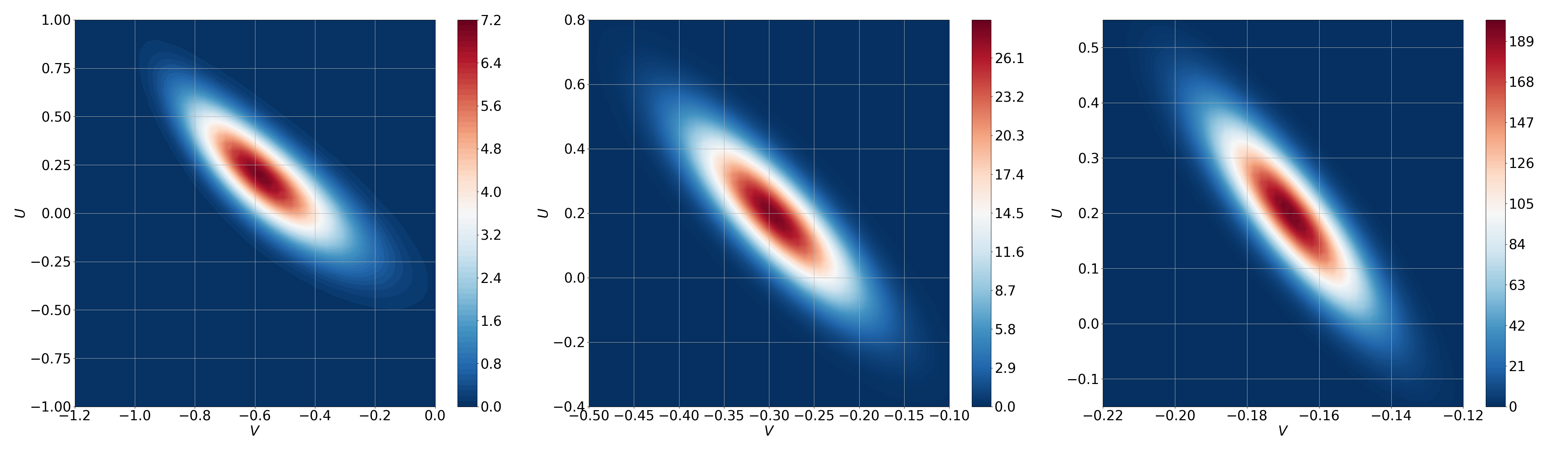
Figure 2: Contours of the benchmark densities $\displaystyle p_{\Delta}^{(\mathrm{B})}$. Left: $\displaystyle\Delta=0.1$. Middle: $\displaystyle\Delta=0.05$. Right: $\displaystyle\Delta=0.02$.

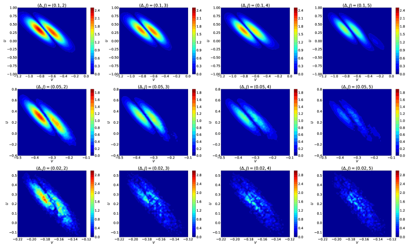
Figure 3: Absolute error by the density expansion II (DE-II).

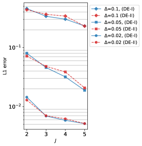
((a)) $\displaystyle L_{1}$-error

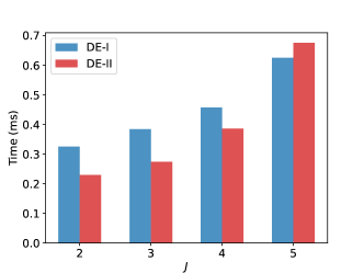
((b)) Computational time per grid

Figure 4: Summary for performance of density expansions.

4.2 Application to Bayesian Inference

4.2.1 MCMC via CF-expansion – Design of Posterior

We use our CF-expansion to carry out Bayesian inference for SDEs. In this subsection we consider general SDEs rather than just the FHN SDE as the approach is relevant in a wide setting. Via the CF-expansion we obtain a posterior law that can be integrated within well-established MCMC methodologies, including centred/non-centred parameterisations (Papaspiliopoulos et al., 2007), Particle MCMC and Particle Gibbs algorithms (Andrieu et al., 2010). Note that early literature (Stramer et al., 2010) investigated the use of CF-expansions (for elliptic models) within a standard Metropolis-Hastings method under centred parametrisation, thus the options provided were limited. Particle-based MCMC methods require sampling from the SDE transition density, i.e. in our case from the CF-expansion used as its proxy. It is typically difficult to simulate from the CF-expansion. However, notice that the expansion writes as ‘Gaussian density’ $\displaystyle\times$ ‘correction term’. Thus, particle-based MCMC and general Sequential Monte Carlo (SMC) methodology can be implemented using the baseline density (which we can sample from) with the correction term being attached in the ‘weights’ within the algorithm. Furthermore, the CF-expansion structure of ‘Gaussian density’ $\displaystyle\times$ ‘correction term’ permits a non-centred approach – such an algorithm turns out to be the most effective one in our numerics in the next section. We provide more details on the mentioned algorithms directly below.

Consider the data $\displaystyle\mathscr{Y}_{n}=\{Y_{t_{k}}\}_{0\leq k\leq n}$ at instances $\displaystyle t_{k}$, $\displaystyle 0\leq k\leq n$, for which we assume an equidistant step-size $\displaystyle\Delta$. We consider the setting of noisy observations, so that there is a density $\displaystyle p(Y_{t_{k}}|X_{t_{k}})$, assumed known. Under a data augmentation approach, we set $\displaystyle\mathbf{q}:=(\theta,\mathscr{X}_{n})\in\mathbb{R}^{d_{\theta}}\times\mathbb{R}^{N\times(n+1)}$, where $\displaystyle\mathscr{X}_{n}:=\{X_{t_{k}}\}_{1\leq k\leq n}$. The posterior density on the augmented state $\displaystyle\mathbf{q}=(\theta,\mathscr{X}_{n})$ writes as:

$$\displaystyle{P}(\mathbf{q}\,|\,\mathscr{Y}_{n})\propto\Bigl{\{}\prod_{k=0}^{n}p(Y_{t_{k}}|X_{t_{k}})\Bigr{\}}\times\Bigl{\{}\prod_{k=1}^{n}p_{\Delta}^{X}(X_{t_{k-1}},X_{t_{k}};\theta)\Bigr{\}}\times p_{0}(X_{0})\times p_{\theta}(\theta),$$ (4.4)

where $\displaystyle p_{0}$, $\displaystyle p_{\theta}$ denote priors on the initial value $\displaystyle X_{0}$ and the parameter $\displaystyle\theta$, respectively. We replace the true transition density with the CF-expansion as given in (3.12), that is:

$$\displaystyle\prod_{k=1}^{n}p_{\Delta}^{X}(X_{t_{k-1}},X_{t_{k}};\theta)\approx\prod_{k=1}^{n}p_{\Delta}^{\bar{X}}(X_{t_{k-1}},X_{t_{k}};\theta)\times\prod_{k=1}^{n}\exp\Bigl{(}T_{J^{\prime}}\bigl{(}\pi^{[J]}(\Delta,X_{t_{k-1}},X_{t_{k}};\theta)\bigr{)}\Bigr{)}.$$ (4.5)

The approximate posterior obtained via (4.4)-(4.5) can now be used within standard or particle-based MCMC methods: (i) For standard MCMC, the ‘correction terms’ can be treated as a part of the likelihood function, so that a-priori the dynamics of the $\displaystyle X$-process are determined by the baseline density. This allows for application of centred/non-centred algorithms, as in the latter case one can use as latent components the standard Gaussian noise that generates samples from the baseline density; (ii) For particle-based methods, the ‘correction terms’ can become part of the weights and one can apply, e.g., particle filters by sampling from the tractable baseline density.

4.2.2 Experimental Design and MCMC Results

We apply our CF-expansion to carry out Bayesian inference for the FHN SDE (4.1) with the real dataset used in Samson et al. (2024). The data are available at https://data.mendeley.com/datasets/ybhwtngzmm/1 which provides 20 neural recordings of the 5th lumbar dorsal rootlet from a single adult female rat with time length $\displaystyle 250$ms and equidistant step-size $\displaystyle 0.02$ms. In our study we choose a particular dataset, specifically the file 1554.mat from the above URL, which was obtained while the 5th lumber dermatome was stimulated. We subsample the first $\displaystyle 40$ms of data with a step-size $\displaystyle 0.08$ms, i.e. we have $\displaystyle(T,\Delta)=(40,0.08)$ and a number of datapoints $\displaystyle n=501$, so $\displaystyle\Delta$ is relatively large. As in Samson et al. (2024), we set $\displaystyle s=0$ and focus on the parameter $\displaystyle\theta=(\epsilon,\gamma,\beta,\sigma)$. We assume that the data $\displaystyle\mathscr{Y}_{n}=\{Y_{t_{k}}\}_{0\leq k\leq n}$ are observed with a small measurement noise as $\displaystyle Y_{t_{k}}=V_{t_{k}}+\epsilon_{t_{k}}$, with $\displaystyle V$ the smooth coordinate in the FHN SDE and $\displaystyle\epsilon_{t_{0}},\ldots,\epsilon_{t_{n}}\overset{i.i.d}{\sim}\mathscr{N}(0,0.01^{2})$. We adopt a non-centred parametrisation, assign log-normal priors on $\displaystyle\theta$, i.e., $\displaystyle\log\varepsilon,\log\beta,\log\gamma,\log\sigma\overset{\mathrm{i.i.d.}}{\sim}\mathscr{N}(0,1)$ and set $\displaystyle V_{0}\sim\mathscr{N}(0,0.1^{2}),\,U_{0}\sim\mathscr{N}(0,0.2^{2})$ for the initial state. We employ Hybrid Monte Carlo (HMC) to sample from the posterior, using the Python package Mici (https://pypi.org/project/mici/) which offers a variety of MCMC methods based on Hamiltonian dynamics. We use a dynamic integration-time HMC implementation (Betancourt, 2017) with a dual-averaging algorithm (Hoffman et al., 2014) to adapt the step-size of the leapfrog integrator. The mass matrix is set to identity.

We consider 3 designs of tractable posteriors: [P0] Benchmark ‘true’ posterior. This is constructed via a local Gaussian (LG) transition density scheme (Gloter and Yoshida, 2021), which provides an approximation of the transition density of the hypo-elliptic SDE (H) for a sufficiently small step-size. A data augmentation step is applied, whereby $\displaystyle d_{M}=100$ signal points are added in-between observation pairs to eliminate the bias. The obtained posterior values are treated as the benchmark true values; [P1] Posterior based on the partial LDL scheme given in (4.3) with $\displaystyle\iota=\mathrm{II}$; [P2] Posterior produced via implementation of the non-centred parameterisation of the initial target given by (4.4)-(4.5), based on the CF-expansion around the partial LDL scheme with $\displaystyle J=3$. For each posterior, we run two HMC chains of 8,000 iterations with the first 4,000 iterations used as an adaptive warm-up phase.

Fig. 5 shows results for targets P0-P2. Results for the true posterior P0 are given in black and are overlaid in the sub-figures to observe the accuracy of posteriors P1-P2. Table 1 shows average running times per iteration from two chains. Additional convergence diagnostics provided in Table 2 of Appendix 9.2 show similarly good convergence performance for all $\displaystyle 3$ cases, we can thus conclude that the posteriors shown in Fig. 5 are reliable. In Fig. 5 it is clear that P2 (i.e. scheme based upon the CF-expansion) captures P0 more accurately than P1 (i.e. scheme without correction terms) does. Thus, the inclusion of the correction term eliminates the bias even for $\displaystyle J=3$, with the algorithm targeting P2 having a computing cost approximately 10 times smaller than that of the benchmark P0 (see Table 1). Our experiment implies that, in this case, the CF-expansion is effective both from the perspectives of computational cost and estimation accuracy. We remark that a centred-parametrisation led to MCMC chains with very poor convergence performance.

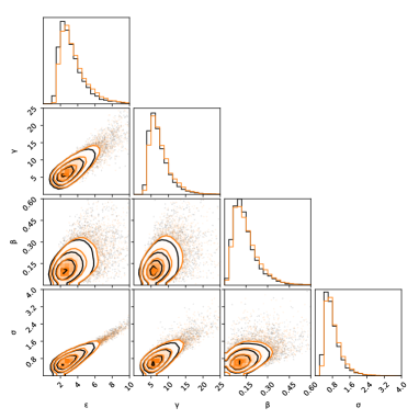
((a)) P1 (Partial LDL scheme)

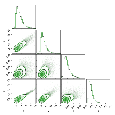
((b)) P2 (CF-expansion with $\displaystyle J=3$)

Figure 5: Posterior estimates. P0 (benchmark posterior) is overlaid in each figure in black.

Table 1: Computational cost of MCMC chains for the FHN model. Schemes: P0$\displaystyle\rightarrow$ benchmark; P2$\displaystyle\rightarrow$ Modified LDL; P3$\displaystyle\rightarrow$ CF-Expansion, $\displaystyle J=3$.

scheme	P0	P1	P2
time(sec)/iter	4.745	0.237	0.460

5 Conclusion

We propose a new CF-expansion for the transition density of multivariate SDEs over a time interval with fixed length $\displaystyle\Delta\in(0,1)$, of the form ‘baseline Gaussian density’ $\displaystyle\times$ ‘correction term’, where the ‘correction term’ involves quantities of size $\displaystyle\Delta^{j/2}$, $\displaystyle j=0,\ldots,J$, for $\displaystyle J\geq 1$. Analytical expressions can be obtained via any software that carries out symbolic calculations. We have shown analytically that the error has a size of $\displaystyle\mathcal{O}(\Delta^{(J+1)/2})$. The proposed CF-expansion covers hypo-elliptic classes of SDEs, whereas CF-expansions in earlier works are designed only for elliptic SDEs. In the numerical studies in Section 4 the errors from our CF-expansion are fastly eliminated as $\displaystyle J$ increases for a fixed $\displaystyle\Delta\in(0,1)$.

We also mention the following. First, we take the direction described in the paper to produce our CF-expansion because potential alternative approaches used in the literature for the elliptic class (involving, e.g., Malliavin calculus) are arguably much more challenging in terms of producing a practical and theoretically validated methodolology. Second, several recent works on the theme of parameter inference for hypo-elliptic SDEs produce methodology and analytical results in the high-frequency scenario $\displaystyle\Delta\rightarrow 0$, see e.g. Ditlevsen and Samson (2019); Melnykova (2020); Gloter and Yoshida (2021); Pilipovic et al. (2024); Iguchi and Beskos (2023); Iguchi et al. (2024, 2025). Then, numerical experiments are used to check the precision for a fixed $\displaystyle\Delta>0$ given in practice. In contrast, our contribution assumes a fixed $\displaystyle\Delta$, thus is expected to be more robust in deviations of $\displaystyle\Delta$ from $\displaystyle 0$ than high-frequency approaches. Finally, we stress that our CF-expansion converges exponentially fast with $\displaystyle J\geq 1$, so small values of $\displaystyle J$ will typically provide accurate proxies. Such a consideration counterbalances the scaling of the computing cost for increasing state dimension $\displaystyle N$. Following the analytical expressions of the $\displaystyle e_{k}$’e for the FHN model in Appendix 9 of the Supplementary Material, in the case of additive noise one has $\displaystyle e_{1}=e_{2}=0$, while the calculation of $\displaystyle e_{5}$ requires all 3rd order derivatives of the baseline Gaussian density, at a cost of $\displaystyle\mathcal{O}(N^{3})$. An extra derivative is added in the calculation when increasing $\displaystyle k$ in $\displaystyle e_{k}$ by one. Note that calculations involving just the baseline Gaussian transition density will typically already involve costs of $\displaystyle\mathcal{O}(N^{3})$ due to matrix inversions, so in the additive noise setting using $\displaystyle J=5$ will not increase computing costs vs $\displaystyle J=0$ as an order of $\displaystyle N$.

Supplmentary Material

The material is organised as follows: Section 6 provides proof of Lemmas 2.1, 2.2, 2.3. In Section 7, we prove Lemma 3.1 and the central analytic results provided in the main text, i.e., Theorems 1 and 2, error estimates for the proposed CF expansion. Section 8 studies the expression of the differential operator $\displaystyle\mathscr{D}_{\alpha}^{z,\theta}$ given in (2.21). Section 9 provides supporting information for the implementation of density expansion used in the numerical experiments and additional experiments of Bayesian inference for FHN model.

6 Proof of Lemmas 2.1, 2.2, and 2.3

6.1 Proof of Lemma 2.1

We write the LDL scheme (2.11) with a frozen variable $\displaystyle z\in\mathbb{R}^{N}$ as the following differential form:

$$\displaystyle d\bar{X}_{t}^{\theta,z}={V}_{0}^{z}(\bar{X}_{t}^{\theta,z},\theta)dt+\sum_{j=1}^{d}V_{j}^{z}(\bar{X}_{t}^{\theta,z},\theta)dB_{j,t},\quad X_{0}=x,$$

for $\displaystyle(x,\theta)\in\mathbb{R}^{N}\times\Theta$, where we have set:

$$\displaystyle V_{0}^{z}(x,\theta)\equiv A_{z,\theta}x+b_{z,\theta},\qquad V_{j}^{z}(x,\theta)\equiv V_{j}(z,\theta),\quad 1\leq j\leq d.$$ (6.1)

Since the diffusion coefficients are independent of the state $\displaystyle\bar{X}_{t}^{\theta,z}$, the above Itô-type SDE identifies with the Stratonovich one. We show under Assumption 2 that the vector fields determined from the coefficients of the above SDE satisfy Hörmander’s condition for each model class E and H.

Elliptic model E. We immediately have from Assumption 2-I that

$$\displaystyle\mathrm{Span}\bigl{\{}V_{j}^{z}(x,\theta)|_{z=x},\ \ 1\leq j\leq d\bigr{\}}=\mathbb{R}^{N},$$ (6.2)

for all $\displaystyle(x,\theta)\in\mathbb{R}^{N}\times\Theta$.

Hypo-elliptic model H. We firstly note that

$$\displaystyle\widetilde{V}_{S,0}(x,\theta)\equiv{V}_{S,0}(x,\theta),\quad V_{j}^{z}(x,\theta)\equiv\bigl{[}\mathbf{0}_{N_{S}}^{\top},V_{R,j}(z,\theta)^{\top}\bigr{]}^{\top},\qquad 1\leq j\leq d.$$

Then Assumption 2-II is equivalent to the following condition:

$$\displaystyle\begin{aligned} \mathrm{Span}\bigl{\{}V_{R,j}(x,\theta),\,1\leq j\leq d\bigr{\}}&=\mathbb{R}^{N_{R}};\\ \mathrm{Span}\bigl{\{}\mathrm{Proj}_{1,N_{S}}\{[\widetilde{V}_{0},V_{j}](x,\theta)\},\,1\leq j\leq d\bigr{\}}&=\mathrm{Span}\bigl{\{}\partial_{x_{R}}^{\top}V_{S,0}(x,\theta)V_{R,j}(x,\theta),\,1\leq j\leq d\bigr{\}}=\mathbb{R}^{N_{S}}.\end{aligned}$$ (6.3)

The condition (6.3) leads to:

$$\displaystyle\mathrm{Span}\bigl{\{}V_{R,j}(z,\theta)|_{z=x},\,1\leq j\leq d\bigr{\}}=\mathbb{R}^{N_{R}},$$

and

$$\displaystyle\mathrm{Span}\bigl{\{}\mathrm{Proj}_{1,N_{S}}\bigl{\{}[V_{0}^{z},V_{j}^{z}](x,\theta)|_{z=x}\bigr{\}},\,1\leq j\leq d\bigr{\}}=\mathrm{Span}\bigl{\{}\mathrm{Proj}_{1,N_{S}}\{A_{z,\theta}V_{j}^{z}(x,\theta)|_{z=x}\},\,1\leq j\leq d\bigr{\}}$$

$$\displaystyle\qquad=\mathrm{Span}\bigl{\{}\partial_{x_{R}}^{\top}V_{S,0}(z,\theta)V_{R,j}(z,\theta)|_{z=x},\,1\leq j\leq d\bigr{\}}=\mathbb{R}^{N_{S}}.$$

Thus, we obtain:

$$\displaystyle\mathrm{Span}\Bigl{\{}\bigl{\{}V_{j}^{z}(x,\theta),[V_{0}^{z},V_{j}^{z}](x,\theta)\bigr{\}}|_{z=x},\,1\leq j\leq d\Bigr{\}}=\mathbb{R}^{N},$$ (6.4)

for all $\displaystyle(x,\theta)\in\mathbb{R}^{N}\times\Theta$. The proof of Lemma 2.1 is now complete.

6.2 Proof of Lemma 2.2

We define

$$\displaystyle G(s)\equiv\int_{\mathbb{R}^{N}}p^{\bar{X}^{z}}_{\Delta-s}(\xi,y;\theta)p^{X}_{s}(x,\xi;\theta)|_{z=x}\,d\xi,\qquad s\geq 0.$$ (6.5)

Noticing that $\displaystyle p^{X}_{0}(x,y;\theta)=\delta_{y}(x)$ and $\displaystyle p^{\bar{X}}_{0}(x,y;\theta)=\delta_{y}(x)$, we have

$$\displaystyle p^{X}_{\Delta}(x,y;\theta)-p^{\bar{X}^{z}}_{\Delta}(x,y;\theta)|_{z=x}=G(\Delta)-G(0)=\int_{0}^{\Delta}G^{\prime}(s)ds.$$

Also, note that the transition densities $\displaystyle p^{X}_{\Delta}(x,y;\theta)$ and $\displaystyle p^{\bar{X}^{z}}_{\Delta}(x,y;\theta)$ satisfy the following backward/forward Kolmogorov equations:

$$\displaystyle\partial_{t}\,p^{X}_{t}(x,y;\theta)=\mathscr{L}_{\theta}\{p^{X}_{t}(\cdot,y;\theta)\}(x),\qquad\partial_{t}\,p^{X}_{t}(x,y;\theta)=\mathscr{L}_{\theta}^{*}\{p^{X}_{t}(x,\cdot;\theta)\}(y);$$ (6.6)

$$\displaystyle\partial_{t}\,p^{\bar{X}^{z}}_{t}(x,y;\theta)=\mathscr{L}_{\theta}^{0,z}\{p^{\bar{X}^{z}}_{t}(\cdot,y;\theta)\}(x).$$ (6.7)

Then it follows that

$$\displaystyle G^{\prime}(s) \displaystyle=-\int_{\mathbb{R}^{N}}\mathscr{L}_{\theta}^{0,z}\{p^{\bar{X}^{z}}_{\Delta-s}(\cdot,y;\theta)\}(\xi)p^{X}_{s}(x,\xi;\theta)|_{z=x}d\xi+\int_{\mathbb{R}^{N}}p^{\bar{X}^{z}}_{\Delta-s}(\xi,y;\theta)\mathscr{L}_{\theta}^{\ast}\{p^{X}_{s}(x,\cdot;\theta)\}(\xi)|_{z=x}d\xi$$

$$\displaystyle=-\int_{\mathbb{R}^{N}}\mathscr{L}_{\theta}^{0,z}\{p^{\bar{X}^{z}}_{\Delta-s}(\cdot,y;\theta)\}(\xi)p^{X}_{s}(x,\xi;\theta)|_{z=x}d\xi+\int_{\mathbb{R}^{N}}\mathscr{L}_{\theta}\{p^{\bar{X}^{z}}_{\Delta-s}(\cdot,y;\theta)\}(\xi)p^{X}_{s}(x,\xi;\theta)|_{z=x}d\xi.$$

The proof of Lemma 2.2 is now complete.

6.3 Proof of Lemma 2.3

We focus on showing the formula (2.16), and (2.17) is obtained from a similar argument. We make use of the approach used in Iguchi and Yamada (2021, Proposition 2.1). We define

$$\displaystyle g^{\widetilde{\mathscr{L}}^{z}_{\theta}}(s) \displaystyle\equiv\bar{P}_{s}^{\theta,z}\widetilde{\mathscr{L}}^{z}_{\theta}\bar{P}_{t-s}^{\theta,z}\varphi(x)=\int_{\mathbb{R}^{N}}\widetilde{\mathscr{L}}^{z}_{\theta}\bar{P}_{t-s}^{\theta,z}\varphi(\xi)\,p^{\bar{X}^{z}}_{s}(x,\xi_{1};\theta)\,d\xi_{1}$$ (6.8)

and consider the Taylor expansion of $\displaystyle g^{\widetilde{\mathscr{L}}^{z}_{\theta}}(s)$ at $\displaystyle s=0$:

$$\displaystyle g^{\widetilde{\mathscr{L}}^{z}_{\theta}}(s) \displaystyle=\sum_{k=0}^{J}\partial^{k}g^{\widetilde{\mathscr{L}}^{z}_{\theta}}(s)|_{s=0}\times\frac{s^{k}}{k!}+\mathscr{R}^{J+1,z}(s,t,x;\theta),\qquad J\in\mathbb{N},$$ (6.9)

where $\displaystyle\textstyle\mathscr{R}^{J+1,z}(s,t,x;\theta)\equiv{s^{J+1}}\int_{0}^{1}\partial^{J+1}g^{\widetilde{\mathscr{L}}^{z}_{\theta}}(su)\tfrac{(1-u)^{J}}{J!}du$. We have from (6.8) that

$$\displaystyle\partial g^{\widetilde{\mathscr{L}}^{z}_{\theta}}(s)=\int_{\mathbb{R}^{N}}\widetilde{\mathscr{L}}^{z}_{\theta}\bar{P}_{t-s}^{\theta,z}\varphi(\xi_{1})\,\partial_{s}p^{\bar{X}^{z}}_{s}(x,\xi_{1};\theta)\,d\xi_{1}+\int_{\mathbb{R}^{N}}\widetilde{\mathscr{L}}^{z}_{\theta}\partial_{s}\bar{P}_{t-s}^{\theta,z}\varphi(\xi_{1})\,p^{\bar{X}^{z}}_{s}(x,\xi_{1};\theta)\,d\xi_{1}$$

$$\displaystyle=\int_{\mathbb{R}^{N}}\widetilde{\mathscr{L}}^{z}_{\theta}\bar{P}_{t-s}^{\theta,z}\varphi(\xi_{1})\,(\mathscr{L}_{\theta}^{0,z})^{\ast}\{p^{\bar{X}^{z}}_{s}(x,\cdot;\theta)\}(\xi_{1})\,d\xi_{1}-\int_{\mathbb{R}^{N}}\widetilde{\mathscr{L}}^{z}_{\theta}\mathscr{L}_{\theta}^{0,z}\bar{P}_{t-s}^{\theta,z}\varphi(\xi_{1})\,p^{\bar{X}^{z}}_{s}(x,\xi_{1};\theta)\,d\xi_{1}$$

$$\displaystyle=\int_{\mathbb{R}^{N}}[\mathscr{L}_{\theta}^{0,z},\widetilde{\mathscr{L}}^{z}_{\theta}]\bar{P}_{t-s}^{\theta,z}\varphi(\xi_{1})\,p^{\bar{X}^{z}}_{s}(x,\xi_{1};\theta)\,d\xi_{1}$$

$$\displaystyle=g^{[\mathscr{L}_{\theta}^{0,z},\widetilde{\mathscr{L}}^{z}_{\theta}]}(s),$$

where we made use of (6.7) and integration by parts in the second and third lines, respectively. Thus, the higher-order derivatives of $\displaystyle g^{\widetilde{\mathscr{L}}^{z}_{\theta}}(s)$ are given as:

$$\displaystyle\partial^{k}g^{\widetilde{\mathscr{L}}^{z}_{\theta}}(s)=g^{(\mathrm{ad}_{\mathscr{L}_{\theta}^{0,z}})^{k}(\widetilde{\mathscr{L}}_{\theta}^{z})}(s)=\bar{P}_{s}^{\theta,z}\bigl{\{}\bigl{(}\mathrm{ad}_{\mathscr{L}_{\theta}^{0,z}}\bigr{)}^{k}(\widetilde{\mathscr{L}}_{\theta}^{z})\bigr{\}}\bar{P}_{t-s}^{\theta,z}\varphi(x),\qquad 0\leq k\leq J,$$ (6.10)

and then,

$$\displaystyle\partial^{k}g^{\widetilde{\mathscr{L}}^{z}_{\theta}}(s)|_{s=0}=\bigl{\{}\bigl{(}\mathrm{ad}_{\mathscr{L}_{\theta}^{0,z}}\bigr{)}^{k}(\widetilde{\mathscr{L}}_{\theta}^{z})\bigr{\}}\bar{P}_{t}^{\theta,z}\varphi(x).$$ (6.11)

The proof of Lemma 2.3 is now complete.

7 Proof of Lemma 3.1 and Theorems 1-2

This section is organised as follows: In Section 7.1, we collect notations and basic results that are frequently used throughout Section 7. In Section 7.2, we show Lemma 3.1. Section 7.3 provides five auxiliary results (Propositions 7.1, 7.2, 7.3 and Lemmas 7.1, 7.2) to prove the main analytic results (Theorems 1 and 2). Propositions 7.2 and 7.3 in particular play a central role to show Theorems 1 and 2, respectively. Proposition 7.1 and Lemmas 7.1–7.2 are required to show Propositions 7.2–7.3. Given Propositions 7.2 and 7.3, we prove Theorems 1 and 2 in Section 7.4 and 7.5, respectively.

7.1 Preliminaries

We introduce and recall notations frequently used throughout Section 7.

• For $\displaystyle x,y,z\in\mathbb{R}^{N},\,\theta\in\Theta$, $\displaystyle 0\leq s\leq t<\infty$ and $\displaystyle w\in\{\ref{eq:ellip},\ref{eq:hypo}\}$,

  $$\displaystyle\Gamma_{t,(\ref{eq:ellip})}\equiv\mathrm{diag}\bigl{(}\underbrace{\sqrt{t},\ldots,\sqrt{t}}_{N}\bigr{)},\quad\Gamma_{t,(\ref{eq:hypo})}\equiv\mathrm{diag}\bigl{(}\underbrace{\sqrt{t^{3}},\ldots,\sqrt{t^{3}}}_{N_{S}},\underbrace{\sqrt{t},\ldots,\sqrt{t}}_{N_{R}}\bigr{)};$$ (7.1)

  $$\displaystyle\nu^{(w),z}(t,y,x,\theta)\equiv\Gamma_{t,(w)}^{-1}\Bigl{(}e^{-tA_{z,\theta}}y-x-\int_{0}^{t}e^{-sA_{z,\theta}}b_{z,\theta}ds\Bigr{)};$$ (7.2)

  $$\displaystyle v(t,s,y,x,\theta)\equiv x+V_{0}(x,\theta)s-e^{-(t-s)A_{x,\theta}}y+\int_{0}^{t-s}e^{-uA_{x,\theta}}b_{x,\theta}du.$$ (7.3)

• Recall:

  $$m(\ref{eq:ellip})\equiv N,\quad m(\ref{eq:hypo})\equiv 4d$$

  and for $\displaystyle\alpha\in\mathbb{Z}_{\geq 0}^{N}$,

  $$\displaystyle\|\alpha\|_{\ref{eq:ellip}}\equiv\tfrac{1}{2}|\alpha|,\qquad\|\alpha\|_{\ref{eq:hypo}}\equiv\tfrac{3}{2}|\alpha_{S}|+\tfrac{1}{2}|\alpha_{R}|$$ (7.4)

  with convention $\displaystyle\alpha_{S}=(\alpha_{1},\ldots,\alpha_{N_{S}})$ and $\displaystyle\alpha_{R}=(\alpha_{N_{S}+1},\ldots,\alpha_{N})$ for hypo-elliptic model $\displaystyle\eqref{eq:hypo}$.

• Let $\displaystyle\mathscr{F}^{(w)},\,w\in\{\ref{eq:ellip},\ref{eq:hypo}\}$ be a space of functions $\displaystyle\psi^{(w)}:(0,1)\times\mathbb{R}^{N}\to\mathbb{R},\,w\in\{\ref{eq:ellip},\ref{eq:hypo}\}$ satisfying the following property: for any $\displaystyle\alpha\in\mathbb{Z}_{\geq 0}^{N}$, there exists a constant $\displaystyle C>0$ such that for all $\displaystyle(t,\xi)\in(0,1)\times\mathbb{R}^{N}$,

  $$\displaystyle\bigl{|}\partial_{\xi}^{\alpha}\psi^{(w)}(t,\xi)\bigr{|}\leq Ct^{-\|\alpha\|_{w}}\times\bigl{|}\widetilde{\psi}^{(w)}(t,\xi)\bigr{|},$$ (7.5)

  for some function $\displaystyle\widetilde{\psi}^{(w)}:(0,1)\times\mathbb{R}^{N}\to\mathbb{R}$.

• For $\displaystyle\kappa>0$ defined in Assumption 4,

  $$\displaystyle\mathscr{Z}_{\kappa}\equiv\bigl{\{}\xi\in\mathbb{R}^{N}\,\bigl{|}\,|\xi|+\bigl{|}V_{0}(\xi,\theta)\bigr{|}\leq\kappa,\quad\forall\ \theta\in\Theta\bigr{\}}.$$ (7.6)

  In particular, under Assumption 4, the initial state $\displaystyle x$ is an element of $\displaystyle\mathscr{Z}_{\kappa}$.

• Let $\displaystyle\mathscr{G}^{(w)}:(0,\infty)\times\mathbb{R}^{N}\times\mathbb{R}^{N}\times\Theta\to\mathbb{R}$ and $\displaystyle\overline{\mathscr{G}}^{(w),z}:(0,\infty)\times\mathbb{R}^{N}\times\mathbb{R}^{N}\times\Theta\to\mathbb{R},\,w\in\{\ref{eq:ellip},\ref{eq:hypo}\}$, $\displaystyle z\in\mathscr{Z}_{\kappa}$ be generic notations to represent functions having the following property: there exist constants $\displaystyle C,\lambda>0$ such that for all $\displaystyle(t,x,y,z,\theta)\in(0,\infty)\times\mathbb{R}^{N}\times\mathbb{R}^{N}\times\mathscr{Z}_{\kappa}\times\Theta$,

  $$\displaystyle\bigl{|}{\mathscr{G}}^{(w)}(t,x,y,\theta)\bigr{|} \displaystyle\leq Ct^{-\tfrac{m(w)}{2}}\exp\Bigl{(}-\lambda\bigl{|}\Gamma_{t,(w)}^{-1}\bigl{(}y-x-V_{0}(x,\theta)t\bigr{)}\bigr{|}^{2}\Bigr{)};$$

  $$\displaystyle\bigl{|}\overline{\mathscr{G}}^{(w),z}(t,x,y,\theta)\bigr{|} \displaystyle\leq Ct^{-\tfrac{m(w)}{2}}\exp\Bigl{(}-\lambda\bigl{|}\nu^{(w),z}(t,y,x,\theta)\bigr{|}^{2}\Bigr{)},$$ (7.7)

  where $\displaystyle\Gamma_{t,(w)}$ and $\displaystyle\nu^{(w),z}$ are defined in (7.1) and (7.2), respectively.

• For a differential operator $\displaystyle D$ acting on the functions over $\displaystyle\mathbb{R}^{N}$, we write $\displaystyle D^{\ast}$ as its adjoint defined via the formula: $\displaystyle\textstyle\int_{\mathbb{R}^{N}}Df(x)g(x)dx=\int_{\mathbb{R}^{N}}f(x)D^{\ast}g(x)dx$, for sufficiently smooth functions $\displaystyle f,g\in L^{2}(\mathbb{R}^{N})$ vanishing at infinity.

The following basic results/estimates are frequently used throughout Section 7:

1. For $\displaystyle\alpha\in\mathbb{Z}_{\geq 0}^{N}$, it holds that

   $$\displaystyle\partial^{\alpha}_{y}p_{t}^{\bar{X}^{z}}(x,y;\theta)=\partial^{\alpha}_{x}p_{t}^{\bar{X}^{z}}(x,y;\theta)G_{\alpha}^{z}(t,\theta),\qquad(t,x,y,z,\theta)\in(0,\infty)\times\mathbb{R}^{N}\times\mathbb{R}^{N}\times\mathscr{Z}_{\kappa}\times\Theta,$$ (7.8)

   where $\displaystyle G_{\alpha}^{z}:(0,\infty)\times\Theta\to\mathbb{R}$ satisfies the following property under Assumptions 3–4:

   $$\displaystyle\sup_{(t,z,\theta)\in(0,1)\times\mathscr{Z}_{\kappa}\times\Theta}\bigl{|}G_{\alpha}^{z}(t,\theta)\bigr{|}<\infty.$$

2. For two multidimensional Gaussian densities $\displaystyle\mathbb{R}^{N}\ni\xi\mapsto\varphi(\xi;a_{i},A_{i}),\,i=1,2$ with mean $\displaystyle a_{i}\in\mathbb{R}^{N}$ and covariance $\displaystyle A_{i}\in\mathbb{R}^{N\times N}$, it follows (see e.g. Vinga (2004)) that:

   $$\displaystyle\begin{aligned} \int_{\mathbb{R}^{N}}\varphi_{1}(\xi;a_{1},A_{1})\varphi_{2}(\xi;a_{2},A_{2})d\xi=\tfrac{1}{\sqrt{(2\pi)^{N}\det\bigl{(}A_{1}+A_{2}\bigr{)}}}\exp\Bigl{(}-\tfrac{1}{2}(a_{1}-a_{2})^{\top}(A_{1}+A_{2})^{-1}(a_{1}-a_{2})\Bigr{)}.\end{aligned}$$ (7.9)

3. Let $\displaystyle\lambda_{1}>0$. For any $\displaystyle\alpha\in\mathbb{Z}_{\geq 0}^{N}$, there exist constants $\displaystyle c,\lambda_{2}>0$ such that for all $\displaystyle\xi\in\mathbb{R}^{N}$,

   $$\displaystyle|\xi^{\alpha}|\times\exp\bigl{(}-\lambda_{1}|\xi|^{2}\bigr{)}\leq C\exp\bigl{(}-\lambda_{2}|\xi|^{2}\bigr{)}.$$ (7.10)

   We note that this type of inequality is also used to prove the bound of the remainder term of density expansion for elliptic diffusions in Yang et al. (2019).

7.2 Proof of Lemma 3.1

We will show the following statement: it holds under Assumptions 1–5 that for the initial state $\displaystyle x\in\mathbb{R}^{N}$, $\displaystyle(\Delta,y,z,\theta)\in(0,\infty)\times\mathbb{R}^{N}\times\mathscr{Z}_{\kappa}\times\Theta$,

$$\displaystyle\partial^{\alpha}_{x}\,p_{\Delta}^{\bar{X}^{z},(w)}(x,y;\theta) \displaystyle=\Delta^{-\|\alpha\|_{w}}\times\mathscr{H}^{(w),z}_{\alpha}(\Delta,x,y,\theta)\,p_{\Delta}^{\bar{X}^{z},(w)}(x,y;\theta),\quad\alpha\in\mathbb{Z}_{\geq 0}^{N},\quad w\in\{\ref{eq:ellip},\ref{eq:hypo}\},$$ (7.11)

for some $\displaystyle\mathscr{H}_{\alpha}^{(w),z}:(0,\infty)\times\mathbb{R}^{N}\times\mathbb{R}^{N}\times\Theta\to\mathbb{R}$ satisfying that there exists a constant $\displaystyle C>0$ such that for all $\displaystyle(\Delta,x,y,z,\theta)\in(0,1)\times\mathbb{R}^{N}\times\mathbb{R}^{N}\times\mathscr{Z}_{\kappa}\times\Theta$,

$$\displaystyle\bigl{|}\mathscr{H}^{(w),z}_{\alpha}(\Delta,x,y,\theta)\,p_{\Delta}^{\bar{X}^{z},(w)}(x,y;\theta)\bigr{|}\leq C\Delta^{-\tfrac{m(w)}{2}}\exp\Bigl{(}-\lambda|\nu^{(m),z}(\Delta,y,x,\theta)|^{2}\Bigr{)}.$$

Note that the statement of Lemma 3.1 is immediately obtained by setting $\displaystyle z=x$ in (7.11).

We first consider the case $\displaystyle|\alpha|=1$, i.e. $\displaystyle\partial_{x}^{\alpha}\equiv\partial_{x_{j}},\,1\leq j\leq N$. We have that

$$\displaystyle p_{\Delta}^{\bar{X}^{z},(w)}(x,y;\theta)=\tfrac{1}{\sqrt{(2\pi)^{N}\det{\Sigma}(\Delta,z,y)}}\exp\Bigl{(}-\tfrac{1}{2}\nu^{(w),z}(\Delta,y,x,\theta)^{\top}\bigl{(}\mathscr{M}^{(w)}(\Delta,z,\theta)\bigr{)}^{-1}\nu^{(w),z}(\Delta,y,x,\theta)\Bigr{)}$$ (7.12)

with $\displaystyle\mathscr{M}^{(w)}(\Delta,z,\theta)\equiv\Gamma_{\Delta,(w)}^{-1}\hat{\Sigma}(\Delta,z,\theta)\Gamma_{\Delta,(w)}^{-1}$, where the matrices $\displaystyle{\Sigma},\hat{\Sigma}$ are defined in (2.5) in the main text and $\displaystyle\nu^{(w),z}$ in (7.2). Then,

$$\displaystyle\partial_{x_{j}}p_{\Delta}^{\bar{X}^{z},(w)}(x,y;\theta)=\Delta^{-\|(j)\|_{w}}\times\mathscr{H}_{(j)}^{(w),z}(\Delta,x,y,\theta)\times p_{\Delta}^{\bar{X}^{z},(w)}(x,y;\theta)$$ (7.13)

with

$$\displaystyle\mathscr{H}_{(j)}^{(w),z}(\Delta,x,y,\theta)=\sum_{1\leq k\leq N}\bigl{[}\bigl{(}\mathscr{M}^{(w)}(\Delta,z,\theta)\bigr{)}^{-1}\bigr{]}_{jk}\bigl{[}\nu^{(w),z}(\Delta,y,x,\theta)\bigr{]}_{k}.$$ (7.14)

We will show under Assumptions 2 and 4 that there exists a constant $\displaystyle C>0$ such that for all $\displaystyle(t,z,\theta)\in(0,1)\times\mathscr{Z}_{\kappa}\times\Theta$,

$$\displaystyle\Bigl{|}\bigl{[}\bigl{(}\mathscr{M}^{(w)}(t,z,\theta)\bigr{)}^{-1}\bigr{]}_{i_{1}i_{2}}\Bigr{|}\leq C,\qquad 1\leq i_{1},i_{2}\leq N,\quad w\in\{\ref{eq:ellip},\ref{eq:hypo}\}.$$ (7.15)

To check (7.15), we study the bound for the elements of the matrix $\displaystyle\hat{\Sigma}$. Due to the expansion $\displaystyle e^{-sA_{z,\theta}}=I_{N}-sA_{z,\theta}+\mathscr{O}(s^{2})$, we have under Assumption 4 that

$$\displaystyle\hat{\Sigma}(t,z,\theta)\equiv\int_{0}^{t}e^{-sA_{z,\theta}}\sigma(z,\theta)\sigma(z,\theta)^{\top}e^{-sA_{z,\theta}^{\top}}ds$$

$$\displaystyle=ta(z,\theta)^{\top}-\tfrac{t^{2}}{2}\bigl{(}A_{z,\theta}a(z,\theta)+a(z,\theta)A_{z,\theta}^{\top}\bigr{)}+\tfrac{t^{3}}{3}A_{z,\theta}a(z,\theta)A_{z,\theta}^{\top}+\widetilde{\Sigma}(t,z,\theta),$$

where the remainder term $\displaystyle\widetilde{\Sigma}(t,z,\theta)$ satisfies: $\displaystyle\sup_{(z,\theta)\in\mathscr{Z}_{\kappa}\times\Theta}\bigl{|}\widetilde{\Sigma}(t,z,\theta)\bigr{|}\leq Ct^{4}$ for some constant $\displaystyle C>0$ independent of $\displaystyle t\in(0,1)$. Note that under model class (H), the matrix $\displaystyle a(z,\theta)$ is degenerate, and also the matrix

$$ta(z,\theta)^{\top}-\tfrac{t^{2}}{2}\bigl{(}A_{z,\theta}a(z,\theta)+a(z,\theta)A_{z,\theta}^{\top}\bigr{)}+\tfrac{t^{3}}{3}A_{z,\theta}a(z,\theta)A_{z,\theta}^{\top}$$

is positive definite under Assumption 2. Thus, there exists a constant $\displaystyle C>0$ such that for all $\displaystyle(t,z,\theta)\in(0,1)\times\mathscr{Z}_{\kappa}\times\Theta$,

• under model class (E),

  $$\displaystyle[\hat{\Sigma}(t,z,\theta)]_{i_{1}i_{2}}\leq Ct,\qquad 1\leq i_{1},i_{2}\leq N,$$ (7.16)

• under model class (H),

  $$\displaystyle[\hat{\Sigma}(t,z,\theta)]_{i_{1}i_{2}}\leq\begin{cases}Ct^{3},&1\leq i_{1},i_{2}\leq N_{S};\\ Ct,&N_{S}+1\leq i_{1},i_{2}\leq N;\\ Ct^{2},&(\mathrm{otherwise}).\end{cases}$$ (7.17)

Then, the inequality (7.15) is deduced from (7.16) and (7.17). We also have from the positive definiteness of $\displaystyle\hat{\Sigma}$, (7.16) and (7.17) that: there exists a constant $\displaystyle c>0$ such that for all $\displaystyle(t,z,\theta)\in(0,1)\times\mathscr{Z}_{\kappa}\times\Theta$,

$$\displaystyle\det\Sigma(t,z,\theta)\geq c\times\begin{cases}t^{N}&\mathrm{under\,model\,class\,\eqref{eq:ellip}};\\ t^{4d}&\mathrm{under\,model\,class\,\eqref{eq:hypo}}.\end{cases}$$ (7.18)

Thus, it follows from (7.14), (7.15) and (7.18) that:

$$\displaystyle\Bigl{|}\mathscr{H}_{(j)}^{(w),z}(\Delta,x,y,\theta)\times p_{\Delta}^{\bar{X}^{z},(w)}(x,y;\theta)\Bigr{|} \displaystyle\leq C_{1}\bigl{|}\nu^{(w),z}(\Delta,y,x,\theta)\bigr{|}\times\Delta^{-\tfrac{m(w)}{2}}\exp\Bigl{(}-\lambda_{1}\bigl{|}\nu^{(w),z}(\Delta,y,x,\theta)\bigr{|}^{2}\Bigr{)}$$

$$\displaystyle\leq C_{2}\Delta^{-\tfrac{m(w)}{2}}\exp\Bigl{(}-\lambda_{2}\bigl{|}\nu^{(w),z}(\Delta,y,x,\theta)\bigr{|}^{2}\Bigr{)}\quad\bigl{(}\because\eqref{eq:exp_bd}\bigr{)}$$

for some constants $\displaystyle C_{1},C_{2},\lambda_{1},\lambda_{2}>0$ that are independent of $\displaystyle\Delta,x,y,z$ and $\displaystyle\theta$. Hence, the formula (7.11) holds with $\displaystyle|\alpha|=1$. (7.11) with $\displaystyle|\alpha|\geq 1$ can be shown via iterative application of (7.13) with a similar argument presented above, and we conclude. ∎

7.3 Auxiliary reesults for Theorems 1 and 2

Proposition 7.1.

Let Assumptions 1–5 hold. For any $\displaystyle\alpha\in\mathbb{Z}_{\geq 0}^{N}$, there exist constants $\displaystyle C,\lambda>0$ such that for all $\displaystyle(\Delta,y,\theta)\in(0,1)\times\mathbb{R}^{N}\times\Theta$,

$$\displaystyle\bigl{|}\partial^{\alpha}_{y}p_{\Delta}^{X,(w)}(x,y;\theta)\bigr{|} \displaystyle\leq C\Delta^{-\|\alpha\|_{w}-\tfrac{m(w)}{2}}\times\exp\Bigl{(}-\lambda\bigl{|}\Gamma_{\Delta,(w)}^{-1}\bigl{(}y-x-V_{0}(x,\theta)\Delta\bigr{)}\bigr{|}^{2}\Bigr{)},\qquad w\in\{\ref{eq:ellip},\ref{eq:hypo}\},$$ (7.19)

where we recall $\displaystyle\|\cdot\|_{w}$ is given in (7.4). Also, for any $\displaystyle\alpha\in\mathbb{Z}_{\geq 0}^{N}$, there exists a constant $\displaystyle C,\lambda>0$ such that for all $\displaystyle(\Delta,x,y,z,\theta)\in(0,1)\times\mathbb{R}^{N}\times\mathbb{R}^{N}\times\mathscr{Z}_{\kappa}\times\Theta$,

$$\displaystyle\Bigl{|}\partial^{\alpha}_{y}p_{\Delta}^{\bar{X}^{z},(w)}(x,y;\theta)\Bigr{|} \displaystyle\leq C\Delta^{-\|\alpha\|_{w}-\tfrac{m(w)}{2}}\times\exp\Bigl{(}-\lambda\bigl{|}\nu^{(w),z}(\Delta,y,x,\theta)\bigr{|}^{2}\Bigr{)},\qquad w\in\{\ref{eq:ellip},\ref{eq:hypo}\}.$$ (7.20)

Proof of Proposition 7.1. We first show (7.19). We have from (Pigato, 2022, Theorem 2.1.) that: under Assumptions 1–5, there exist constants $\displaystyle C,\lambda>0$ such that for all $\displaystyle(\Delta,y,\theta)\in(0,1)\times\mathbb{R}^{N}\times\Theta$,

$$\displaystyle\bigl{|}\partial^{\alpha}_{y}p_{\Delta}^{X,(w)}(x,y;\theta)\bigr{|}\leq\begin{cases}C\Delta^{-\|\alpha\|_{\ref{eq:ellip}}-\tfrac{N}{2}}\exp\Bigl{(}-\tfrac{1}{C}\cdot\tfrac{|y-\xi_{\Delta}(x,\theta)|^{2}}{\Delta}\Bigr{)},&w=\ref{eq:ellip};\\[5.69046pt] C\Delta^{-\|\alpha\|_{\ref{eq:hypo}}-\tfrac{4d}{2}}\exp\Bigl{(}-\tfrac{1}{C}\Bigl{(}\tfrac{|y_{S}-\xi_{S,\Delta}(x,\theta)|^{2}}{\Delta^{3}}+\tfrac{|y_{R}-\xi_{R,\Delta}(x,\theta)|^{2}}{\Delta}\Bigr{)}\Bigr{)},&w=\ref{eq:hypo},\end{cases}$$ (7.21)

where $\displaystyle\xi_{t}(x,\theta)=\bigl{(}\xi_{S,t}(x,\theta),\xi_{R,t}(x,\theta)\bigr{)}\in\mathbb{R}^{N_{S}}\times\mathbb{R}^{N_{R}},\,t\geq 0$ ($\displaystyle\xi_{t}(x,\theta)=\xi_{R,t}(x,\theta)$ when $\displaystyle w=\ref{eq:ellip}$) is defined via the following ODE:

$$\displaystyle d\xi_{t}(x,\theta)=\widetilde{V}_{0}\bigl{(}\xi_{t}(x,\theta),\theta\bigr{)}dt,\qquad\xi_{0}(x,\theta)=x,$$ (7.22)

with $\displaystyle\widetilde{V}_{0}:\mathbb{R}^{N}\times\Theta\to\mathbb{R}^{N}$ defined as:

$$\displaystyle\widetilde{V}_{0}(x,\theta)\equiv\Bigl{[}V_{S,0}(x,\theta)\Delta,\,\Bigl{(}{V}_{R,0}(x,\theta)-\tfrac{1}{2}\sum_{1\leq j\leq d}\sum_{1\leq i\leq N_{R}}V_{R,j}^{i}(x,\theta)\partial_{x_{R,i}}V_{R,j}(x,\theta)\Bigr{)}\Delta\Bigr{]}^{\top}.$$ (7.23)

Taylor expansion of the solution of ODE (7.22) gives: for model class (E)

$$\displaystyle\xi_{\Delta}(x,\theta)=x+\widetilde{V}_{0}(x,\theta)\Delta+r_{\ref{eq:ellip}}(\Delta,x,\theta),$$ (7.24)

and for (H),

$$\displaystyle\xi_{\Delta}(x,\theta)=\begin{bmatrix}\xi_{S,\Delta}(x,\theta)\\[2.84544pt] \xi_{R,\Delta}(x,\theta)\end{bmatrix}=\begin{bmatrix}x_{S}\\ x_{R}\end{bmatrix}+\widetilde{V}_{0}(x,\theta)\Delta+r_{\ref{eq:hypo}}(\Delta,x,\theta),$$ (7.25)

where the remainders $\displaystyle r_{\ref{eq:ellip}}$ and $\displaystyle r_{\ref{eq:hypo}}$ have the following properties under Assumptions 3–4:

$$\displaystyle\sup_{(x,\theta)\in\mathbb{R}^{N}\times\Theta}\bigl{|}r_{w}(\Delta,x,\theta)\bigr{|}\leq C\Delta^{2},\qquad w\in\{\ref{eq:ellip},\ref{eq:hypo}\},$$ (7.26)

for some constant $\displaystyle C>0$ independent of $\displaystyle\Delta$. We then deduce (7.19) from (7.21), (7.24) and (7.25).

The inequality (7.20) is immediately obtained from (7.11) established in the proof of Lemma 3.1. The proof of Proposition 7.1 is now complete. ∎

Lemma 7.1.

Let Assumptions 1–5 hold. Let $\displaystyle w\in\{\ref{eq:ellip},\ref{eq:hypo}\}$ and $\displaystyle x\in\mathbb{R}^{N}$. There exist constants $\displaystyle C,\lambda>0$ such that for all $\displaystyle(y,\theta)\in\mathbb{R}^{N}\times\Theta$ and $\displaystyle 0\leq s\leq t<1$,

$$\displaystyle\Bigl{|}\int_{\mathbb{R}^{N}}\overline{\mathscr{G}}^{(w),x}(t-s,\xi,y,\theta){\mathscr{G}}^{(w)}(s,x,\xi,\theta)d\xi\Bigr{|}\leq Ct^{-\tfrac{m(w)}{2}}\exp\Bigl{(}-\lambda\bigl{|}\Gamma^{-1}_{t,(w)}\bigl{(}y-x-V_{0}(x,\theta)t\bigr{)}\bigr{|}^{2}\Bigr{)}.$$ (7.27)

Also, there exist constants $\displaystyle C,\lambda>0$ such that for all $\displaystyle(x,y,z,\theta)\in\mathbb{R}^{N}\times\mathbb{R}^{N}\times\mathscr{Z}_{\kappa}\times\Theta$ and $\displaystyle 0\leq s\leq t<1$,

$$\displaystyle\Bigl{|}\int_{\mathbb{R}^{N}}\overline{\mathscr{G}}^{(w),z}(t-s,\xi,y,\theta)\overline{\mathscr{G}}^{(w),z}(s,x,\xi,\theta)d\xi\Bigr{|}\leq Ct^{-\tfrac{m(w)}{2}}\exp\Bigl{(}-\lambda\bigl{|}\nu^{(w),z}(t,y,x,\theta)\bigr{|}^{2}\Bigr{)},$$ (7.28)

where $\displaystyle\nu^{(w),z}$ is defined in (7.2).

Proof of Lemma 7.1. We first show the bound (7.27). We set $\displaystyle\widetilde{\Gamma}_{t}^{(w)}\equiv({\Gamma}_{t,(w)})^{\top}{\Gamma}_{t,(w)},\ t\in(0,1)$. Proposition 7.1 with the multi-index $\displaystyle\alpha=\mathbf{0}$ gives:

$$\displaystyle\Bigl{|} \displaystyle\int_{\mathbb{R}^{N}}\overline{\mathscr{G}}^{(w),x}(t-s,\xi,y,\theta){\mathscr{G}}^{(w)}(s,x,\xi,\theta)d\xi\Bigr{|}$$

$$\displaystyle\leq C_{1}\int_{\mathbb{R}^{N}}(t-s)^{-\tfrac{m(w)}{2}}\exp\Bigl{(}-\lambda_{1}\bigl{|}\nu^{(w),x}(t-s,y,\xi,\theta)\bigr{|}^{2}\Bigr{)}\times s^{-\tfrac{m(w)}{2}}\exp\Bigl{(}-\lambda_{2}\bigl{|}\Gamma_{s,(w)}^{-1}\bigl{(}\xi-x-V_{0}(x,\theta)s\bigr{)}\bigr{|}^{2}\Bigr{)}d\xi$$

$$\displaystyle\leq\frac{C_{2}}{\sqrt{\det\bigl{(}c_{1}\widetilde{\Gamma}_{t-s}^{(w)}+c_{2}\widetilde{\Gamma}_{s}^{(w)}\bigr{)}}}\exp\Bigl{(}-\lambda_{3}v(t,s,y,x,\theta)^{\top}\bigl{(}c_{1}\widetilde{\Gamma}_{t-s}^{(w)}+c_{2}\widetilde{\Gamma}_{s}^{(w)}\bigr{)}^{-1}v(t,s,y,x,\theta)\Bigr{)}\qquad\bigl{(}\because(\mathrm{\ref{eq:standard}})\bigr{)}$$

$$\displaystyle\leq\frac{C_{3}}{\sqrt{\det\widetilde{\Gamma}_{t}^{(w)}}}\exp\Bigl{(}-\lambda_{4}\,v(t,s,y,x,\theta)^{\top}\big{(}\widetilde{\Gamma}_{t}^{(w)}\bigr{)}^{-1}v(t,s,y,x,\theta)\Bigr{)}$$

$$\displaystyle=C_{3}t^{-\tfrac{m(w)}{2}}\exp\Bigl{(}-\lambda_{4}\bigl{|}\Gamma_{t,(w)}^{-1}v(t,s,y,x,\theta)\bigr{|}^{2}\Bigr{)},$$ (7.29)

for some constants $\displaystyle C_{1},C_{2},C_{3},c_{1},c_{2},\lambda_{1},\lambda_{2},\lambda_{3},\lambda_{4}>0$ independent of $\displaystyle t,y,\theta$, where $\displaystyle v$ is defined in (7.3). Under Assumptions 1– 4, we have that

$$\displaystyle v(t,s,y,x,\theta) \displaystyle=-e^{-(t-s)A_{x,\theta}}\Bigl{(}y-e^{(t-s)A_{x,\theta}}\bigl{(}x+V_{0}(x,\theta)s\bigr{)}+\int_{0}^{t-s}e^{(t-s-u)A_{x,\theta}}b_{x,\theta}du\Bigr{)}$$

$$\displaystyle=-e^{-(t-s)A_{x,\theta}}\Bigl{(}y-x-V_{0}(x,\theta)t+r(t,s,x,\theta)\Bigr{)},$$ (7.30)

where we considered the power series of the exponential matrices, and the term $\displaystyle r(t,s,x,\theta)$ satisfies:

$$\displaystyle|r(t,s,x,\theta)|\leq Ct^{2},$$ (7.31)

for some $\displaystyle C>0$ independent of $\displaystyle t,s,x,\theta$. We then deduce the bound (7.27) from (7.29) and (7.3).

We next prove (7.28). Using the same argument to derive (7.29), typically the result (7.9), we have that:

$$\displaystyle\Bigl{|}\int_{\mathbb{R}^{N}}\overline{\mathscr{G}}^{(w),z}(t-s,\xi,y,\theta)\overline{\mathscr{G}}^{(w),z}(s,x,\xi,\theta)d\xi\Bigr{|}\leq Ct^{-\tfrac{m(w)}{2}}\exp\Bigl{(}-\lambda\bigl{|}\Gamma_{t,(w)}^{-1}\bar{v}^{z}(t,s,y,x,\theta)\bigr{|}^{2}\Bigr{)},$$ (7.32)

for some $\displaystyle C,\lambda>0$ independent of $\displaystyle t,s,x,y,z,\theta$, where

$$\displaystyle\bar{v}^{z}(t,s,y,x,\theta)\equiv e^{sA_{z,\theta}}x+\int_{0}^{s}e^{(s-u)A_{z,\theta}}b_{z,\theta}du-e^{-(t-s)A_{z,\theta}}y+\int_{0}^{t-s}e^{-uA_{z,\theta}}b_{z,\theta}du.$$

Noticing that

$$\displaystyle\bar{v}^{z}(t,s,y,x,\theta)=-e^{sA_{z,\theta}}\Bigl{(}e^{-tA_{z,\theta}}y-x-\int_{0}^{t}e^{-uA_{z,\theta}}b_{z,\theta}du\Bigr{)},$$ (7.33)

we obtain the desired bound (7.28). ∎

Lemma 7.2.

Let $\displaystyle w\in\{\ref{eq:ellip},\ref{eq:hypo}\}$. Let $\displaystyle x\in\mathbb{R}^{N}$ be the initial state of SDE and Assumption 4 hold. For any $\displaystyle\alpha\in\{1,\ldots,N\}^{k},\,k\in\mathbb{N}$ and $\displaystyle\lambda_{1}>0$, there exist constants $\displaystyle C,\lambda_{2}>$ such that for all $\displaystyle(t,\xi,\theta)\in(0,1)\times\mathbb{R}^{N}\times\Theta$,

$$\displaystyle\Bigl{|}\prod_{1\leq i\leq k}(\xi_{\alpha_{i}}-x_{\alpha_{i}})\Bigr{|}\exp\Bigl{(}-\lambda_{1}\bigl{|}\Gamma_{t,(w)}^{-1}\bigl{(}\xi-x-V_{0}(x,\theta)t\bigr{)}\bigr{|}^{2}\Bigr{)}\leq Ct^{\tfrac{k}{2}}\exp\Bigl{(}-\lambda_{2}\bigl{|}\Gamma_{t,(w)}^{-1}\bigl{(}\xi-x-V_{0}(x,\theta)t\bigr{)}\bigr{|}^{2}\Bigr{)}.$$ (7.34)

Proof of Lemma 7.2. We have that: for all $\displaystyle 1\leq j\leq k$,

$$\displaystyle\bigl{|}\xi_{\alpha_{j}}-x_{\alpha_{j}}\bigr{|}\exp\Bigl{(}-\lambda_{1}\bigl{|}\Gamma_{t,(w)}^{-1}\bigl{(}\xi-x-V_{0}(x,\theta)t\bigr{)}\bigr{|}^{2}\Bigr{)}$$

$$\displaystyle\leq\bigl{|}\xi_{\alpha_{j}}-x_{\alpha_{j}}-V_{0}^{\alpha_{j}}(x,\theta)t\bigr{|}\,\exp\Bigl{(}-\lambda_{1}\bigl{|}\Gamma_{t,(w)}^{-1}\bigl{(}\xi-x-V_{0}(x,\theta)t\bigr{)}\bigr{|}^{2}\Bigr{)}+C_{1}t\exp\Bigl{(}-\lambda_{1}\bigl{|}\Gamma_{t,(w)}^{-1}\bigl{(}\xi-x-V_{0}(x,\theta)t\bigr{)}\bigr{|}^{2}\Bigr{)}$$

$$\displaystyle\leq C_{2}t^{\tfrac{1}{2}+\mathbf{1}_{1\leq\alpha_{j}\leq N_{S}}}\,\exp\Bigl{(}-\lambda_{2}\bigl{|}\Gamma_{t,(w)}^{-1}\bigl{(}\xi-x-V_{0}(x,\theta)t\bigr{)}\bigr{|}^{2}\Bigr{)}+C_{1}t\exp\Bigl{(}-\lambda_{1}\bigl{|}\Gamma_{t,(w)}^{-1}\bigl{(}\xi-x-V_{0}(x,\theta)t\bigr{)}\bigr{|}^{2}\Bigr{)}$$

$$\displaystyle\leq C_{3}t^{\tfrac{1}{2}}\,\exp\Bigl{(}-\lambda_{2}\bigl{|}\Gamma_{t,(w)}^{-1}\bigl{(}\xi-x-V_{0}(x,\theta)t\bigr{)}\bigr{|}^{2}\Bigr{)}$$

for some constants $\displaystyle C_{1},C_{2},C_{3},\lambda_{2}>0$ independent of $\displaystyle t,\xi,\theta$, where we used (7.10) in the second inequality. ∎

We also introduce the following two results:

Lemma 7.3.

Let Assumptions 1, 3, 4 hold. Let $\displaystyle\psi^{(w)}\in\mathscr{F}^{(w)},\,w\in\{\ref{eq:ellip},\ref{eq:hypo}\}$ and $\displaystyle J$ be an non-negative integer. Then, for any $\displaystyle\alpha\in\mathbb{Z}_{\geq 0}^{N}$, there exist constants $\displaystyle C>0$ and $\displaystyle q\geq 1$ such that for all $\displaystyle(t,\xi,z,\theta)\in(0,1)\times\mathbb{R}^{N}\times\mathscr{Z}_{\kappa}\times\Theta$,

$$\displaystyle\bigl{|}\partial^{\alpha}\mathscr{D}_{(J)}^{z,\theta}\bigl{\{}\psi^{(w)}(t,\cdot)\bigr{\}}(\xi)\bigr{|}\leq Ct^{-\|\alpha\|_{w}-Q_{w}(J)}\times\Bigl{(}1+\bigl{|}\tfrac{\xi-z}{\sqrt{t}}\bigr{|}^{q}\Bigr{)}\times\bigl{|}\widetilde{\psi}^{(w)}(t,\xi)\bigr{|},\qquad w\in\{\ref{eq:ellip},\ref{eq:hypo}\},$$ (7.35)

where

$$\displaystyle\mathscr{D}_{(J)}^{z,\theta}\equiv\mathrm{ad}^{J}_{\mathscr{L}_{\theta}^{0,z}}\bigl{(}\widetilde{\mathscr{L}}^{z}_{\theta}\bigr{)}$$ (7.36)

and $\displaystyle Q_{w}(J)$ is defined as:

$$\displaystyle Q_{\ref{eq:ellip}}(J)\equiv\begin{cases}\tfrac{1}{2},&J=0;\\[5.69046pt] \tfrac{1}{2}(J+2),&J\geq 1,\end{cases}\qquad Q_{\ref{eq:hypo}}(J)\equiv\begin{cases}\tfrac{1}{2},&J=0;\\[5.69046pt] \tfrac{1}{2}\lfloor\tfrac{3}{2}J\rfloor+1,&J=1,2;\\[5.69046pt] \tfrac{1}{2}\lfloor\tfrac{3}{2}J\rfloor+\tfrac{3}{2},&J\geq 3.\end{cases}$$ (7.37)

Furthermore, (7.35) holds with the differential operator $\displaystyle\mathscr{D}_{(J)}^{z,\theta}$ being replaced with $\displaystyle(\mathscr{D}_{(J)}^{z,\theta})^{\ast}$.

Lemma 7.4.

Let Assumptions 1, 3 and 4 hold. Let $\displaystyle x\in\mathbb{R}^{N}$ be the initial state of SDE and $\displaystyle\psi^{(w)}\in\mathscr{F}^{(w)},\,w\in\{\ref{eq:ellip},\ref{eq:hypo}\}$. Then for any $\displaystyle\alpha\in\mathbb{Z}_{\geq 0}^{j},\,j\geq 2$, there exists a constant $\displaystyle C>0$ such that for all $\displaystyle t\in(0,1)$,

$$\displaystyle\bigl{|}\mathscr{D}_{\alpha}^{z,\theta}\psi^{(w)}(t,x)|_{z=x}\bigr{|}\leq Ct^{-|\alpha|-\tfrac{j}{2}}\times\bigl{|}\widetilde{\psi}^{(w)}(t,x)\bigr{|}.$$ (7.38)

The proof of above two lemmas are postponed to Section 8.3 after studying the expression of differential operators $\displaystyle\mathscr{D}_{(J)}^{z,\theta}$ and $\displaystyle\mathscr{D}_{\alpha}^{z,\theta}$ in Section 8.1 and 8.2, respectively.

7.4 Proof of Theorem 1

We introduce the following key result for proving Theorem 1.

Proposition 7.2.

Let Assumptions 1–5 hold. Let $\displaystyle x\in\mathbb{R}^{N}$ and $\displaystyle w\in\{\ref{eq:ellip},\ref{eq:hypo}\}$. For any $\displaystyle\alpha\in\mathbb{Z}_{\geq 0}^{N}$ and $\displaystyle j\in\mathbb{N}$, there exists a constant $\displaystyle C>0$ such that for any $\displaystyle(\Delta,y,\theta)\in(0,1)\times\mathbb{R}^{N}\times\Theta$ and for any $\displaystyle 0\leq s_{j}\leq s_{j-1}\leq\cdots\leq s_{1}\leq\Delta,\,j\in\mathbb{N}$,

$$\displaystyle\begin{aligned} &\left|\partial^{\alpha}_{y}P_{s_{j}}^{\theta,(w)}\widetilde{\mathscr{L}}_{\theta}^{z}\bar{P}_{s_{j-1}-s_{j}}^{\theta,z,(w)}\widetilde{\mathscr{L}}_{\theta}^{z}\bar{P}_{s_{j-2}-s_{j-1}}^{\theta,z,(w)}\cdots\widetilde{\mathscr{L}}_{\theta}^{z}p_{\Delta-s_{1}}^{\bar{X}^{z},(w)}(\cdot,y;\theta)(x)|_{z=x}\right|\\ &\quad\leq C{\Delta^{-\|\alpha\|_{w}-{1}/{2}}}\cdot\Bigl{\{}\prod_{1\leq i\leq j-1}s_{i}^{-{1}/{2}}\Bigr{\}}\cdot\Delta^{-{m(w)}/{2}}\exp\Bigl{(}-\lambda\bigl{|}\Gamma_{\Delta,(w)}^{-1}\bigl{(}y-x-V_{0}(x,\theta)\Delta\bigr{)}\bigr{|}^{2}\Bigr{)},\end{aligned}$$ (7.39)

where we interpret $\displaystyle\textstyle\prod_{1\leq i\leq j-1}s_{i}^{-{1}/{2}}\equiv 1$ for $\displaystyle j=1$.

Proof of Proposition 7.2. We exploit the mathematical induction on $\displaystyle j\in\mathbb{N}$.

Step I. We consider the case $\displaystyle j=1$. We have

$$\displaystyle\partial^{\alpha}_{y}P_{s_{1}}^{\theta,(w)}\widetilde{\mathscr{L}}_{\theta}^{z}p_{\Delta-s_{1}}^{\bar{X}^{z},(w)}(\cdot,y;\theta)(x)|_{z=x}=\int_{\mathbb{R}^{N}}\partial^{\alpha}_{y}\widetilde{\mathscr{L}}_{\theta}^{z}p_{\Delta-s_{1}}^{\bar{X}^{z},(w)}(\cdot,y;\theta)(\xi)p_{s_{1}}^{X,(w)}(x,\xi;\theta)d\xi|_{z=x}.$$ (7.40)

To give a bound for (7.40) uniformly in $\displaystyle s_{1}\in[0,\Delta]$, we separately consider the cases $\displaystyle s_{1}\in[0,\Delta/2]$ and $\displaystyle s_{1}\in[\Delta/2,\Delta]$.

Step I-1. Consider the case $\displaystyle s_{1}\in[0,\Delta/2]$. We have that:

$$\displaystyle\Bigl{|}\partial_{y}^{\alpha}\widetilde{\mathscr{L}}_{\theta}^{z}p_{\Delta-s_{1}}^{\bar{X}^{z},(w)}(\cdot,y;\theta)(\xi)\bigr{|}_{z=x}\Bigr{|}\leq C_{1}\Bigl{|}\partial_{\xi}^{\alpha}\widetilde{\mathscr{L}}_{\theta}^{z}p_{\Delta-s_{1}}^{\bar{X}^{z},(w)}(\cdot,y;\theta)(\xi)\bigr{|}_{z=x}\Bigr{|}\qquad\bigl{(}\because\eqref{eq:basic}\bigr{)}$$

$$\displaystyle\leq C_{2}(\Delta-s_{1})^{-\|\alpha\|_{w}-\tfrac{1}{2}}\times\Bigl{(}1+\bigl{|}\tfrac{\xi-x}{\sqrt{\Delta-s_{1}}}\bigr{|}^{q}\Bigr{)}\times\overline{\mathscr{G}}^{(w),x}(\Delta-s_{1},\xi,y,\theta)\qquad\bigl{(}\because\mathrm{Lemma\,\ref{lemma:grad_D}}\,\mathrm{with}\,J=0\bigr{)}$$

$$\displaystyle\leq C_{3}\Delta^{-\|\alpha\|_{w}-\tfrac{1}{2}}\times\Bigl{(}1+\bigl{|}\tfrac{\xi-x}{\sqrt{\Delta}}\bigr{|}^{q}\Bigr{)}\times\overline{\mathscr{G}}^{(w),x}(\Delta-s_{1},\xi,y,\theta),\qquad\bigl{(}\because s_{1}\in[0,\Delta/2]\bigr{)}$$ (7.41)

for some constants $\displaystyle C_{1},C_{2},C_{3}>0$ and $\displaystyle q\geq 1$, which are independent of $\displaystyle\Delta,s_{1},\xi,y,\theta$. Making use of the bound (7.41) and Proposition 7.1 for $\displaystyle p_{s_{1}}^{X}(x,\xi;\theta)$, we have that:

$$\displaystyle\bigl{|}\eqref{eq:term_1}\bigr{|} \displaystyle\leq C_{1}\Delta^{-\|\alpha\|_{w}-\tfrac{1}{2}}\times\int_{\mathbb{R}^{N}}\overline{\mathscr{G}}^{(w),x}(\Delta-s_{1},\xi,y,\theta)\,{\mathscr{G}}^{(w)}(s_{1},x,\xi,\theta)d\xi\qquad\bigl{(}\because\mathrm{Lemma\,\ref{lemma:poly_bd}}\bigr{)}$$

$$\displaystyle\leq C_{2}\Delta^{-\|\alpha\|_{w}-\tfrac{1}{2}}\times\mathscr{G}^{(w)}(\Delta,x,y,\theta).\qquad\big{(}\because\mathrm{Lemma\,\ref{lemma:conv}},\,s_{1}\in[0,\Delta/2]\bigr{)}$$

Step I-2. Consider the case $\displaystyle s_{1}\in[\Delta/2,\Delta]$. We emphasise that the argument in Step I-1 can not be employed here since the bound is obtained under $\displaystyle s_{1}\in[0,\Delta/2]$, see (7.41). To provide an appropriate bound, we apply the integration by parts (IBP) to remove the partial derivatives on the Gaussian kernel $\displaystyle p_{\Delta-s_{1}}^{\bar{X}^{z},(w)}$ and then aim to derive an upper bound involving $\displaystyle(s_{1})^{-K}$ for some $\displaystyle K>0$ (not $\displaystyle(\Delta-s_{1})^{-K}$), which is ultimately bounded by $\displaystyle\Delta^{-K}$ under $\displaystyle s_{1}\in[\Delta/2,\Delta]$. We have that:

$$\displaystyle\bigl{|}\eqref{eq:term_1}\bigr{|} \displaystyle=\Bigl{|}\int_{\mathbb{R}^{N}}\partial^{\alpha}_{y}p_{\Delta-s_{1}}^{\bar{X}^{z},(w)}(\xi,y;\theta)\bigl{(}\widetilde{\mathscr{L}}_{\theta}^{z}\bigr{)}^{\ast}\{p_{s_{1}}^{X,(w)}(x,\cdot;\theta)\}(\xi)d\xi|_{z=x}\Bigr{|}$$

$$\displaystyle\leq C_{1}\int_{\mathbb{R}^{N}}p_{\Delta-s_{1}}^{\bar{X}^{x},(w)}(\xi,y;\theta)\bigl{|}\partial^{\alpha}_{\xi}\bigl{(}\widetilde{\mathscr{L}}_{\theta}^{z}\bigr{)}^{\ast}\{p_{s_{1}}^{X,(w)}(x,\cdot;\theta)\}(\xi)|_{z=x}\bigr{|}d\xi\qquad\bigl{(}\because\eqref{eq:basic},\,\mathrm{IBP}\bigr{)}$$

$$\displaystyle\leq C_{2}(s_{1})^{-\|\alpha\|_{w}-\tfrac{1}{2}}\int_{\mathbb{R}^{N}}\overline{\mathscr{G}}^{(w),x}(\Delta-s_{1},\xi,y,\theta){\mathscr{G}}^{(w)}(s_{1},x,\xi,\theta)d\xi\qquad\big{(}\because\mathrm{Lemmas\,\ref{lemma:poly_bd},\,\ref{lemma:grad_D}}\bigr{)}$$

$$\displaystyle\leq C_{3}\Delta^{-\|\alpha\|_{w}-\tfrac{1}{2}}\times\mathscr{G}^{(w)}(\Delta,x,y,\theta)\qquad\big{(}\because\mathrm{Lemma\,\ref{lemma:conv}},\,s_{1}\in[\Delta/2,\Delta]\bigr{)},$$

for some constants $\displaystyle C_{1},C_{2},C_{3}>0$ independent of $\displaystyle y,\theta,\Delta,s_{1}$. Step I is now complete.

Step II. We assume that the assertion holds for $\displaystyle j=1,\ldots,k-1,\,k\geq 2$ and study the case $\displaystyle j=k$. To get an appropriate bound, we again consider the cases $\displaystyle s_{1}\in[0,\Delta/2]$ and $\displaystyle s_{1}\in[\Delta/2,\Delta]$ separately.

Step II-1. Consider the case $\displaystyle s_{1}\in[0,\Delta/2]$. We have

$$\displaystyle\partial^{\alpha}_{y}\bigl{(}P_{s_{k}}^{\theta,(w)}\widetilde{\mathscr{L}}_{\theta}^{z}\bar{P}_{s_{k-1}-s_{k}}^{\theta,z,(w)}\widetilde{\mathscr{L}}_{\theta}^{z}\cdots\bar{P}_{s_{1}-s_{2}}^{\theta,z,(w)}\widetilde{\mathscr{L}}_{\theta}^{z}\bigr{)}\bigl{\{}p_{\Delta-s_{1}}^{\bar{X}^{z},(w)}(\cdot,y;\theta)\bigr{\}}(x)|_{z=x}$$

$$\displaystyle=\int_{\mathbb{R}^{N}}\partial^{\alpha}_{y}\widetilde{\mathscr{L}}_{\theta}^{z}\bigl{\{}p_{\Delta-s_{1}}^{\bar{X}^{z},(w)}(\cdot,y;\theta)\bigr{\}}(\xi)\,\bigl{(}P_{s_{k}}^{\theta,(w)}\widetilde{\mathscr{L}}_{\theta}^{z}\bar{P}_{s_{k-1}-s_{k}}^{\theta,z,(w)}\widetilde{\mathscr{L}}_{\theta}^{z}\cdots\widetilde{\mathscr{L}}_{\theta}^{z}\bigr{)}\{p_{s_{1}-s_{2}}^{\bar{X}^{z}}(\cdot,\xi;\theta)\bigr{\}}(x)d\xi|_{z=x}.$$ (7.42)

Noticing that the assumption of induction yields

$$\displaystyle\bigl{|}\bigl{(}P_{s_{k}}^{\theta,(w)}\widetilde{\mathscr{L}}_{\theta}^{z}\bar{P}_{s_{k-1}-s_{k}}^{\theta,z,(w)}\widetilde{\mathscr{L}}_{\theta}^{z}\cdots\widetilde{\mathscr{L}}_{\theta}^{z}\bigr{)}\{p_{s_{1}-s_{2}}^{\bar{X}^{z}}(\cdot,\xi;\theta)\}(x)\bigr{|}_{z=x}\bigr{|}\leq Cs_{1}^{-1/2}\cdot\Bigl{\{}\prod_{2\leq i\leq k-1}s_{i}^{-1/2}\Bigr{\}}\cdot\mathscr{G}^{(w)}(s_{1},x,\xi,\theta),$$ (7.43)

for some constant $\displaystyle C>0$ independent of $\displaystyle\{s_{i}\}_{i=1}^{k-1}$, $\displaystyle\xi$ and $\displaystyle\theta$, we have that:

$$\displaystyle\bigl{|}\eqref{eq:term_2}\bigr{|}$$

$$\displaystyle\leq C_{1}\Delta^{-\|\alpha\|_{w}-{1}/{2}}\cdot\Bigl{\{}\prod_{1\leq i\leq k-1}s_{i}^{-1/2}\Bigr{\}}\times\int_{\mathbb{R}^{N}}\Bigl{(}1+\bigl{|}\tfrac{\xi-x}{\sqrt{\Delta}}\bigr{|}^{q}\Bigr{)}\,\overline{\mathscr{G}}^{(w),x}(\Delta-s_{1},\xi,y,\theta)\,\mathscr{G}^{(w)}(s_{1},x,\xi,\theta)d\xi\qquad\bigl{(}\because\eqref{eq:bd_0},\,\eqref{eq:ass}\bigr{)}$$

$$\displaystyle\leq C_{2}\Delta^{-\|\alpha\|_{w}-1/2}\cdot\Bigl{\{}\prod_{1\leq i\leq k-1}s_{i}^{-1/2}\Bigr{\}}\times\int_{\mathbb{R}^{N}}\overline{\mathscr{G}}^{(w),x}(\Delta-s_{1},\xi,y,\theta)\,\mathscr{G}^{(w)}(s_{1},x,\xi,\theta)d\xi\quad\bigl{(}\because\mathrm{Lemma\,\ref{lemma:poly_bd}}\bigr{)}$$

$$\displaystyle\leq C_{3}\Delta^{-\|\alpha\|_{w}-1/2}\cdot\Bigl{\{}\prod_{1\leq i\leq k-1}s_{i}^{-1/2}\Bigr{\}}\times\mathscr{G}^{(w)}(\Delta,x,y,\theta)\qquad\bigl{(}\because\mathrm{Lemma\,\ref{lemma:conv}}\bigr{)}$$

for some constants $\displaystyle q\geq 1$ and $\displaystyle C_{1},C_{2},C_{3}>0$ independent of $\displaystyle\{s_{i}\}_{i=1}^{k-1},\Delta,y,\theta$.

Step II-2. We consider the case $\displaystyle s_{1}\in[\Delta/2,\Delta]$. IBP together with (7.8) yields that:

$$\displaystyle\bigl{|}\eqref{eq:term_2}\bigr{|}\leq C\int_{\mathbb{R}^{N}}p_{\Delta-s_{1}}^{\bar{X}^{x},(w)}(\xi,y;\theta)\times\bigl{|}\underbrace{\partial^{\alpha}_{\xi}(\widetilde{\mathscr{L}}_{\theta}^{z})^{\ast}\bigl{(}P_{s_{k}}^{\theta,(w)}\widetilde{\mathscr{L}}_{\theta}^{z}\bar{P}_{s_{k-1}-s_{k}}^{\theta,z,(w)}\widetilde{\mathscr{L}}_{\theta}^{z}\cdots\widetilde{\mathscr{L}}_{\theta}^{z}p_{s_{1}-s_{2}}^{\bar{X}^{z},(w)}(x,\cdot;\theta)\bigr{)}(\xi)|_{z=x}}_{=:(\flat)}\bigr{|}d\xi.$$ (7.44)

Making use of the assumption of induction and Lemma 7.3 with

$$\psi^{(w)}(s_{1},\xi)\equiv\bigl{(}P_{s_{k}}^{\theta,(w)}\widetilde{\mathscr{L}}_{\theta}^{z}\bar{P}_{s_{k-1}-s_{k}}^{\theta,z,(w)}\widetilde{\mathscr{L}}_{\theta}^{z}\cdots\widetilde{\mathscr{L}}_{\theta}^{z}p_{s_{1}-s_{2}}^{\bar{X}^{z},(w)}(\cdot,\xi;\theta)\bigr{)}(x),$$

we obtain:

$$\displaystyle|(\flat)| \displaystyle\leq C_{1}(s_{1})^{-\|\alpha\|_{w}-\tfrac{1}{2}}\Bigl{(}1+\bigl{|}\tfrac{\xi-x}{\sqrt{s_{1}}}\bigr{|}^{q}\Bigr{)}\times\Bigl{\{}\prod_{1\leq i\leq k-1}s_{i}^{-1/2}\Bigr{\}}\times\mathscr{G}^{(w)}(s_{1},x,\xi,\theta)\qquad\bigl{(}\because\mathrm{Lemma\,\ref{lemma:grad_D}}\,\mathrm{with}\,J=0\bigr{)}$$

$$\displaystyle\leq C_{2}\Delta^{-\|\alpha\|_{w}-\tfrac{1}{2}}\times\Bigl{\{}\prod_{1\leq i\leq k-1}s_{i}^{-1/2}\Bigr{\}}\times\mathscr{G}^{(w)}(s_{1},x,\xi,\theta)\qquad\bigl{(}\because\mathrm{Lemma\,\ref{lemma:poly_bd}},\ s_{1}\in[\Delta/2,\Delta]\bigr{)}$$ (7.45)

where $\displaystyle q\geq 1$ and $\displaystyle C_{1},C_{2}>0$ are constants independent of $\displaystyle\xi,\theta,t$ and $\displaystyle\{s_{i}\}_{i=1}^{k-1}$. We thus obtain from Proposition 7.1 and the upper bound (7.45) that:

$$\displaystyle\bigl{|}\eqref{eq:term_2}\bigr{|} \displaystyle\leq C\Delta^{-\|\alpha\|_{w}-\tfrac{1}{2}}\cdot\Bigl{\{}\prod_{1\leq i\leq k-1}s_{i}^{-1/2}\Bigr{\}}\times\int_{\mathbb{R}^{N}}\overline{\mathscr{G}}^{(w),x}(\Delta-s_{1},\xi,y,\theta)\mathscr{G}^{(w)}(s_{1},x,\xi,\theta)d\xi$$

$$\displaystyle\leq C\Delta^{-\|\alpha\|_{w}-\tfrac{1}{2}}\cdot\Bigl{\{}\prod_{1\leq i\leq k-1}s_{i}^{-1/2}\Bigr{\}}\times\mathscr{G}^{(w)}(\Delta,x,y,\theta).\qquad\bigl{(}\because\mathrm{Lemma\,\ref{lemma:conv}}\bigr{)}$$

Thus, the assertion holds for the case $\displaystyle j=k$, and the proof of Proposition 7.2 is now complete. ∎

Proof of Theorem 1. Recall the definition of $\displaystyle\mathscr{R}_{1}^{M,(w)}(\Delta,x,y;\theta)$ in (2.19) in the main text. Making use of Proposition 7.2 with $\displaystyle j=M$, we obtain:

$$\displaystyle\bigl{|}\mathscr{R}_{1}^{M,(w)}(\Delta,x,y;\theta)\bigr{|}=\left|\int_{0\leq s_{M}\leq\cdots\leq s_{1}\leq\Delta}P_{s_{M}}^{\theta,(w)}\widetilde{\mathscr{L}}_{\theta}^{z}\bar{P}_{s_{M-1}-s_{M}}^{\theta,z,(w)}\widetilde{\mathscr{L}}_{\theta}^{z}\bar{P}_{s_{M-2}-s_{M-1}}^{\theta,z,(w)}\cdots\widetilde{\mathscr{L}}_{\theta}^{z}p_{\Delta-s_{1}}^{\bar{X}^{z},(w)}(x,y;\theta)|_{z=x}\,ds_{M}\cdots ds_{1}\right|$$

$$\displaystyle\quad\leq C_{1}\Delta^{-\tfrac{1}{2}}\int_{0\leq s_{M}\leq\cdots\leq s_{1}\leq\Delta}\Bigl{\{}\prod_{1\leq i\leq M-1}s_{i}^{-1/2}\Bigr{\}}\cdot{\Delta^{-m(w)/2}}\exp\Bigl{(}-\lambda\bigl{|}\Gamma_{\Delta,(w)}^{-1}\bigl{(}y-x-V_{0}(x,\theta)\Delta\bigr{)}\bigr{|}^{2}\Bigr{)}ds_{M}\cdots ds_{1}$$

$$\displaystyle\quad\leq{C_{2}}{\Delta^{M/2}}\cdot\Delta^{-m(w)/2}\exp\Bigl{(}-\lambda\bigl{|}\Gamma_{\Delta,(w)}^{-1}\bigl{(}y-x-V_{0}(x,\theta)\Delta\bigr{)}\bigr{|}^{2}\Bigr{)},\qquad w\in\{\ref{eq:ellip},\ref{eq:hypo}\},$$

for some constants $\displaystyle C_{1},C_{2},\lambda>0$ independent of $\displaystyle(\Delta,y,\theta)\in(0,1)\times\mathbb{R}^{N}\times\Theta$. ∎

7.5 Proof of Theorem 2

For notational simplicity, we write: for $\displaystyle k\in\mathbb{N}$, $\displaystyle 0\leq s_{j}\leq s_{j-1}\leq\cdots\leq s_{1}\leq\Delta,\,j\in\mathbb{N}$ with $\displaystyle\Delta\in(0,1)$ and $\displaystyle(\xi,y,z,\theta)\in\mathbb{R}^{N}\times\mathbb{R}^{N}\times\mathscr{Z}_{\kappa}\times\Theta$,

$$\displaystyle{F}^{[k],z,(w)}_{s_{1:j}}(\xi,y;\theta)\equiv\bar{P}_{s_{j}}^{\theta,z,(w)}\mathscr{D}_{(k)}^{z,\theta}\bar{P}_{s_{j-1}-s_{j}}^{\theta,z,(w)}\widetilde{\mathscr{L}}_{\theta}^{z}\bar{P}_{s_{j-2}-s_{j-1}}^{\theta,z,(w)}\cdots\bar{P}_{s_{1}-s_{2}}^{\theta,z,(w)}\widetilde{\mathscr{L}}_{\theta}^{z}\{p_{\Delta-s_{1}}^{\bar{X}^{z},(w)}(\cdot,y;\theta)\}(\xi),\quad w\in\{\ref{eq:ellip},\ref{eq:hypo}\},$$

where $\displaystyle s_{1:j}=\{s_{i}\}_{i=1}^{j}$ and $\displaystyle\mathscr{D}^{z,\theta}_{(k)}$ is defined in (7.36). We note that $\displaystyle\mathscr{D}_{(0)}^{z,\theta}\equiv\widetilde{\mathscr{L}}_{\theta}^{z}=\mathscr{L}_{\theta}-\mathscr{L}_{\theta}^{0,z}$ and in the above definition, the true intractable transition density $\displaystyle p^{X}$ is not involved.

Proposition 7.3.

Let Assumptions 1–5 hold. Let $\displaystyle w\in\{\ref{eq:ellip},\ref{eq:hypo}\}$ and $\displaystyle\kappa>0$ be the constant defined in Assumption 4. Then, for any $\displaystyle J\in\mathbb{N}$, $\displaystyle j\in\mathbb{N}$ and multi-indices $\displaystyle\beta,\gamma\in\mathbb{Z}_{\geq 0}^{N}$, there exist constants $\displaystyle C>0$ and $\displaystyle q\geq 1$ such that for any $\displaystyle(\Delta,\xi,y,z,\theta)\in(0,1)\times\mathbb{R}^{N}\times\mathbb{R}^{N}\times\mathscr{Z}_{\kappa}\times\Theta$ and for any $\displaystyle 0\leq s_{j}\leq s_{j-1}\leq\cdots\leq s_{1}\leq\Delta,\,j\in\mathbb{N}$,

$$\displaystyle\bigl{|}\partial^{\beta}_{\xi}\partial^{\gamma}_{y}{F}^{[J],z,(w)}_{s_{1:j}}(\xi,y;\theta)\bigr{|}\leq C\Delta^{-\|\beta+\gamma\|_{w}-\tfrac{j-1}{2}-Q_{w}(J)}\cdot\Bigl{(}1+\bigl{|}\tfrac{\xi-z}{\sqrt{\Delta}}\bigr{|}^{q}\Bigr{)}\cdot\overline{\mathscr{G}}^{(w),z}(\Delta,\xi,y,\theta),$$ (7.46)

where $\displaystyle Q_{w}(J)$ is defined in (7.37).

Proof of Proposition 7.3. We exploit the mathematical induction on the integer $\displaystyle j$. In what follows, we make use of notation $\displaystyle C$ as the positive constant satisfying the property in the statement. Note that ‘$\displaystyle C$’ can be different from line to line.

Step I. We assume $\displaystyle j=1$. We have

$$\displaystyle\partial^{\beta}_{\xi}\partial^{\gamma}_{y}{F}^{[J],z,(w)}_{s_{1}}(\xi,y;\theta) \displaystyle=\int_{\mathbb{R}^{N}}\mathscr{D}_{(J)}^{z,\theta}\bigl{(}\partial_{y}^{\gamma}p_{\Delta-s_{1}}^{\bar{X}^{z},(w)}(\cdot,y;\theta)\bigr{)}(\eta)\,\partial_{\xi}^{\beta}p_{s_{1}}^{\bar{X}^{z},(w)}(\xi,\eta;\theta)d\eta.$$ (7.47)

To obtain an appropriate upper bound for (7.47), we separately treat the cases $\displaystyle s_{1}\in[0,\Delta/2]$ and $\displaystyle s_{1}\in[\Delta/2,\Delta]$ as we did in the proof of Proposition 7.2.

Step I-1. We consider the case $\displaystyle s_{1}\in[0,\Delta/2]$. (7.8) and IBP yield that:

$$\displaystyle|\eqref{eq:int_1}|\leq C\int_{\mathbb{R}^{N}}\bigl{|}\partial_{\eta}^{\beta}\mathscr{D}_{(J)}^{z,\theta}\bigl{(}\partial_{y}^{\gamma}p_{\Delta-s_{1}}^{\bar{X}^{z},(w)}(\cdot,y;\theta)\bigr{)}(\eta)\bigr{|}\times\bigl{|}p_{s_{1}}^{\bar{X}^{z},(w)}(\xi,\eta;\theta)\bigr{|}d\eta.$$ (7.48)

Due to (7.20) in Proposition 7.1 and (7.8), for any $\displaystyle\alpha\in\mathbb{Z}_{\geq 0}^{N}$,

$$\displaystyle\bigl{|}\partial_{\eta}^{\alpha}\partial_{y}^{\gamma}p_{\Delta-s_{1}}^{\bar{X}^{z},(w)}(\eta,y;\theta)\bigr{|}\leq C(\Delta-s_{1})^{-\|\alpha\|_{w}-\|\gamma\|_{w}}\times\overline{\mathscr{G}}^{(w),z}(\Delta-s_{1},\eta,y,\theta),$$

and thus, we can apply Lemma 7.3 to $\displaystyle\psi^{(w)}(\Delta,\eta)=\partial_{y}^{\gamma}p_{\Delta-s_{1}}^{\bar{X}^{z},(w)}(\eta,y;\theta)$ and obtain:

$$\displaystyle\bigl{|}\partial_{\eta}^{\beta}\mathscr{D}_{(J)}^{z,\theta}\bigl{(}\partial_{y}^{\gamma}p_{\Delta-s_{1}}^{\bar{X}^{z},(w)}(\cdot,y;\theta)\bigr{)}(\eta)\bigr{|}\leq C(\Delta-s_{1})^{-\|\beta\|_{w}-\|\gamma\|_{w}-Q_{w}(J)}\times\Bigl{(}1+\bigl{|}\tfrac{\eta-z}{\sqrt{\Delta-s_{1}}}\bigr{|}^{q}\Bigr{)}\times\overline{\mathscr{G}}^{(w),z}(\Delta-s_{1},\eta,y,\theta).$$

We then have that:

$$\displaystyle|\eqref{eq:int_1}|$$

$$\displaystyle\leq C(\Delta-s_{1})^{-\|\beta+\gamma\|_{w}-Q_{w}(J)}\times\int_{\mathbb{R}^{N}}\Bigl{(}1+\bigl{|}\tfrac{\eta-z}{\sqrt{\Delta-s_{1}}}\bigr{|}^{q}\Bigr{)}\times\overline{\mathscr{G}}^{(w),z}(\Delta-s_{1},\eta,y,\theta)\,\overline{\mathscr{G}}^{(w),z}(s_{1},\xi,\eta,\theta)d\eta\quad\bigl{(}\because\mathrm{Proposition\,\ref{prop:density_bd}}\bigr{)}$$

$$\displaystyle\leq C\Delta^{-\|\beta+\gamma\|_{w}-Q_{w}(J)}\times\int_{\mathbb{R}^{N}}\Bigl{(}1+\bigl{|}\tfrac{\eta-z}{\sqrt{\Delta}}\bigr{|}^{q}\Bigr{)}\times\overline{\mathscr{G}}^{(w),z}(\Delta-s_{1},\eta,y,\theta)\,\overline{\mathscr{G}}^{(w),z}(s_{1},\xi,\eta,\theta)d\eta\quad\bigl{(}\because s_{1}\in[0,\Delta/2]\bigr{)}$$

$$\displaystyle\leq C\Delta^{-\|\beta+\gamma\|_{w}-Q_{w}(J)}\times\Bigl{(}1+\bigl{|}\tfrac{\xi-z}{\sqrt{\Delta}}\bigr{|}^{q}\Bigr{)}\,\overline{\mathscr{G}}^{(w),z}(\Delta,\xi,y,\theta)\quad\bigl{(}\because\mathrm{Lemmas\,\ref{lemma:conv},\ref{lemma:poly_bd}}\bigr{)}$$

where $\displaystyle q\geq 1$ and $\displaystyle C_{1},C_{2}>0$ are constants independent of $\displaystyle\Delta,\xi,y,\theta$.

Step I-2. For the case $\displaystyle s_{1}\in[\Delta/2,\Delta]$, we apply IBP to obtain:

$$\displaystyle|\eqref{eq:int_1}| \displaystyle\leq C\int_{\mathbb{R}^{N}}p_{\Delta-s_{1}}^{\bar{X}^{z},(w)}(\eta,y;\theta)\times\bigl{|}\partial_{\eta}^{\gamma}\bigl{(}\mathscr{D}_{(J)}^{z,\theta}\bigr{)}^{\ast}\{\partial_{\xi}^{\beta}p_{s_{1}}^{\bar{X}^{z},(w)}(\xi,\cdot;\theta)\}(\eta)\bigr{|}d\eta.$$

Then the same argument in Step I-1 provides the desired bound, and we omit the detailed proof to avoid repetition.

Step II. Consider general $\displaystyle j\in\mathbb{N}$. We now assume that the assertion (7.46) holds for $\displaystyle j=1,\ldots,i$ for $\displaystyle i\in\mathbb{N}$, and then consider the case $\displaystyle j=i+1$. We again consider the cases $\displaystyle s_{1}\in[0,\Delta/2]$ and $\displaystyle s_{1}\in[\Delta/2,\Delta]$, separately.

Step II-1. $\displaystyle s_{1}\in[0,\Delta/2]$. We have that:

$$\displaystyle\Bigl{|}\partial^{\beta}_{\xi}\partial^{\gamma}_{y}{F}^{[J],z,(w)}_{s_{1:i+1}}(\xi,y;\theta)\Bigr{|}$$

$$\displaystyle\leq C\int_{\mathbb{R}^{N}}\bigl{|}\underbrace{\partial_{\eta}^{\beta}\mathscr{D}_{(J)}^{z,\theta}\bigl{(}\partial^{\gamma}_{y}\bar{P}_{s_{i}-s_{i+1}}^{\theta,z,(w)}\widetilde{\mathscr{L}}_{\theta}^{z}\bar{P}_{s_{i-1}-s_{i}}^{\theta,z,(w)}\cdots\widetilde{\mathscr{L}}_{\theta}^{z}\bigr{)}\{p_{\Delta-s_{1}}^{\bar{X}^{z},(w)}(\cdot,y;\theta)\}(\eta)}_{=:(\#1)}\bigr{|}\times\bigl{|}p_{s_{i+1}}^{\bar{X}^{z},(w)}(\xi,\eta;\theta)\bigr{|}d\eta.$$ (7.49)

Under the assumption of induction with $\displaystyle J=0$, we have that: for any $\displaystyle\alpha\in\mathbb{Z}_{\geq 0}^{N}$,

$$\displaystyle\bigl{|}\partial^{\alpha}_{\eta}\partial^{\gamma}_{y}\bar{P}_{s_{i}-s_{i+1}}^{\theta,z,(w)}\widetilde{\mathscr{L}}_{\theta}^{z}\bar{P}_{s_{i-1}-s_{i}}^{\theta,z,(w)}\cdots\widetilde{\mathscr{L}}_{\theta}^{z}\{p_{\Delta-s_{1}}^{\bar{X}^{z},(w)}(\cdot,y;\theta)\}(\eta)\bigr{|}$$

$$\displaystyle\leq C(\Delta-s_{i+1})^{-\|\alpha+\gamma\|_{w}-\tfrac{i-1}{2}-\tfrac{1}{2}}\times\Bigl{(}1+\bigl{|}\tfrac{\eta-z}{\sqrt{\Delta-s_{i+1}}}\bigr{|}^{q}\Bigr{)}\times\overline{\mathscr{G}}^{(w),z}(\Delta-s_{i+1},\eta,y,\theta).$$

Thus, making use of Lemma 7.3 with

$$\displaystyle\psi^{(w)}(\Delta-s_{i+1},\eta) \displaystyle\equiv\partial^{\gamma}_{y}\bar{P}_{s_{i}-s_{i+1}}^{\theta,z,(w)}\widetilde{\mathscr{L}}_{\theta}^{z}\bar{P}_{s_{i-1}-s_{i}}^{\theta,z,(w)}\cdots\widetilde{\mathscr{L}}_{\theta}^{z}\{p_{\Delta-s_{1}}^{\bar{X}^{z},(w)}(\cdot,y;\theta)\}(\eta)$$

$$\displaystyle=\partial^{\gamma}_{y}\bar{P}_{s_{i}-s_{i+1}}^{\theta,z,(w)}\widetilde{\mathscr{L}}_{\theta}^{z}\bar{P}_{s_{i-1}-s_{i+1}-(s_{i}-s_{i+1})}^{\theta,z,(w)}\cdots\widetilde{\mathscr{L}}_{\theta}^{z}\{p_{\Delta-s_{i+1}-(s_{1}-s_{i+1})}^{\bar{X}^{z},(w)}(\cdot,y;\theta)\}(\eta),$$

we have that

$$\displaystyle|(\#1)| \displaystyle\leq C(\Delta-s_{i+1})^{-\|\beta+\gamma\|_{w}-\tfrac{i}{2}-Q_{w}(J)}\times\Bigl{(}1+\bigl{|}\tfrac{\eta-z}{\sqrt{\Delta-s_{i+1}}}\bigr{|}^{q}\Bigr{)}\times\overline{\mathscr{G}}^{(w),z}(\Delta-s_{i+1},\eta,y,\theta)$$

$$\displaystyle\leq C\Delta^{-\|\beta+\gamma\|_{w}-\tfrac{i}{2}-Q_{w}(J)}\times\Bigl{(}1+\bigl{|}\tfrac{\eta-z}{\sqrt{\Delta}}\bigr{|}^{q}\Bigr{)}\times\overline{\mathscr{G}}^{(w),z}(\Delta-s_{i+1},\eta,y,\theta).\qquad\bigl{(}\because 0\leq s_{i+1}\leq s_{1}\leq\tfrac{\Delta}{2}\bigr{)}$$

Therefore, application of Lemmas 7.1, 7.2 and Proposition 7.1 to (7.49) yield that: for $\displaystyle s_{1}\in[0,\Delta/2]$

$$\displaystyle\Bigl{|}\partial^{\beta}_{\xi}\partial^{\gamma}_{y}{F}^{[J],z,(w)}_{s_{1:i+1}}(\xi,y;\theta)\Bigr{|}\leq C\Delta^{-\|\beta+\gamma\|_{w}-Q_{w}(J)-\tfrac{i}{2}}\times\Bigl{(}1+\bigl{|}\tfrac{\xi-z}{\sqrt{\Delta}}\bigr{|}^{q}\Bigr{)}\times\overline{\mathscr{G}}^{(w),z}(\Delta,\xi,y,\theta).$$

Step II-2. $\displaystyle s_{1}\in[\Delta/2,\Delta]$. IBP together with (7.8) gives

$$\displaystyle\Bigl{|}\partial^{\beta}_{\xi}\partial^{\gamma}_{y}{F}^{[J],z,(w)}_{s_{1:i+1}}(\xi,y;\theta)\Bigr{|}$$

$$\displaystyle\leq C\int_{\mathbb{R}^{N}}\bigl{|}p_{\Delta-s_{1}}^{\bar{X}^{z},(w)}(\cdot,y;\theta)(\xi)\bigr{|}\times\bigl{|}\underbrace{\partial_{\eta}^{\gamma}(\widetilde{\mathscr{L}}_{\theta}^{z})^{\ast}_{\eta}\bigl{(}\partial^{\beta}_{\xi}\bar{P}_{s_{i+1}}^{\theta,z,(w)}\mathscr{D}_{(J)}^{z,\theta}\bar{P}_{s_{i}-s_{i+1}}^{\theta,z,(w)}\widetilde{\mathscr{L}}_{\theta}^{z}\cdots\widetilde{\mathscr{L}}_{\theta}^{z}p_{s_{1}-s_{2}}^{\bar{X}^{z},(w)}(\cdot,\eta;\theta)(\xi)\bigr{)}}_{=:(\#2)}\bigr{|}d\eta.$$ (7.50)

Under the assumption of induction, Lemma 7.3 with

$$\psi^{(w)}(s_{1},\eta)=\partial^{\beta}_{\xi}\bar{P}_{s_{i+1}}^{\theta,z,(w)}\mathscr{D}_{(J)}^{z,\theta}\bar{P}_{s_{i}-s_{i+1}}^{\theta,z,(w)}\widetilde{\mathscr{L}}_{\theta}^{z}\cdots\widetilde{\mathscr{L}}_{\theta}^{z}p_{s_{1}-s_{2}}^{\bar{X}^{z},(w)}(\cdot,\eta;\theta)(\xi)$$

gives

$$\displaystyle|(\#2)| \displaystyle\leq C(s_{1})^{-\|\beta+\gamma\|_{w}-\tfrac{i-1}{2}-Q_{w}(J)-\tfrac{1}{2}}\times\Bigl{(}1+\bigl{|}\tfrac{\xi-z}{\sqrt{s_{1}}}\bigr{|}^{q}\Bigr{)}\times\overline{\mathscr{G}}^{(w),z}(s_{1},\xi,\eta,\theta)$$

$$\displaystyle\leq C\Delta^{-\|\beta+\gamma\|_{w}-\tfrac{i}{2}-Q_{w}(J)}\times\Bigl{(}1+\bigl{|}\tfrac{\xi-z}{\sqrt{\Delta}}\bigr{|}^{q}\Bigr{)}\times\overline{\mathscr{G}}^{(w),z}(s_{1},\xi,\eta,\theta).\qquad\bigl{(}\because s_{1}\in[\Delta/2,\Delta]\bigr{)}$$ (7.51)

We thus obtain from (7.50) and (7.51) that: for $\displaystyle s_{1}\in[\Delta/2,\Delta]$,

$$\displaystyle\Bigl{|}\partial^{\beta}_{\xi}\partial^{\gamma}_{y}{F}^{[J],z,(w)}_{s_{1:i+1}}(\xi,y;\theta)\Bigr{|}$$

$$\displaystyle\leq C\Delta^{-\|\beta+\gamma\|_{w}-\tfrac{i}{2}-Q_{w}(J)}\Bigl{(}1+\bigl{|}\tfrac{\xi-z}{\sqrt{\Delta}}\bigr{|}^{q}\Bigr{)}\int_{\mathbb{R}^{N}}\overline{\mathscr{G}}^{(w),z}(\Delta-s_{1},\eta,y,\theta)\,\overline{\mathscr{G}}^{(w),z}(s_{1},\xi,\eta,\theta)d\eta\qquad\bigl{(}\because\mathrm{Proposition\,\ref{prop:density_bd}}\bigr{)}$$

$$\displaystyle\leq C\Delta^{-\|\beta+\gamma\|_{w}-\tfrac{i}{2}-Q_{w}(J)}\times\Bigl{(}1+\bigl{|}\tfrac{\xi-z}{\sqrt{\Delta}}\bigr{|}^{q}\Bigr{)}\times\overline{\mathscr{G}}^{(w),z}(\Delta,\xi,y,\theta).\qquad\bigl{(}\because\mathrm{Lemma\,\ref{lemma:conv}}\bigr{)}$$

We have shown that the assertion holds with $\displaystyle j=i+1$, and thus the proof of Proposition 7.3 is now complete. ∎

Proof of Theorem 2. We first derive an analytic expression for the error term $\displaystyle\mathscr{R}_{2}$. We recall the definition of $\displaystyle\hat{\mathscr{T}}^{(j)}(\Delta,x,y;\theta)$ as: for $\displaystyle x,y\in\mathbb{R}^{N}$, $\displaystyle\theta\in\Theta$ and $\displaystyle 0\leq s_{j}\leq s_{j-1}\leq\cdots\leq s_{1}\leq\Delta$, $\displaystyle 1\leq j\leq M-1$,

$$\displaystyle\hat{\mathscr{T}}^{\,j,(w)}(\Delta,x,y;\theta)\equiv\bar{P}_{s_{j}}^{\theta,z,(w)}\widetilde{\mathscr{L}}_{\theta}^{z}\bar{P}_{s_{j-1}-s_{j}}^{\theta,z,(w)}\widetilde{\mathscr{L}}_{\theta}^{z}\cdots\widetilde{\mathscr{L}}_{\theta}^{z}\bar{P}_{s_{1}-s_{2}}^{\theta,z,(w)}\widetilde{\mathscr{L}}_{\theta}^{z}p_{\Delta-s_{1}}^{\bar{X}^{z},(w)}(\cdot,y;\theta)(x)\bigr{|}_{z=x},\qquad w\in\{\ref{eq:ellip},\ref{eq:hypo}\}.$$ (7.52)

Recursive application of Lemma 2.3 to (7.52) yields: for any $\displaystyle\beta^{[j]}\in\mathbb{Z}_{\geq 0}^{j}$,

$$\displaystyle\hat{\mathscr{T}}^{\,j,(w)}(\Delta,x,y;\theta)=\sum_{\alpha\leq\beta^{[j]}}\tfrac{\prod_{i=1}^{j}(s_{j+1-i})^{\alpha_{i}}}{\alpha!}\mathscr{D}_{\alpha}^{z,\theta}p_{\Delta}^{\bar{X}^{z},(w)}(\cdot,y;\theta)(x)\bigr{|}_{z=x}+\mathscr{E}^{\beta^{[j]},(w)}_{s_{1:j}}(\Delta,x,y;\theta),$$ (7.53)

where we have defined:

$$\displaystyle\mathscr{E}^{\gamma,(w)}_{s_{1:j}}(\Delta,x,y;\theta)\equiv\sum_{1\leq i\leq j}\widetilde{\mathscr{E}}^{\gamma,(w)}_{i}(\Delta,x,y;\theta),\qquad\gamma\in\mathbb{Z}_{\geq 0}^{j}$$ (7.54)

with

$$\displaystyle\widetilde{\mathscr{E}}^{\gamma,(w)}_{i}(\Delta,x,y;\theta)\equiv\sum_{\begin{subarray}{c}\alpha\leq(\gamma_{1},\ldots,\gamma_{i-1})\end{subarray}}\biggl{\{}\tfrac{(s_{j})^{\alpha_{1}}\cdots(s_{j-(i-2)})^{\alpha_{i-1}}(s_{j-(i-1)})^{\gamma_{i}+1}}{\alpha_{1}!\cdots\alpha_{i-1}!\gamma_{i}!}$$ (7.55)

$$\displaystyle\qquad\quad\times\int_{0}^{1}(1-u)^{\gamma_{i}+1}du\,\underbrace{\mathscr{D}_{\alpha}^{z,\theta}\bar{P}_{us_{j-(i-1)}}^{\theta,z,(w)}\mathscr{D}_{(\gamma_{i}+1)}^{z,\theta}\bar{P}_{s_{j-i}-us_{j-(i-1)}}^{\theta,z,(w)}\widetilde{\mathscr{L}}_{\theta}^{z}\cdots\widetilde{\mathscr{L}}_{\theta}^{z}p_{\Delta-s_{1}}^{\bar{X}^{z},(w)}(\cdot,y;\theta)(x)\Bigr{|}_{z=x}}_{=:\flat_{u}^{[i],(w)}(\alpha)}\biggr{\}},\quad 1\leq i\leq j.$$

Note that $\displaystyle\flat_{u}^{[j],(w)}(\alpha)\equiv\mathscr{D}_{\alpha}^{z,\theta}\bar{P}_{us_{1}}^{\theta,z,(w)}\mathscr{D}_{(\gamma_{j}+1)}^{z,\theta}p_{\Delta-us_{1}}^{\bar{X}^{z},(w)}(\cdot,y;\theta)(x)|_{z=x}$ when $\displaystyle i=j$. Then, the remainder term $\displaystyle\mathscr{R}_{2}$ introduced in (2.24) in the main text is expressed as follows:

$$\displaystyle\mathscr{R}_{2}^{\,j,\beta^{[j]},(w)}(\Delta,x,y;\theta)\equiv\int_{0\leq s_{j}\leq\cdots\leq s_{1}\leq\Delta}\mathscr{E}^{\beta^{[j]},(w)}_{s_{1:j}}(\Delta,x,y;\theta)ds_{j}\cdots ds_{1}.$$ (7.56)

To bound the residual $\displaystyle\mathscr{R}_{2}^{\,j,\beta^{[j]},(w)}(\Delta,x,y;\theta)$, we study the upper bound of (7.55). Given Proposition 7.3, we can use Lemma 7.4 with

$$\psi^{(w)}(\Delta,x)\equiv\bar{P}_{us_{j-(i-1)}}^{\theta,z,(w)}\mathscr{D}_{(\gamma_{i}+1)}^{z,\theta}\bar{P}_{s_{j-i}-us_{j-(i-1)}}^{\theta,z,(w)}\widetilde{\mathscr{L}}_{\theta}^{z}\cdots\widetilde{\mathscr{L}}_{\theta}^{z}p_{\Delta-s_{1}}^{\bar{X}^{z},(w)}(\cdot,y;\theta)(x)$$

and get

$$\displaystyle\sup_{u\in[0,1]}\bigl{|}\flat_{u}^{[i],(w)}(\alpha)\bigr{|} \displaystyle\leq C\Delta^{-|\alpha|-\tfrac{i-1}{2}-\tfrac{j-i}{2}-Q_{w}(\gamma_{i}+1)}\cdot{\mathscr{G}}^{(w)}(\Delta,x,y,\theta)$$

$$\displaystyle=C\Delta^{-|\alpha|-\tfrac{j-1}{2}-Q_{w}(\gamma_{i}+1)}\cdot{\mathscr{G}}^{(w)}(\Delta,x,y,\theta)\qquad 1\leq i\leq j,$$ (7.57)

for some constant $\displaystyle C>0$ independent of $\displaystyle\Delta,y,\theta,\{s_{k}\}_{1\leq k\leq j-(i-1)}$, where we recall the definition of $\displaystyle Q_{w}$ and $\displaystyle F_{w}$ in (7.37) and (7.38), respectively. It follows from (7.55) (with $\displaystyle\gamma$ replaced by $\displaystyle\beta^{[j]}\in\mathbb{Z}_{\geq 0}^{j}$) and (7.57) that:

$$\displaystyle\begin{aligned} &\bigl{|}\widetilde{\mathscr{E}}^{\beta^{[j]},(w)}_{i}(\Delta,x,y;\theta)\bigr{|}\\ &\leq C\sum_{\alpha\leq(\beta^{[j]}_{1},\ldots,\beta^{[j]}_{i-1})}\tfrac{(s_{j})^{\alpha_{1}}\cdots(s_{j-(i-2)})^{\alpha_{i-1}}(s_{j-(i-1)})^{\beta^{[j]}_{i}+1}}{\alpha_{1}!\cdots\alpha_{i-1}!\beta^{[j]}_{i}!}\cdot\Delta^{-|\alpha|-\tfrac{j-1}{2}-Q_{w}(\beta^{[j]}_{i}+1)}\cdot\mathscr{G}^{(w)}(\Delta,x,y,\theta),\end{aligned}$$

and then

$$\displaystyle\bigl{|}\mathscr{R}_{2}^{\,j,\beta^{[j]},(w)}(\Delta,x,y;\theta)\bigr{|}\leq\sum_{1\leq i\leq j}\int_{0\leq s_{j}\leq\cdots\leq s_{1}\leq\Delta}\bigl{|}\widetilde{\mathscr{E}}^{\beta^{[j]},(w)}_{i}(\Delta,x,y;\theta)\bigr{|}ds_{j}\cdots ds_{1}$$

$$\displaystyle\quad\leq C\sum_{1\leq i\leq j}\Delta^{(\beta^{[j]}_{i}+1)+\tfrac{j+1}{2}-Q_{w}(\beta^{[j]}_{i}+1)}\times\mathscr{G}^{(w)}(\Delta,x,y,\theta)$$

$$\displaystyle\quad\leq C\times\begin{cases}\sum_{1\leq i\leq j}\Delta^{\tfrac{\beta^{[j]}_{i}}{2}+\tfrac{j}{2}}\times\mathscr{G}^{(\ref{eq:ellip})}(\Delta,x,y,\theta),&w=\ref{eq:ellip};\\ \sum_{1\leq i\leq j}\Delta^{\beta_{i}^{[j]}-\tfrac{1}{2}\lfloor\tfrac{3}{2}(\beta_{i}^{[j]}+1)\rfloor+\tfrac{j}{2}+\tfrac{1}{2}\times\mathbf{1}_{\beta_{i}^{[j]}=0,1}}\times\mathscr{G}^{(\ref{eq:hypo})}(\Delta,x,y,\theta),&w=\ref{eq:hypo},\end{cases}\qquad\bigl{(}\because\eqref{eq:Q}\bigr{)}$$ (7.58)

where $\displaystyle C>0$ is a constant independent of $\displaystyle\Delta,y$ and $\displaystyle\theta$. For the case of $\displaystyle w=\ref{eq:hypo}$ in (7.58), we have further

$$\displaystyle\beta_{i}^{[j]}-\tfrac{1}{2}\lfloor\tfrac{3}{2}(\beta_{i}^{[j]}+1)\rfloor+\tfrac{j}{2}+\tfrac{1}{2}\times\mathbf{1}_{\beta_{i}^{[j]}=0,1}=\tfrac{1}{2}\bigl{(}\lfloor\tfrac{\beta_{i}^{[j]}}{2}\rfloor-1\bigr{)}+\tfrac{j}{2}+\tfrac{1}{2}\times\mathbf{1}_{\beta_{i}^{[j]}=0,1}=\tfrac{1}{2}\bigl{(}\lfloor\tfrac{\beta_{i}^{[j]}}{2}\rfloor-\mathbf{1}_{\beta_{i}^{[j]}\geq 2}\bigr{)}+\tfrac{j}{2},$$

and the proof of Theorem 2 is now complete. ∎

8 Expression of the differential operator

In this section, we study the expression of the operator

$$\displaystyle\mathscr{D}_{\alpha}^{z,\theta}\equiv\prod_{1\leq i\leq j}\bigl{(}\mathrm{ad}^{\alpha_{i}}_{\mathscr{L}_{\theta}^{z}}(\widetilde{\mathscr{L}}_{\theta}^{z})\bigr{)},\qquad\alpha\in\mathbb{Z}_{\geq 0}^{j},\ j\in\mathbb{N},\ (z,\theta)\in\mathbb{R}^{N}\times\Theta$$

introduced in (2.21) in the main text, where we recall:

• $\displaystyle\widetilde{\mathscr{L}}_{\theta}^{z}=\mathscr{L}_{\theta}-\mathscr{L}_{\theta}^{0,z}$ with $\displaystyle\mathscr{L}_{\theta}$ being the generator of SDE and $\displaystyle\mathscr{L}_{\theta}^{0,z}$ the generator of LDL scheme (2.11) defined as:

  $$\displaystyle\mathscr{L}_{\theta}^{0,z} \displaystyle=\sum_{1\leq i\leq N}\bigl{[}A_{z,\theta}x+b_{z,\theta}\bigr{]}_{i}\partial_{i}+\tfrac{1}{2}\sum_{1\leq i_{1},i_{2}\leq N}\sum_{1\leq j\leq d}V_{j}^{i_{1}}(z,\theta)V_{j}^{i_{2}}(z,\theta)\partial_{i_{1}i_{2}}.$$ (8.1)

• For differential operators $\displaystyle D_{1},D_{2}$, $\displaystyle\mathrm{ad}_{D_{1}}(D_{2})=[D_{1},D_{2}]\equiv D_{1}D_{2}-D_{2}D_{1}.$ The $\displaystyle k$-times iteration of the commutator writes as $\displaystyle\mathrm{ad}_{D_{1}}^{k}(D_{2})=[D_{1},\mathrm{ad}_{D_{1}}^{k-1},(D_{2})]$, $\displaystyle k\geq 1$, with $\displaystyle\mathrm{ad}_{D_{1}}^{0}(D_{2})=D_{2}$.

To obtain the expression, we will proceed with this section as follows:

Step 1. We derive the expression of $\displaystyle\mathscr{D}_{(J)}^{z,\theta}\equiv\mathrm{ad}^{J}_{\mathscr{L}_{\theta}^{0,z}}(\widetilde{\mathscr{L}}_{\theta}^{z}),\,J\in\mathbb{N}$, in Section 8.1.
Step 2. We derive the expression of $\displaystyle\mathscr{D}_{\alpha}^{z,\theta}$ in Section 8.2.

Throughout Section 8, the following rule about the commutator of differential operators is critical:

Claim 8.1.

Let $\displaystyle D_{1}$ and $\displaystyle D_{2}$ be linear differential operators defined as follows: for $\displaystyle\varphi\in C^{\infty}(\mathbb{R}^{N},\mathbb{R})$,

$$\displaystyle D_{i}\varphi(x)\equiv\sum_{\begin{subarray}{c}\alpha\in\mathbb{Z}_{\geq 0}^{N},\,|\alpha|\leq k_{i}\end{subarray}}h_{\alpha}^{[i]}(x)\partial^{\alpha}\varphi(x),\qquad k_{i}\in\mathbb{N},\ \ i=1,2,$$ (8.2)

with $\displaystyle h_{\alpha}^{[i]}\in C^{\infty}(\mathbb{R}^{N},\mathbb{R})$. Then the commutator of $\displaystyle D_{1}$ and $\displaystyle D_{2}$, i.e. $\displaystyle[D_{1},D_{2}]$, is a linear differential operator of at most order $\displaystyle k_{1}+k_{2}-1$.

The above claim is easily verified by noticing that the terms involving $\displaystyle\partial^{\gamma},\,|\gamma|=k_{1}+k_{2}$, are cancelled out due to the definition of commutator $\displaystyle[D_{1},D_{2}]\equiv D_{1}D_{2}-D_{2}D_{1}$. Also, we notice that if all of the coefficients in $\displaystyle D_{1}$ and $\displaystyle D_{2}$ are constant, then $\displaystyle[D_{1},D_{2}]\varphi(x)=0$.

8.1 Step 1.

We introduce a set of multi-indices: for $\displaystyle J\in\mathbb{Z}_{\geq 0}$,

$$\displaystyle\mathscr{I}_{w}(J)=\begin{cases}\bigl{\{}\gamma\in\mathbb{Z}_{\geq 0}^{N}\ \bigl{|}\ 1\leq|\gamma|\leq J+2\bigr{\}},&w=\ref{eq:ellip};\\[5.69046pt] \bigl{\{}\gamma=(\gamma_{S},\gamma_{R})\in\mathbb{Z}_{\geq 0}^{N_{S}}\times\mathbb{Z}_{\geq 0}^{N_{R}}\ \bigl{|}\ 1\leq|\gamma_{R}|+2|\gamma_{S}|\leq J+2\bigr{\}},&w=\ref{eq:hypo}.\end{cases}$$ (8.3)

We also introduce the following set of functions: for the constant $\displaystyle\kappa>0$ defined in Assumption 4,

$$\displaystyle\mathscr{S}_{\kappa}\equiv\Bigl{\{}f:\mathbb{R}^{N}\times\mathscr{Z}_{\kappa}\times\Theta\to\mathbb{R}\ \bigl{|}\ \forall\alpha\in\mathbb{Z}_{\geq 0}^{N},\,\exists C>0\quad\mathrm{s.t.}\,\sup_{(\xi,z,\theta)\in\mathbb{R}^{N}\times\mathscr{Z}_{\kappa}\times\Theta}|\partial^{\alpha}_{\xi}f(\xi,z,\theta)|<C\Bigr{\}},$$ (8.4)

where we recall the definition of $\displaystyle\mathscr{Z}_{\kappa}$ in (7.6). We make use of the notation

$$\displaystyle a_{i_{1}i_{2}}(x,\theta)\equiv\bigl{[}\sigma(x,\theta)\sigma(x,\theta)^{\top}\bigr{]}_{i_{1}i_{2}},\qquad(x,\theta)\in\mathbb{R}^{N}\times\Theta,$$ (8.5)

for $\displaystyle 1\leq i_{1},i_{2}\leq N$ with $\displaystyle\sigma\equiv[V_{1},\ldots,V_{d}]$. Note that under model class (H), the matrix takes $\displaystyle 0$ when either $\displaystyle i_{1}$ or $\displaystyle i_{2}$ is less than or equal to $\displaystyle N_{S}$.

Lemma 8.1.

Let Assumptions 1, 3 and 4 hold. Let $\displaystyle J\in\mathbb{N}$, $\displaystyle\varphi\in C^{\infty}(\mathbb{R}^{N},\mathbb{R})$ and $\displaystyle\kappa>0$ be the constant defined in Assumption 4. Also, recall the definition of $\displaystyle\mathscr{Z}_{\kappa}$ in (7.6).

1. For elliptic model (E), it holds that:

   $$\displaystyle\mathscr{D}_{(J)}^{z,\theta}\varphi(\xi)=\sum_{\gamma\in\mathscr{I}_{\ref{eq:ellip}}(J)}\mathscr{W}^{z}_{\gamma}(\xi,\theta)\partial^{\gamma}\varphi(\xi),\qquad(\xi,z,\theta)\in\mathbb{R}^{N}\times\mathscr{Z}_{\kappa}\times\Theta,$$ (8.6)

   where the coefficient $\displaystyle\mathscr{W}^{z}_{\gamma}:\mathbb{R}^{N}\times\Theta\to\mathbb{R}$ is explicitly given and takes the following form:

   $$\displaystyle\mathscr{W}^{z}_{\gamma}(\xi,\theta)=h_{\gamma}(\xi,z,\theta)+\sum_{i=1}^{N}h_{\gamma}^{i}(\xi,z,\theta)(\xi_{i}-z_{i})+\sum_{i_{1},i_{2}=1}^{N}h_{\gamma}^{i_{1}i_{2}}(\xi,z,\theta)(\xi_{i_{1}}-z_{i_{1}})(\xi_{i_{2}}-z_{i_{2}}),$$ (8.7)

   for some $\displaystyle h_{\gamma},h_{\gamma}^{i},h_{\gamma}^{i_{1}i_{2}}\in\mathscr{S}_{\kappa}$.

2. For hypo-elliptic model (H), it holds that:

   $$\displaystyle\mathscr{D}_{(J)}^{z,\theta}\varphi(\xi)=\sum_{\gamma\in\mathscr{I}_{\ref{eq:hypo}}(J)}\mathscr{W}^{z}_{\gamma}(\xi,\theta)\partial^{\gamma}\varphi(\xi),\qquad(\xi,z,\theta)\in\mathbb{R}^{N}\times\mathscr{Z}_{\kappa}\times\Theta,$$ (8.8)

   where the coefficient $\displaystyle\mathscr{W}^{z}_{\gamma}:\mathbb{R}^{N}\times\Theta\to\mathbb{R}$ is explicitly given and takes the form of (8.7) with the function $\displaystyle h_{\gamma}$ satisfying:

   $$\displaystyle h_{\gamma}(\xi,z,\theta)\equiv 0,\qquad\forall(\xi,z,\theta)\in\mathbb{R}^{N}\times\mathscr{Z}_{\kappa}\times\Theta$$

   for any $\displaystyle\gamma\in\mathscr{I}_{\ref{eq:hypo}}(J),\,J=1,2$, satisfying $\displaystyle\|\gamma\|_{\ref{eq:hypo}}\,\bigl{(}\equiv\tfrac{3}{2}|\gamma_{S}|+\tfrac{1}{2}|\gamma_{R}|\bigr{)}=\tfrac{1}{2}\lfloor\tfrac{3J}{2}\rfloor+\tfrac{3}{2}$.

Before proceeding to proving Lemma 8.1, we introduce the following auxiliary result:

Lemma 8.2.

Let $\displaystyle\varphi\in C^{3}(\mathbb{R}^{N},\mathbb{R})$ and $\displaystyle(z,\xi,\theta)\in\mathbb{R}^{N}\times\mathbb{R}^{N}\times\Theta$. It holds that:

$$\displaystyle\bigl{(}\mathrm{ad}_{\mathscr{L}_{\theta}^{0,z}}(\widetilde{\mathscr{L}}_{\theta}^{z})\bigr{)}\varphi(\xi)=\tfrac{1}{2}\sum_{1\leq i_{1},i_{2},i_{3}\leq N}a_{i_{1}i_{2}}(z,\theta)\partial_{i_{1}i_{2}}V_{0}^{i_{3}}(\xi,\theta)\partial_{i_{3}}\varphi(\xi)$$

$$\displaystyle\qquad+\sum_{1\leq i_{1},i_{2}\leq N}\Bigl{(}\bigl{\{}V_{0}^{i_{1}}(z,\theta)+\partial_{z}^{\top}V_{0}^{i_{1}}(z,\theta)\cdot(\xi-z)\bigr{\}}\partial_{i_{1}}V_{0}^{i_{2}}(\xi,\theta)-V_{0}^{i_{1}}(\xi,\theta)\partial_{i_{1}}V_{0}^{i_{2}}(z,\theta)\Bigr{)}\partial_{i_{2}}\varphi(\xi)$$

$$\displaystyle\qquad+\tfrac{1}{2}\sum_{1\leq i_{1},i_{2},i_{3}\leq N}\bigl{\{}V_{0}^{i_{1}}(z,\theta)+\partial_{z}^{\top}V_{0}^{i_{1}}(z,\theta)\cdot(\xi-z)\bigr{\}}\partial_{i_{1}}a_{i_{2}i_{3}}(\xi,\theta)\partial_{i_{2}i_{3}}\varphi(\xi)$$

$$\displaystyle\qquad+\sum_{1\leq i_{1},i_{2},i_{3}\leq N}\bigl{\{}a_{i_{1}i_{2}}(z,\theta)\partial_{i_{1}}V_{0}^{i_{3}}(\xi,\theta)-a_{i_{1}i_{2}}(\xi,\theta)\partial_{i_{1}}V_{0}^{i_{3}}(z,\theta)\bigr{\}}\partial_{i_{2}i_{3}}\varphi(\xi)$$ (8.9)

$$\displaystyle\qquad+\tfrac{1}{4}\sum_{1\leq i_{1},i_{2},i_{3},i_{4}\leq N}a_{i_{1},i_{2}}(z,\theta)\partial_{i_{1}i_{2}}a_{i_{3}i_{4}}(\xi,\theta)\partial_{i_{3}i_{4}}\varphi(\xi)$$

$$\displaystyle\qquad+\tfrac{1}{2}\sum_{1\leq i_{1},i_{2},i_{3},i_{4}\leq N}a_{i_{1},i_{2}}(z,\theta)\partial_{i_{1}}a_{i_{3}i_{4}}(\xi,\theta)\partial_{i_{2},i_{3}i_{4}}\varphi(\xi),$$

and then

$$\displaystyle\bigl{(}\mathrm{ad}_{\mathscr{L}_{\theta}^{0,z}}(\widetilde{\mathscr{L}}_{\theta}^{z})\bigr{)}\varphi(\xi)|_{z=x}=\tfrac{1}{2}\sum_{1\leq i_{1},i_{2},i_{3}\leq N}a_{i_{1}i_{2}}(x,\theta)\partial_{i_{1}i_{2}}V_{0}^{i_{3}}(x,\theta)\partial_{i_{3}}\varphi(x)$$

$$\displaystyle\qquad+\tfrac{1}{2}\sum_{1\leq i_{1},i_{2},i_{3}\leq N}V_{0}^{i_{1}}(x,\theta)\partial_{i_{1}}a_{i_{2}i_{3}}(x,\theta)\partial_{i_{2}i_{3}}\varphi(x)+\tfrac{1}{4}\sum_{1\leq i_{1},i_{2},i_{3},i_{4}\leq N}a_{i_{1},i_{2}}(x,\theta)\partial_{i_{1}i_{2}}a_{i_{3}i_{4}}(x,\theta)\partial_{i_{3}i_{4}}\varphi(x)$$

$$\displaystyle\qquad+\tfrac{1}{2}\sum_{1\leq i_{1},i_{2},i_{3},i_{4}\leq N}a_{i_{1},i_{2}}(x,\theta)\partial_{i_{1}}a_{i_{3}i_{4}}(x,\theta)\partial_{i_{2}i_{3}i_{4}}\varphi(x).$$

Proof of Lemma 8.2. This is obtained via straightforward algebraic computation of differential operators. ∎

Proof of Lemma 8.1. We show only the hypo-elliptic model (H) case because the elliptic case follows a similar argument.

The model class (H) requires a careful treatment because the differential operator contains the differentiation w.r.t. the smooth and components, which produces $\displaystyle\Delta^{-M}$ with $\displaystyle M$ varying for components when acting on the transition density of LDL scheme (2.3) (recall Lemma 3.1 in the main text). We first notice that for both second order differential operators $\displaystyle\mathscr{L}_{\theta}^{0,z}$ and $\displaystyle\widetilde{\mathscr{L}}_{\theta}^{z}:=\mathscr{L}_{\theta}-\mathscr{L}_{\theta}^{0,z}$, the differentiation of the smooth component is contained only in the first order differential part, and the second order derivatives are all taken w.r.t. the rough components. Precisely, for $\displaystyle\mathscr{L}_{\theta}^{0,z}$ and $\displaystyle\mathscr{L}_{\theta}$, the second order derivatives are given as:

$$\displaystyle\tfrac{1}{2}\sum_{N_{S}+1\leq i_{1},i_{2}\leq N}a_{i_{1}i_{2}}(z,\theta)\partial_{\xi_{i_{1}}}\partial_{\xi_{i_{2}}},\qquad\tfrac{1}{2}\sum_{N_{S}+1\leq i_{1},i_{2}\leq N}a_{i_{1}i_{2}}(\xi,\theta)\partial_{\xi_{i_{1}}}\partial_{\xi_{i_{2}}},$$ (8.10)

respectively, and do not involve the derivatives w.r.t. the smooth components. We then study the following three cases separately: (i) $\displaystyle J=1$, (ii) $\displaystyle J=2$, (iii) $\displaystyle J\geq 3$.

Proof for Case (i). $\displaystyle J=1$. We have from Lemma 8.2 that:

$$\displaystyle\bigl{(}\mathrm{ad}_{\mathscr{L}_{\theta}^{0,z}}(\widetilde{\mathscr{L}}_{\theta}^{z})\bigr{)}\varphi(\xi) \displaystyle=\sum_{\begin{subarray}{c}\gamma\in\mathbb{Z}_{\geq 0}^{N}\\ 1\leq|\gamma_{R}|+2|\gamma_{S}|\leq 3\end{subarray}}\mathscr{W}^{[1],z}_{\gamma}(\xi,\theta)\partial^{\gamma}\varphi(\xi),$$ (8.11)

for some $\displaystyle\mathscr{W}_{\gamma}^{[1],z}:\mathbb{R}^{N}\times\Theta\to\mathbb{R}$ characterised as (8.7). In particular, for $\displaystyle\mathscr{W}_{\gamma}^{[1],z}$ with $\displaystyle\gamma\in\mathbb{Z}_{\geq 0}^{N}$ satisfying $\displaystyle|\gamma_{S}|=|\gamma_{R}|=1$, i.e., $\displaystyle\|\gamma\|_{\ref{eq:hypo}}=2$, which corresponds to terms involved in term (8.9), we have

$$\displaystyle\mathscr{W}_{\gamma}^{[1],z}(\xi,\theta)=\sum_{i=1}^{N}g_{\gamma}^{i}(\xi,z,\theta)(\xi_{i}-z_{i}),$$ (8.12)

for some $\displaystyle g_{\gamma}^{i}\in\mathscr{S}_{\kappa}$, where we have performed Taylor expansion around $\displaystyle\xi=z$ for the following terms in (8.9): $\displaystyle a_{i_{1}i_{2}}(z,\theta)\partial_{i_{1}}V_{0}^{i_{3}}(\xi,\theta)-a_{i_{1}i_{2}}(\xi,\theta)\partial_{i_{1}}V_{0}^{i_{3}}(z,\theta),\;N_{S}+1\leq i_{1},i_{2}\leq N,\;1\leq i_{3}\leq N.$ Therefore, the assertion holds for $\displaystyle J=1$.

Proof for Case (ii). $\displaystyle J=2$. Notice from $\displaystyle\eqref{eq:J1}$ that:

$$\displaystyle\bigl{(}\mathrm{ad}_{\mathscr{L}_{\theta}^{0,z}}(\widetilde{\mathscr{L}}_{\theta}^{z})\bigr{)}\varphi(\xi) \displaystyle=\Biggl{\{}\sum_{\begin{subarray}{c}\gamma\in\mathbb{Z}_{\geq 0}^{N}\\ |\gamma_{S}|=0,\,1\leq|\gamma_{R}|\leq 3\end{subarray}}+\sum_{\begin{subarray}{c}\gamma\in\mathbb{Z}_{\geq 0}^{N}\\ |\gamma_{S}|=1,\,0\leq|\gamma_{R}|\leq 1\end{subarray}}\Biggr{\}}\mathscr{W}^{[1],z}_{\gamma}(\xi,\theta)\partial^{\gamma}\varphi(\xi).$$ (8.13)

Then we have from Claim 8.1 and (8.1) that:

$$\displaystyle\bigl{(}\mathrm{ad}^{2}_{\mathscr{L}_{\theta}^{0,z}}(\widetilde{\mathscr{L}}_{\theta}^{z})\bigr{)}\varphi(\xi)\equiv\mathscr{L}_{\theta}^{0,z}\bigl{(}\mathrm{ad}_{\mathscr{L}_{\theta}^{0,z}}(\widetilde{\mathscr{L}}_{\theta}^{z})\bigr{)}\varphi(\xi)-\bigl{(}\mathrm{ad}_{\mathscr{L}_{\theta}^{0,z}}(\widetilde{\mathscr{L}}_{\theta}^{z})\bigr{)}\mathscr{L}_{\theta}^{0,z}\varphi(\xi)$$

$$\displaystyle\qquad\quad\begin{aligned} &=\Biggl{\{}\sum_{\begin{subarray}{c}\gamma\in\mathbb{Z}_{\geq 0}^{N}\\ |\gamma_{S}|=0,\,1\leq|\gamma_{R}|\leq 4\end{subarray}}+\sum_{\begin{subarray}{c}\gamma\in\mathbb{Z}_{\geq 0}^{N}\\ |\gamma_{S}|=1,\,0\leq|\gamma_{R}|\leq 2\end{subarray}}\Biggr{\}}\mathscr{W}^{[2],z}_{\gamma}(\xi,\theta)\partial^{\gamma}\varphi(\xi)\\[5.69046pt] &\qquad-\Biggl{\{}\sum_{\begin{subarray}{c}\gamma\in\mathbb{Z}_{\geq 0}^{N}\\ |\gamma_{S}|=0,\,1\leq|\gamma_{R}|\leq 3\end{subarray}}+\sum_{\begin{subarray}{c}\gamma\in\mathbb{Z}_{\geq 0}^{N}\\ |\gamma_{S}|=1,|\gamma_{R}|=0,1\end{subarray}}\Biggr{\}}\sum_{\begin{subarray}{c}1\leq k_{1}\leq N\\ e_{k_{1}}\leq\gamma\end{subarray}}\sum_{1\leq k_{2}\leq N}\mathscr{W}^{[1],z}_{\gamma}(\xi,\theta)[A_{z,\theta}]_{k_{2}k_{1}}\partial^{\gamma-e_{k_{1}}+e_{k_{2}}}\varphi(\xi),\end{aligned}$$ (8.14)

for some $\displaystyle\mathscr{W}^{[2],z}_{\gamma}:\mathbb{R}^{N}\times\Theta\to\mathbb{R}$ specified as (8.7) and $\displaystyle\mathscr{W}^{[1],z}_{\gamma}$ is defined as (8.11). Due to (8.12), for any $\displaystyle\gamma\in\mathbb{Z}_{\geq 0}^{N}$ satisfying $\displaystyle|\gamma_{S}|=|\gamma_{R}|=1$, it holds that

$$\displaystyle\sum_{\begin{subarray}{c}1\leq k_{1}\leq N\\ e_{k_{1}}\leq\gamma\end{subarray}}\sum_{1\leq k_{2}\leq N}\mathscr{W}^{[1],z}_{\gamma}(\xi,\theta)\,[A_{z,\theta}]_{k_{2}k_{1}}\,=\sum_{\begin{subarray}{c}1\leq k_{1}\leq N\\ e_{k_{1}}\leq\gamma\end{subarray}}\sum_{1\leq k_{2}\leq N}\sum_{1\leq i\leq N}g_{\gamma}^{i}(\xi,z,\theta)(\xi_{i}-z_{i})[A_{z,\theta}]_{k_{2}k_{1}}$$ (8.15)

with $\displaystyle g_{\gamma}^{i}\in\mathscr{S}_{\kappa}$ defined in (8.12). Then the term (8.14) is expressed as:

$$\displaystyle\eqref{eq:J2}=\sum_{\begin{subarray}{c}\beta\in\mathbb{Z}_{\geq 0}^{N}\\ 1\leq|\beta_{R}|+2|\beta_{S}|\leq 4\end{subarray}}\mathscr{W}_{\beta}^{[2],z}(\xi,\theta)\partial^{\beta}\varphi(\xi),$$ (8.16)

where $\displaystyle\mathscr{W}^{[2],z}_{\beta}:\mathbb{R}^{N}\times\Theta\to\mathbb{R}$ has the same property as $\displaystyle\mathscr{W}$ in Lemma 8.1-(2).

Proof for Case (iii). $\displaystyle J\geq 3$. We exploit the mathematical induction. We assume that the assertion holds for $\displaystyle J=3,4,\ldots,K$, $\displaystyle K\geq 3$ and consider $\displaystyle J=K+1$. We write $\displaystyle\mathscr{L}_{\theta}^{0,z}\equiv\mathscr{L}_{\theta}^{0,[1],z}+\mathscr{L}_{\theta}^{0,[2],z}$ with

$$\displaystyle\mathscr{L}_{\theta}^{0,[1],z}=\sum_{1\leq i\leq N}\bigl{\{}V_{0}^{i}(z,\theta)+\sum_{1\leq j\leq N}[A_{z,\theta}]_{ij}(\xi_{j}-z_{j})\bigr{\}}\partial_{\xi_{i}},\quad\mathscr{L}_{\theta}^{0,[2],z}=\tfrac{1}{2}\sum_{N_{S}+1\leq k_{1},k_{2}\leq N}a_{k_{1}k_{2}}(z,\theta)\partial_{\xi_{k_{1}}}\partial_{\xi_{k_{2}}}.$$

From the assumption of the induction and Claim 8.1,

$$\displaystyle\bigl{(}\mathrm{ad}^{K+1}_{\mathscr{L}_{\theta}^{0,z}}(\widetilde{\mathscr{L}}_{\theta}^{z})\bigr{)}\varphi(\xi)=\bigl{[}\mathscr{L}_{\theta}^{0,z},\mathrm{ad}^{K}_{\mathscr{L}_{\theta}^{0,z}}(\widetilde{\mathscr{L}}_{\theta}^{z})\bigr{]}=T_{1}+T_{2}+T_{3},$$

where we have set:

$$\displaystyle T_{1} \displaystyle\equiv\sum_{\gamma\in\mathscr{I}_{\ref{eq:hypo}}(K)}\bigl{(}\mathscr{L}_{\theta}^{0,[1],z}\{\mathscr{W}_{\gamma}^{[K],z}(\cdot,\theta)\}(\xi)\bigr{)}\partial^{\gamma}\varphi(\xi);$$ (8.17)

$$\displaystyle T_{2} \displaystyle\equiv\sum_{\gamma\in\mathscr{I}_{\ref{eq:hypo}}(K)}\Bigl{(}\mathscr{L}_{\theta}^{0,[2],z}\bigl{\{}\mathscr{W}_{\gamma}^{[K],z}(\cdot,\theta)\partial^{\gamma}\varphi(\cdot)\bigr{\}}(\xi)-\mathscr{W}_{\gamma}^{[K],z}(\xi,\theta)\mathscr{L}_{\theta}^{0,[2],z}\partial^{\gamma}\varphi(\xi)\Bigr{)};$$ (8.18)

$$\displaystyle T_{3} \displaystyle\equiv-\sum_{\gamma\in\mathscr{I}_{\ref{eq:hypo}}(K)}\sum_{\begin{subarray}{c}1\leq k_{1}\leq N\\ e_{k_{1}}\leq\gamma\end{subarray}}\sum_{1\leq k_{2}\leq N}\mathscr{W}_{\gamma}^{[K],z}(\xi,\theta)\times[A_{z,\theta}]_{k_{2}k_{1}}\partial^{\gamma-e_{k_{1}}+e_{k_{2}}}\varphi(\xi).$$ (8.19)

We rewrite the expression of $\displaystyle T_{i},\,i=2,3$. Due to Claim 8.1, the second term $\displaystyle T_{2}$ writes:

$$\displaystyle T_{2}=\sum_{\beta\in\mathscr{I}_{\ref{eq:hypo}}(K+1)}\mathscr{W}_{\beta}^{z}(\xi,\theta)\partial^{\beta}\varphi(\xi),$$ (8.20)

for some $\displaystyle\mathscr{W}_{\beta}^{z}:\mathbb{R}^{N}\times\Theta\to\mathbb{R}$ specified in the statement of Lemma 8.1. Subsequently, we study the third term $\displaystyle T_{3}$. Set $\displaystyle\beta=(\beta_{S},\beta_{R})=\gamma-e_{k_{1}}+e_{k_{2}}$ for $\displaystyle 1\leq k_{1},k_{2}\leq N$ and $\displaystyle\gamma\in\mathscr{I}_{\ref{eq:hypo}}(K)$ (thus $\displaystyle 1\leq|\gamma_{R}|+2|\gamma_{S}|\leq K+2$). Then it holds that:

$$\displaystyle 1\leq|\beta_{R}|+2|\beta_{S}|\leq\begin{cases}K+1&(1\leq k_{1}\leq N_{S},\,N_{S}+1\leq k_{2}\leq N);\\ K+2&(1\leq k_{1},k_{2}\leq N_{S}\ \mathrm{or}\ N_{S}+1\leq k_{1},k_{2}\leq N);\\ K+3&(N_{S}+1\leq k_{1}\leq N,\,1\leq k_{2}\leq N_{S}).\end{cases}$$

Thus, $\displaystyle T_{3}$ takes the same form as (8.20). Therefore, the assertion holds for $\displaystyle J=K+1$. Proof of Lemma 8.1 is now complete. ∎

8.2 Step 2.

We introduce: for a multi-index $\displaystyle\alpha\in\mathbb{Z}_{\geq 0}^{j},\,j\in\mathbb{N}$,

$$\displaystyle\begin{aligned} \mathscr{J}_{\ref{eq:ellip}}(\alpha)&\equiv\Bigl{\{}\gamma\in\mathbb{Z}_{\geq 0}^{N}\ \bigl{|}\ 1\leq|\gamma|\leq|\alpha|+2j-\|\alpha\|_{0}\Bigr{\}};\\ \mathscr{J}_{\ref{eq:hypo}}(\alpha)&\equiv\Bigl{\{}\gamma\in\mathbb{Z}_{\geq 0}^{N}\ \bigl{|}\ 1\leq|\gamma_{R}|+2|\gamma_{S}|\leq|\alpha|+2j-\|\alpha\|_{0},\ \|\gamma\|_{\ref{eq:hypo}}\leq F(\alpha)\Bigr{\}},\end{aligned}$$ (8.21)

with

$$\displaystyle F(\alpha)\equiv\tfrac{1}{2}\sum_{1\leq i\leq j}\lfloor\tfrac{3\alpha_{i}}{2}\rfloor+\tfrac{3}{2}j-\tfrac{1}{2}\|\alpha\|_{0,1,2},\quad\|\alpha\|_{0}\equiv\sum_{1\leq i\leq j}\mathbf{1}_{\alpha_{i}=0},\quad\|\alpha\|_{0,1,2}\equiv\sum_{1\leq i\leq j}\bigl{\{}2\times\mathbf{1}_{\alpha_{i}=0}+\mathbf{1}_{\alpha_{i}\in\{1,2\}}\bigr{\}}.$$

We also introduce: for the initial state of SDE $\displaystyle x\in\mathbb{R}^{N}$,

$$\displaystyle\mathscr{S}^{x}\equiv\Bigl{\{}f:\mathbb{R}^{N}\times\Theta\to\mathbb{R}\,\bigl{|}\,\forall\alpha\in\mathbb{Z}_{\geq 0}^{N},\,\exists C>0\ \mathrm{s.t.}\ \sup_{\theta\in\Theta}|\partial^{\alpha}_{x}f(x,\theta)|\leq C\Bigr{\}}.$$

Lemma 8.3.

Let Assumptions 1, 3 and 4 hold. Let $\displaystyle w\in\{\ref{eq:ellip},\ref{eq:hypo}\}$, $\displaystyle\alpha\in\mathbb{Z}_{\geq 0}^{j},\,j\in\mathbb{N}$, $\displaystyle(x,\theta)\in\mathbb{R}^{N}\times\Theta$ and $\displaystyle\varphi\in C^{\infty}(\mathbb{R}^{N},\mathbb{R})$. It holds that:

$$\displaystyle\mathscr{D}_{\alpha}^{z,\theta}\varphi(x)|_{z=x}=\sum_{\gamma\in\mathscr{J}_{w}(\alpha)}\mathscr{V}_{\gamma}(x,\theta)\partial^{\gamma}\varphi(x),$$ (8.22)

where $\displaystyle\mathscr{V}_{\gamma}:\mathbb{R}^{N}\times\Theta\to\mathbb{R}^{N}$ is explicitly given by products of partial derivatives of SDE’s coefficients $\displaystyle{V}_{i}(x,\theta),\,0\leq i\leq d$ w.r.t. $\displaystyle x$ and characterised as follows: $\displaystyle\mathscr{V}_{\gamma}(x,\theta)=0$ for any $\displaystyle\gamma\in\mathscr{J}_{w}(\mathbf{0})$, and $\displaystyle\mathscr{V}_{\gamma}\in\mathscr{S}^{x}$ for any $\displaystyle\gamma\in\mathscr{J}_{w}(\alpha)$.

Remark 8.1.

We note that for the multi-index $\displaystyle\gamma\in\mathscr{J}_{w}(\alpha),\,\alpha\in\mathbb{Z}_{\geq 0}^{j},\,j\in\mathbb{N},\,w\in\{\ref{eq:ellip},\ref{eq:hypo}\}$, it holds that:

$$\displaystyle\|\gamma\|_{w}\leq|\alpha|+\tfrac{j}{2},\qquad w\in\{\ref{eq:ellip},\ref{eq:hypo}\}.$$ (8.23)

Thus, we have from (8.23) and Lemmas 3.1 and 8.3 that: there exist constants $\displaystyle C,\lambda>0$ such that for all $\displaystyle(\Delta,y,\theta)\in(0,1)\times\mathbb{R}^{N}\times\Theta$,

$$\displaystyle\Bigl{|}\Delta^{|\alpha|+j}\cdot\mathscr{D}_{\alpha}^{z,\theta}\bigl{\{}p_{\Delta}^{\bar{X}^{z},(w)}(\cdot,y;\theta)\bigr{\}}(x)|_{z=x}\Bigr{|}\leq C\Delta^{\tfrac{j}{2}}\cdot\Delta^{-m(w)/2}\exp\Bigl{(}-\lambda\bigl{|}\Gamma_{\Delta,(w)}^{-1}\bigl{(}y-x-V_{0}(x,\theta)\Delta\bigr{)}\bigr{|}^{2}\Bigr{)},$$

where we recall the definition of $\displaystyle\Gamma_{\Delta,(w)}$ in (7.1). We here check the inequality (8.23) for the hypo-elliptic model (H), and the case of (E) follows a similar argument. Since $\displaystyle\gamma\in\mathscr{J}_{\mathrm{\ref{eq:hypo}}}(\alpha)$ satisfies $\displaystyle\|\gamma\|_{\ref{eq:hypo}}\leq F(\alpha)$, it suffices to show that: for $\displaystyle\alpha\in\mathbb{Z}_{\geq 0}^{j},\,j\in\mathbb{N}$,

$$\displaystyle F(\alpha)\leq|\alpha|+\tfrac{j}{2}.$$ (8.24)

When $\displaystyle j=1$, i.e., $\displaystyle\alpha\in\mathbb{Z}_{\geq 0}$, we have that:

• When $\displaystyle\alpha=0$,

  $$\displaystyle F(\alpha)\leq\tfrac{1}{2}\ \bigl{(}=\alpha+\tfrac{1}{2}\bigr{)};$$ (8.25)

• When $\displaystyle\alpha=1$ or $\displaystyle\alpha=2$,

  $$\displaystyle F(\alpha)=\begin{cases}\tfrac{3}{2}\ \bigl{(}=\alpha+\tfrac{1}{2}\bigr{)}&\alpha=1;\\[5.69046pt] \tfrac{5}{2}\ \bigl{(}=\alpha+\tfrac{1}{2}\bigr{)}&\alpha=2,\end{cases}$$ (8.26)

• When $\displaystyle\alpha\geq 3$,

  $$\displaystyle F(\alpha)=\tfrac{1}{2}\lfloor\tfrac{3\alpha}{2}\rfloor+\tfrac{3}{2}=\tfrac{\alpha}{2}+\tfrac{1}{2}\lfloor\tfrac{\alpha}{2}\rfloor+\tfrac{3}{2}\leq|\alpha|+\tfrac{1}{2},$$ (8.27)

  since $\displaystyle\lfloor\tfrac{\alpha}{2}\rfloor\leq\alpha-2$ for $\displaystyle\alpha\geq 3$.

Thus, (8.24) holds for $\displaystyle\alpha\in\mathbb{Z}$. We now assume that (8.24) holds for $\displaystyle\alpha\in\mathbb{Z}_{\geq 0}^{j}$ with $\displaystyle j\leq k$ and consider the case $\displaystyle\alpha\in\mathbb{Z}_{\geq 0}^{k+1}$. We write $\displaystyle\alpha^{(k)}=(\alpha_{1},\ldots,\alpha_{k})$. Then it holds that:

$$\displaystyle F(\alpha) \displaystyle=\tfrac{1}{2}\sum_{1\leq i\leq k+1}\lfloor\tfrac{3\alpha_{i}}{2}\rfloor+\tfrac{3}{2}(k+1)-\tfrac{1}{2}\|\alpha\|_{0,1,2}$$

$$\displaystyle\leq|\alpha^{(k)}|+\tfrac{k}{2}+\tfrac{1}{2}\lfloor\tfrac{3\alpha_{k+1}}{2}\rfloor+\tfrac{3}{2}-\tfrac{1}{2}\|\alpha_{k+1}\|_{0,1,2}\qquad\bigl{(}\because\mathrm{assumption\,of\,induction}\bigr{)}$$

$$\displaystyle\leq|\alpha^{(k)}|+\tfrac{k}{2}+|\alpha_{k+1}|+\tfrac{1}{2}\quad\bigl{(}\because\mathrm{argument\,from\,the\,case}\,j=1\bigr{)}$$

$$\displaystyle=|\alpha|+\tfrac{k+1}{2}.$$

Thus, (8.24) holds for $\displaystyle\alpha\in\mathbb{Z}_{\geq 0}^{k+1}$. We then conclude (8.23) under model class (H).

Proof of Lemma 8.3. We provide proofs separately for the model classes E and H.

Proof for elliptic model (E). We consider the mathematical induction on $\displaystyle j\in\mathbb{N}$ for the multi-index $\displaystyle\alpha\in\mathbb{Z}_{\geq 0}^{j}$. The case $\displaystyle j=1$ has been already proved in Lemma 8.1. We assume that the assertion holds for $\displaystyle j=1,\ldots,k,\,k\geq 2$ and consider the case $\displaystyle j=k+1$. For $\displaystyle\alpha\in\mathbb{Z}_{\geq 0}^{k+1}$, we write $\displaystyle\alpha^{(k)}=(\alpha_{1},\ldots,\alpha_{k})$. Then the assumption of induction and Lemma 8.1 yield:

$$\displaystyle\mathscr{D}_{\alpha}^{z,\theta}\varphi(x)|_{z=x} \displaystyle=\mathscr{D}_{\alpha^{(k)}}^{z,\theta}\bigl{(}\mathrm{ad}_{\mathscr{L}_{\theta}^{0,z}}^{\alpha_{k+1}}(\widetilde{\mathscr{L}}_{\theta}^{z})\bigr{)}\varphi(x)|_{z=x}$$

$$\displaystyle=\sum_{\gamma\in\mathscr{J}_{\ref{eq:ellip}}(\alpha^{(k)})}\sum_{\beta\in\mathscr{I}_{\ref{eq:ellip}}(\alpha_{k+1})}\sum_{\nu\leq\gamma}\binom{\gamma}{\nu}\mathscr{V}_{\gamma}(x,\theta)\,\partial^{\nu}\mathscr{W}_{\beta}^{z}(x,\theta)\partial^{\beta+\gamma-\nu}\varphi(x)|_{z=x},$$ (8.28)

where $\displaystyle\mathscr{W}_{\beta}^{z}:\mathbb{R}^{N}\times\Theta\to\mathbb{R}$ and $\displaystyle\mathscr{V}_{\gamma}:\mathbb{R}^{N}\times\Theta\to\mathbb{R}$ are specified in Lemmas 8.1-(1) and 8.3, respectively. We note that when $\displaystyle\alpha_{k+1}=0$, it holds that for all $\displaystyle\gamma\in\mathscr{J}_{\ref{eq:ellip}}(\alpha^{(k)})$ and $\displaystyle\beta\in\mathscr{I}_{\ref{eq:ellip}}(\alpha_{k+1})$,

$$\displaystyle\mathscr{V}_{\gamma}(x,\theta)\,\mathscr{W}_{\beta}^{z}(x,\theta)\partial^{\beta+\gamma}\varphi(x)|_{z=x}=0,$$ (8.29)

since the term $\displaystyle\mathscr{W}_{\beta}^{z}(x,\theta)$ involves polynomials of $\displaystyle(x-z)$ that become $\displaystyle 0$ when $\displaystyle z=x$. Thus, (8.28) takes the form (8.22) with the coefficients satisfying the properties specified in Lemma 8.3, and then the assertion holds for $\displaystyle j=k+1$. The proof for elliptic model (E) is now complete.

Proof for hypo-elliptic model (H). We again rely on the mathematical induction on $\displaystyle j=|\alpha|,\,\alpha\in\mathbb{Z}_{\geq 0}^{j}$. We first consider the case $\displaystyle j=1$, i.e., $\displaystyle\alpha\equiv J\in\mathbb{Z}_{\geq 0}$. We have from Lemma 8.1-(2) that:

$$\displaystyle\mathscr{D}_{\alpha}^{z,\theta}\varphi(x)|_{z=x}=\sum_{\begin{subarray}{c}\gamma\in\mathbb{Z}_{\geq 0}^{N}\\ 1\leq|\gamma_{R}|+2|\gamma_{S}|\leq J+2\end{subarray}}\mathscr{W}_{\gamma}^{x}(x,\theta)\partial^{\gamma}\varphi(x),$$ (8.30)

where the coefficient $\displaystyle\mathscr{W}_{\gamma}^{x}(x,\theta)$ is specified in Lemma 8.1-(2). We then show that the summation of the right-hand side of (8.30) is taken for mutli-indices $\displaystyle\gamma\in\mathscr{J}_{\ref{eq:hypo}}(J)$. We notice that:

$$\displaystyle\max_{\begin{subarray}{c}\gamma\in\mathbb{Z}_{\geq 0}^{N}\\ 1\leq|\gamma_{R}|+2|\gamma_{S}|\leq J+2\end{subarray}}\|\gamma\|_{\ref{eq:hypo}} \displaystyle=\tfrac{1}{2}\lfloor\tfrac{J}{2}\rfloor+\tfrac{J}{2}+\tfrac{3}{2}=\tfrac{1}{2}\lfloor\tfrac{3J}{2}\rfloor+\tfrac{3}{2}.$$ (8.31)

We also have from Lemma 8.1-(2) that $\displaystyle W_{\gamma}^{x}(x,\theta)=0$ for any $\displaystyle\gamma\in\mathscr{I}_{\ref{eq:hypo}}(J)$, $\displaystyle J=1,2$ satisfying $\displaystyle\|\gamma\|_{\ref{eq:hypo}}=\tfrac{1}{2}\lfloor\tfrac{3J}{2}\rfloor+\tfrac{3}{2}$. Thus, (8.30) takes the form (8.22) with $\displaystyle\alpha\equiv J\in\mathbb{Z}_{\geq 0}$.

Subsequently, we assume that (8.22) holds for multi-indices $\displaystyle\alpha\in\mathbb{Z}_{\geq 0}^{j}$ with $\displaystyle j=1,\ldots,k$. We then consider $\displaystyle j=k+1$ and write $\displaystyle\alpha^{(k)}\equiv(\alpha_{1},\ldots,\alpha_{k})$ for $\displaystyle\alpha\in\mathbb{Z}_{\geq 0}^{k+1}$. We consider the following two cases: (i) $\displaystyle\alpha_{k+1}=0$, (ii) $\displaystyle\alpha_{k+1}\geq 1$. For the case (i), first we have:

$$\displaystyle\widetilde{\mathscr{L}}_{\theta}^{z}=\sum_{1\leq i\leq N}\bigl{\{}V_{0}^{i}(\xi,\theta)-V_{0}^{i}(z,\theta)-\partial_{z}^{\top}V_{0}^{i}(z,\theta)\cdot(\xi-z)\bigr{\}}\partial_{\xi_{i}}+\tfrac{1}{2}\sum_{N_{S}+1\leq i_{1},i_{2}\leq N}\bigl{\{}a_{i_{1}i_{2}}(\xi,\theta)-a_{i_{1}i_{2}}(z,\theta)\bigr{\}}\partial_{\xi_{i_{1}}\xi_{i_{2}}}$$

$$\displaystyle=\sum_{1\leq i\leq N}\!\sum_{1\leq j_{1},j_{2}\leq N}h_{i}^{j_{1}j_{2}}(\xi,z,\theta)(\xi_{j_{1}}-z_{j_{1}})(\xi_{j_{2}}-z_{j_{2}})\partial_{\xi_{i}}+\!\!\!\!\!\!\sum_{N_{S}+1\leq i_{1},i_{2}\leq N}\sum_{1\leq j\leq N}h_{i_{1}i_{2}}^{j}(\xi,z,\theta)(\xi_{j}-z_{j})\partial_{\xi_{i_{1}}\xi_{i_{2}}},$$ (8.32)

for some functions $\displaystyle h_{i}^{j_{1}j_{2}},\,h_{i_{1}i_{2}}^{j}\in\mathscr{S}_{\kappa}$ under Assumptions 1, 3 and 4. Note that we have performed Taylor expansion around $\displaystyle\xi=z$ to obtain the last line. Then, (8.2) and the assumption of mathematical induction yield that:

$$\displaystyle\mathscr{D}_{\alpha}^{z,\theta}\varphi(x)|_{z=x}=\mathscr{D}_{\alpha^{(k)}}^{z,\theta}\widetilde{\mathscr{L}}_{\theta}^{z}\varphi(x)|_{z=x}=U_{1}^{(\mathrm{i})}+U_{2}^{(\mathrm{i})},$$

where we have set:

$$\displaystyle U_{1}^{(\mathrm{i})} \displaystyle\equiv\sum_{\gamma\in\mathscr{J}_{\ref{eq:hypo}(\alpha^{(k)})}}\sum_{\nu\leq\gamma}\sum_{1\leq i\leq N}\sum_{1\leq j_{1},j_{2}\leq N}\mathscr{V}_{\gamma}(x,\theta)\partial^{\nu}_{x}\bigl{(}h_{i}^{j_{1}j_{2}}(x,z,\theta)(x_{j_{1}}-z_{j_{1}})(x_{j_{2}}-z_{j_{2}})\bigr{)}\partial^{\gamma+e_{i}-\nu}\varphi(x)|_{z=x};$$ (8.33)

$$\displaystyle U_{2}^{(\mathrm{i})} \displaystyle\equiv\sum_{\gamma\in\mathscr{J}_{\ref{eq:hypo}(\alpha^{(k)})}}\sum_{\nu\leq\gamma}\sum_{N_{S}+1\leq i_{1},i_{2}\leq N}\sum_{1\leq j\leq N}\mathscr{V}_{\gamma}(x,\theta)\partial^{\nu}_{x}\bigl{(}h_{i_{1}i_{2}}^{j}(x,z,\theta)(x_{j}-z_{j})\bigr{)}\,\partial^{\gamma+e_{i_{1}}+e_{i_{2}}-\nu}\varphi(x)|_{z=x},$$ (8.34)

where $\displaystyle\mathscr{V}_{\gamma}\in\mathscr{S}^{x}$. Note that $\displaystyle U_{1}^{(\mathrm{i})}=0$ when $\displaystyle|\nu|\leq 1$ and $\displaystyle U_{2}^{(\mathrm{i})}=0$ when $\displaystyle|\nu|=0$. For the multi-index $\displaystyle\lambda\equiv\gamma+e_{i}-\nu$ with $\displaystyle|\nu|\geq 2$, appearing in the term $\displaystyle U_{1}^{(\mathrm{i})}$, we have that:

$$\displaystyle|\lambda_{R}|+2|\lambda_{S}| \displaystyle\leq|\gamma_{R}|+2|\gamma_{S}|\qquad(\because|e_{i,R}|+2|e_{i,S}|\leq 2,\,|\nu|\geq 2)$$

$$\displaystyle\leq|\alpha^{(k)}|+2k-\|\alpha^{(k)}\|_{0}\qquad(\because\mathrm{assumption\,of\,induction})$$

$$\displaystyle\leq|\alpha|+2k+1-\|\alpha\|_{0}\qquad(\because|\alpha_{k+1}|=0,\,\|\alpha_{k+1}\|_{0}=1)$$

and

$$\displaystyle\|\lambda\|_{\ref{eq:hypo}}=\|\gamma\|_{\ref{eq:hypo}}+\|e_{i}\|_{\ref{eq:hypo}}-\|\nu\|_{\ref{eq:hypo}} \displaystyle\leq\|\gamma\|_{\ref{eq:hypo}}+\tfrac{1}{2}\qquad\bigl{(}\because\|e_{i}\|_{\ref{eq:hypo}}\leq\tfrac{3}{2},\,\|\nu\|_{\ref{eq:hypo}}\geq 1\bigr{)}$$

$$\displaystyle\leq F(\alpha^{(k)})+\tfrac{1}{2}=F(\alpha).$$

On the other hand, the multi-index $\displaystyle\lambda=\gamma+e_{i_{1}}+e_{i_{2}}-\nu,\,N_{S}+1\leq i_{1},i_{2}\leq N$, in the term $\displaystyle U_{2}^{(\mathrm{ii})}$ with $\displaystyle|\nu|\geq 1$ satisfies:

$$\displaystyle|\lambda_{R}|+2|\lambda_{S}| \displaystyle\leq|\alpha^{(k)}|+2k-\|\alpha^{(k)}\|_{0}+1=|\alpha|+2(k+1)-\|\alpha\|_{0}\qquad\bigl{(}\because|\alpha_{k+1}|=0,\,\|\alpha_{k+1}\|_{0}=1\bigr{)}$$

and

$$\displaystyle\|\lambda\|_{\ref{eq:hypo}}=\|\gamma\|_{\ref{eq:hypo}}+\|e_{i_{1}}\|_{\ref{eq:hypo}}+\|e_{i_{2}}\|_{\ref{eq:hypo}}-\|\nu\|_{\ref{eq:hypo}} \displaystyle\leq\|\gamma\|_{\ref{eq:hypo}}+\tfrac{1}{2}\qquad\bigl{(}\because\|e_{i_{1}}\|_{\ref{eq:hypo}}+\|e_{i_{2}}\|_{\ref{eq:hypo}}\leq 1,\ \|\nu\|_{\ref{eq:hypo}}\geq\tfrac{1}{2}\bigr{)}$$

$$\displaystyle\leq F(\alpha^{(k)})+\tfrac{1}{2}=F(\alpha).$$

Thus, we conclude that the summation of the terms $\displaystyle U_{1}^{(\mathrm{i})}$ and $\displaystyle U_{2}^{(\mathrm{i})}$ are expressed as (8.22) with $\displaystyle\alpha\in\mathbb{Z}_{\geq 0}^{k+1}$ when $\displaystyle\alpha_{k+1}=0$.

We move on to the case (ii), i.e., $\displaystyle\alpha_{k+1}\geq 1$. Lemma 8.1-(2) and the assuption of mathematical induction yield that:

$$\displaystyle\mathscr{D}_{\alpha}^{z,\theta}\varphi(x)|_{z=x}=\mathscr{D}_{\alpha^{(k)}}^{z,\theta}\bigl{(}\mathrm{ad}_{\mathscr{L}_{\theta}^{0,z}}^{\alpha_{k+1}}(\widetilde{\mathscr{L}}_{\theta}^{z})\bigr{)}\varphi(x)|_{z=x}=U_{1}^{(\mathrm{ii})}+U_{2}^{(\mathrm{ii})},$$

where

$$\displaystyle U_{1}^{(\mathrm{ii})} \displaystyle\equiv\sum_{\gamma\in\mathscr{J}_{\ref{eq:hypo}}(\alpha^{(k)})}\sum_{\beta\in\mathscr{I}_{\ref{eq:hypo}}(\alpha_{k+1})}\mathscr{V}_{\gamma}(x,\theta)\,\mathscr{W}_{\beta}^{z}(x,\theta)|_{z=x}\partial^{\beta+\gamma}\varphi(x);$$ (8.35)

$$\displaystyle U_{2}^{(\mathrm{ii})} \displaystyle\equiv\sum_{\gamma\in\mathscr{J}_{\ref{eq:hypo}}(\alpha^{(k)})}\sum_{\beta\in\mathscr{I}_{\ref{eq:hypo}}(\alpha_{k+1})}\sum_{\begin{subarray}{c}\nu\leq\gamma\\ \nu\neq\mathbf{0}\end{subarray}}\binom{\gamma}{\nu}\mathscr{V}_{\gamma}(x,\theta)\,\partial^{\nu}\mathscr{W}_{\beta}^{z}(x,\theta)|_{z=x}\,\partial^{\beta+\gamma-\nu}\varphi(x),$$ (8.36)

with $\displaystyle\mathscr{W}_{\beta}^{z}:\mathbb{R}^{N}\times\Theta\to\mathbb{R}$ and $\displaystyle\mathscr{V}_{\gamma}:\mathbb{R}^{N}\times\Theta\to\mathbb{R}$ being specified in Lemmas 8.1-(2) and 8.3, respectively. For the term $\displaystyle U_{1}^{(\mathrm{ii})}$, we have that:

$$\displaystyle\mathscr{V}_{\gamma}(x,\theta)\,\mathscr{W}_{\beta}^{z}(x,\theta)|_{z=x}\partial^{\beta+\gamma}\varphi(x)=0$$

for any $\displaystyle\beta\in\mathscr{I}_{\ref{eq:hypo}}(\alpha_{k+1})$, $\displaystyle\alpha_{k+1}=1,2$, satisfying $\displaystyle\|\beta\|_{\ref{eq:hypo}}=\tfrac{1}{2}\lfloor\tfrac{3\alpha_{k+1}}{2}\rfloor+\tfrac{3}{2}$ due to Lemma 8.1-(2), since every term in $\displaystyle\mathscr{W}_{\beta}^{z}(x,\theta)$ involves $\displaystyle(x-z)$ that becomes $\displaystyle 0$ when $\displaystyle z=x$. Thus, the multiindex $\displaystyle\beta$ in $\displaystyle U_{1}^{(\mathrm{ii})}$ satisfies $\displaystyle\|\beta\|_{\ref{eq:hypo}}\leq\tfrac{1}{2}\lfloor\tfrac{3\alpha_{k+1}}{2}\rfloor+\tfrac{3}{2}-\tfrac{1}{2}\|\alpha_{k+1}\|_{0,1,2}$ and then the multi-index $\displaystyle\lambda\equiv\beta+\gamma$ involved in $\displaystyle U_{1}^{(\mathrm{ii})}$ satisfies:

$$\displaystyle|\lambda_{R}|+2|\lambda_{S}|=|\beta_{R}|+2|\beta_{S}|+|\gamma_{R}|+2|\gamma_{S}| \displaystyle\leq|\alpha_{k+1}|+2+|\alpha^{(k)}|+2k-\|\alpha^{(k)}\|_{0}$$

$$\displaystyle=|\alpha|+2(k+1)-\|\alpha\|_{0}\qquad\bigl{(}\because\|\alpha_{k+1}\|_{0}=0\bigr{)}$$

and

$$\displaystyle\|\lambda\|_{\ref{eq:hypo}}=\|\beta\|_{\ref{eq:hypo}}+\|\gamma\|_{\ref{eq:hypo}}\leq\tfrac{1}{2}\lfloor\tfrac{3\alpha_{k+1}}{2}\rfloor+\tfrac{3}{2}-\tfrac{1}{2}\|\alpha_{k+1}\|_{0,1,2}+\tfrac{1}{2}\sum_{i=1}^{k}\lfloor\tfrac{3\alpha_{i}}{2}\rfloor+\tfrac{3}{2}k-\tfrac{1}{2}\|\alpha^{(k)}\|_{0,1,2}=F(\alpha).$$

The multi-index $\displaystyle\lambda\equiv\beta+\gamma-\nu$ defined in the term $\displaystyle U_{2}^{(\mathrm{ii})}$ satisfies:

$$\displaystyle|\lambda_{R}|+2|\lambda_{S}| \displaystyle=|\beta_{R}|+2|\beta_{S}|+|\gamma_{R}|+2|\gamma_{S}|-|\nu_{R}|-2|\nu_{S}|$$

$$\displaystyle\leq|\alpha_{k+1}|+2+|\alpha^{(k)}|+2k-\|\alpha^{(k)}\|_{0}-1\qquad\bigl{(}\because|\nu_{R}|+2|\nu_{S}|\geq 1,\,\nu\neq\mathbf{0}\bigr{)}$$

$$\displaystyle=|\alpha|+2(k+1)-\|\alpha\|_{0}-1\qquad\bigl{(}\because\alpha_{k+1}\geq 1)$$

and

$$\displaystyle\|\lambda\|_{\ref{eq:hypo}}=\|\beta\|_{\ref{eq:hypo}}+\|\gamma\|_{\ref{eq:hypo}}-\|\nu\|_{\ref{eq:hypo}} \displaystyle\leq\tfrac{1}{2}\lfloor\tfrac{3\alpha_{k+1}}{2}\rfloor+\tfrac{3}{2}+F(\alpha^{(k)})-\|\nu\|_{\ref{eq:hypo}}\qquad\bigl{(}\because\eqref{eq:max_mi}\,\&\,\mathrm{assumption\,of\,induction}\bigr{)}$$

$$\displaystyle\leq\tfrac{1}{2}\lfloor\tfrac{3\alpha_{k+1}}{2}\rfloor+\tfrac{3}{2}+F(\alpha^{(k)})-\tfrac{1}{2}\qquad\bigl{(}\because\|\nu\|_{\ref{eq:hypo}}\geq\tfrac{1}{2},\,\nu\neq\mathbf{0}\bigr{)}$$

$$\displaystyle=\tfrac{1}{2}\sum_{1\leq i\leq k+1}\lfloor\tfrac{3\alpha_{i}}{2}\rfloor+\tfrac{3}{2}(k+1)-\tfrac{1}{2}\|\alpha^{(k)}\|_{0,1,2}-\tfrac{1}{2}$$

$$\displaystyle\leq F(\alpha).\qquad\big{(}\because 0\leq\|\alpha_{k+1}\|_{0,1,2}\leq 1\ \mathrm{for}\ \alpha_{k+1}\geq 1\bigr{)}$$

Thus, the summation of the terms $\displaystyle U_{1}^{(\mathrm{ii})}$ and $\displaystyle U_{2}^{(\mathrm{ii})}$ is written in the form (8.22) with $\displaystyle\alpha\in\mathbb{Z}_{\geq 0}^{k+1}$ satisfying $\displaystyle\alpha_{k+1}\geq 1$. We conclude that the assertion holds with $\displaystyle j=k+1$ for hypo-elliptic model (H), and then proof of Lemma 8.3 is now complete. ∎

8.3 Proof of Lemmas 7.3 and 7.4

8.3.1 Proof of Lemma 7.3

We will show (7.35) only for the hypo-elliptic model class (H), and a similar argument is applied for the elliptic class (E). After showing (7.35) under model class (H), we briefly show that (7.35) holds with the adjoint operators $\displaystyle(\widetilde{\mathscr{L}}_{\theta}^{z})^{\ast}$ and $\displaystyle(\mathscr{D}_{(J)}^{z,\theta})^{\ast}$.

We divide the proof into the following two cases: (i) $\displaystyle J=0$ and (ii) $\displaystyle J\geq 1$.

Case (i). $\displaystyle J=0$.   We have from (8.2) that:

$$\displaystyle\bigl{|}\partial^{\alpha}\widetilde{\mathscr{L}}_{\theta}^{z}\bigl{\{}\psi^{(\ref{eq:hypo})}(t,\cdot)\bigr{\}}(\xi)\bigr{|} \displaystyle\leq C_{1}\sum_{\nu\leq\alpha}\sum_{1\leq j_{1},j_{2}\leq N}\sum_{1\leq i\leq N}\Bigl{|}\partial_{\xi}^{\nu}\bigl{(}(\xi_{j_{1}}-z_{j_{1}})(\xi_{j_{2}}-z_{j_{2}})\bigr{)}\partial^{\alpha-\nu+e_{i}}\psi^{(\ref{eq:hypo})}(t,\xi)\Bigr{|}$$

$$\displaystyle\quad+C_{2}\sum_{\nu\leq\alpha}\sum_{1\leq j\leq N}\sum_{N_{S}+1\leq i_{1},i_{2}\leq N}\Bigl{|}\partial_{\xi}^{\nu}\bigl{(}(\xi_{j}-z_{j})\bigr{)}\partial^{\alpha-\nu+e_{i_{1}}+e_{i_{2}}}\psi^{(\ref{eq:hypo})}(t,\xi)\Bigr{|}.$$ (8.37)

for some constants $\displaystyle C_{1},C_{2}>0$ independent of . Noting that

$$\|e_{i}\|_{\ref{eq:hypo}}=\begin{cases}\tfrac{3}{2},&1\leq i\leq N_{S};\\ \tfrac{1}{2},&N_{S}+1\leq i\leq N,\end{cases}$$

we obtain (7.35) for $\displaystyle J=0$.

Case (ii). $\displaystyle J\geq 1$.   We have from Lemma 8.1-2 that

$$\displaystyle\bigl{|}\partial^{\alpha}\mathscr{D}_{(J)}^{z,\theta}\bigl{\{}\psi^{(\ref{eq:hypo})}(t,\cdot)\bigr{\}}(\xi)\bigr{|}\leq\sum_{\gamma\in\mathscr{I}_{\ref{eq:hypo}}(J)}\sum_{\nu\leq\alpha}\binom{\alpha}{\nu}\bigl{|}\partial_{\xi}^{\nu}\mathscr{W}_{\gamma}^{z}(\xi,\theta)\bigr{|}\times\bigl{|}\partial_{\xi}^{\alpha-\nu+\gamma}\psi^{(\ref{eq:hypo}}(t,\xi)\bigr{|}.$$ (8.38)

We also have from Lemma 8.1 that: for any $\displaystyle\gamma\in\mathscr{I}_{\ref{eq:hypo}}(J)$ with $\displaystyle J=1,2$ (recall the definition of $\displaystyle\mathscr{I}_{\ref{eq:hypo}}(J)$ in (8.3)),

$$\displaystyle\mathscr{W}_{\gamma}^{z}(\xi,\theta)=h_{\gamma}(\xi,z,\theta)\times\mathbf{1}_{\|\gamma\|_{\ref{eq:hypo}}\leq\tfrac{1}{2}\lfloor\tfrac{3J}{2}\rfloor+1}+\sum_{1\leq i\leq N}h_{\gamma}^{i}(\xi,z,\theta)(\xi_{i}-z_{i})+\sum_{1\leq i_{1},i_{2}\leq N}h_{\gamma}^{i_{1}i_{2}}(\xi,z,\theta)(\xi_{i_{1}}-z_{i_{1}})(\xi_{i_{2}}-z_{i_{2}}),$$

for some $\displaystyle h_{\gamma},h_{\gamma}^{i},h_{\gamma}^{i_{1}i_{2}}\in\mathscr{S}_{\kappa}$ under Assumptions 1, 3 and 4. Since we have from (8.31) that

$$\max_{\gamma\in\mathscr{I}_{\ref{eq:hypo}}(J)}\|\gamma\|_{\ref{eq:hypo}}=\tfrac{1}{2}\lfloor\tfrac{3J}{2}\rfloor+\tfrac{3}{2},$$

we obtain (7.35) for $\displaystyle J=1,2$. The case of $\displaystyle J\geq 3$ is also obtained by noting that

$$\displaystyle\mathscr{W}_{\gamma}^{z}(\xi,\theta)=h_{\gamma}(\xi,z,\theta)+\sum_{1\leq i\leq N}h_{\gamma}^{i}(\xi,z,\theta)(\xi_{i}-z_{i})+\sum_{1\leq i_{1},i_{2}\leq N}h_{\gamma}^{i_{1}i_{2}}(\xi,z,\theta)(\xi_{i_{1}}-z_{i_{1}})(\xi_{i_{2}}-z_{i_{2}}),$$

for any $\displaystyle\gamma\in\mathscr{I}_{\ref{eq:hypo}}(J)$ with $\displaystyle J\geq 3$.

Case of adjoint operators. We will briefly explain the case of adjoint operators. We first consider $\displaystyle J=0$. The adjoint of $\displaystyle\widetilde{\mathscr{L}}_{\theta}^{z}$ is given in the following form: for $\displaystyle\varphi\in C^{2}(\mathbb{R}^{N})$ and $\displaystyle\xi\in\mathbb{R}^{N}$,

$$\displaystyle\begin{aligned} &\bigl{(}\widetilde{\mathscr{L}}_{\theta}^{z}\bigr{)}^{\ast}\varphi(\xi)=\sum_{1\leq j\leq N}\widetilde{h}^{j}(\xi,z,\theta)(\xi_{j}-z_{j})\varphi(\xi)+\sum_{1\leq i\leq N}\sum_{1\leq j_{1},j_{2}\leq N}\widetilde{h}_{i}^{j_{1}j_{2}}(\xi,z,\theta)(\xi_{j_{1}}-z_{j_{1}})(\xi_{j_{2}}-z_{j_{2}})\partial_{\xi_{i}}\varphi(\xi)\\ &\quad+\sum_{N_{S}+1\leq i\leq N}\sum_{1\leq j\leq N}\widetilde{h}_{i}^{j}(\xi,z,\theta)\partial_{\xi_{i}}\varphi(\xi)+\sum_{N_{S}+1\leq i_{1},i_{2}\leq N}\sum_{1\leq j\leq N}\widetilde{h}_{i_{1}i_{2}}^{j}(\xi,z,\theta)(\xi_{j}-z_{j})\partial_{\xi_{i_{1}}\xi_{i_{2}}}\varphi(\xi),\end{aligned}$$ (8.39)

for some $\displaystyle\widetilde{h}^{j},\,\widetilde{h}^{j_{1}j_{2}}_{i}\,\widetilde{h}^{j}_{i},\,\widetilde{h}^{j}_{i_{1}i_{2}}\in\mathscr{S}_{\kappa}$. Thus, following the argument in Case (i), we have (7.35) under the adjoint operator $\displaystyle(\mathscr{D}_{(J)}^{z,\theta})^{\ast}$ with $\displaystyle J=0$. For $\displaystyle J\geq 1$, we can formulate the adjoint of $\displaystyle\mathscr{D}_{(J)}^{z,\theta}$ from (8.8) and then obtain (7.35) from a similar argument from the proof of Case (ii). The proof of Lemma 7.3 is now complete. ∎

8.3.2 Proof of Lemma 7.4

Making use of Lemma 8.3, we immediately have that: for any $\displaystyle\alpha\in\mathbb{Z}_{\geq 0}^{j},\,j\geq 2$,

$$\displaystyle\bigl{|}\mathscr{D}_{\alpha}^{z,\theta}\psi^{(w)}(t,\cdot)(x)|_{z=x}\bigr{|} \displaystyle=\bigl{|}\sum_{\gamma\in\mathscr{J}_{w}(\alpha)}\mathscr{V}_{\gamma}(x,\theta)\partial^{\gamma}\psi^{(w)}(t,\cdot)(x)\bigr{|}$$

$$\displaystyle\leq C\sum_{\gamma\in\mathscr{J}_{w}(\alpha)}t^{-\|\gamma\|_{w}}\times\bigl{|}\widetilde{\psi}^{(w)}(t,x)\bigr{|}\leq Ct^{-|\alpha|-\tfrac{j}{2}}\times\bigl{|}\widetilde{\psi}^{(w)}(t,x)\bigr{|},$$

for some constant $\displaystyle C>0$ independent of $\displaystyle t\in(0,1)$ and $\displaystyle\theta$, where we made use of (8.23) in the last inequality. ∎

9 Supporting information for numerical experiments

9.1 CF-expansion for FHN model

We provide the closed-form expression of transition density expansion for the FHN model (4.1) used in the numerical experiment in Section 4. Throughout this section, we set $\displaystyle\theta=(\varepsilon,\gamma,\beta,\sigma)$ and write the drift function and diffusion matrix of the FHN model (4.1) as follows:

$$\displaystyle b(x;\theta)=\begin{bmatrix}\tfrac{1}{\varepsilon}\bigl{(}x_{1}-(x_{1})^{3}-x_{2}+s\bigr{)}\\[5.69046pt] \gamma x_{1}-x_{2}+\beta\end{bmatrix},\quad\Sigma=\begin{bmatrix}0&0\\ 0&\sigma\end{bmatrix},\qquad x\in\mathbb{R}^{2}.$$ (9.1)

9.1.1 CF-expansion based on full drift linearlisation

First, we recall the (full) LDL scheme is defined in (4.3) with $\displaystyle\iota=\mathrm{I}$ in the main text. Then, the LDL scheme starting from the point $\displaystyle x\in\mathbb{R}^{2}$ with coefficients being frozen at $\displaystyle z\in\mathbb{R}^{2}$ is given as:

$$\displaystyle\bar{X}_{t}^{(\mathrm{I}),x,z}=x+\int_{0}^{t}\bigl{(}A_{z,\theta}^{(\mathrm{I})}\bar{X}_{s}^{(\mathrm{I}),x,z}+b_{z,\theta}^{(\mathrm{I})}\bigr{)}ds+\Sigma(\theta)B_{t},\qquad t\geq 0,$$ (9.2)

with $\displaystyle B_{t}=(B_{1,t},B_{2,t}),\,t\geq 0$ and

$$\displaystyle A^{(\mathrm{I})}_{z,\theta}=\begin{bmatrix}\tfrac{1}{\varepsilon}\bigl{(}1-3(z_{1})^{2}\bigr{)}&-\tfrac{1}{\varepsilon}\\[5.69046pt] \gamma&-1\end{bmatrix},\qquad b_{z,\theta}^{(\mathrm{I})}=b(z;\theta)-A^{(\mathrm{I})}_{z,\theta}z.$$

The transition density of the scheme (9.2) writes:

$$\displaystyle\bar{p}_{\Delta}^{(\mathrm{I}),z}(x,y;\theta)\equiv\tfrac{1}{\sqrt{(2\pi)^{2}\det a^{(\mathrm{I})}(\Delta,z)}}\exp\Bigl{(}-\tfrac{1}{2}\bigl{(}y-\mu^{(\mathrm{I}),z}(\Delta,x,\theta)\bigr{)}^{\top}a^{(\mathrm{I})}(\Delta,z)^{-1}\bigl{(}y-\mu^{(\mathrm{I}),z}(\Delta,x,\theta)\bigr{)}\Bigr{)}$$

where

$$\displaystyle\mu^{(\mathrm{I}),z}(\Delta,x,\theta)=z+e^{\Delta A^{(\mathrm{I})}_{z,\theta}}(x-z)+\Bigl{(}\int_{0}^{\Delta}e^{(\Delta-s)A^{(\mathrm{I})}_{z,\theta}}ds\Bigr{)}b(z;\theta),\quad a^{(\mathrm{I})}(\Delta,z)=\int_{0}^{t}e^{(t-u)A^{(\mathrm{I})}_{z,\theta}}\,\Sigma\Sigma^{\top}\,e^{(t-u)A^{(\mathrm{I}),\top}_{z,\theta}}du.$$

The generator of the scheme $\displaystyle\bar{X}_{t}^{(\mathrm{I}),x,z,\theta}$ is given by

$$\displaystyle\mathscr{L}^{0,z}_{\theta}\varphi(x)=\sum_{i=1,2}\bigl{[}A_{z,\theta}^{(\mathrm{I})}x+b^{(\mathrm{I})}_{z,\theta}\bigr{]}_{i}\partial_{x_{i}}\varphi(x)+\tfrac{1}{2}\sigma^{2}\partial_{x_{2}}^{2}\varphi(x),\qquad(z,x)\in\mathbb{R}^{2}\times\mathbb{R}^{2},$$ (9.3)

for a sufficiently smooth function $\displaystyle\varphi:\mathbb{R}^{2}\to\mathbb{R}$. We also write $\displaystyle\widetilde{\mathscr{L}}_{\theta}^{z}\equiv\mathscr{L}_{\theta}-\mathscr{L}_{\theta}^{0,z}$. Following the argument in Section 2.4 in the main text, we obtain a closed-form expansion of transition density in the form of (2.24):

$$\displaystyle p_{\Delta}^{X}(x,y;\theta) \displaystyle=\Bigl{\{}\bar{p}_{\Delta}^{(\mathrm{I}),z}(x,y;\theta)+\tfrac{\Delta^{2}}{2}[\mathscr{L}^{0,z}_{\theta},\widetilde{\mathscr{L}}^{z}_{\theta}]\,\bar{p}_{\Delta}^{(\mathrm{I}),z}(\cdot,y;\theta)(x)+\tfrac{\Delta^{3}}{6}\bigl{[}\mathscr{L}^{0,z}_{\theta},[\mathscr{L}^{0,z}_{\theta},\widetilde{\mathscr{L}}^{z}_{\theta}]\bigr{]}\,\bar{p}_{\Delta}^{(\mathrm{I}),z}(\cdot,y;\theta)(x)$$

$$\displaystyle\qquad+\tfrac{\Delta^{4}}{24}\bigl{\{}\mathrm{ad}_{\mathscr{L}^{0,z}_{\theta}}^{3}(\widetilde{\mathscr{L}}^{z}_{\theta})\bigr{\}}\,\bar{p}_{\Delta}^{(\mathrm{I}),z}(\cdot,y;\theta)(x)+\tfrac{\Delta^{5}}{120}\bigl{\{}\mathrm{ad}_{\mathscr{L}^{0,z}_{\theta}}^{4}(\widetilde{\mathscr{L}}^{z}_{\theta})\bigr{\}}\,\bar{p}_{\Delta}^{(\mathrm{I}),z}(\cdot,y;\theta)(x)$$

$$\displaystyle\qquad+\tfrac{\Delta^{6}}{720}\bigl{\{}\mathrm{ad}_{\mathscr{L}^{0,z}_{\theta}}^{5}(\widetilde{\mathscr{L}}^{z}_{\theta})\bigr{\}}\bar{p}_{\Delta}^{(\mathrm{I}),z}(\cdot,y;\theta)(x)+\tfrac{\Delta^{7}}{5040}\bigl{\{}\mathrm{ad}_{\mathscr{L}^{0,z}_{\theta}}^{6}(\widetilde{\mathscr{L}}^{z}_{\theta})\bigr{\}}\bar{p}_{\Delta}^{(\mathrm{I}),z}(\cdot,y;\theta)(x)$$

$$\displaystyle\qquad+\tfrac{\Delta^{3}}{6}[\mathscr{L}^{0,z}_{\theta},\widetilde{\mathscr{L}}^{z}_{\theta}]\,\widetilde{\mathscr{L}}^{z}_{\theta}\,\bar{p}_{\Delta}^{(\mathrm{II}),z}(\cdot,y;\theta)(x)\Bigr{\}}\Bigr{|}_{z=x}+\mathscr{R}(\Delta,x,y;\theta)$$

$$\displaystyle\equiv q_{\Delta}^{(\mathrm{I})}(x,y;\theta)+\mathscr{R}(\Delta,x,y;\theta),$$

where the residual $\displaystyle\mathscr{R}$ satisfies:

$$\displaystyle\int_{\mathbb{R}^{2}}\bigl{|}\mathscr{R}(\Delta,x,y;\theta)\bigr{|}dy\leq C\Delta^{3},$$ (9.4)

for some positive constant $\displaystyle C=C(x,\theta)$ independent of $\displaystyle\Delta>0$. We have that:

$$\displaystyle q_{\Delta}^{(\mathrm{I})}(x,y;\theta)=\bar{p}_{\Delta}^{(\mathrm{I}),z}(x,y;\theta)|_{z=x}\times\Bigl{\{}1+\sum_{k=1}^{5}\Delta^{k/2}\times e_{k}^{(\mathrm{I})}(\Delta,x,y;\theta)\Bigr{\}}+\widetilde{\mathscr{R}}(\Delta,x,y;\theta),$$ (9.5)

where $\displaystyle\widetilde{\mathscr{R}}$ has the same property as the above $\displaystyle\mathscr{R}$ and

$$\displaystyle\begin{aligned} &e_{k}^{(\mathrm{I})}(\Delta,x,y;\theta)=0,\quad k=1,2;\\[5.69046pt] &e_{3}^{(\mathrm{I})}(\Delta,x,y;\theta)=-\tfrac{\Delta^{3/2}}{6}\cdot\tfrac{6x_{1}(s-x_{1}+x_{1}^{3}+x_{2})^{2}}{\varepsilon^{3}}\cdot H_{(1)}^{(\mathrm{I})}(\Delta,x,y;\theta);\\[5.69046pt] &e_{4}^{(\mathrm{I})}(\Delta,x,y;\theta)=-\tfrac{\Delta^{2}}{24}\cdot\tfrac{18\sigma^{2}x_{1}\left(s+x_{1}^{3}-x_{1}+x_{2}\right)}{\epsilon^{3}}\cdot H_{(1,2)}^{(\mathrm{I})}(\Delta,x,y;\theta)-\tfrac{\Delta^{3}}{120}\cdot\tfrac{24\sigma^{2}x_{1}(s+x_{1}^{3}-x_{1}+x_{2})}{\epsilon^{4}}\cdot H_{(1,1)}^{(\mathrm{I})}(\Delta,x,y;\theta);\\[5.69046pt] &e_{5}^{(\mathrm{I})}(\Delta,x,y;\theta)=\tfrac{\Delta^{3/2}}{24}\cdot 6\cdot\tfrac{-3x_{1}\epsilon(s+x_{1}^{3}-x_{1}+x_{2})(\alpha+\gamma x_{1}-x_{2})+(s+x_{1}^{3}-x_{1}+x_{2})^{3}-\sigma^{2}x_{1}\epsilon}{\epsilon^{4}}\cdot H_{(1)}^{(\mathrm{I})}(\Delta,x,y;\theta)\\[2.84544pt] &\qquad\qquad\qquad\qquad-\tfrac{\Delta^{5/2}}{120}\cdot\tfrac{18x_{1}\sigma^{4}}{\varepsilon^{3}}\cdot H_{(1,2,2)}^{(\mathrm{I})}(\Delta,x,y;\theta)-\tfrac{\Delta^{7/2}}{720}\cdot\tfrac{60x_{1}\sigma^{4}}{\varepsilon^{4}}\cdot H_{(1,1,2)}^{(\mathrm{I})}(\Delta,x,y;\theta)\\[2.84544pt] &\qquad\qquad\qquad\qquad-\tfrac{\Delta^{9/2}}{5040}\cdot\tfrac{60x_{1}\sigma^{4}}{\varepsilon^{5}}\cdot H_{(1,1,1)}^{(\mathrm{I})}(\Delta,x,y;\theta),\end{aligned}$$

with $\displaystyle H$ defined as: for a multi-index $\displaystyle\alpha=\{1,2\}^{\ell},\,\ell=1,2,3$,

$$\displaystyle H_{\alpha}^{(\mathrm{I})}(\Delta,x,y;\theta)=\frac{\partial_{\alpha}\bar{p}_{\Delta}^{(\mathrm{I}),z}(\cdot,y;\theta)(x)}{\bar{p}_{\Delta}^{(\mathrm{I}),z}(x,y;\theta)}\Bigr{|}_{z=x}.$$ (9.6)

9.1.2 CF-expansion based on modified LDL scheme

To obtain the CF-expansion based on the modified LDL scheme (defined in (4.3) with $\displaystyle\iota=\mathrm{II}$), we make use of the same argument in the case of full drift linearlisation in Section 9.1.1. The modified LDL scheme starting from the point $\displaystyle x\in\mathbb{R}^{2}$ with coefficients being frozen at $\displaystyle z\in\mathbb{R}^{2}$ is given as:

$$\displaystyle\bar{X}_{t}^{(\mathrm{II}),x,z}=x+\int_{0}^{t}\bigl{(}A_{z,\theta}^{(\mathrm{II})}\bar{X}_{s}^{(\mathrm{II}),x,z}+b_{z,\theta}^{(\mathrm{II})}\bigr{)}ds+\Sigma B_{t},\qquad t\geq 0,$$ (9.7)

with $\displaystyle B_{t}=(B_{1,t},B_{2,t}),\,t\geq 0$ and

$$\displaystyle A^{(\mathrm{II})}_{z,\theta}=\begin{bmatrix}\tfrac{1}{\varepsilon}\bigl{(}1-3(z_{1})^{2}\bigr{)}&-\tfrac{1}{\varepsilon}\\[5.69046pt] 0&-1\end{bmatrix},\qquad b_{z,\theta}^{(\mathrm{II})}=b(z;\theta)-A^{(\mathrm{II})}_{z,\theta}z.$$

The transition density of the scheme (9.7) frozen at $\displaystyle z\in\mathbb{R}^{2}$ writes:

$$\displaystyle\bar{p}_{\Delta}^{(\mathrm{II}),z}(x,y;\theta)\equiv\tfrac{1}{\sqrt{(2\pi)^{2}\det a^{(\mathrm{II})}(\Delta,z)}}\exp\Bigl{(}-\tfrac{1}{2}\bigl{(}y-\mu^{(\mathrm{II}),z}(\Delta,x,\theta)\bigr{)}^{\top}a^{(\mathrm{II})}(\Delta,z)^{-1}\bigl{(}y-\mu^{(\mathrm{II}),z}(\Delta,x,\theta)\bigr{)}\Bigr{)}$$

where

$$\displaystyle\mu^{(\mathrm{II}),z}(\Delta,x,\theta)=z+e^{\Delta A^{(\mathrm{II})}_{z,\theta}}(x-z)+\Bigl{(}\int_{0}^{\Delta}e^{(\Delta-s)A^{(\mathrm{II})}_{z,\theta}}ds\Bigr{)}b(z;\theta),\quad a^{(\mathrm{II})}(\Delta,z)=\int_{0}^{t}e^{(t-u)A^{(\mathrm{II})}_{z,\theta}}\,\Sigma\Sigma^{\top}\,e^{(t-u)A^{(\mathrm{II}),\top}_{z,\theta}}du.$$

From a similar argument in Section 9.1.1, we obtain the following CF-expansion around the modified LDL scheme:

$$\displaystyle p_{\Delta}^{X}(x,y;\theta)=\bar{p}_{\Delta}^{(\mathrm{II}),z}(x,y;\theta)|_{z=x}\times\Bigl{\{}1+\sum_{k=1}^{5}\Delta^{k/2}\times w_{k}^{(\mathrm{II})}(\Delta,x,y;\theta)\Bigr{\}}+\mathscr{R}(\Delta,x,y;\theta)$$ (9.8)

where the residual $\displaystyle\mathscr{R}$ is characterised as (9.4) and the correction terms are given as:

$$\displaystyle e_{k}^{(\mathrm{II})}(\Delta,x,y;\theta)=0,\quad k=1,2;$$

$$\displaystyle e_{3}^{(\mathrm{II})}(\Delta,x,y;\theta)=-\tfrac{\Delta^{1/2}}{2}\cdot\tfrac{(s-x_{1}+x_{1}^{3}+x_{2})\gamma}{\varepsilon}\cdot H_{(2)}^{(\mathrm{II})}(\Delta,x,y;\theta)$$

$$\displaystyle\qquad\qquad\qquad\qquad-\tfrac{\Delta^{3/2}}{6}\cdot\tfrac{6x_{1}(s-x_{1}+x_{1}^{3}+x_{2})^{2}+2(s-x_{1}+x_{1}^{3}+x_{2})\gamma\epsilon}{\varepsilon^{3}}\cdot H_{(1)}^{(\mathrm{II})}(\Delta,x,y;\theta);$$

$$\displaystyle e_{4}^{(\mathrm{II})}(\Delta,x,y;\theta)=-\tfrac{\Delta}{6}\cdot\tfrac{\gamma\sigma^{2}}{\varepsilon}\cdot H_{(2,2)}^{(\mathrm{II})}(\Delta,x,y;\theta)-\tfrac{\Delta^{2}}{24}\cdot\tfrac{2\sigma^{2}(9x_{1}(s+x_{1}^{3}-x_{1}+x_{2})+2\gamma\varepsilon)}{\epsilon^{3}}\cdot H_{(1,2)}^{(\mathrm{II})}(\Delta,x,y;\theta)$$

$$\displaystyle\qquad\qquad\qquad\qquad-\tfrac{\Delta^{3}}{120}\cdot\tfrac{4\sigma^{2}(6x_{1}(s+x_{1}^{3}-x_{1}+x_{2})+\gamma\varepsilon)}{\epsilon^{4}}\cdot H_{(1,1)}^{(\mathrm{II})}(\Delta,x,y;\theta);$$

$$\displaystyle e_{5}^{(\mathrm{II})}(\Delta,x,y;\theta)=\tfrac{\Delta^{1/2}}{6}\cdot\tfrac{\gamma(3x_{1}^{2}-1)(s+x_{1}^{3}-x_{1}+x_{2})-\gamma\epsilon(\alpha+2s+2x_{1}^{3}+(\gamma-2)x_{1}+x_{2})}{\epsilon^{2}}\cdot H_{(2)}^{(\mathrm{II})}(\Delta,x,y;\theta)$$

$$\displaystyle\qquad\qquad\qquad\qquad+\tfrac{\Delta^{3/2}}{24}\cdot g(x)\cdot H_{(1)}^{(\mathrm{II})}(\Delta,x,y;\theta)-\tfrac{\Delta^{5/2}}{120}\cdot\tfrac{18x_{1}\sigma^{4}}{\varepsilon^{3}}H_{(1,2,2)}^{(\mathrm{II})}(\Delta,x,y;\theta)$$

$$\displaystyle\qquad\qquad\qquad\qquad-\tfrac{\Delta^{7/2}}{720}\cdot\tfrac{60x_{1}\sigma^{4}}{\varepsilon^{4}}\cdot H_{(1,1,2)}^{(\mathrm{II})}(\Delta,x,y;\theta)-\tfrac{\Delta^{9/2}}{5040}\cdot\tfrac{60x_{1}\sigma^{4}}{\varepsilon^{5}}\cdot H_{(1,1,1)}^{(\mathrm{II})}(\Delta,x,y;\theta)$$

with

$$\displaystyle g(x) \displaystyle\equiv-\tfrac{3}{\epsilon^{4}}\Bigl{\{}\alpha\gamma\epsilon^{2}-2s^{3}-6s^{2}(x_{1}^{3}-x_{1}+x_{2})+s\bigl{(}\gamma\epsilon^{2}-6(x_{1}^{3}-x_{1}+x_{2})^{2}+6x\epsilon(\alpha+\gamma x_{1}-x_{2})\bigr{)}$$

$$\displaystyle\qquad-2x_{1}^{9}+6x_{1}^{7}-6x_{1}^{6}x_{2}+6x_{1}^{5}(\gamma\epsilon-1)+6x_{1}^{4}(\alpha\epsilon-x_{2}(\epsilon-2))+x_{1}^{3}\bigl{(}\gamma(\epsilon-6)\epsilon-6x_{2}^{2}+2\bigr{)}$$

$$\displaystyle\qquad+6x_{1}^{2}(x_{2}(\gamma\epsilon+\epsilon-1)-\alpha\epsilon)+x_{1}\bigl{(}\epsilon\,\bigl{\{}(\gamma-1)\gamma\epsilon+2\sigma^{2}\bigr{\}}-6x_{2}^{2}(\epsilon-1)+6\alpha x_{2}\epsilon\bigr{)}-2x_{2}^{3}\Bigr{\}}$$

and $\displaystyle H^{(\mathrm{II})}$ being defined as: for a multi-index $\displaystyle\alpha=\{1,2\}^{\ell},\,\ell=1,2,3$,

$$\displaystyle H_{\alpha}^{(\mathrm{II})}(\Delta,x,y;\theta)=\frac{\partial_{\alpha}\bar{p}_{\Delta}^{(\mathrm{II}),z}(\cdot,y;\theta)(x)}{\bar{p}_{\Delta}^{(\mathrm{II}),z}(x,y;\theta)}\Bigr{|}_{z=x}.$$ (9.9)

9.2 MCMC results for Section 4.2.2

Table 2: Computational cost and summary statistics of MCMC chains for the FHN model.

scheme	parameter	ess-bulk	ess-tail	r-hat	time(s)/iter
P0 (benchmark)	$\displaystyle\varepsilon$	3491	4069	1	4.745
	$\displaystyle\gamma$	3166	3571	1
	$\displaystyle\beta$	6529	4996	1
	$\displaystyle\sigma$	3616	3985	1
P1 (modified LDL)	$\displaystyle\varepsilon$	3781	3748	1	0.237
	$\displaystyle\gamma$	3449	3397	1
	$\displaystyle\beta$	6468	4226	1
	$\displaystyle\sigma$	3807	3697	1
P2 (CF-expansion, $\displaystyle J=3$)	$\displaystyle\varepsilon$	3111	3696	1	0.460
	$\displaystyle\gamma$	3128	4162	1
	$\displaystyle\beta$	5577	5665	1
	$\displaystyle\sigma$	3144	3695	1
P1’ (Local Gaussian)	$\displaystyle\varepsilon$	2425	3147	1	0.118
	$\displaystyle\gamma$	2300	3032	1
	$\displaystyle\beta$	4335	5493	1
	$\displaystyle\sigma$	2482	3018	1
P2’ (CF-expansion, $\displaystyle J=4$)	$\displaystyle\varepsilon$	2715	2876	1	0.548
	$\displaystyle\gamma$	2926	2809	1
	$\displaystyle\beta$	5216	4928	1
	$\displaystyle\sigma$	2799	2908	1

In addition to posteriors P0 (benchmark), P1 (partial LDL) and P2 (CF-expansion, $\displaystyle J=3$) from the main text, we also include here two more posteriors. Namely, P1’ corresponds to the Gaussian approximation obtained via the local Gaussian scheme (Gloter and Yoshida (2021)) and P2’ to the CF-expansion with $\displaystyle J=4$. Table 2 provides average running time per iteration in secs from two chains and summary statistics that characterise the convergence of the chains, specifically, bulk effective sampling size ($\displaystyle ESS$), tail $\displaystyle ESS$ and $\displaystyle\hat{R}$ (analytic definitions are found in Vehtari et al. (2021)). We note that for all schemes, $\displaystyle\hat{R}<1.01$ and $\displaystyle ESS>400$, so the criteria recommended in Vehtari et al. (2021) are satisfied, thus we can conclude that the posteriors shown in Fig. 5 in the main text and in Fig. 6 here are reliable.

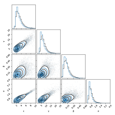
((a)) P1’ (Local Gaussian scheme)

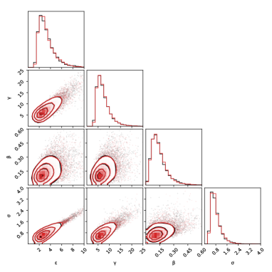
((b)) P2’ (CF-expansion with $\displaystyle J=4$)

Figure 6: Posterior estimates. P0 (benchmark posterior) is overlaid in each figure in black.

References

- Ableidinger et al. [2017] M. Ableidinger, E. Buckwar, and H. Hinterleitner. A stochastic version of the Jansen and Rit neural mass model: Analysis and numerics. J. Math. Neurosci., 7(1):1–35, 2017.
- Aït-Sahalia [2002] Y. Aït-Sahalia. Maximum likelihood estimation of discretely sampled diffusions: a closed-form approximation approach. Econometrica, 70(1):223–262, 2002.
- Aït-Sahalia [2008] Y. Aït-Sahalia. Closed-form likelihood expansions for multivariate diffusions. Ann. Statist., 36(2):906–937, 2008.
- Andrieu et al. [2010] C. Andrieu, A. Doucet, and R. Holenstein. Particle Markov chain Monte Carlo methods. J. R. Stat. Soc. Ser. B. Stat. Methodol., 72(3):269–342, 2010.
- Betancourt [2017] M. Betancourt. A conceptual introduction to Hamiltonian Monte Carlo. arXiv:1701.02434, 2017.
- Chang and Chen [2011] J. Chang and S. X. Chen. On the approximate maximum likelihood estimation for diffusion processes. Ann. Statist., 39(6):2820–2851, 2011.
- Choi [2015] S. Choi. Explicit form of approximate transition probability density functions of diffusion processes. J. Econom., 187(1):57–73, 2015.
- DeVille et al. [2005] L. DeVille, E. Vanden-Eijnden, and C. Muratov. Two distinct mechanisms of coherence in randomly perturbed dynamical systems. Phys. Rev. E, 72(3):031105, 2005.
- Ditlevsen and Samson [2019] S. Ditlevsen and A. Samson. Hypoelliptic diffusions: filtering and inference from complete and partial observations. J. R. Stat. Soc. Ser. B. Stat. Methodol., 81(2):361–384, 2019.
- Gloter and Yoshida [2021] A. Gloter and N. Yoshida. Adaptive estimation for degenerate diffusion processes. Electron. J. Stat., 15(1):1424–1472, 2021.
- Hoffman et al. [2014] M. Hoffman, A. Gelman, et al. The No-U-Turn sampler: adaptively setting path lengths in hamiltonian monte carlo. J. Mach. Learn. Res., 15(1):1593–1623, 2014.
- Iguchi and Beskos [2023] Y. Iguchi and A. Beskos. Parameter inference for hypo-elliptic diffusions under a weak design condition. arXiv:2312.04444, 2023.
- Iguchi and Yamada [2021] Y. Iguchi and T. Yamada. Operator splitting around Euler-Maruyama scheme and high order discretization of heat kernels. ESAIM: Math. Model. Numer. Anal., 55:S323–S367, 2021.
- Iguchi et al. [2024] Y. Iguchi, A. Beskos, and M. Graham. Parameter inference for degenerate diffusion processes. Stoch. Process. Their Appl., page 104384, 2024.
- Iguchi et al. [2025] Y. Iguchi, A. Beskos, and M. Graham. Parameter estimation with increased precision for elliptic and hypo-elliptic diffusions. Bernoulli, 31(1):333–358, 2025.
- Kloeden and Platen [1992] P. Kloeden and E. Platen. Numerical Solution of Stochastic Differential Equations. Springer, 1992.
- Lee et al. [2014] Y. D. Lee, S. Song, and E.-K. Lee. The delta expansion for the transition density of diffusion models. J. Econom., 178:694–705, 2014.
- Li [2013] C. Li. Maximum-likelihood estimation for diffusion processes via closed-form density expansions. Ann. Statist., 41:1350–1380, 2013.
- Li and Chen [2016] C. Li and D. Chen. Estimating jump–diffusions using closed-form likelihood expansions. J. Econom., 195(1):51–70, 2016.
- Melnykova [2020] A. Melnykova. Parametric inference for hypoelliptic ergodic diffusions with full observations. Stat. Inference Stoch. Process., 23(3):595–635, 2020.
- Nualart [2006] D. Nualart. The Malliavin Calculus and Related Topics. Springer Berlin, Heidelberg, 2006.
- Papaspiliopoulos et al. [2007] O. Papaspiliopoulos, G. Roberts, and M. Sköld. A general framework for the parametrization of hierarchical models. Stat. Sci., 22:59–73, 2007.
- Pavliotis [2014] G. Pavliotis. Stochastic Processes and Applications: Diffusion Processes, the Fokker-Planck and Langevin Equations, volume 60. Springer, 2014.
- Pigato [2022] P. Pigato. Density estimates and short-time asymptotics for a hypoelliptic diffusion process. Stoch. Process. Their Appl., 145:117–142, 2022.
- Pilipovic et al. [2024] P. Pilipovic, A. Samson, and S. Ditlevsen. Strang splitting for parametric inference in second-order stochastic differential equations. arXiv:2405.03606, 2024.
- Roberts and Stramer [2001] G. Roberts and O. Stramer. On inference for partially observed nonlinear diffusion models using the Metropolis–Hastings algorithm. Biometrika, 88(3):603–621, 2001.
- Samson et al. [2024] A. Samson, M. Tamborrino, and I. Tubikanec. Inference for the stochastic FitzHugh-Nagumo model from real action potential data via approximate Bayesian computation. arXiv:2405.17972, 2024.
- Stramer et al. [2010] O. Stramer, M. Bognar, and P. Schneider. Bayesian inference for discretely sampled Markov processes with closed-form likelihood expansions. J. Financ. Econom., 8(4):450–480, 2010.
- Vehtari et al. [2021] A. Vehtari, A. Gelman, D. Simpson, B. Carpenter, and P.-C. Bürkner. Rank-normalization, folding, and localization: An improved R̂ for assessing convergence of MCMC (with discussion). Bayesian Anal., 16(2):667–718, 2021.
- Vinga [2004] Susana Vinga. Convolution integrals of Normal distribution functions. Supplementary material to Vinga and Almeida (2004) “Rényi continuous entropy of DNA sequences”, 2004.
- Watanabe [1987] S. Watanabe. Analysis of Wiener functionals (Malliavin calculus) and its applications to heat kernels. Ann. Probab., 15(1):1–39, 1987.
- Yang et al. [2019] N. Yang, N. Chen, and X. Wan. A new delta expansion for multivariate diffusions via the Itô-Taylor expansion. J. Econom., 209(2):256–288, 2019.
- Yoshida [1992] N. Yoshida. Asymptotic expansions of maximum likelihood estimators for small diffusions via the theory of Malliavin-Watanabe. Probab. Theory Relat. Fields, 92(3):275–311, 1992.