Dimer problem on a spherical surface

Abstract

We solve the problem of a dimer moving on a spherical surface and find that its binding energy and wave function are sensitive to the total angular momentum. The dimer gets squeezed in the direction orthogonal to the center-of-mass motion and can qualitatively change its geometry from two-dimensional to one-dimensional.

The problem of two interacting bodies has a central importance in diverse areas of physics ranging from celestial mechanics and general relativity einstein1938 ; barker1975 ; buonanno1999 to classical electrodynamics schild1963 . In quantum mechanics, it underlies the solution of the hydrogen atom and the theory of scattering Landau . Two-body physics also rules the thermodynamic description of ultracold atomic gases dalfovo1999 ; giorgini2008 since their interaction range is much smaller than their de Broglie wave lengths and average interparticle distances. In particular, the zero-range scattering problem has been solved in three-dimensional free space Landau , in quasi-one-dimensional olshanii1998 and in quasi-two-dimensional petrov2001 geometries. The spectrum of a harmonically-confined pair of atoms was obtained in any spatial dimension busch1998 . In these cases, the solution of the two-body problem is simplified by its separability into two independent single-particle problems: one for the center-of-mass free dynamics, another for the relative motion of the particles.

The separability is however not assured if the particles are constrained to move in optical lattices fedichev2004 ; schneider2009 , in mixed dimensional setups massignan2006 ; nishida2008 ; lamporesi2010 ; xiao2019 , in anharmonic bolda2005 ; sala2016 or species-dependent harmonic peano2005 ; melezhik2009 potentials, or in spatial domains which are compact or curved. In particular, solving the two-body problem in curved setups is more difficult than in flat counterparts, but fundamentally valuable for discovering new quantum mechanical behaviors induced by the curved geometry tononi2023 . Indeed, the solution of one and two-body problems on a spherical surface evidenced interesting consequences associated to curvature and to non-separability. For instance, there were studies of $p$-wave dimers moving under a geometrically-induced gauge field shi2017 , of $s$-wave scattering of one body zhang2018 and of two-bodies on a large sphere tononi2022 , of the gas-to-soliton crossover tononi2024 , and of the anyonic spectrum on the sphere ouvry2019 ; polychronakos2020 . These developments address the fundamental theoretical issue of understanding few-body physics in curved geometries, and are potentially interesting for experiments with shell-shaped gases carollo2022 ; jia2022 and with other low-dimensional curved geometries fernholz2007 .

In this Letter, we calculate the ground state energy and wave function of two atoms confined to a sphere varying the scattering length $a$ and the total angular momentum $j$. Technically, at fixed $j$ the problem is reduced to a finite set of coupled differential equations for the relative wave function. We derive these equations by adapting to our case the rigid-rotor formalism of Ref. shi2017 . We find that for a small dimer, when $a$ is much smaller than $R/\sqrt{j}$ ($R$ is the sphere radius), the wave function is well approximated by the product of the isotropic relative wave function, the same as in the flat case, and the wave function of the center-of-mass motion with angular momentum $j$. However, upon increasing $a$ (or $j$) the dimer becomes anisotropic; the relative wave function gets more and more squeezed in the direction perpendicular to the direction of the center-of-mass motion. We argue that this squeezing is due to an effective harmonic confinement with oscillator length $\sim R/\sqrt{j}$ acting on the relative degree of freedom. For large $j$ our two-body problem on a sphere can be reduced to a flat-space quasi-one-dimensional problem in this effective harmonic confinement. The two-body ground state can be of localized or delocalized character and it can be two dimensional or quasi one dimensional depending on the relationships among the three relevant length scales, $a$, $R$, and $R/\sqrt{j}$. In the rest of the Letter we use the sphere radius as the unit of length, i.e., we set $R=1$.

Our findings have implications for ongoing experiments with shell-shaped magnetic guo2020 ; carollo2022 ; beregi2024 and optical jia2022 traps. In these setups one can be able to create rapidly-rotating gases by combining gravity-compensation mechanisms with phase-imprinting techniques for transferring angular momentum to the gas sharma2024 ; debussy2024 .

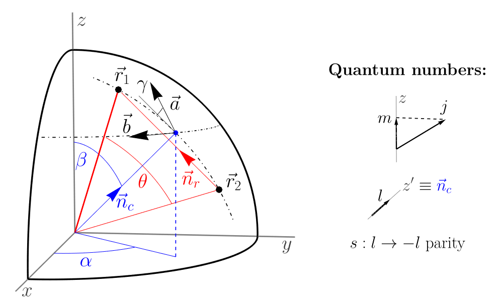
Figure 1: Illustration of the coordinate system of two particles located at $\vec{r}_{1}$ and $\vec{r}_{2}$. Their geodesic center of mass, pointed by the vector $\vec{n}_{c}$ is described by the spherical coordinates $\alpha$ and $\beta$, while their relative position, pointed by the vector $\vec{n}_{r}$, is described by the angles $\gamma$ and $\theta$. The system is characterized by four quantum numbers: the total angular momentum $j$, its projection $m$ along the axis $z$, the angular momentum $l$ describing the molecular rotation along the $z^{\prime}=\vec{n}_{c}$ axis, and the parity $s$ of the eigenstates under the exchange $l\to-l$.

Our two-body system on a sphere has four angular degrees of freedom, which admit different parametrizations. We will first work with the center-of-mass and relative angles $\vec{u}=(\alpha,\beta,\gamma,\theta)$. Figure 1 shows how the set $\vec{u}$ is related to the single-particle vectors $\vec{r}_{1}$ and $\vec{r}_{2}$ (see Appendix A for explicit expressions). The spherical coordinates $\alpha\in[0,2\pi]$ and $\beta\in[0,\pi]$ parametrize the center-of-mass vector $\vec{n}_{c}=(\vec{r}_{1}+\vec{r}_{2})/|\vec{r}_{1}+\vec{r}_{2}|$. The relative vector $\vec{n}_{r}=(\vec{r}_{1}-\vec{r}_{2})/|\vec{r}_{1}-\vec{r}_{2}|$ is parametrized by $\alpha$, $\beta$, and by the angle $\gamma\in[0,2\pi]$ between the geodesic passing by the center of mass and the great circle passing by the north pole. Finally, $\theta\in[0,\pi]$ is the relative angular distance between the atoms.

The Schrödinger equation for the two-body wave function $\Psi(\alpha,\beta,\gamma,\theta)$ reads

$$(\hat{T}-E)\Psi=0,$$ (1)

where the relation between the two-body energy $E$ and the s-wave scattering length $a$ is obtained by imposing the Bethe-Peierls boundary condition $\Psi|_{\theta\to 0}\propto\ln(\theta/a)$. The kinetic energy operator $\hat{T}$ is derived by directly calculating the Laplace-Beltrami operator in the coordinates $\vec{u}$, finding (see Appendix B for details): $\hat{T}=(\hat{J}^{2}_{x^{\prime}}/I_{x^{\prime}}+\hat{J}^{2}_{y^{\prime}}/I_{y^{\prime}}+\hat{J}^{2}_{z^{\prime}}/I_{z^{\prime}})/2+\hat{L}^{2}_{\theta}$, which is the sum of the rotational energies along the molecular axes $(\vec{x}\,^{\prime},\vec{y}\,^{\prime},\vec{z}\,^{\prime})=(\vec{n}_{r},\vec{n}_{c}\times\vec{n}_{r},\vec{n}_{c})$ and of the kinetic energy $\hat{L}^{2}_{\theta}=-(\sin\theta)^{-1}\partial_{\theta}(\sin\theta\,\partial_{\theta})$ for the relative motion along $\theta$ zhang2018 . The moments of inertia are equal to $I_{x^{\prime}}=2\cos^{2}(\theta/2)$, $I_{y^{\prime}}=2$ and $I_{z^{\prime}}=2\sin^{2}(\theta/2)$, while the expressions of the angular momentum operators $\hat{J}_{x^{\prime}}$, $\hat{J}_{y^{\prime}}$ and $\hat{J}_{z^{\prime}}$ in terms of $\alpha$, $\beta$ and $\gamma$ are reported in Appendix B. We now rewrite $\hat{T}$ through the total angular momentum operator $\hat{J}^{2}=\hat{J}_{x^{\prime}}^{2}+\hat{J}_{y^{\prime}}^{2}+\hat{J}_{z^{\prime}}^{2}$ and the ladder operators $\hat{J}_{\pm}=\hat{J}_{x^{\prime}}\pm i\hat{J}_{y^{\prime}}$, obtaining

$$\hat{T}=A(\theta)\hat{J}^{2}+B(\theta)\hat{J}^{2}_{z^{\prime}}+C(\theta)(\hat{J}_{+}^{2}+\hat{J}_{-}^{2})+\hat{L}^{2}_{\theta},$$ (2)

with $A(\theta)=[1/\cos^{2}(\theta/2)+1]/8$, $B(\theta)=[8/\sin^{2}\theta-1-3/\cos^{2}(\theta/2)]/8$ and $C(\theta)=\tan^{2}(\theta/2)/16$. The common eigenstates of $\hat{J}^{2}$ and $\hat{J}_{z^{\prime}}$ are the Wigner-D matrices $D_{ml}^{j*}(\alpha,\beta,\gamma)$ varshalovic1988 , satisfying the relations

$$\hat{J}^{2}D_{ml}^{j*} =j(j+1)D_{ml}^{j*},$$ (3)

$$\hat{J}_{z^{\prime}}^{2}D_{ml}^{j*} =l^{2}D_{ml}^{j*},$$

$$\hat{J}_{\pm}D_{ml}^{j*} =[j(j+1)-l(l\pm 1)]^{1/2}D_{ml\pm 1}^{j*}.$$

These eigenstates are labelled by the total angular momentum $j$, by its projection along the $z$ axis $m=-j,...,j$, and by the angular momentum projection along the $z^{\prime}$ axis $l=-j,...,j$ (see Fig. 1). Note that the operator $\hat{T}$ conserves $j$ and $m$, but it does couple states with $l$ different by $2$. We decompose the wave function in each $j,m$ channel as Landau ; cook

$$\Psi_{j,m}(\alpha,\beta,\gamma,\theta)=\sum_{l=0,\,\atop{l\text{ even}}}^{j}\psi_{l}(\theta)S_{jml}(\alpha,\beta,\gamma),$$ (4)

where $S_{jml}=(D_{ml}^{j*}+D_{m-l}^{j*})/\sqrt{2}$ for $l>0$, while $S_{jm0}=D_{m0}^{j*}$, and using the properties (3) we reduce Eq. (1) to

$$[\hat{L}^{2}_{\theta}+j(j+1)A(\theta)+l^{2}B(\theta)]\psi_{l}(\theta)+C(\theta)[c_{l}\psi_{l+2}(\theta)+c_{l-2}\psi_{l-2}(\theta)]=E_{j}\psi_{l}(\theta),$$ (5)

where $c_{l}=\sqrt{(j-l-1)(j-l)(j+l+1)(j+l+2)}$, $c_{0}=\sqrt{2(j-1)j(j+1)(j+2)}$, and $c_{l}=0$ for $l<0$. Note that we only include the even-$l$ wave function components in Eq. (4) because the operator $\hat{T}$ does not couple even-$l$ channels to odd-$l$ channels. Indeed, for zero-range $s$-wave interaction the odd-$l$ part describes noninteracting states and we are only interested in the even-$l$ channels (the $p$-wave-interacting case has been considered in Ref. shi2017 ). In fact, the $s$-wave interaction is effective only in the equation with $l=0$ as the other components experience the centrifugal barrier $l^{2}B(\theta)\propto 1/\theta^{2}$. Also note that $\hat{T}$ conserves parity under the exchange $l\rightarrow-l$. While the odd-parity configurations are insensitive to the interaction, the symmetric states under this exchange feel the interaction through their coupling to $\psi_{0}$. By expanding the wave function in terms of symmetric superpositions of opposite $l$ channels, $S_{jlm}$, we select only the even-parity configurations. Thus, our dimer problem with $s$-wave interaction essentially reduces to $(j+2)/2$ coupled differential equations for even $j$ or to $(j+1)/2$ equations for odd $j$ (we remind that $|l|\leq j$).

In particular, for $j=0$ we have the single equation $(\hat{L}_{\theta}^{2}-E_{0})\psi_{0}(\theta)=0$, solved in terms of Legendre functions tononi2024 : $\psi_{0}(\theta)\propto P_{-1/2+s}[\cos(\pi-\theta)]$, with $s=(E_{0}+1/4)^{1/2}$. The energy $E_{0}$ is then obtained from $\ln(1/a)=[\mathcal{D}(1/2+s)+\mathcal{D}(1/2-s)]/2+\ln(e^{\gamma_{E}}/2)$, where $\mathcal{D}$ is the digamma function and $\gamma_{E}$ is the Euler-Mascheroni constant.

The case $j=1$ is governed by a different but also single equation $[\hat{L}_{\theta}^{2}+2A(\theta)-E_{1}]\psi_{0}(\theta)=0$ which can be rewritten in the form of the generalized associated Legendre equation virchenko . We find $\psi_{0}(\theta)\propto c_{p}\mathcal{P}[\cos(\theta)]+c_{q}\mathcal{Q}[\cos(\theta)]$, where

$$\begin{split}\mathcal{P}(x)&=\sqrt{1+x}\,\,_{2}F_{1}[k+3/2,-k+1/2,1,(1-x)/2],\\ \mathcal{Q}(x)&=\frac{\sqrt{1+x}}{(x-1)^{k+3/2}}\,\,_{2}F_{1}[k+3/2,k+3/2,2k+2,2/(1-x)].\end{split}$$ (6)

are expressed in terms of the hypergeometric functions ${}_{2}F_{1}$, and the coefficients $c_{p}=-2/[\Gamma(1/2-k)\Gamma(3/2+k)]$ and $c_{q}=-i(-1)^{-k}2^{-k-1/2}\Gamma(2+2k)/\Gamma^{2}(3/2+k)$ are fixed by imposing that in $\psi_{0}$ the $(x+1)^{-1/2}$ singularities of $\mathcal{P}(x)$ and $\mathcal{Q}(x)$ at $x\rightarrow-1$ cancel out. The Bethe-Peierls boundary condition leads to the relation between the energy $E_{1}=(k+1/2)^{2}$ and the scattering length: $\ln(1/a)=\mathcal{D}(1/2+k)+1/(1+2k)-(\pi/2)\tan(\pi k)+\ln(e^{\gamma_{E}}/2)$.

For $j>1$ we solve Eqs. (5) numerically. The energies $E_{j}$ as functions of $a$ are presented in Fig. 2 as solid curves. The dashed curves correspond to the two leading-order terms in the expansion of the energy in powers of small $a$

$$E_{j}^{(a\ll 1)}=E^{(\text{flat})}-1/3+j(j+1)/4,$$ (7)

where $E^{(\text{flat})}=-4\exp(-2\gamma_{E})/a^{2}$ is the dimer energy in the flat case. The center-of-mass energy $j(j+1)/4$ and the leading-order curvature-induced shift $-1/3$ can be obtained by solving Eq. (5) perturbatively at small $\theta\sim a$. In doing this it is convenient to rewrite the operator $\hat{L}_{\theta}^{2}$ and the functions $A(\theta)$, $B(\theta)$, $C(\theta)$ changing the variable from the angle $\theta$ to the chord distance $\rho=2\sin(\theta/2)$ (see Ref. tononi2024 ). The dash-dotted horizontal lines correspond to the formulas

$$\begin{split}E_{j\,\text{even}}^{(a\gg 1)}&=j^{2}/4+j/2,\qquad\\ E_{j\,\text{odd}}^{(a\gg 1)}&=j^{2}/4+j/2+1/4.\end{split}$$ (8)

Equations (8) follow from the fact that the energy on the sphere scales quadratically with the angular momentum and, therefore, for fixed total angular momentum $j$ the lowest-energy state of two noninteracting atoms is obtained when their (integer) angular momenta $j_{1}$ and $j_{2}$ are as close as possible to $j/2$ and are also such that $j_{1}+j_{2}=j$.

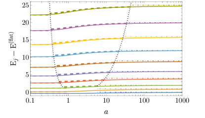
Figure 2: Dimer energy spectrum versus $a$ for $j=0,...,9$ (continuous lines). The exact curves converge towards the analytical asymptotes of Eqs. (7) and (8) valid, respectively, in the strongly-attractive regime $a\ll 1$ (dashed lines), and in the noninteracting regime $a\gg 1$ (dot-dashed lines). In the intermediate $a$ regime, the curves are well reproduced by the semianalytical quasi-one-dimensional theory (thick dashed lines). The dimer is quasi-one-dimensional between the dotted curves; the left border corresponds to the dimer aspect ratio $\sim 1$ and the right border indicates where the dimer size becomes comparable to the sphere radius (see text).

We now discuss how the wave function depends on $j$. For $j=0$ and $j=1$ only $\psi_{0}$ is nonzero and the total wave function is independent of $\gamma$, which can be seen from Eq. (4) bearing in mind that $S_{000}=1$ and $S_{110}=e^{-i\alpha}\sin\beta/\sqrt{2}$. The dimer in these cases is isotropic although the $\theta$ dependence of its wave function is sensitive to $j$. The anisotropy first appears in the case $j=2$ where $\psi_{2}\neq 0$. It manifests itself in a squeezing of the molecule along a direction which depends on the center-of-mass angles $\alpha$ and $\beta$ and on $m$ (note, however, that $\psi_{l}$ depend on $j$, but not on $m$). The phenomenon can be seen clearly in the case $m=j$, which corresponds to the center-of-mass motion of the molecule along the equator. If we also set the center of mass on the equator ($\beta=\pi/2$), the wave function (4) explicitly reads $\Psi_{j,j}(\alpha,\pi/2,\gamma,\theta)\propto e^{-ij\alpha}\sqrt{(2j)!}[\psi_{0}(\theta)/j!+\sum_{l>0}\psi_{l}(\theta)\cos(l\gamma)/\sqrt{2(j+l)!(j-l)!}]/2^{j}$. We demonstrate the squeezing of the dimer by plotting the quantity $|\Psi_{j,j}(\alpha,\pi/2,\gamma,\theta)/\Psi^{\rm(flat)}(\theta)|$ in Fig. 3 for $a=2$ (note that $|\Psi_{j,j}(\alpha,\pi/2,\gamma,\theta)|$ is independent of $\alpha$). We divide by the (isotropic) bound-state wave function in the flat-case limit $\Psi^{\rm(flat)}(\theta)=K_{0}(2e^{-\gamma_{E}}\theta/a)$ to remove the logarithmic divergence at $\theta\to 0$ and to better visualize the angular distribution of the state. We observe that by increasing $j$ the dimer becomes more and more squeezed in the direction perpendicular to the equator, i.e., perpendicular to the center-of-mass motion.

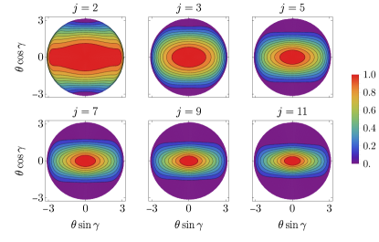
Figure 3: Contour plots of the ratio (rescaled to its maximum) $|\Psi_{j,m}(\alpha,\pi/2,\gamma,\theta)/K_{0}(2e^{-\gamma_{E}}\theta/a)|$ for $a=2$, which demonstrate the squeezing of the state along the direction of motion of the center of mass.

The squeezing becomes more pronounced for large $j$. In this case the dimer wave function (4) involves many $l$-components and for describing the system it is more convenient to switch from $(\alpha,\beta,\gamma,\theta)$ to the single-particle bases of polar and azimuthal angles $(\theta_{1},\phi_{1},\theta_{2},\phi_{2})$. As we have already mentioned, for fixed $j$ (let us assume for simplicity that $j$ is even), two non-interacting atoms prefer to occupy single-particle orbitals with angular momenta $j_{1}=j_{2}=j/2$. If $m=j$, we also have $m_{1}=m_{2}=j/2$. For large $j$ such orbitals are localized close to the equator of the sphere where $\theta_{\sigma}\approx\pi/2$. The variation of $\theta_{\sigma}$ is of order $|\theta_{\sigma}-\pi/2|\sim 1/\sqrt{j}$. One can see this by switching to the variable $y_{\sigma}=\theta_{\sigma}-\pi/2$ and observing that the single-particle kinetic energy operator can be written as $[-\partial^{2}/\partial y_{\sigma}^{2}+\tan y_{\sigma}\partial/\partial y_{\sigma}+j^{2}/(4\cos^{2}y_{\sigma})]/2$. The expansion of $j^{2}/8\cos^{2}y_{\sigma}$ at small $y_{\sigma}$ gives an approximately harmonic potential with frequency $j/2$ which localizes the wave function to the oscillator length $\sqrt{2/j}$. As we show in Appendix C this localization persists also in the interacting case. The dimer problem becomes quasi-one-dimensional and the dimer energy $E=j^{2}/4+j/2+q^{2}$ is obtained by solving

$$\int_{0}^{\infty}e^{2q^{2}\tau/j}\left(\sqrt{\tau/\sinh\tau}e^{\tau/2}-1\right)\frac{d\tau}{4\pi\tau}=\frac{1}{2\pi}\ln\frac{\sqrt{-q^{2}}ae^{\gamma_{E}}}{2}.$$ (9)

The corresponding results are shown as dashed curves in Fig. 2. Equation (9) is valid for $j=m\gg 1$ and we require $1\ll-q^{2}\lesssim j$ (see more details in Appendix C). Under these conditions the two-body wave function is well approximated by $\Psi(\theta_{1},\phi_{1},\theta_{2},\phi_{2})\approx\exp[-j(\theta_{1}-\pi/2)^{2}/4-j(\theta_{2}-\pi/2)^{2}/4-\sqrt{-q^{2}}|\phi_{1}-\phi_{2}|]$, its quasi-one-dimensional character is explicit; in the direction of the center-of-mass motion the dimer has the size $1/\sqrt{-q^{2}}$ which is larger than its width given by $\sim 1/\sqrt{j}$.

We can now summarize the main regimes of an $s$-wave-interacting dimer on a sphere. For small $j$, with increasing $a$ the dimer increases in size, but remains to a large extent isotropic. The change of the character in this case happens at $a\sim 1$ when the dimer size becomes comparable to the sphere radius. For large $j$ we identify the following three regimes. For $a\lesssim 1/\sqrt{j}$ the dimer is strongly bound and approximately isotropic. In the interval $1/\sqrt{j}\lesssim a\lesssim a^{*}$ the dimer is quasi-one-dimensional and its size is smaller than the sphere radius. The characteristic scattering length $a^{*}\approx e^{\sqrt{\pi j/2}}$ is obtained by setting $q^{2}=-1$ in Eq. (9). It marks the crossover to the third regime where the two atoms are delocalized along the equator, but localized in the perpendicular direction with polar angles $|\theta_{\sigma}-\pi/2|\sim 1/\sqrt{j}$. The dotted curves in Fig. 2 correspond to $a=1/\sqrt{j}$ (left border) and $a=a^{*}$ (right border) and indicate the regime where the dimer is quasi-one-dimensional.

In conclusion, we find the spectrum and wave functions of an $s$-wave-interacting dimer on a spherical surface as a function of the scattering length $a$ and total angular momentum $j$. The nonseparability of the relative and center-of-mass degrees of freedom manifests itself in squeezing of the dimer in the direction transversal to the center-of-mass motion. The effect is most pronounced for $a\gtrsim 1/\sqrt{j}$ when the dimer becomes quasi-one-dimensional. Moreover, for $a\gg 1$, when the attraction is insufficient to localize two atoms into a dimer at low $j$, this transversal squeezing enhances the attraction and eventually leads to a bound quasi-one-dimensional dimer at sufficiently large $j$.

Future experiments with shell-shaped bosons in magnetic carollo2022 or optical jia2022 traps may soon be able to combine the two-dimensional confinement with phase imprinting techniques to rotate the gas, opening the way to the observation of this phenomenon and its consequences.

*

Appendix A Appendix A: Particle positions in $\vec{u}$ coordinates

The particle positions $\vec{r}_{1}$ and $\vec{r}_{2}$ can be expressed in terms of $\vec{n}_{c}$ and $\vec{n}_{r}$ as

$$\begin{split}\vec{r}_{1}&=\vec{n}_{c}\cos(\theta/2)+\vec{n}_{r}\sin(\theta/2),\\ \vec{r}_{2}&=\vec{n}_{c}\cos(\theta/2)-\vec{n}_{r}\sin(\theta/2),\end{split}$$ (10)

where the geodesic center-of-mass and relative vectors are respectively given by $\vec{n}_{c}=(\sin\beta\cos\alpha,\sin\beta\sin\alpha,\cos\beta)^{T}$ and $\vec{n}_{r}=\cos\gamma\,\vec{a}+\,\sin\gamma\,\vec{b}$. In particular, see Fig. 1, $\vec{a}=(-\cos\beta\cos\alpha,-\cos\beta\sin\alpha,\sin\beta)^{T}$ is the tangent vector to the center of mass directed along the great circle passing by the north pole, while $\vec{b}=(\sin\alpha,-\cos\alpha,0)^{T}$ is the tangent vector to the center of mass directed along the circle parallel to the equator. Given the above relations, Eq. (10) represents the particles positions in terms of the angles $\vec{u}$.

The body-fixed frame is built on the basis vectors $\vec{n}_{r}$, $\vec{n}_{c}\times\vec{n}_{r}$, and $\vec{n}_{c}$, which define the $x^{\prime}$, $y^{\prime}$, and $z^{\prime}$ axes, respectively. The transition from the space-fixed to body-fixed frame is carried out with the help of the rotation matrix $\mathcal{R}=(\vec{n}_{r},\vec{n}_{c}\times\vec{n}_{r},\vec{n}_{c})$ such that any vector $\vec{r}\,^{\prime}=(x^{\prime},y^{\prime},z^{\prime})^{T}$ defined in the body-fixed frame corresponds to ${\vec{r}}=\mathcal{R}\,\vec{r}\,^{\prime}$ in the laboratory frame. For instance, the particles coordinates correspond to $\vec{r_{1}}\,^{\prime}=(\sin(\theta/2),0,\cos(\theta/2))^{T}$ and $\vec{r_{2}}\,^{\prime}=(-\sin(\theta/2),0,\cos(\theta/2))^{T}$.

Appendix B Appendix B: Kinetic energy in $\vec{u}$ coordinates

The kinetic energy operator can be expressed in terms of the angles $\vec{u}=(\alpha,\beta,\gamma,\theta)$ by calculating the Laplace-Beltrami operator

$$\hat{T}=-\frac{1}{2}\frac{1}{\sqrt{g}}\partial_{i}(\sqrt{g}g^{ij}\partial_{j}),$$ (11)

where $\partial_{i}=\partial/\partial u^{i}$, $g=\det(g_{ij})$, and $g^{ij}$ is the inverse of the metric tensor $g_{ij}$, defined through the line element squared $ds^{2}$ as $ds^{2}=(d\vec{r}_{1})^{2}+(d\vec{r}_{2})^{2}=g_{ij}\,du^{i}du^{j}$. Thus, by differentiating the coordinates at Eq. (10) in terms of the angles $\vec{u}$, we obtain the metric tensor

$$g_{ij}=\begin{bmatrix}h_{ij}&\vec{0}\\ \vec{0}&1/2\end{bmatrix},$$ (12)

with $g=\sin^{2}\beta\sin^{2}\theta$, and where the symmetric $3\times 3$ tensor $h$ has components

$$\begin{split}h_{11}=&2\sin^{2}\beta[\cos^{2}\gamma+\cos^{2}(\theta/2)\sin^{2}\gamma-\sin^{2}(\theta/2)\cos(2\gamma)]+\\ &2\sin^{2}(\theta/2)\cos^{2}\beta,\\ h_{12}=&2\sin^{2}(\theta/2)\sin\beta\sin\gamma\cos\gamma,\\ h_{13}=&2\sin^{2}(\theta/2)\cos\beta,\\ h_{22}=&2\sin^{2}\gamma+2\cos^{2}(\theta/2)\cos^{2}\gamma+2\sin^{2}(\theta/2)\cos(2\gamma),\\ h_{23}=&0,\\ h_{33}=&2\sin^{2}(\theta/2).\end{split}$$ (13)

We calculate Eq. (11) explicitly and obtain the kinetic energy operator presented in the main text $\hat{T}=(\hat{J}^{2}_{x^{\prime}}/I_{x^{\prime}}+\hat{J}^{2}_{y^{\prime}}/I_{y^{\prime}}+\hat{J}^{2}_{z^{\prime}}/I_{z^{\prime}})/2+\hat{L}^{2}_{\theta}$, whose angular momentum components are defined as

$$\begin{split}\hat{J}_{x^{\prime}}&=i\bigg{(}\frac{\cos\gamma}{\sin\beta}\partial_{\alpha}-\sin\gamma\partial_{\beta}-\cot\beta\cos\gamma\partial_{\gamma}\bigg{)},\\ \hat{J}_{y^{\prime}}&=i\bigg{(}-\frac{\sin\gamma}{\sin\beta}\partial_{\alpha}-\cos\gamma\partial_{\beta}+\cot\beta\sin\gamma\partial_{\gamma}\bigg{)},\\ \hat{J}_{z^{\prime}}&=-i\partial_{\gamma},\end{split}$$ (14)

in the molecular frame.

For completeness, we report the orthogonality relation of the Wigner-D functions used in the main text for projecting the Schrödinger equation varshalovic1988

$$\begin{split}&\int_{0}^{2\pi}d\alpha\int_{0}^{\pi}d\beta\sin\beta\int_{0}^{2\pi}d\gamma D_{m^{\prime}l^{\prime}}^{j^{\prime}*}(\alpha,\beta,\gamma)D_{ml}^{j}(\alpha,\beta,\gamma)\\ &=\frac{8\pi^{2}}{2j+1}\delta_{jj^{\prime}}\delta_{mm^{\prime}}\delta_{ll^{\prime}}.\end{split}$$

Appendix C Appendix C: Derivation of Eq. (9)

In this appendix we discuss the case $j=m\gg 1$. Let us write the two-body wave function in the form $\Psi(\theta_{1},\phi_{1},\theta_{2},\phi_{2})=\chi(y_{1},y_{2},x)e^{ij\phi_{c}}$, where $y_{\sigma}=\theta_{\sigma}-\pi/2$ is the deviation from the equator, $x=\phi_{1}-\phi_{2}$, $\phi_{c}=(\phi_{1}+\phi_{2})/2$, and $j$ is large integer, even or odd. The Schrödinger equation without interaction (1) in these coordinates becomes

$$\begin{split}\sum_{\sigma=1,2}\left[-\frac{1}{2}\frac{\partial^{2}}{\partial y_{\sigma}^{2}}+\frac{\tan y_{\sigma}}{2}\frac{\partial}{\partial y_{\sigma}}+\frac{1}{\cos^{2}y_{\sigma}}\left(\frac{j^{2}}{8}-\frac{1}{2}\frac{\partial^{2}}{\partial x^{2}}\right)\right]\chi\\ -\frac{j}{2}\left(\frac{1}{\cos^{2}y_{1}}-\frac{1}{\cos^{2}y_{2}}\right)i\frac{\partial}{\partial x}\chi=E\chi.\end{split}$$ (15)

The interaction is taken into account via a Bethe-Peierls boundary condition at $\{x,y_{1}-y_{2}\}={\bf 0}$. Let us assume (and a posteriori verify) that $y_{\sigma}\sim 1/\sqrt{j}$, $\partial/\partial y_{\sigma}\sim\sqrt{j}$, and that $\partial/\partial x$ is at most of order $\sqrt{j}$. Then, keeping only terms $\sim j^{2}\chi$ and $j\chi$ Eq. (15) reduces to

$$\left(-\frac{1}{4}\frac{\partial^{2}}{\partial Y^{2}}+\frac{j^{2}}{4}Y^{2}-\frac{\partial^{2}}{\partial y^{2}}+\frac{j^{2}}{16}y^{2}-\frac{\partial^{2}}{\partial x^{2}}+\frac{j^{2}}{4}\right)\chi=E\chi$$ (16)

with $y=y_{1}-y_{2}$ and $Y=(y_{1}+y_{2})/2$. We thus arrive at the problem of two atoms of unit mass trapped in the $y$ direction by a harmonic potential with frequency $j/2$. As we mention in the main text this confinement arises from the expansion of the term $j^{2}/(8\cos^{2}y_{\sigma})$ in Eq. (15) in powers of $y_{\sigma}$. It reflects the centrifugal barrier felt by the atoms as they deviate from the equator trying to approach any of the poles.

Equation (16) is supplemented by the periodicity condition $\chi(Y,x,y)=(-1)^{j}\chi(Y,2\pi+x,y)$ and by the Bethe-Peierls constraint on the asymptotic behavior of the wave function $\chi(Y,x\rightarrow 0,y\rightarrow 0)\propto\ln[(x^{2}+y^{2})/a^{2}]$. The center-of-mass motion separates from the relative one: $\chi(Y,x,y)=e^{-jY^{2}/2}\tilde{\chi}(x,y)$. The relative wave function $\tilde{\chi}$ can be written in the form of the Green function of a harmonic oscillator feynman1965 adapted to satisfy the periodicity condition

$$\tilde{\chi}(x,y)=\sum_{n=-\infty}^{\infty}\!(-1)^{jn}\!\int_{0}^{\infty}\frac{e^{-y^{2}\frac{\coth\tau}{4l_{\perp}^{2}}+q^{2}l_{\perp}^{2}\tau+\frac{\tau}{2}-\frac{(x+2\pi n)^{2}}{4\tau l_{\perp}^{2}}}}{4\pi\sqrt{\tau\sinh\tau}}d\tau,$$ (17)

where $l_{\perp}=\sqrt{2/j}$ is the oscillator length. The total energy $E=j^{2}/4+j/2+q^{2}$ decomposes into the kinetic energy of the center-of-mass motion along the equator ($j^{2}/4$), the center-of-mass zero-point energy along $y$ ($j/4$), the relative zero-point energy ($j/4$), and the energy of the relative motion along $x$ which we denote by $q^{2}$.

We now establish the relation between $q^{2}$ and $a$ applying the Bethe-Peierls constraint, which is sufficient to write as $\tilde{\chi}(x,0)\propto\ln(x/a)$. Adding and subtracting the logarithmically diverging part from Eq. (17) and then setting $x=0$ in the nondiverging terms gives

$$\tilde{\chi}(x,0)=F_{1}(x)+F_{2}+F_{3}+o(x^{0}),$$ (18)

where

$$\begin{split}F_{1}(x)&=\int_{0}^{\infty}e^{q^{2}l_{\perp}^{2}\tau-x^{2}/(4\tau l_{\perp}^{2})}\frac{d\tau}{4\pi\tau}=K_{0}(\sqrt{-q^{2}l_{\perp}^{2}}x)/(2\pi)\\ &=-\ln(\sqrt{-q^{2}x^{2}}e^{\gamma_{E}}/2)/(2\pi)+o(x^{0}),\end{split}$$ (19)

$$F_{2}=\int_{0}^{\infty}e^{q^{2}l_{\perp}^{2}\tau}\left(\sqrt{\tau/\sinh\tau}e^{\tau/2}-1\right)\frac{d\tau}{4\pi\tau},$$ (20)

and

$$\begin{split}F_{3}&=\sum_{n=-\infty,n\neq 0}^{\infty}\!(-1)^{jn}\!\int_{0}^{\infty}\frac{e^{q^{2}l_{\perp}^{2}\tau+\frac{\tau}{2}-\frac{(2\pi n)^{2}}{4\tau l_{\perp}^{2}}}}{4\pi\sqrt{\tau\sinh\tau}}d\tau\\ &\approx\frac{1}{[e^{2\pi\sqrt{-q^{2}}}-(-1)^{j}]\sqrt{-2\pi q^{2}l_{\perp}^{2}}}.\end{split}$$ (21)

In Eq. (21) we use the fact that the main contribution to the integral comes from $\tau\sim 1/l_{\perp}^{2}\gg 1$. Then, approximating $\sinh\tau\approx e^{\tau}/2$ the integral and the sum in Eq. (21) can be calculated analytically. The relation between $q$ and $a$ is obtained by noting that according to the Bethe-Peierls condition Eq. (18) should behave as $-\ln(x/a)/(2\pi)$ at small $x$. In this manner we obtain

$$\begin{split}\int_{0}^{\infty}e^{q^{2}l_{\perp}^{2}\tau}\left(\sqrt{\tau/\sinh\tau}e^{\tau/2}-1\right)\frac{d\tau}{4\pi\tau}\\ +\frac{1}{[e^{2\pi\sqrt{-q^{2}}}-(-1)^{j}]\sqrt{-2\pi q^{2}l_{\perp}^{2}}}=\frac{1}{2\pi}\ln\frac{\sqrt{-q^{2}}ae^{\gamma_{E}}}{2}.\end{split}$$ (22)

We now discuss validity of Eq. (22). When the distance between the two atoms is larger than $l_{\perp}$, i.e., when $|x+2\pi n|\gtrsim 1/\sqrt{j}$ (for any integer $n$), the wave function $\chi$ behaves as

$$\chi(Y,x,y)\propto e^{-jY^{2}/2-jy^{2}/8}\sum_{n}(-1)^{nj}e^{-\sqrt{-q^{2}}|x+2\pi n|}.$$ (23)

We derive Eq. (23) from Eq. (17) by using the approximations $\coth\tau\approx 1$ and $\sinh\tau\approx e^{\tau}/2$ valid since typical $\tau$ are large. We see that the characteristic length scale for the variation of $\chi$ in the $y$ direction is indeed $\sim 1/\sqrt{j}$ and the characteristic length scale in the $x$ direction is $1/|q|$. This verifies that Eq. (16) is valid for $|q|\sim\partial/\partial x\lesssim\sqrt{j}$ as we initially assumed.

We remind that passing from Eq. (15) to Eq. (16) we kept only terms of order $j^{2}$ and $j$. Therefore, in principle, we should not allow $|q^{2}|$ to be smaller than $j$ in order not to exceed the accuracy of the approximation. However, considering the difference between Eqs. (16) and (15) as the perturbation and Eq. (23) as the unperturbed solution to the Harmonic problem Eq. (16), one can show that the first-order and higher-order energy shifts are of order ${\rm max}\{q^{2},1\}/j$. We can thus claim that Eq. (22) also makes sense for $q^{2}\sim 1$ and can describe the whole crossover from the isotropic molecule ($|q|\sim\sqrt{j}$) to the noninteracting limit $a\rightarrow\infty$ where it correctly reproduces Eqs. (8) predicting $q^{2}=0$ for even $j$ and $q^{2}=1/4$ for odd $j$. To solve Eq. (22) for positive $q^{2}$ we use analytical continuation.