HoneyComb: A Parallel Worst-Case Optimal Join on Multicores

Abstract.

To achieve true scalability on massive datasets, a modern query engine needs to be able to take advantage of large, shared-memory, multicore systems. Binary joins are conceptually easy to parallelize on a multicore system; however, several applications require a different approach to query evaluation, using a Worst-Case Optimal Join (WCOJ) algorithm. WCOJ is known to outperform traditional query plans for cyclic queries. However, there is no obvious adaptation of WCOJ to parallel architectures. The few existing systems that parallelize WCOJ do this by partitioning only the top variable of the WCOJ algorithm. This leads to work skew (since some relations end up being read entirely by every thread), possible contention between threads (when the hierarchical trie index is built lazily, which is the case on most recent WCOJ systems), and exacerbates the redundant computations already existing in WCOJ.

We introduce HoneyComb, a parallel version of WCOJ, optimized for large multicore, shared-memory systems. HoneyComb partitions the domains of all query variables, not just that of the top loop. We adapt the partitioning idea from the HyperCube algorithm, developed by the theory community for computing multi-join queries on a massively parallel shared-nothing architecture, and introduce new methods for computing the shares, optimized for a shared-memory architecture. To avoid the contention created by the lazy construction of the trie-index, we introduce CoCo, a new and very simple index structure, which we build eagerly, by sorting the entire relation. Finally, in order to remove some of the redundant computations of WCOJ, we introduce a rewriting technique of the WCOJ plan that factors out some of these redundant computations. Our experimental evaluation compares HoneyComb with several recent implementations of WCOJ.

1. Introduction

To achieve true scalability on massive datasets, a modern query engine needs to be able to take advantage of large, shared-memory, multicore systems. Cloud companies offer servers with dozens of cores and many terabytes of main memory; for example systems with up to 224 physical cores and 24TB of main memory are available on AWS (AWS, 2024). Users who need to perform complex data analytics on large datasets will likely use such large servers for their needs, and expect the query engine to scale up. The research community has studied parallel algorithms for query processing extensively for over three decades, initially with a focus on shared-nothing architectures (DeWitt et al., 1990; DeWitt and Gray, 1990, 1992; DeWitt et al., 1992), but also on the shared-memory, multicore architectures that are the focus of this paper (Boncz and Kersten, 1999; Blanas et al., 2011; Zhang et al., 2019; Shahvarani and Jacobsen, 2020; Zhang et al., 2021, 2021; Wu et al., 2022). Many modern database engines use multi-threads during query evaluation, and thus are prepared to use multiple cores, when they are available.

Binary joins are conceptually easy to parallelize on a multicore system: both relations are hash-partitioned, then the join is computed in parallel in each partition. Practical challenges consist of reducing the number of blocking steps, reducing the number of cache misses, and reducing the overhead of locks. There exist several solutions for these challenges, see for example the excellent discussion in (Blanas et al., 2011).

However, applications like graph databases, social network analysis, RDF/Sparql engines, queries on knowledge graphs, and even sparse tensor compilers, are using a different approach to compute multi-join queries, called Worst-Case Optimal Join, WCOJ (Veldhuizen, 2014; Brisaboa et al., 2015; Chu et al., 2015; Aberger et al., 2016; Freitag et al., 2020a; Arroyuelo et al., 2021; Wang et al., 2023b; Salihoglu, 2023; Jin et al., 2023). The WCOJ algorithms are theoretically optimal, and are known to outperform binary joins on cyclic queries (but not on acyclic ones), making them well-suited for these specialized engines and even for some general-purpose relational engines (Aref et al., 2015; Freitag et al., 2020a).

Unfortunately, there is no obvious adaptation of a parallel hash-partitioned binary join to WCOJ. Unlike a traditional query plan, a WCOJ algorithm joins all relations at once. The algorithm consists of several nested loops, with one iteration for each join variable of the query. There exist a few parallel implementations of WCOJ, and they parallelize only the topmost loop. For example both LogicBlox (Aref et al., 2015) and Umbra (Freitag et al., 2020a) , as well as its Diamond-hardened extension (Birler et al., 2024), adopt this simple parallelization strategy. Under this approach, the system hash-partitions the domain of the topmost variable into sets of equal size, then executes the query for each partition in a separate logical thread. Each thread executes the remaining loops of the WCOJ sequentially. As a consequence, while each thread reads only a small fragment of the relations that contain the first iteration variable, it reads and processes the other relations entirely. In other words, relations that do not contain the top-most variable are not partitioned at all under this approach.

Listing A: Original Query

⬇

Q := R(X,Y), S(Y,Z), T(Z,X)

For x $\in$ R.X $\cap$ T.X

For y $\in$ R[x].Y $\cap$ S.Y

For z $\in$ S[y].Z $\cap$ T[x].Z

Q += (x, y, z)

Listing B: Traditional Parallelization

⬇

// Parititon R.X and T.X on X

// In parallel, Thread i:

For x $\in$ R_ii.X $\cap$ T_ii.X

For y $\in$ R_ii[x].Y $\cap$ S.Y

For z $\in$ S[y].Z $\cap$ T_ii[x].Z

Q += (x, y, z)

Listing C: HoneyComb’s Parallelization

⬇

// Partition R, S and T (see text)

// In parallel, Thread (i, j, k)

For x $\in$ R_iij.X $\cap$ T_iik.X

For y $\in$ R_iij[x].Y $\cap$ S_ijk.Y

For z $\in$ S_ijk[y].Z $\cap$ T_iik[x].Z

Q += (x, y, z)

Figure 1. Comparison of WCOJ Parallelization Algorithms

In this paper, we introduce HoneyComb, a parallel version of WCOJ, optimized for large multicore, shared-memory systems. HoneyComb partitions the domain of every variable, not just the top-most variable, and creates a separate thread for every combination of partitions. This idea has been originally proposed for shared-nothing architectures, first for MapReduce systems (Afrati and Ullman, 2010), then was studied extensively under a theoretical model of computation called Massively Parallel Communication (MPC) model, where the algorithm is known as the HyperCube Algorithm (Beame et al., 2017; Koutris et al., 2016, 2018; Hu and Yi, 2020; Hu, 2021).

HoneyComb overcomes three limitations of the traditional WCOJ parallelization method: load skew, work duplication, and contention due to lazy index creation. We start by illustrating the first limitation of the traditional method, load skew, using an example.

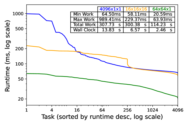
Figure 2. Skewness for Triangle Query on WGPB. Here each of the three lines represents the same number of partitions, $4096$, but allocated differently to the three attributes $X$, $Y$, and $Z$. The expression $4096\times 1\times 1$ (the blue line) means that the attribute $X$ was partitioned into $4096$ buckets and assigned to the threads, while the attributes $Y$, $Z$ were not partitioned (or partitioned into $1$ bucket). Similarly, $16\times 16\times 16$ (the orange line) means that each of $X$, $Y$, $Z$ was partitioned into $16$ buckets, for a total of $4096$ buckets/threads. Each point in the graph represents the runtime of one of the $4096$ threads, run in isolation, on one core; when executed on all $60$ cores, these threads will be dynamically scheduled on all $60$ cores, using work stealing.

Example 1.1.

Listing A in Fig. 1 illustrates WCOJ with the triangle query $Q(X,Y,Z)=R(X,Y),S(Y,Z),T(Z,X)$. We ran this query on the (undirected) WGPB (wgp, 2019; Hogan et al., 2019) dataset, with $54.0$M nodes and $81.4$M edges, using 4096 threads on a server with 60 physical cores and 120 hyperthreads. The traditional way to parallelize this query is shown in Listing B. The domain of the first variable, $X$, is partitioned into 4096 fragments. This partitions $R(X,Y)$ and $T(Z,X)$, but does not partition $S(Y,Z)$. Each thread $i=1,2,\ldots,4096$ reads only a $1/4096$-fragment of $R$ and $T$, but reads the entire relation $S$. We instrumented the code to measure, for each thread, its runtime: we show their distribution as the blue line in Fig. 2. The skew (ratio between the largest and smallest runtime) is quite visible, showing a factor of more than 15. The cumulative time of the 4096 threads, i.e. the area under the curve, is 308s. We used standard work-stealing to execute the threads on the 60 cores, thus, in an ideal scenario the total runtime should be $308/60=5.13$s: however, the actual measured total runtime (shown in the table at the top left) was 13.83s. As we will see, the discrepancy is mostly due to skew.

Instead of the traditional parallelization technique, HoneyComb partitions all query variables.

We illustrate this with an example.

Example 1.2.

Listing C in Fig. 1 shows how HoneyComb executes the triangle query, by partitioning each variable domain. On the MPC model, the theoretically optimal partitioning is $16\times 16\times 16$, meaning that the domain of each variable $X,Y,Z$ is hash-partitioned into 16 buckets. A thread is identified by a triple $(i,j,k)$, where each of $i,j,k$ range from $1$ to $16$, and it will only read a fragment of $1/16^{2}=1/256$ of each relation $R,S,T$. The runtime distribution is the orange line in Fig. 2. The total work performed by the 4096 threads (area under the curve) was $300$s, almost identical to the traditional method (Example 1.1). But the skew ratio is only about 4, and the actual measured runtime on 60 cores decreased to 6.57s. By reducing the load skew, HoneyComb reduced runtime by $2\times$.

The second limitation of the traditional approach is work duplication. For example, referring to Listing B, the fragment $S[y]$ of the relation $S$ needs to be accessed by all 4096 threads in order to perform the intersection $S[y].Z\cap T_{i}[x].Z$. In order to reduce or to eliminate redundant work, HoneyComb departs from the theoretical MPC model, because the optimal partitioning strategy of the MPC model may also lead to work duplication. For example, in Listing C, the fragment $R_{ij}[x]$ of the relation $R$ needs to be accessed by all 16 threads $k=1,2,\ldots,16$ in order to perform the intersection $R_{ij}[x].Y\cap S_{jk}.Y$.

One contribution in HoneyComb is a novel cost-based optimization of the number of buckets allocated to each variable, called the share of that variable.

While the problem of computing optimal shares has been extensively studied by the MPC model, their solutions do not carry over to multicores. The reason is that in the MPC model the communication is separated from the computation, and the optimal shares minimize only the communication cost, ignoring any work duplication at the servers. In a shared-memory system there is no communication cost, instead the total work becomes the main cost. HoneyComb computes the optimal shares using a cost model, which aims to minimize both skew and work duplication.

Example 1.3.

The problem in the previous example is that, by partitioning the last variable $Z$, we create duplicated work for intersections of the previous variables. Two threads with identifiers $(i,j,k_{1})$ and $(i,j,k_{2})$ will see exactly the same partition $R_{ij}$. In addition, if the data is dense, then they will likely also see similar values in $T_{ik}.X$, $S_{jk}.Y$. This causes portions of the top loops to be executed redundantly by different threads. The choice of how many shares to allocate for each variable depends on the data distribution. In our example, HoneyComb choose as optimal shares $64\times 64\times 1$. The load distribution for these shares is the green line in Fig. 2, and the cumulative load of all 4096 threads (area under the curve) has decreased to $114$s, from about $300$s for the $4096\times 1\times 1$ and the $16\times 16\times 16$ shares. As a consequence, the actual measured runtime on 60 cores decreased to $2.46$s.

We introduced a novel cost model specifically for shared-memory, parallel WCOJ, based on a pessimistic cardinality estimator (Cai et al., 2019), more precisely on a recent refinement (Khamis et al., 2024) that uses more sophisticated statistics on the input relations rather than just their cardinalities. To the best of our knowledge this is the first cost model proposed for WCOJ. Our cost model is described in Sec. 6.2.

Finally, the third limitation of the traditional approach comes a particular optimization in modern WCOJ systems, the lazy construction of the hash-trie, which in the parallel setting leads to contention between threads.

All WCOJ implementations index the data, in order to speed up the intersections that need to be done at each iteration of the algorithm. While a standard trie was used in an early implementation of WCOJ (Veldhuizen, 2014), recent implementations use a hash trie index. For each relation, the first level of the trie is a hash table consisting of values of the first variable, pointing to hash tables consisting of values of the second variable, and so on. Since the hash trie construction is expensive, recent systems compute lazily the entries on levels two and higher: only sub-tries that are actually needed are constructed (Freitag et al., 2020a; Wang et al., 2023b). We illustrate this in Fig. 3, where the lazy sub-trie construction applies to $R.Z$ and $T.Z$. However, when done in parallel, the lazy index requires all index accesses to be coordinated via locks, in order to avoid read-write conflicts. This is not a problem for a small number of cores, say 12-16, but it becomes a problem for a larger number of cores, which is our target for HoneyComb.

To avoid this contention and further remove the need for locks, HoneyComb introduces a new, and simple sort-based trie index that we call Compressed Column layout, or CoCo. Level $k$ of CoCo is a sorted array, consisting of the first $k$ attributes of the relation, which pointers to the next level of the trie. We construct CoCo eagerly, by first sorting the entire relation once, then computing each level by a projection and duplication elimination. We benefit from the fact that there exists very effective parallel, shared-memory sorting algorithm: HoneyComb uses ips4o (In-place Parallel Super Scalar Samplesort) (Axtmann et al., 2017, 2020) for this purpose. By replacing the hash-based index with a sort-based one we reduce the construction time significantly, and this allows us to compute it eagerly, and avoiding any need for coordination during the parallel execution of WCOJ. Thus, CoCo represents a return to the original trie in LFTJ (Veldhuizen, 2014), but in a simplified form, where the entire level $k$ is a single array, which allows us to construct the entire index using a single parallel sort.

Finally, a last challenge of the WCOJ algorithm that we observed in HoneyComb is that it some duplicated work can be avoided by storing intermediate results and using them later. Each loop of a WCOJ computes the intersection of all domains of the current variable. Some of these intersections are computed repeatedly, for different iterations of some outer loop. This occurs in both sequential and parallel implementations of WCOJ, but it seems to impact more the parallel implementation. To address that, we introduce an optimization that we call a rewriting mechanism. We precompute this intersection during the outer loop, then take advantage of the shared memory that allows multiple threads to read that intermediate result. We describe the rewriting mechanism in Sec. 6.1.

We have evaluated our methods and compared them with the state-of-the-art parallel implementations of WCOJ. Our approach, HoneyComb, demonstrates strong scalability, achieving near-linear scaling observed up to 60 cores. HoneyComb outperforms other baselines by 3x on the WGPB dataset, which consists of sparse and skewed data, and can be 10x to 100x faster than competing systems on dense data. We report our evaluation in Sec. 7.

In summary, we make the following contributions:

• We describe HoneyComb, a parallel version of WCOJ that adapts the HyperCube algorithm to a multicore system (Sec. 5).

• We present a novel trie structure index CoCo that faciliates and accelerates the operations of WCOJ (Sec. 4).

• We introduce a rewriting mechanism that further reduces redundant computation of the parallel WCOJ (Sec. 6.1).

• We propose a new cost model for the parallel WCOJ and use it for computing an optimal partition share allocation (Sec. 6.2 and Sec. 6.3).

• We conduct an extensive experimental evaluation (Sec. 7).

2. Background and Problem Statement

Table 1. Basic Notations for Cost Model

Notations	Definition
$\bm{x}$ / $\bm{X}$	tuple of constants / variables
$\bm{x}_{\sigma}$ / $\bm{X}_{\sigma}$	permuted tuple of constants / variables
$\bm{x}_{i:j}$ / $\bm{X}_{i:j}$	projected tuple of constants / variables
$\bm{x}\oplus\bm{X}$	concatenation of constants or variables
$\mathcal{S}$	set of relations, e.g. $\{R_{j_{1}},\cdots,R_{j_{k}}\}$
$|\mathcal{S}|$	the size of $\mathcal{S}$, e.g. $k$ above
$\mathcal{N}$	cardinalities of relations in $\mathcal{S}$, e.g. $\{|R_{j_{1}}|,\ldots,|R_{j_{k}}|\}$

A full Conjunctive Query with variables $X_{1},\ldots,X_{n}$ is defined as:

(1) $$Q(X_{1},\ldots,X_{n})\leftarrow R_{1}(\bm{X}_{1})\wedge R_{2}(\bm{X}_{2})\wedge\dots\wedge R_{m}(\bm{X}_{m})$$

Each term $R(\bm{X}_{i})$ is called an atom, where $\bm{X}_{i}\subseteq\{X_{1},\ldots,X_{n}\}$ is a tuple of variables, and every variables $X_{i}$ occurs in some atom $R_{j}(\bm{X}_{j})$. We use $m$ to denote the number of atoms, and $n$ for the number of variables; we also use normal letters $X_{i}$ to denote single variables, and boldface $\bm{X}_{j}$ to denote a tuple of variables.

We will always drop the head variables, since they are clear from the rest of the query, for example we abbreviate a 2-way join $Q(X,Y,Z)=R(X,Y)\wedge S(Y,Z)$ as $Q=R(X,Y)\wedge S(Y,Z)$. Predicates are pre-processed by pushing them down to the atoms, for example we treat the query $Q=R(X,Y)\wedge S(Y,Z)\wedge Z>5$ as $Q=R(X,Y)\wedge S_{0}(Y,Z)$ where $S_{0}=\sigma_{Z>5}(S)$. We do not discuss predicates in this paper.

Generic Join Algorithm Traditional query engines compute the query (1) one join at a time. The problem with this approach is that the size of intermediate relations can be larger than the final output. For example, if each of the three relations $R,S,T$ of the triangle query in Fig. 1 has size $N$, then the final output is $\leq N^{3/2}$, while any 2-way join can have size $N^{2}$. Generic Join, GJ, which is a special case of a Worst Case Optimal Join (WCOJ) (Ngo et al., 2013), computes the query in time that is guaranteed to be no larger than the largest possible output to $Q$. GJ chooses some variables order, say $X_{1},X_{2},\ldots$, then performs $n$ nested loops, one for each variable $X_{i}$. At each loop it first computes the intersection of all columns $R_{j}.X_{i}$, the binds the variable $X_{i}$ to each value $x_{i}$ in the intersection and computes the residual query, where each $R_{j}$ containing $X_{i}$ is restricted to $R_{j}[x_{i}]$:

for $x_{1}$ in $R_{j_{1}}.X_{1}\cap R_{j_{2}}.X_{1}\cap\ldots$ for $x_{2}$ in $\ldots$ for $x_{3}$ in $\ldots$ $\ldots$

Referring to the triangle query in Fig. 1, the top loop binds $X$ to each value of the intersection $R.X\cap T.X$, then restricts $R,T$ to $R[x],T[x]$ (their subsets where $X=x$) and computes the residual query $R[x](Y)\wedge S(Y,Z)\wedge T[x](Z)$. The runtime of GJ is proven to be no larger than the maximum output size. The theoretical guarantee holds for any variable order, but, in practice, the choice of variable order can affect the runtime significantly (Wang et al., 2023a).

An important aspect of GJ is that, in order to guarantee the theoretical runtime, it must compute the intersection $R_{j_{1}}.X_{i}\cap R_{j_{2}}.X_{i}\cap\cdots$ in time proportional to the smallest of the sets. This is achieved by representing each relation as a hash trie with a depth equal to the number of its attributes, where each level corresponds one attribute, see Fig. 3. To compute the intersection, GJ selects the smallest hash table, iterates over the values stored there, and probes each of them in all the other hash tables. Since pre-computing all hash tries for all relations are expensive, a common technique is to use a lazy trie, where the trie is constructed on demand, as needed during the join (Freitag et al., 2020a; Wang et al., 2023b). Thus, only relevant parts of the trie are built.

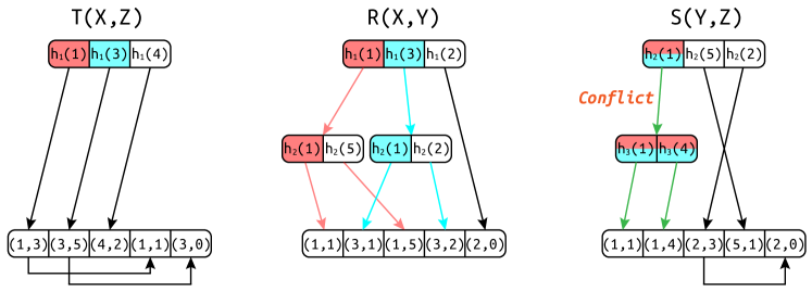
Figure 3. (Adapted from (Freitag et al., 2020b, Fig.6)) Conflicts in Traditional Parallel WCOJ Algorithm. The blue thread tries to access the sub-trie $h_{2}(1)$ in $S.Y$, while the red thread is constructing it.

Parallel GJ Logicblox(Aref et al., 2015) and Umbra (Freitag et al., 2020a) parallelilze GJ by partitioning the domain of the first variable $X_{1}$ into subsets of equal size, then computing the query on each subset in a separate thread, see Listing B in Fig. 1. The domains of $X_{2},X_{3},\ldots$ are not partitioned, and they will be scanned entirely by every thread, which leads to two important drawbacks. First, even if the domain of $X_{1}$ is uniformly distributed, the total work may be skewed: this can be seen for example in Fig. 2. Second, as shown in Fig. 3, since multiple threads access the same values of $X_{2},X_{3},\ldots$ they may attempt to construct concurrently the same fragment of the lazy trie, requiring the use of locks for synchronization (to avoid read/write conflicts), which introduces significant overhead. Those conflicting overheads are revealed by the scalability experiments of Umbra in Sec. 7.3.

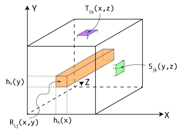
[HyperCube]HyperCube Partition

Figure 4. The HyperCube Partition

HyperCube Algorithm: The HyperCube algorithm (Afrati and Ullman, 2010; Beame et al., 2017; Koutris et al., 2016) computes the query (1) on a shared-nothing architecture with $P$ servers by partitioning all domains of all attributes. It organizes the $P$ servers into a hypercube with $n$ dimensions, by writing $P$ as a product $P=P_{1}\times P_{2}\times P_{n}$, such that each server is uniquely identified by $n$ coordinates, $(s_{1},\ldots,s_{n})$, with $s_{i}\in\{0,1,\ldots,P_{i}-1\}$. In the first step, HyperCube hash-partitions the domain of each variable $X_{i}$ into $P_{i}$ buckets then, in a single global communication step, it sends every tuple $R_{j}(\ldots)$ to all servers whose coordinates agree with the hash values of the tuple. In the second step, each of the $P$ servers computes the query on the fragment of relations it has received. The quantity $P_{i}$ is called the share of the variable $X_{i}$.

For example, consider the query $Q=R(X,Y),S(Y,Z),T(Z,X)$ and $P=4096$ severs. Hypercube writes $P=16\times 16\times 16$ and assigns to each server a unique combination of 3 coordinates $(s_{1},s_{2},s_{3})\in\{0,\ldots,15\}\times\{0,\ldots,15\}\times\{0,\ldots,15\}$, see Fig. 4. In the first step, it sends each tuple $R(x,y)$ to all of servers with the coordinates $(h_{X}(x),h_{Y}(y),*)$; each tuple $(y,z)$ in the relation $S$ is also sent to all servers $(*,h_{Y}(y),h_{Z}(z))$, and similarly for $T$. In the second step, each server computes the query on the relation fragments that it has received. Notice that each relation is replicated 16 times, for example each tuple $R(x,y)$ is sent to 16 servers, $(s_{1},s_{2},0),\ldots,(s_{1},s_{2},15)$.

A direct adaptation of HyperCube from the shared-nothing to a multicore, shared-memory architecture will have poor performance. The theoretical analysis in (Koutris and Suciu, 2016) addresses only the communication cost, i.e. the total number of tuples received by any server, and optimizes the shares $P_{1},P_{2},\ldots,P_{n}$ such as to minimize the communication cost. No algorithm is prescribed for the second step, and its computational cost is not analyzed. As we show in our paper, for multicores the choice of the variable order and the associated shares must be considered together.

Sparse Matrix Format:

The high-performance, and the sparse tensor compiler communities have developed as a suite of very efficient main memory representations for sparse tensors. Examples include Compressed Sparse Row (CSR), Compressed Sparse Column (CSC), Compressed Sparse Block (CSB) the Coordinate List (COO), Blocked Compressed Sparse Row (BCSR), Double Compressed Sparse Row (DCSR), see (Buluç et al., 2009), (Kjolstad et al., 2017, Fig.5) and (Chou et al., 2018, Fig.2). Our representation CoCo adapts ideas from sparse tensor representations for parallel evaluation of Generic Join.

Problem Statement The goal of this paper is to design efficient and scalable parallel variants of Generic Join; we will use the terms Generic Join and Worst Case Optimal Join interchangeably. As we saw, the traditional approaches to parallelization has several shortcomings. It is sensitive to data skew, causing some processors to be overloaded while others remain underutilized, thus degrading parallelization efficiency. The lazy trie construction read-write conflicts when executed in multi-threaded environments, which requires the use of locks for each index access. A third shortcoming (described in Sec. 6) is that some duplicated work that is inherent in Generic Join impacts the runtime, and this is more apparent in parallel implementations.

Our paper proposes, HoneyComb, designed to address these problems by ensuring better workload balance and avoiding conflicts during parallel execution. Additionally, HoneyComb is optimized for modern hardware architectures, by minimizing pointer chasing to improve memory access patterns and leveraging vector processing capabilities to accelerate operations.

3. Architecture of HoneyComb

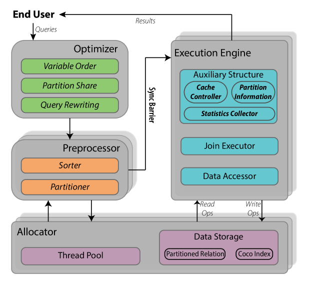
[Arch]The Architecture of HoneyComb

Figure 5. The Architecture of HoneyComb

HoneyComb takes as input a conjunctive query (see Eq. (1)) and evaluates it in parallel, using a fixed number of threads $P$; we use by default $P=1024$ threads. The threads are executed in parallel by all available cores on the system. Since HoneyComb assumes that the system has a large number of cores, e.g. dozens, it aims to avoid any synchronization between threads, because these can lead to significant slowdown when the number of cores is large.

HoneyComb uses the same partitioning method as HyperCube, by computing a number of shares $P_{i}$ for each query variable $X_{i}$, such that $P_{1}\times P_{2}\times P_{n}=P$, but, unlike HyperCube, it does not replicate the data, instead leverages the shared memory and allows threads to read concurrently. It optimizes both the variable order and the shares together. To avoid read-write conflicts, it precomputes all trie indices eagerly, using a novel index called CoCo, which is optimized for modern hardware architecture by minimizing pointer chasing and leveraging vector processing capabilities.

HoneyComb has four parts, see Fig. 5: the Optimizer, the Preprocessor, the Executor, and the Allocator.

The optimizer, described in Sec. 6, uses a cost model (Sec. 6.2) to determine both the variable order and the shares for each variable (Sec. 6.3). The optimizer also performs query rewriting to remove some redundant computations, described in Sec. 6.1.

Once the shares for each variable are computed, the Preprocessor (Sec. 4) sorts the input relations, physically partitions them, and builds the CoCo index for each partition. The partitioner is fully parallelized and its threads do not require coordination.

Finally, the Executor (Sec. 5) performs the actual work, by computing the query on each partition. The algorithm is similar to the standard Generic Join, with two exceptions: it uses our sort-based index CoCo instead of a hash-trie, and it may compute and store some intermediate results, as introduced by the optimizer during source rewriting. The executor is fully parallelized, and its threads do not require coordination; as we show in Sec. 7, this allows it to scale almost linearly up to 60 physical cores.

The Allocator uses use Intel Thread Building Block (TBB) to implement the scheduling framework (int, 2021). This is a standard task-stealing technique to execute threads on the available cores. The framework dynamically allocates computational tasks to cores, ensuring that all cores are engaged in meaningful work throughout the execution process. Moreover, the Allocator is designed to provide isolated partitioned data and cache for both the Executor and Preprocessor, minimizing contention and maximizing efficiency. Since this is a standard technique, we will not discuss the allocator in this paper any further.

4. The Preprocessor

The preprocessor is responsible for partitioning the input relations, and for computing the trie indices, called CoCo, for each partition. It receives the shares $P_{1},P_{2},\ldots,P_{n}$, and the variable order $X_{\sigma(1)},\ldots,X_{\sigma(n)}$ from the optimizer; for presentation purposes we assume in this and the next section that the variable order is $X_{1},X_{2},\ldots,X_{n}$, and we will revisit this in Sec. 6.

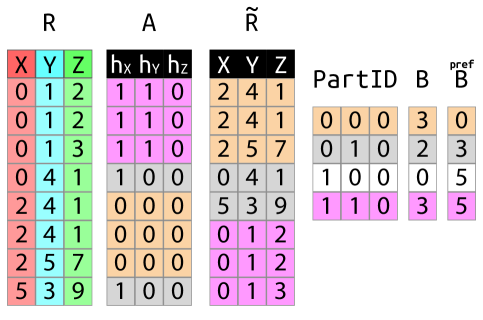
Figure 6. Parallel Partitioning

The input data is partitioned using the HyperCube method. The preprocessor chooses $n$ independent hash functions $h_{1},\ldots,h_{n}$, one for each query variable. We will assume w.l.o.g. that $h_{i}$ returns numbers in the set $\{0,1,\ldots,P_{i}-1\}$ (otherwise we replace it with $h_{i}(x)\mod P_{i}$). Initially, each input relation $R_{j}(X_{i_{1}},\ldots,X_{i_{k}})$ is stored in an array; we follow the C convention and assume array indices start at 0. Consider a $k$-tuple $(x_{1},\ldots,x_{k})$ of $R_{j}$. The quantities $s_{1}\stackrel{{\scriptstyle\text{def}}}{{=}}h_{i_{1}}(x_{1}),\ldots,s_{k}\stackrel{{\scriptstyle\text{def}}}{{=}}h_{i_{k}}(x_{k})$ are called the partition identifiers of this tuple. The preprocessor physically partitions $R_{j}$ into $\Pi_{j}\stackrel{{\scriptstyle\text{def}}}{{=}}P_{i_{1}}\!\times\cdots\times P_{i_{k}}\leq P$ chunks, called partitions, where each partition $R_{j,s_{1},\ldots,s_{k}}$ is a continuous array holding all tuples with partition identifiers $s_{1},\ldots,s_{k}$; all partitions are concatenated and stored in an output array $\tilde{R}_{j}$ of the same size as $R_{j}$. Unlike HyperCube, in HoneyComb there is no need to replicate $R_{j}$, instead, the partitioned data $\tilde{R}_{j}$ is an array of exactly the same size as $R_{j}$. As we discuss in the next section, during execution multiple threads will read from the same partition, taking advantage of the shared memory.

We describe now the details of the parallel partitioning step. First, HoneyComb computes (in parallel) the partition identifiers $(s_{1},\ldots,s_{k})$ of each tuple $(x_{1},\ldots,x_{k})$ in $R_{j}$, by applying the hash functions, and storing them in an array $A_{j}$, of the same size as $R_{j}$.

Next, it computes the size of each partition $R_{j,s_{1},\ldots,s_{k}}$ and stores them in a $k$-dimensional array $B_{j}$. Next, it computes a prefix sum on $B_{j}$ and stores the result in $B^{pref}_{j}$: notice that both $B_{j}$ and $B^{pref}_{j}$ have size $\Pi_{j}$ (the number of partitions of $R_{j}$), which is $\leq P$ (the total number of threads). $B_{j}$ is computed by scanning the tuples $(s_{1},\ldots,s_{k})$ in $A_{j}$ and incrementing $B_{j}[s_{1},\ldots,s_{k}]$; while $B^{pref}_{j}$ is the prefix sum of $B_{j}$, $B^{pref}_{j}[s_{1},\ldots,s_{k}]=\sum_{(t_{1},\ldots,t_{k})\preceq(s_{1},\ldots,s_{k})}B_{j}[t_{1},\ldots,t_{k}]$, where $\preceq$ represents lexicographic order. We did not parallelize the computations of $B_{j}$ and $B^{pref}_{j}$ because they turned out to represent only a tiny fraction of the total preprocessing time.

Finally, HoneyComb allocates the output array $\tilde{R}_{j}$ and copies the input tuples from $R_{j}$ into their respective partition $R_{j,s_{1},\ldots,s_{k}}$ in $\tilde{R}_{j}$: notice that this partition starts at position $B^{pref}_{j}[s_{1},\ldots,s_{k}]$ in $\tilde{R}_{j}$. Copying is done in parallel, using a number of threads equal to the number of available cores. Each thread is responsible for an exclusive subset of the $\Pi_{j}$ partitions: it scans the entire array $A_{j}$ and, if the current tuple $(s_{1},\ldots,s_{k})$ belongs to one of its partitions, then it physically copies the corresponding $R_{j}$-tuple to the partition $R_{j,s_{1},\ldots,s_{k}}$, otherwise it ignores the tuple.

There is no write contention between threads and the work is uniformly distributed. Since all threads need to read the entire vector $A_{j}$, in order to minimize the total amount of work, we restrict the number of threads to the number of physical cores. At the end of this phase, each partition $R_{j,s_{1},\ldots,s_{k}}$ is stored in a subarray of $\tilde{R}_{j}$, starting at the position $B^{pref}_{j}[s_{1},\ldots,s_{k}]$.

Example 4.1.

For a simple illustration, consider the Loomis-Whitney query, $Q=R_{1}(X,Y,Z),R_{2}(X,Y,U),$ $R_{3}(X,Z,U),R_{4}(Y,Z,U)$. Assume the variable order is $X,Y,Z,U$ and $P=2\times 2\times 1\times 2=8$.

In Fig. 6, we show a simple instance of the relation $R(X,Y,Z)$, the arrays $B,B^{pref}$ and the output $\tilde{R}$. For illustration, we made some arbitrary assumptions about the hash functions, e.g. $h_{Y}(1)=1$, $h_{Y}(4)=h_{Y}(5)=h_{Y}(3)=1$, shown in the relation $A$.

Each partition is color coded, and its tuples occur in a continuous subarray of $\tilde{R}$, e.g. the grey partition with identifiers $0,1,0$ consists of $(0,4,1),(5,3,9)$, has size $B[0,1,0]=2$ and starts at position $B^{pref}[0,1,0]=3$ in $\tilde{R}$. The white Partition $1,0,0$ is empty: $B[1,0,0]=0$.

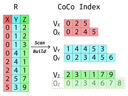
Figure 7. Construction of CoCo

Next, the preprocessor computes a trie index for each partition $R_{j,s_{1},\ldots,s_{k}}$ of each relation $R_{j}$. The index is a new and simple data structure that we call CoCo (Compressed Column layout), which combines ideas from both the trie in LFTJ (Veldhuizen, 2014) and the memory formats used by sparse tensor compilers (Chou et al., 2018). CoCo is defined as follows. For a $k$-ary relation $R(X_{1},\ldots,X_{k})$, CoCo consists of $k$ arrays $C_{1},...,C_{k}$. Each array $C_{r}$ contains the entire level $r$ of a sorted trie. Its entries are pairs $(x_{i},p_{i})$, where $x_{i}$ is a value of $R.X_{i}$ and $p_{i}$ is an index to the beginning of a subarray of $C_{i+1}$. The top vector consists of all distinct values $x_{1}$ in $R.X_{1}$, sorted in ascending order, and, for each pair $(x_{1},p_{1})$ in $C_{1}$, the index $p_{1}$ represents the beginning of a subarray in $C_{2}$ that contains all distinct values $x_{2}$ in $R[x_{1}].X_{2}$. And so on. The last vector $C_{k}$ has pointers in the data array $R$. HoneyComb constructs a separate CoCo index for each partition, $R_{j,s_{1},...,s_{k}}$ of the relation $R_{j}$.

To build CoCo, we sort the partitions $R_{j,s_{1},\ldots,s_{k}}$ lexicographically, according to the variable order provided by the optimizer: recall that we assumed, for simplicity, that the order is $X_{1},\ldots,X_{K}$. For example for the triangle query in Fig. 1, if the order is $X,Y,Z$ then the relation $T(Z,X)$ will be sorted by $X$ first then by $Z$. Since each partition $R_{j,s_{1},\ldots,s_{k}}$ is a subarrays of a larger array $\tilde{R}_{j}$, there are two possibilities to sort it. One is to sort each partition independently, in parallel threads; we do this when the number of partitions $\Pi_{j}$ of $R_{j}$ is larger than the number of available cores. If $\Pi_{j}$ is too small (e.g. when all shares $P_{i}$ of all variables in $R_{j}$ are $=1$), then we use a single parallel sorting function and sort together the pair of arrays $A_{j},\tilde{R}_{j}$, thus forcing the tuples with the same partition to stay together. For this purpose we use ips4o (In-place Parallel Super Scalar Samplesort) (Axtmann et al., 2017, 2020), which is a highly optimized parallel sorting function for multicores.

Next, for each sorted partition $R_{j,s_{1},...,s_{k}}$, the CoCo is constructed by compressing the same column values with the same prefix determined by the variable order. For each variable $X_{r}$, the array $C_{r}$ consists of two separate arrays $V_{r},O_{r}$, where $V_{r}$ for the values of $X_{r}$ and $O_{r}$ for offsets into $C_{r+1}$.

We first scan over all rows in the partition by computing the number $l_{r}$ of unique values with prefix $(\ldots,s_{r})$ for any attribute $X_{r}$. Then, we allocate the space with $l_{r}$ size for $V_{r}$ and $l_{r}+1$ size for $O_{r}$ and scan again to populate them from bottom to above. During the second pass, we bookkeep a cursor about current offset $o_{i}$ in the compressed array for each attribute and sequentially compare the adjacent two rows $(s_{1},\ldots,s_{k})$ and $(t_{1},\ldots,t_{k})$ and find the index $e$ of the first differing element $s_{e}\neq t_{e}$ but $(s_{1},\ldots,s_{e-1})=(t_{1},\ldots,t_{e-1})$. Then, we create a new entry in $V_{e}$ with the value $t_{e}$ and the offset $o_{e}$ in $O_{e}$, and increment $o_{e}$. Moreover, since the prefix is changed, we need to create entries with value $t_{d}$ and offset $o_{d}$ for any $V_{d},O_{d}$ with any $d>e$ and increment $o_{d}$ as well. Besides, if the relation is unique, we will ignore the offset vector of last attribute $O_{k}$ and its construction.

Example 4.2.

In Fig. 7, we show the CoCo index for the relation $R(X,Y,Z)$. The first vector $C_{1}=C_{X}$ contains all distinct values $V_{X}$ of $X$ and the offsets $O_{X}$ in the $C_{Y}$ (starts with $0$). The second vector $C_{2}=C_{Y}$ depends on the prefix of $X$ and contains all values $V_{Y}$ of $Y$ with different $X$, thus we can see two $4$ in the $V_{Y}$ since they have different $X$ values. The last vector $V_{3}=V_{Z}$ is just similar cases, but the last level offsets $O_{3}=O_{Z}$ will be removed if the relation $R$ itself is distinct.

5. Executor

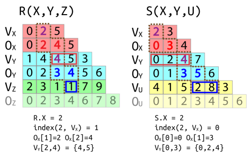
Figure 8. Join Execution on CoCo

After preprocessing, the Executor computes Generic Join, in parallel. Recall that the query $Q$ in Eq. (1) has $n$ variables $X_{1},\ldots,X_{n}$. The optimizer has computed the shares $P_{1},\ldots,P_{n}$ for each variable, and has chosen a variable order, which we assume w.l.o.g. is $X_{1},\ldots,X_{n}$, while the preprocessor has partitioned each input relation $R_{j}$ and moved it to a new array $\tilde{R}_{j}$.

The executor assigns each partition to a thread with identifier $(s_{1},s_{2},\ldots,s_{n})$. Each thread executes Generic Join independently, with the only difference that, for each relation $R_{j}(X_{i_{1}},\ldots,X_{i_{k}})$, it only accesses the subarray of $\tilde{R}_{j}$ corresponding to the partition $R_{j,s_{i_{1}},\ldots,s_{i_{k}}}$, which starts at offset $C_{j}[s_{i_{1}},\ldots,s_{i_{k}}]$ in $\tilde{R}_{j}$. Otherwise, the structure of the executor is the same as that of the standard generic join: a sequence of nested loops, each corresponding to a variable $X_{i}$. The main work is done by the intersection $R_{j_{1}}.X_{i}\cap R_{j_{2}}.X_{i}\cap\cdots$, which we describe in detail next. Notice that the total number of threads is the total number of output partitions, which is $P_{1}\times P_{2}\times\cdots\times P_{n}=P$. Also, there is no read-write conflict between threads: their only interaction is that they read from the shared memory. Besides, due to non-overlapping join results, each thread can store its outputs in its local memory; at the end of the computation, these results can be concatenated if needed.

Listing C in Fig. 1 shows the execution performed by the thread with the identifier $(i,j,k)$; this thread only needs to access the partitions $R_{ij},S_{jk}$, and $T_{ik}$, and join them.

Next, we present the details of the intersection, which is the main work done in WCOJ. By using CoCo, the intersection needs to compute common values in a set of sorted and contiguous arrays. For this purpose, HoneyComb uses ideas from multi-way merge.

Given a sorted array $V$ and a value $x$, the method $\text{search}(V,x)$ (described below) that finds the position of the first element in $V$ that is $\geq x$. To compute the intersection of multiple arrays $V_{1}\cap V_{2}\cap\cdots$ we use a cursor in each array, and maintain the minimum min and maximum max values among all cursors. If $\text{max}\neq\text{min}$, we just advance the cursor of min to $\text{search}(V_{j},\text{max})$; otherwise, we have found a common value $\text{min}=\text{max}$.

For the first attribute $X_{1}$ in variable order, the intersection $R_{j_{1}}.X_{1}\cap R_{j_{2}}.X_{1}\cap\cdots$ is done by the above procedure on the first levels $V_{1}$ in CoCo of $R_{j_{1}},R_{j_{2}},\ldots$. Once we encounter a value $X_{1}=x$ present in all relation, for each relation $R_{j_{k}}$ we need to restrict the range of next trie level. Assuming that $x$ occurs on position $\mathrm{index}$ in $V_{1}$, then the next level will be restricted to the subarray $V_{2}[O_{1}[\mathrm{index}]:O_{1}[\mathrm{index}+1]-1]$. In general, each intersection will be done by intersecting several arrays, which can be either a full CoCo array $V_{r}$, or a subarray thereof.

Example 5.1.

In Fig. 8, The area surrounded by the brown line shows a state during the join between $R(X,Y,Z)$ and $S(X,Y,U)$ on the CoCo. Now, we already find that $R.X=S.X=2$ is an intersection on the attribute $X$. To find the intersecting range of $Y$ in $R$, we need compute the $\mathrm{index}(R.X,V_{X})=1$, and obtain the range $[O_{X}[1],O_{X}[2])=[2,4)$ in the $V_{Y}$, which is the subarray $\{4,5\}$. The similar case happened on $S.Y$ and obtained the subarray $\{0,2,4\}$. Then we do the intersection on two subarrays and find the intersected value $Y=4$.

To further improve the intersections on sorted arrays efficiently, we propose three $search$ ways, which are Exponential, Quadratic, and Linear, and use them based on the number of attributes involved in the intersection. Exponential Search (Baeza-Yates and Salinger, 2010), also known as galloping search, is suitable when dealing with skewed and large datasets. It begins by jumping exponentially (i.e., $2^{n}$) through the data until it overshoots the target value, after which it switches to a binary search within the identified range. Quadratic Search is somehow used for medium-sized datasets and involves first a series of steps that increase by fixed size which is set to the multiple of cache line size, and then scan within identified range or recursively apply Quadratic search (but unrolling in implementation). Finally, Linear Search is employed for small datasets, as it is the most efficient search method for a small number of elements which is fitted the cache size. By selecting the appropriate search method based on the size of the intersection, we ensure that the join operation is optimized for each scenario, maximizing efficiency and performance.

6. Optimization

The optimizer in HoneyComb has three goals: it chooses shares $P_{1},\ldots,P_{n}$ for the variables $X_{1},\ldots,X_{n}$, it chooses a variable order $X_{\sigma(1)},\ldots,X_{\sigma(n)}$ to be used by the query executor, and, finally, it performs a rewriting of the code of Generic Join in order to remove redundant computations inherent in this algorithm. All decisions are done jointly, and are informed by a cost model described in Sec. 6.2. Although it happens last, we start our presentation of the optimizer by describing query rewriting.

6.1. Query Rewriting

Recall that Generic Join consists of $n$ nested loops, one loop for each variable $X_{i}$. The actual work in GJ consists of computing the intersection of all columns of the variables $X_{i}$. For complex queries, some of these intersections computed in the inner loops are independent of outer loop and, thus, are repeated unnecessarily for each iteration of the outer loop. In this case our optimizer rewrites the query such as to compute the intersection early, and stores this as a temporary result. We illustrate query rewriting with an example; the general case follows immediately.

⬇

Q(X,Y,Z,U) = R1(X,Y), R2(X,Z), R3(X,U),

 R4(Y,Z), R5(Y,U), R6(Z,U).

// BEFORE REWRITING

For x $\in$ R1.X $\cap$ R2.X $\cap$ R3.X

For y $\in$ R1[x].Y $\cap$ R4.Y $\cap$ R5.Y

For z $\in$ R2[x].Z $\cap$ R4[y].Z $\cap$ R6.Z

For u $\in$ R3[x].U $\cap$ R5[y].U $\cap$ R6[z].U

Q += (x, y, z, u)

⬇

// AFTER REWRITING

tmp_Y := R4.Y $\cap$ R5.Y // Lift Up Y

For x $\in$ R1.X $\cap$ R2.X $\cap$ R3.X

tmp_Z := R2[x].Z $\cap$ R6.Z // Lift Up Z

For y $\in$ R1[x].Y $\cap$ tmp_Y

tmp_U := R3[x].U $\cap$ R5[y].U // Lift Up U

For z $\in$ R4[y].Z $\cap$ tmp_Z

For u $\in$ R6[z].U $\cap$ tmp_U

Q += (x, y, z, u)

Figure 9. Example of Query Rewriting

Example 6.1 (Duplicated Intersections).

Consider the following query which computes a 4-clique $Q$ on the variables $(X,Y,Z,U)$. Generic Join for $Q$ is shown in Fig 9 (left), with three pieces of redundant work highlighted. They do not depend on the current loop variable, and therefore are computed repeatedly:

Here $R4[y].Z$ represents the column $Z$ of the subset of $R4$ where $Y=y$.

For example, R4.Y $\cap$ R5.Y is computed repeatedly, for every value $x$, although this expression does not depend on $x$.

Given the variable order, our optimizer identifies intersections that can be cached, then

proceeds to ”lift” these intersections, treating them as independent computational entities. These independent intersections are then computed only once before the iteration over the current loop variable and cached within auxiliary data structures. This process not only reduces the need for repeated calculations but also ensures that these pre-computed intersections can be efficiently accessed and reused across different parts of the join operation.

Example 6.2.

The optimizer rewrites the code above as follows:

Instead of computing the intersection $R1[x].Y\cap R4.Y\cap R5.Y$ for each $x$, we compute $R4.Y\cap R5.Y$ before starting the iteration on $x$ and cache the result in a temporary sorted array tmp_Y, as shown in Fig 9 (right). Then, during the iteration over $x$, we intersect $R1[x].Y$ with tmp_Y. Importantly, the temporary array tmp_Y also stores offsets corresponding to the value $y$ in the CoCo of $R4$ and $R5$.

While this optimization does not improve the asymptotic runtime of WCOJ, it can improve the actual runtime. To see this, consider how WCOJ computes the intersection $R1[x].Y\cap R4.Y\cap R5.Y$. Denoting the three sorted arrays $R1[x].Y$, $R4.Y$, $R5.Y$ by $A,B,C$ respectively, the simplified pseudocode is shown in Fig. 10: notice that HoneyComb uses exponential search instead of the linear search, see Sec. 5. By precomputing the intersection of $B\cap C$, we replace a 3-way merge with two 2-way joins, which avoids repeating the same iterations over $B,C$ for every value of $x$, and also have a simpler code and better cache locality.

⬇

i = j = k = 0;

while not done:

if A[i] = B[j] = C[k]:

output(A[i]);

i++, j++, k++;

while (A[i] < min(B[j], C[k])):

i++;

while (B[j] < min(A[i], C[k])):

j++;

while (C[k] < min(A[i], B[j])):

k++;

⬇

j = k = p = 0;

while not done:

if B[j] = C[k]:

Tmp[p++] = B[j++]; j++, k++;

while (B[j] < C[k]): j++;

while (C[k] < B[j]): k++;

. . . .

i = p = 0

while not done:

if A[i] = Tmp[p]:

output(A[i]); i++, p++;

while (A[i] < Tmp[p]): i++;

while (Tmp[[p] < Ai]): p++;

Figure 10. Simplified Pseudocode for computing $A\cap B\cap C$, and same code that caches $B\cap C$ before computing the intersection. HoneyComb uses exponential search (Sec. 5) instead of the linear search shown here. Notice that these two code fragments are equivalent only if $A,B,C$ are sorted arrays.

We note that this query rewriting is a logical optimization, and is not an optimization that can be done by a compiler, e.g. by using LLVM Loop Invariant Code Motion (-licm) pass. A simple reason is that there is no piece of code in Fig. 10 (left) that represents $B\cap C$, which the compiler could attempt to move. A deeper reason is that the optimization in Fig. 10 is sound only if the arrays $A,B,C$ are sorted, which is an invariant that compilers usually cannot infer.

HoneyComb stores each temporary intersection locally in each thread. There are no read-write or write-write conflicts between threads during the parallel execution. Each thread only operates on its locally cached data, and there is no need for a lock-based synchronization. Therefore this optimization reduces duplicated work, without creating additional bottlenecks.

Next, we discuss the complexity of the optimized algorithm. A fractional edge cover of the full conjunctive query in Eq. (1) is a tuple of non-negative numbers $\bm{w}=(w_{1},\ldots,w_{m})$ such that “every variable $X$ is covered”, meaning $\sum_{j:X\in\text{Vars}(R_{j})}w_{j}\geq 1$. It is known that, for any fractional edge cover $\bm{w}$, Generic Join runs in time $\tilde{O}(\prod_{j}|R_{j}|^{w_{j}})$. Consider now an optimized algorithm $P$, where some intersections have been cached early, and let $Q_{P}$ the query obtained from $Q$ as follows: $Q_{P}$ has the same atoms $R_{j}$ as $Q$, and each variable $X$ occurs only in those atoms $R_{j}$ that are used in the first intersection of the $X$ domains. We prove in the full version of the paper:

Theorem 6.3.

For any fractional edge cover $\bm{w}$ of $Q_{P}$, algorithm $P$ runs in time $\tilde{O}(\prod_{j}|R_{j}|^{w_{j}})$.

To illustrate, consider the query $Q$ in Example 6.1. If $R_{2},R_{5}$ are the smallest of the 6 relations, then standard Generic Join runs in time $\tilde{O}(|R_{2}|\cdot|R_{5}|)$, because of the fractional edge cover $\bm{w}=(0,1,0,0,1,0)$. The query $Q_{p}$ associated to the program $P$ in Example 6.2 is $Q_{P}=R_{1}(X)\wedge R_{2}(X,Z)\wedge R_{3}(X,U)\wedge R_{4}(Y)\wedge R_{5}(Y,U)\wedge R_{6}(Z)$ ($Y$ only occurs in $R_{4},R_{5}$ because of $\text{tmp}_{Y}:=R_{4}.Y\cap R_{5}.Y$). Since $\bm{w}$ is also a fractional edge cover of $Q_{P}$, algorithm $P$ runs in optimal time $\tilde{O}(|R_{2}|\cdot|R_{5}|)$; in particular, $P$ is optimal when $|R_{1}|=\cdots=|R_{6}|=N$. However, if $R_{1},R_{6}$ are strictly smaller than all other relations, then $P$ is no longer optimal.

If theoretical optimality is required, it is possible to check for each candidate rewriting $P$ if its complexity is the same as that of standard generic join. In HoneyComb we use a cost model instead, as we describe next.

6.2. Cost Model

We describe here our model for estimating the cost of Generic Join on the query $Q$ in (1), assuming a variable order $\bm{X}_{\sigma}$ given by a candidate permutation $\sigma$, i.e. $X_{\sigma(1)},X_{\sigma(2)},\ldots,X_{\sigma(n)}$; refer to the notations in Table 1.

Consider some level $i=1,n$. The outer iterations have bound their variables to the prefix $x_{\sigma(1:i-1)}\stackrel{{\scriptstyle\text{def}}}{{=}}(x_{\sigma(1)},x_{\sigma(2)},\ldots,x_{\sigma(i-1)})$. Let $\mathcal{S}[X_{\sigma(i)}]=\{R_{j_{1}},R_{j_{2}},\ldots\}$ (or just $\mathcal{S}$ when the variable $X_{\sigma(i)}$ is clear from the context) be the set of relation names that contain the variable $X_{\sigma(i)}$, and $|\mathcal{S}|$ be its size. Then the $i$’th loop needs to compute $R_{j_{1}}[x_{\sigma(1:i-1)}].X_{\sigma(i)}\cap R_{j_{2}}[x_{\sigma(1:i-1)}].X_{\sigma(i)}\cap\cdots$. We denote by $\mathcal{N}[x_{\sigma(1:i-1)}\oplus X_{\sigma(i)}]$ the set of cardinalities of the relations in $\mathcal{S}$, i.e. $\{|R_{j_{1}}[x_{\sigma(1:i-1)}]|,|R_{j_{2}}[x_{\sigma(1:i-1)}]|,\ldots\}$, and by $\min\mathcal{N}$, $\max\mathcal{N}$ the smallest/largest cardinality. For example, consider the triangle query in Fig. 1, where the variable order is $X,Y,Z$. In the second loop ($\texttt{for }y\texttt{ in}\ldots$), we have $\mathcal{S}=\mathcal{S}[x\oplus Y]=\{R[x],S\}$, $|\mathcal{S}|=2$, and $\mathcal{N}[x\oplus Y]$ is $\{|R[x]|,|S|\}$. If $|R[x]|<|S|$, then $\min\mathcal{N}=|R[x]|$ and $\max\mathcal{N}=|S|$.

Next, we describe the cost of computing the intersection at level $i$, which we denote by ${\mathcal{C}}[{{\bm{x}_{\sigma({1:i-1})}}\oplus{\bm{X}_{\sigma({i})}}}]$. Assume that the intersection is computed using galloping search: iterate over the smallest relation $R_{j_{\min}}$ with the cardinality $\min\mathcal{N}[x_{\sigma(1:i-1)}\oplus X_{\sigma(i)}]$, and probe using exponential search in each of the remaining relations $R_{j}$. If the values in $R_{j_{\min}}$ are uniformly distributed in $R_{j}$, then the cost is $\log\frac{|R_{j}|}{|R_{j_{\min}}|}$, which leads to:

$${\mathcal{C}}[{{\bm{x}_{\sigma({1:i-1})}}\oplus{\bm{X}_{\sigma({i})}}}]=|{\mathcal{S}}[{{\bm{X}_{\sigma({i})}}}]|\cdot\min{\mathcal{N}}[{{\bm{x}_{\sigma({1:i-1})}}\oplus{\bm{X}_{\sigma({i})}}}]\cdot\log_{2}\Big{(}1+\frac{\max{\mathcal{N}}[{{\bm{x}_{\sigma({1:i-1})}}\oplus{\bm{X}_{\sigma({i})}}}]}{\min{\mathcal{N}}[{{\bm{x}_{\sigma({1:i-1})}}\oplus{\bm{X}_{\sigma({i})}}}]}\Big{)}$$

So far the cost is for a single binding $\bm{x}_{\sigma(1:i-1)}$ of the prefix $\bm{X}_{\sigma(1:i-1)}$ of the variables. To add up their cost, we need a notation. Consider our definition of the conjunctive query in Eq. (1): the head variables are $X_{1},\ldots,X_{n}$. We denote by $Q(\bm{X}_{\sigma(1:i-1)})$ the query where the head variables are restricted to $\bm{X}_{\sigma(1:i-1)}$. The bindings $\bm{x}_{\sigma(1:i-1)}$ will iterate over all outputs of this query, hence the total cost at the level $i$ is:

$${\mathcal{C}}[{{\bm{X}_{\sigma({1:i})}}}]=\qquad\smashoperator[lr]{\sum_{{\bm{x}_{\sigma({1:i-1})}}\in Q(\bm{X}_{\sigma(1:i-1)})}^{}}\qquad{\mathcal{C}}[{{\bm{x}_{\sigma({1:i-1})}}\oplus{\bm{X}_{\sigma({i})}}}]$$

Ultimately, we define the total cost $\mathbb{C}[\bm{X}_{\sigma}]$ of our join algorithm by summing up the intersection costs for all variables in the variable order $\bm{X}_{\sigma}$.

$$\mathbb{C}[\bm{X}_{\sigma}]=\mathbb{C}[{\bm{X}_{\sigma({1:n})}}]=\smashoperator[lr]{\sum_{i\in[n]}^{}}{\mathcal{C}}[{{\bm{X}_{\sigma({1:i})}}}]$$

This cost cannot be computed exactly at optimization time, instead we compute an upper bound. For that purpose we use a pessimistic cardinality estimator (Cai et al., 2019; Khamis et al., 2024; Abo Khamis et al., 2024) to upper bound the output size of the queries $Q(\bm{X}_{\sigma(1:i-1)})$, and use the following inequality, which we prove in the full version of the paper:

Lemma 6.4.

The following inequality holds, where the summation is over $\bm{x}_{\sigma(1:i-1)}\in Q(\bm{X}_{\sigma(1:i-1)})$, and we drop the argument ${\cdot}[{{\bm{x}_{\sigma({1:i-1})}}\oplus{\bm{X}_{\sigma({i})}}}]$ from $\mathcal{N}$:

(2) $${\mathcal{C}}[{{\bm{X}_{\sigma({1:i})}}}]\leq|\mathcal{S}(X_{\sigma(i)}|\cdot(\sum\min\mathcal{N})\cdot\log_{2}\Big{(}1+\frac{\sum\max\mathcal{N}}{\sum\min\mathcal{N}}\Big{)}$$

Example 6.5.

Referring again to the 2nd loop of the triangle query, $R[x].Y\cap S.Y$, we have $\mathcal{N}=\{|R[x]|,|S|\}$. We compute Eq. (2) as follows. First, $\sum\min\mathcal{N}$ is $\sum_{x}\min(|R[x].Y|,|S.Y|)$, which is the same as the output size of the query $Q(X,Y)=R(X,Y),S(Y),T(X)$ (where $S(Y),T(X)$ represent $\Pi_{Y}(S)$ and $\Pi_{X}(T)$ respectively). We upper bound it using a pessimistic cardinality estimator: HoneyComb uses (Abo Khamis et al., 2024) for this purpose. For the expression inside the logarithm $\dfrac{\sum_{x}\max(|R[x].Y|,|S.Y|)}{\sum_{x}\min(|R[x].Y|,|S.Y|)}=\dfrac{\mathop{avg}_{x}\max(|R[x].Y|,|S.Y|)}{\mathop{avg}_{x}\min(|R[x].Y|,|S.Y|)}$. Since this does not have a closed form, we estimate it as $\dfrac{\max(\mathop{avg}_{x}(|R[x].Y|),\mathop{avg}_{x}(|S.Y|))}{\min(\mathop{avg}_{x}(|R[x].Y|),\mathop{avg}_{x}(|S.Y|))}$. Next, we compute $\mathop{avg}_{x}(|R[x].Y|)=|R|/|R.X|$, and similarly for the other terms. The 1st and the 3rd loops of the triangle query are handled similarly.

If an intersection at level $i$ is rewritten to be computed at an earlier level $i_{0}<i$ (Sec. 6.1), then those relations will be included in the set $\mathcal{S}(X_{\sigma(i_{0})})$, while the temporary relation will be added to $\mathcal{S}(X_{\sigma(i)})$.

6.3. Plan Decision

We describe now how the optimizer chooses the optimal variable order, $\bm{X}_{\sigma}$ and shares $P_{1}\times P_{2}\times\cdots\times P_{n}=P$, where $P_{i}$ represents the share of the variable $X_{\sigma(i)}$.

The HyperCube partition leads implicitly to some replicated work, which we capture by the following expressions:

(3) $${\mathbb{C}}[{\bm{X}_{\sigma},\bm{P}_{\sigma}}]=\smashoperator[lr]{\sum_{i\in[n]}^{}}\Big{(}(\prod_{j>i}P_{\sigma(j)}){\mathcal{C}}[{{\bm{X}_{\sigma({1:i})}}}]\Big{)}$$

For example, in the triangle query, for a fixed $x$, every value $y\in R[x].Y\cap S.Y$ is discovered redundantly by all threads with partition identifiers the form $(i,j,*)$ where $i=h_{X}(x)$ and $j=h_{Y}(y)$: this accounts for the product $\prod_{j>i}$ above.

A naive way to compute the optimal variable order $\sigma$ and shares $P_{i}$ is to try all combinations and return the cheapest cost (3). There are $n!$ variable orders and ${10+n-1\choose n-1}$ total possible share allocations (since we use by default $P=1024=2^{10}$ threads). A brute force search only works for small values of $n$. Instead, we apply some pruning heuristics, as follows.

We prune partition shares that increase the cost ${\mathbb{C}}[{\bm{X}_{\sigma},\bm{P}_{\sigma}}]>2\cdot{\mathbb{C}}[{\bm{X}_{\sigma}}]$. We will also prune small partitions. Recall that if we throw randomly $B$ balls into $P$ bins and $B=O(N)$, then the expected size of the largest bin is not $O(B/P)=O(1)$, but it is $O(\log P)$, which means that the data is non-uniformly distributed. To expect uniform distribution, $O(B/P)$, we need $B>3P\log P$ balls (Koutris and Suciu, 2016). Therefore, we prune partitions containing some share $P_{i}$ where $|\textsf{Dom}(X_{i})|<3\cdot P_{i}\cdot\log P_{i}$

Finally, we assign an eveness score $E$ to a set of shares, which favors evenly distributed, with a bias towards have more shares for last variables $X_{\sigma(n)},X_{\sigma(n-1)},\ldots$ than for the first variables. $E$ is defined as:

(4) $$E(\bm{P}_{\sigma})=\sum_{i\in[n]}P_{\sigma(i)}\cdot w(i)$$

where $w(i)=\max\{1-\frac{i}{100},\frac{3}{4}\}$ is a smooth weight function on $i$ to distinguish the importance of the variable. Finally, we choose the partition share with the minimum evenness among all feasible partitions, to balance the task computations and avoid data skewness.

7. Experiments

We implemented HoneyComb as a standalone C++ program. It reads the query and the data path from a JSON file, and loads data from a binary file, which was previously converted from CSV format. After running the query, the program can either output all result tuples, or output only the count. We compared HoneyComb against some state-of-the-art systems that support cyclic join queries, and conducted some scalability and ablation studies. We ask four research questions:

1. How does the absolute performance of HoneyComb compare to that of related systems on both real and synthetic datasets?

2. How does HoneyComb scale up with an progressively increased number of cores?

3. How important is it to optimize the partition shares and the variable order?

4. How effective is the query rewriting method and the CoCo data structure?

7.1. Setup

Table 2. Dataset Characteristics

Name	# Node	# Edge	Feature
WGPB (wgp, 2019; Hogan et al., 2019)	54.0M	81.4M	sparse, skew
Orkut (Mislove et al., 2007)	$3.07M$	$117M$	partial dense, uniform
GPlus (McAuley and Leskovec, 2012)	107K	13.6M	dense, skew
USPatent (Leskovec et al., 2005)	3.77M	16.5M	sparse, uniform
Skitter (Leskovec et al., 2005)	1.69M	11.1M	sparse, partial skew
Topcats (Yin et al., 2017)	1.79M	28.5M	partial dense, skew

Datasets: We provide the information for our graph datasets in Table 2. These datasets include a variety of types, sparsity, and skewness, which cover the common characteristics of real-world datasets.

We transform those datasets into CSV format and either load them directly or use the provided loader to fetch them to the main memory.

In addition, we also use two synthetic datasets for tensor kernels, with different sparsity. We generate the synthetic datasets with the same number of nodes and hyperedges where the number of attributes is set to 3. The first dataset (named ST-Dense) is generated uniformly densely distributed. The dataset consists of 7 relations, each with three attributes. The first four relations follow the form $[512]\times[512]\times[512]$. The last three relations have attribute domains $(\{0,1\}|\{0,2\}|\{1,2\})\times[4096]\times[4096]$. The second dataset (named ST-Sparse) is similar but just distributed sparsely. The first four relation randonly selected $512^{3}$ tuples from $[5120]\times[5120]\times[5120]$, the sparsity is $0.001$. The last three relations are selected $4096^{2}$ tuples from $[40960]\times[40960]$ while keeping the first attribute, thus the sparsity is $0.01$.

Baselines: We compare our method with five state-of-the-art baselines: Umbra (Freitag et al., 2020a), Diamond (Birler et al., 2024), DuckDb (Raasveldt and Mühleisen, 2020), Soufflé (Arch et al., 2022), and Kùzu (Jin et al., 2023).

Umbra (2022-11-03) is a high-performance database management system designed for modern hardware architectures. It nicely supports the worst-case optimal join (multiway join) algorithms in parallel through morsel-driven execution. Diamond is a variant of Umbra, which is optimized to solve the diamond problem. It splits join operators into Lookup and Expand suboperators, and allows them to be freely reordered. It also uses a novel ternary operator Expand3 that implements the triangle query. Kùzu (v0.6.0) is a graph database engine that excels at handling complex queries involving joins across graph-structured data. Its most recent version it supports worst-case optimal join through “join hints” (kuz, 2024). Soufflé (v2.4.1) is a logic-based database engine that compiles queries into optimized C++ code. It supports efficient execution of Datalog queries, particularly for complex join operations, but does not implement worst-case optimal join. DuckDB (v1.1.1) is an in-process analytical database management system optimized for fast OLAP workloads. It is heavily optimized for complex join queries, but does not support worst-case optimal join.

Umbra is provided in binary format and was obtained directly from the author, while the other baselines are open-source and were downloaded directly from their official GitHub repositories.

For Umbra, we enabled paged storage optimization, and forced it to use worst-case optimal join, which improved its performance. For Soufflé, we enabled brie representation for dense input relation, which also improved its performance. For Kùzu, we provided join order hints in order to facilitate the worst-case optimal join plan. All these non-default settings were chosen to improve the systems’ overall performance.

Table 3. Table of Queries

Name	Queries
Q1 (Triangle)	Q(X,Y,Z) := R(X,Y), S(Y,Z), T(X,Z).
Q2 (4-Loop)	Q(X,Y,Z,U) := R1(X,Y), R2(X,Z), R3(Y,U), R4(Z,U).
Q4 (4-Diamond)	Q(X,Y,Z,U) := R1(X,Y), R2(X,Z), R3(Y,U), R4(Z,U), R5(Y,Z).
Q6 (4-Clique)	Q(X,Y,Z,U) := R1(X,Y), R2(X,Z), R3(Y,U), R4(Z,U), R5(Y,Z), R6(X,U).
Q8 (2-Triangle)	Q(X,Y,Z,U,V) := R1(X,Y), R2(X,Z), R3(Y,Z), R4(Z,U), R5(Z,V), R6(U,V).
LW(Loomis-Whitney) ​​​	Q(X,Y,Z,U) := R1(X,Y,Z), R2(X,Y,U), R3(X,Z,U), R4(Y,Z,U).
CT (Clover-Triangle)	Q(U,X,Y,Z) := R5(U,X,Y), R6(U,X,Z), R7(U,Y,Z).

Queries: We evaluate the performance of our method and baselines on the queries listed in Table 3. The first five query patterns are derived from the paper (Mhedhbi and Salihoglu, 2019), and are used for graph datasets, while the latter are typical sparse tensor kernels (Kjolstad et al., 2017). For the triangle query, Q1, we used two variations, Q1d and Q1u, representing triangles on a directed and undirected graph respectively. We run all other queries only on the directed graphs.

Metrics: We evaluate the performance of HoneyComb and other systems by measuring their overall execution time. Specifically, we track the wall-clock time taken by each system to complete each query from start to finish. This timing excludes the duration spent on data loading, result output, and data statistics collection, but it does account for the time used to create indexes.

We conduct each measurement three times and report the average runtime. For Soufflé, we also exclude the compilation time and report only the runtime of the generated programs after compilation. For Umbra and Kùzu, we run the query one extra time initially, to avoid the cold start issue, such as additional query compilation or data loading time. We set a timeout of 10,000 seconds for each individual experiment repetition. Any timeout is marked by X in our graphs.

Environment: We conduct our experiments on Intel Xeon Phi Server, which has 60 cores and 120 hyperthreads on 4 sockets, as well as 1TB main memory. Except Umbra, HoneyComb and the open-source baselines are all compiled using GCC 13.3.0 with Release mode on Rocky Linux 9.4.

7.2. Performance Comparison

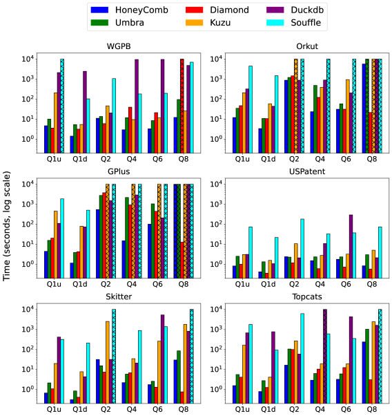
Figure 11. Performance Comparison on Graph Datasets. An X means “timeout after 10,000 seconds”

Our first set of experiments compares the runtime of HoneyComb and the other baselines on graph datasets, using all the 60 available cores. The results, in Fig. 11, show that HoneyComb consistently outperforms the other systems across all queries and datasets, with significant runtime reductions observed in most cases, with the exception of Diamond, which it outperforms on most but not all queries (more on this below).

On dense datasets, such as GPlus and Orkut, HoneyComb benefits from rewriting and CoCo while it efficiently supports lookup and scan over the sorted dense data. Umbra incurs an overhead during the construction of the hash trie since most of the sub-tries are touched and need to be built. Kùzu, despite using hints for generic join order, is slower than Umbra. DuckDB, although it does not support the worst-case optimal join and generally lags behind the others, it performed quite well on the 4-loop query Q2, because Q2 has a small tree-width (Khamis et al., 2016), where the advantage of the worst-case optimal join over traditional plans diminishes. Soufflé is the slowest, where almost all queries are timeout, mainly due to the lack of optimizations for both binary and generic joins.

For sparse datasets, such as WGPB, HoneyComb continues to outperform the other systems, but the gap between HoneyComb and Umbra narrows. Based on the description of (Freitag et al., 2020a) we believe that Umbra’s lazy trie construction is more effective for sparse data than for dense data, because there are fewer contentions between threads and fewer sub-trie structures to be constructed on demand. On sparse data, HoneyComb benefits from the partitioning strategy, which helps reduce the computational skew. In contrast, both Umbra and Kùzu partition only on the first attribute and are more likely to suffer from computation skew. Diamond behaves slightly better on Q1u and Q2 due to its customized operator Expand3 and special optimization for queries with small tree-width. However, these optimizations are not universally beneficial: Diamond performed worse than Umbra on some queries. DuckDB and Soufflé, which are not specifically designed for the worst-case optimal join, perform worse on sparse datasets. Interestingly, Soufflé differs from DuckDB in that it performs well on queries with large tree-width, such as the Q6 (4-clique) and Q8 (4-diamond) queries. This is mainly because Soufflé is optimized for Datalog queries, which are inherently more cyclic and thus more efficient for these types of queries.

Umbra and Diamond outperformed HoneyComb on several queries on USPatent and Skitter: the reason is that the intermediate results on these datasets are small, which makes Umbra’s lazy trie construction and Diamond’s hash join very effective. In contrast, HoneyComb computes all indices eagerly, and its preprocessing time spent in constructing these indices (around 0.5s to 1s) affects more significantly the runtime of these relatively cheap queries.

Table 4. Optimizations on Q8 (Orkut)

Approach	Runtime (s)
HoneyComb	5,680.988
HoneyComb + Tree Decomposition (Aberger et al., 2016)	1,473.199
HoneyComb + Variable Elimination (Khamis et al., 2016)	26.956
HoneyComb + Eager Agg (Khamis et al., 2016)	7.749
Umbra	Timeout
Diamond (= Umbra + TD)	436.257
Diamond + Lookup	51.513
Diamond + Loopup + Eager Agg	21.624

For Query Q8, Diamond timed out on WGPB, but outperformed HoneyComb on all other datasets, due to optimizations that benefit Q8 specifically. While HoneyComb currently does not support similar optimizations, we wanted to get a sense of how much they could improve HoneyComb’s performance. We hand-optimized Q8 using existing optimization techniques, similar to those used in Diamond, and present the results in Table 4, using the Orkut dataset. Notably, these trends remain consistent across other datasets. The results suggest that HoneyComb could outperform Diamond on queries with good tree decompositions (like Q8), by incorporating these orthogonal optimizations.

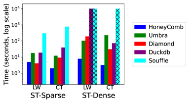
Figure 12. Performance on Tensor Dataset

Next, we compared HoneyComb with the baseline systems on tensor datasets using the queries LW (Loomis-Whitney) and CT (clover-triangle), which have more complex hypergraphs, typical for tensor kernels. The results, shown in Fig. 12, demonstrate that HoneyComb consistently outperforms most baselines across all queries and datasets, with significant runtime reductions in most cases. We do not include Kùzu, because it doesn’t support hypergraph queries. Thus, HoneyComb continues to outperform other systems on complex cyclic joins on $n$-ary ($n>2$) relations.

7.3. Scalability

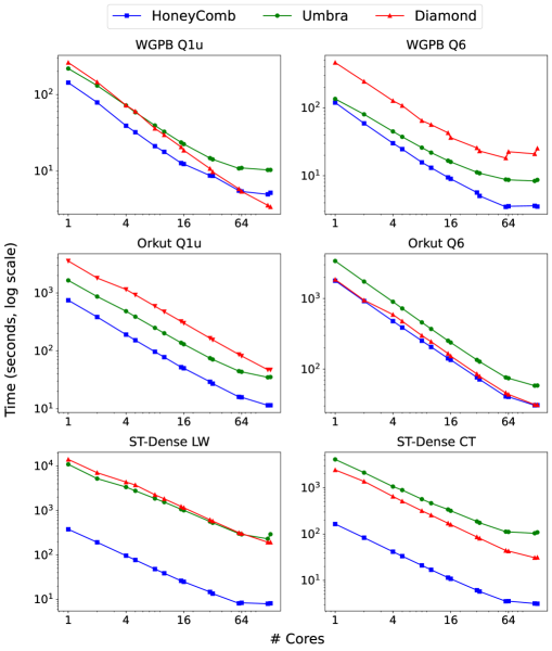
Figure 13. Speedup of query execution on $P=1,\ldots,120$ virtual cores (there are 60 hyperthreaded physical cores).

We evaluated HoneyComb’s scalability, by measuring the runtime of the system as a function of the number of virtual cores $P$. We report the findings only for HoneyComb, Umbra and Diamond, since other systems are generally too slow to show their scalability.

We tested the Q1u (triangle) and Q6 (4-clique) queries on the WGPB and Orkut dataset, as well as the LW (Loomis-Whitney) and CT (clover-triangle) queries on the ST-Dense Dataset.

The results are shown in Fig. 13. We find that HoneyComb consistently demonstrated almost linear scalability up to the maximum number of physical cores, which was 60 on our system. Increasing the number of virtual cores up to 120 led to no additional performance improvements at most cases, showing that the cores were saturated and the use of hyperthreads was not effective; we also confirmed that the CPUs were at almost 100 utilization at 60 virtual cores. In a few cases (Orkut), HoneyComb’s performance continued to improve a little beyond 60 cores: this is because of a higher contribution to the runtime of exponential search in middle loops, which is less memory efficient. Manually replacing exponential search with linear search restored full CPU utilization at 60 cores.

Umbra also shows an almost linear speedup, but slightly below that of HoneyComb. For instance, consider Q6 on WGPB, HoneyComb is $1.12\times$ faster than Umbra on 1 core, but $2.52\times$ faster on 60 cores, demonstrating that our techniques improve scalability as we increase the number of cores. This can be attributed to several factors. On sparse datasets, suboptimal partitioning of skewed data can lead to long-tail latencies, negatively impacting performance. On dense datasets, read-write conflicts caused by lazy trie building further hinder speedup when executing queries in parallel, as these conflicts introduce additional overhead that reduces the efficiency of parallel execution.

Diamond demonstrates similar scalability to Umbra up to 60 cores in most cases. However, Diamond maintains good scalability beyond 60 cores, indicating that hyperthreading benefits its performance. This is mainly due to the use of secondary hash tables over entire relations in Expand3, which are memory-latency bound due to random hash probes over large tables. Hyperthreading, with its separate register stacks and shared execution engine, helps mitigate this bottleneck. Nonetheless, while Diamond achieves speedups beyond 60 cores, its design does not fully address memory access latency, resulting in overall slower performance compared to our system. By leveraging the CoCo index and Adaptive Searching, HoneyComb achieves better cache locality and effectively utilizes the computational power of cores.

Also, HoneyComb does not achieve optimal speedup on sparse and skew datasets, even though it has better scalability. This is because the partitioning strategy of HoneyComb is not only targeted to relieve the skewness problem but also to avoid huge duplicated computation, as mentioned in Sec. 1, which may hurt the scalability.

Besides, the preprocessing time is not fully parallelized, and the overhead of preprocessing is not negligible in sparse cases.

These experiments also point to the importance of query rewriting for scalability. Still consider Q6 on WGPB. If we remove the query rewriting optimization, then HoneyComb is $0.91\times$ faster than Umbra (i.e. slower) on 1 core, and $1.15\times$ faster on 60 cores. Thus without rewriting HoneyComb gains very little over Umbra as $P$ increases (due to its mitigation of skew), but the gain becomes more pronounced when we enable the query rewriting optimization.

7.4. Variable Ordering

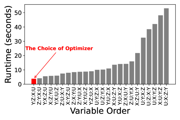
Figure 14. Effect of Variable Ordering

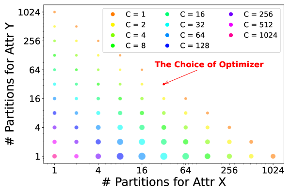
Figure 15. Effects of Partition Shares

Recall that the theoretical analysis of the worst-case optimal join holds for any choice of variable order, however, in practice, the choice of variable order may affect the runtime significantly. Next, we evaluated how much the variable order can affect the runtime of HoneyComb.

Fig. 15 shows the runtime for executing the Q6 (4-clique) query on WGPB, for all $24=4!$ possible variable orderings.

The results show that optimizing the variable order can have a significant impact on the query performance. This is because the order in which joins are executed directly influences the size of intermediate results, which can lead to substantial differences in both memory usage and computational effort.

Efficient ordering can minimize the number and length of intersections, reducing the overall complexity of the query execution. In contrast, poor ordering can result in intersecting large sets, which increases memory overhead and slows down execution.

To demonstrate the feasibility of our optimizer, we use a red bar to represent the ordering chosen by our optimizer in Fig. 15. In this particular Q6 (4-clique) query, our optimizer chooses the best variable order. This did not happen for all queries, but it is important to note that the optimizer does not need to select the absolute best ordering, as long as is not significantly slower than the optimal.

7.5. Partition

Next, we conducted a similar analysis on the choice of the partition shares. We ran the Q1u (triangle) query using $P=1024$ threads, and considered all possible ways to factorize it into $P=P_{X}\times P_{Y}\times P_{Z}$. The results are shown in Fig. 15: the $X$ and $Y$ axes show $P_{X},P_{Y}$ (the value of $P_{Z}$ can be inferred, and is also shown by the color of each dot), and the size of each dot represents the runtime (smaller is better). The optimal shares are $32\times 32\times 1$, and these are, indeed, the shares chosen by our optimizer. The traditional parallelization method, which allocates all shares to one variable, corresponds to the factorization $1024\times 1\times 1$, and is the right-most orange dot, which is visibly worse than the optimal choice of shares.

Recall that the HyperCube algorithm tries to minimize the communication cost; when all three relations of the query have the same size, then the optimal shares are equal, which, in our case corresponds to $8\times 8\times 16$ or some permutation thereof. As one can see from the graph, these choices of shares are far from optimal: our optimizer adjusts the partition shares based on not only the data distribution, but also on query characteristics that we care about. As noted in Sec. 6.3, the optimizer will rule out these partition shares by detecting the heavy duplicated intersection computations across different threads.

On the other hand, if we keep $P_{Z}=1$ then it doesn’t matter too much how many shares we allocate to $X$ or $Y$ (the line of red dots, which also contains the optimal configuration). This is because the data itself is relatively evenly distributed, and the difference in allocating shares between X and Y has little impact on performance.

Overall, the graph shows a large variation in the total runtime, proving the need for an optimized allocation of shares.

7.6. Query Rewriting and Indexes

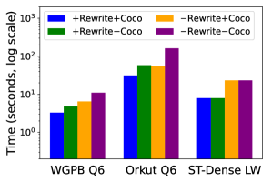
Figure 16. Effects of Rewriting and CoCo

In this section, we present additional experimental results that highlight key aspects of our optimization techniques.

We first evaluate the effectiveness of our query rewriting optimization by measuring the runtime with and without rewriting enabled. The results, summarized in Fig. 16, show that enabling query rewriting consistently improves performance across all queries. This demonstrates that our rewriting strategies optimize execution plans, leading to more efficient query processing. For the the queries LW on the ST-Dense dataset, the rewriting is not effective, due to no duplicated intersections in its plan.

Next, we assess the impact of our CoCo index on query performance. We compare the runtime with the CoCo index enabled and disabled, and the results indicate a significant performance improvement when the index is utilized. Also, we report the size of the CoCo index, which ranges from $1$GB to $5$GB for each table and is comparable with datasets. Thus, the CoCo does not introduce significant storage overhead. This ensures that the index remains practical for optimizing joins without imposing a large memory footprint.

In addition, we measure the total time spent in the preprocessing stage, which includes the creation of the CoCo index. The preprocessing time ranges from $0.2$s to $5$s, depending on the number of tables and the size of datasets. For long-running queries, the preprocessing time is generally minimal compared to the join execution time. For short-running queries, even sometimes the preprocessing time is larger than the join time, but the total runtime is still less than or comparable to other baselines. This indicates that the overhead introduced by preprocessing is acceptable, making our approach efficient and suitable for real-time query processing.

8. Conclusion

We introduced HoneyComb, an implementation of Generic Join (a special case of Worst Case Optimal Join) on a multicore, shared-memory architecture. Prior parallel implementations of WCOJ partitioned only the top loop variable. Instead, in HoneyComb we partition the domains of all variables, which reduces the computation skew. We also introduced a simple trie index, based on a novel two-stage sorting-based parallel algorithm, which can be constructed eagerly and cheaply, and removes concurrent conflicts during the query evaluation. The use of a sorted array instead of a hash table also takes advantage of modern hardware by improving cache locality and enabling vector processing. We co-optimized the choice of the variable order and the computation of the optimal shares by using a novel cost model for data skew, and described a rewriting technique for WCOJ that reduced the amount of redundant computations. Finally, we reported an extensive evaluation of our implementation, proving the effectiveness of the partitioning strategy, of the optimized choice of variable order and shares, and of the rewriting technique.

Future work includes further leveraging hardware by supporting vectorization, speeding up the optimization time through dynamic programming, and extending the rewriting technique to support more complicated cases.

References

- (1)
- wgp (2019) 2019. WGPB Dataset. https://zenodo.org/records/4035223. accessed October 2019.
- int (2021) 2021. Intel® oneAPI Threading Building Blocks. https://www.intel.com/content/www/us/en/developer/tools/oneapi/onetbb.html.
- kuz (2024) 2024. KÙZU Join Hint. https://docs.kuzudb.com/developer-guide/join-order-hint/.
- Aberger et al. (2016) Christopher R. Aberger, Susan Tu, Kunle Olukotun, and Christopher Ré. 2016. EmptyHeaded: A Relational Engine for Graph Processing. In Proceedings of the 2016 International Conference on Management of Data, SIGMOD Conference 2016, San Francisco, CA, USA, June 26 - July 01, 2016. ACM, 431–446.
- Abo Khamis et al. (2024) Mahmoud Abo Khamis, Vasileios Nakos, Dan Olteanu, and Dan Suciu. 2024. Join Size Bounds using lp-Norms on Degree Sequences. Proc. ACM Manag. Data 2, 2, Article 96 (may 2024), 24 pages. https://doi.org/10.1145/3651597
- Afrati and Ullman (2010) Foto N. Afrati and Jeffrey D. Ullman. 2010. Optimizing joins in a map-reduce environment. In EDBT 2010, 13th International Conference on Extending Database Technology, Lausanne, Switzerland, March 22-26, 2010, Proceedings (ACM International Conference Proceeding Series, Vol. 426). ACM, 99–110.
- Arch et al. (2022) Samuel Arch, Xiaowen Hu, David Zhao, Pavle Subotic, and Bernhard Scholz. 2022. Building a Join Optimizer for Soufflé. In Logic-Based Program Synthesis and Transformation - 32nd International Symposium, LOPSTR 2022, Tbilisi, Georgia, September 21-23, 2022, Proceedings (Lecture Notes in Computer Science, Vol. 13474), Alicia Villanueva (Ed.). Springer, 83–102. https://doi.org/10.1007/978-3-031-16767-6_5
- Aref et al. (2015) Molham Aref, Balder ten Cate, Todd J. Green, Benny Kimelfeld, Dan Olteanu, Emir Pasalic, Todd L. Veldhuizen, and Geoffrey Washburn. 2015. Design and Implementation of the LogicBlox System. In Proceedings of the 2015 ACM SIGMOD International Conference on Management of Data, Melbourne, Victoria, Australia, May 31 - June 4, 2015, Timos K. Sellis, Susan B. Davidson, and Zachary G. Ives (Eds.). ACM, 1371–1382. https://doi.org/10.1145/2723372.2742796
- Arroyuelo et al. (2021) Diego Arroyuelo, Aidan Hogan, Gonzalo Navarro, Juan L. Reutter, Javiel Rojas-Ledesma, and Adrián Soto. 2021. Worst-Case Optimal Graph Joins in Almost No Space. In SIGMOD ’21: International Conference on Management of Data, Virtual Event, China, June 20-25, 2021. ACM, 102–114.
- AWS (2024) AWS. 2024. Amazon EC2 High Memory (U-1) Instances. https://aws.amazon.com/ec2/instance-types/high-memory/. Accessed June 2024.
- Axtmann et al. (2017) Michael Axtmann, Sascha Witt, Daniel Ferizovic, and Peter Sanders. 2017. In-Place Parallel Super Scalar Samplesort (IPSSSSo). In 25th Annual European Symposium on Algorithms (ESA 2017) (Leibniz International Proceedings in Informatics (LIPIcs), Vol. 87). Schloss Dagstuhl–Leibniz-Zentrum fuer Informatik, 9:1–9:14. https://doi.org/10.4230/LIPIcs.ESA.2017.9
- Axtmann et al. (2020) Michael Axtmann, Sascha Witt, Daniel Ferizovic, and Peter Sanders. Sept. 2020. Engineering In-place (Shared-memory) Sorting Algorithms. Computing Research Repository (CoRR). arXiv:2009.13569
- Baeza-Yates and Salinger (2010) Ricardo Baeza-Yates and Alejandro Salinger. 2010. Fast Intersection Algorithms for Sorted Sequences. In Algorithms and Applications, Essays Dedicated to Esko Ukkonen on the Occasion of His 60th Birthday (Lecture Notes in Computer Science, Vol. 6060), Tapio Elomaa, Heikki Mannila, and Pekka Orponen (Eds.). Springer, 45–61. https://doi.org/10.1007/978-3-642-12476-1_3
- Beame et al. (2017) Paul Beame, Paraschos Koutris, and Dan Suciu. 2017. Communication Steps for Parallel Query Processing. J. ACM 64, 6 (2017), 40:1–40:58. https://doi.org/10.1145/3125644
- Birler et al. (2024) Altan Birler, Alfons Kemper, and Thomas Neumann. 2024. Robust Join Processing with Diamond Hardened Joins. Proc. VLDB Endow. 17, 11 (2024), 3215–3228. https://doi.org/10.14778/3681954.3681995
- Blanas et al. (2011) Spyros Blanas, Yinan Li, and Jignesh M. Patel. 2011. Design and evaluation of main memory hash join algorithms for multi-core CPUs. In Proceedings of the ACM SIGMOD International Conference on Management of Data, SIGMOD 2011, Athens, Greece, June 12-16, 2011, Timos K. Sellis, Renée J. Miller, Anastasios Kementsietsidis, and Yannis Velegrakis (Eds.). ACM, 37–48. https://doi.org/10.1145/1989323.1989328
- Boncz and Kersten (1999) Peter A. Boncz and Martin L. Kersten. 1999. MIL Primitives for Querying a Fragmented World. VLDB J. 8, 2 (1999), 101–119. https://doi.org/10.1007/S007780050076
- Brisaboa et al. (2015) Nieves R. Brisaboa, Ana Cerdeira-Pena, Antonio Fariña, and Gonzalo Navarro. 2015. A Compact RDF Store Using Suffix Arrays. In String Processing and Information Retrieval - 22nd International Symposium, SPIRE 2015, London, UK, September 1-4, 2015, Proceedings (Lecture Notes in Computer Science, Vol. 9309), Costas S. Iliopoulos, Simon J. Puglisi, and Emine Yilmaz (Eds.). Springer, 103–115. https://doi.org/10.1007/978-3-319-23826-5_11
- Buluç et al. (2009) Aydin Buluç, Jeremy T. Fineman, Matteo Frigo, John R. Gilbert, and Charles E. Leiserson. 2009. Parallel sparse matrix-vector and matrix-transpose-vector multiplication using compressed sparse blocks. In SPAA 2009: Proceedings of the 21st Annual ACM Symposium on Parallelism in Algorithms and Architectures, Calgary, Alberta, Canada, August 11-13, 2009, Friedhelm Meyer auf der Heide and Michael A. Bender (Eds.). ACM, 233–244. https://doi.org/10.1145/1583991.1584053
- Cai et al. (2019) Walter Cai, Magdalena Balazinska, and Dan Suciu. 2019. Pessimistic Cardinality Estimation: Tighter Upper Bounds for Intermediate Join Cardinalities. In Proceedings of the 2019 International Conference on Management of Data, SIGMOD Conference 2019, Amsterdam, The Netherlands, June 30 - July 5, 2019, Peter A. Boncz, Stefan Manegold, Anastasia Ailamaki, Amol Deshpande, and Tim Kraska (Eds.). ACM, 18–35. https://doi.org/10.1145/3299869.3319894
- Chou et al. (2018) Stephen Chou, Fredrik Kjolstad, and Saman P. Amarasinghe. 2018. Format abstraction for sparse tensor algebra compilers. Proc. ACM Program. Lang. 2, OOPSLA (2018), 123:1–123:30. https://doi.org/10.1145/3276493
- Chu et al. (2015) Shumo Chu, Magdalena Balazinska, and Dan Suciu. 2015. From Theory to Practice: Efficient Join Query Evaluation in a Parallel Database System. In Proceedings of the 2015 ACM SIGMOD International Conference on Management of Data, Melbourne, Victoria, Australia, May 31 - June 4, 2015. ACM, 63–78.
- DeWitt et al. (1990) David J. DeWitt, Shahram Ghandeharizadeh, Donovan A. Schneider, Allan Bricker, Hui-I Hsiao, and Rick Rasmussen. 1990. The Gamma Database Machine Project. IEEE Trans. Knowl. Data Eng. 2, 1 (1990), 44–62. https://doi.org/10.1109/69.50905
- DeWitt and Gray (1990) David J. DeWitt and Jim Gray. 1990. Parallel Database Systems: The Future of Database Processing or a Passing Fad? SIGMOD Rec. 19, 4 (1990), 104–112. https://doi.org/10.1145/122058.122071
- DeWitt and Gray (1992) David J. DeWitt and Jim Gray. 1992. Parallel Database Systems: The Future of High Performance Database Systems. Commun. ACM 35, 6 (1992), 85–98. https://doi.org/10.1145/129888.129894
- DeWitt et al. (1992) David J. DeWitt, Jeffrey F. Naughton, Donovan A. Schneider, and S. Seshadri. 1992. Practical Skew Handling in Parallel Joins. In 18th International Conference on Very Large Data Bases, August 23-27, 1992, Vancouver, Canada, Proceedings, Li-Yan Yuan (Ed.). Morgan Kaufmann, 27–40. http://www.vldb.org/conf/1992/P027.PDF
- Freitag et al. (2020a) Michael J. Freitag, Maximilian Bandle, Tobias Schmidt, Alfons Kemper, and Thomas Neumann. 2020a. Adopting Worst-Case Optimal Joins in Relational Database Systems. Proc. VLDB Endow. 13, 11 (2020), 1891–1904.
- Freitag et al. (2020b) Michael J. Freitag, Maximilian Bandle, Tobias Schmidt, Alfons Kemper, and Thomas Neumann. 2020b. Combining Worst-Case Optimal and Traditional Binary Join Processing. Technical Report TUM-I2082. Technische Universität München.
- Hogan et al. (2019) Aidan Hogan, Cristian Riveros, Carlos Rojas, and Adrián Soto. 2019. A Worst-Case Optimal Join Algorithm for SPARQL. In The Semantic Web - ISWC 2019 - 18th International Semantic Web Conference, Auckland, New Zealand, October 26-30, 2019, Proceedings, Part I (Lecture Notes in Computer Science, Vol. 11778), Chiara Ghidini, Olaf Hartig, Maria Maleshkova, Vojtech Svátek, Isabel F. Cruz, Aidan Hogan, Jie Song, Maxime Lefrançois, and Fabien Gandon (Eds.). Springer, 258–275. https://doi.org/10.1007/978-3-030-30793-6_15
- Hu (2021) Xiao Hu. 2021. Cover or Pack: New Upper and Lower Bounds for Massively Parallel Joins. In PODS’21: Proceedings of the 40th ACM SIGMOD-SIGACT-SIGAI Symposium on Principles of Database Systems, Virtual Event, China, June 20-25, 2021, Leonid Libkin, Reinhard Pichler, and Paolo Guagliardo (Eds.). ACM, 181–198. https://doi.org/10.1145/3452021.3458319
- Hu and Yi (2020) Xiao Hu and Ke Yi. 2020. Massively Parallel Join Algorithms. SIGMOD Rec. 49, 3 (2020), 6–17. https://doi.org/10.1145/3444831.3444833
- Jin et al. (2023) Guodong Jin, Xiyang Feng, Ziyi Chen, Chang Liu, and Semih Salihoglu. 2023. KÙZU Graph Database Management System. In 13th Conference on Innovative Data Systems Research, CIDR 2023, Amsterdam, The Netherlands, January 8-11, 2023. www.cidrdb.org. https://www.cidrdb.org/cidr2023/papers/p48-jin.pdf
- Khamis et al. (2024) Mahmoud Abo Khamis, Vasileios Nakos, Dan Olteanu, and Dan Suciu. 2024. Join Size Bounds using l-Norms on Degree Sequences. Proc. ACM Manag. Data 2, 2 (2024), 96. https://doi.org/10.1145/3651597
- Khamis et al. (2016) Mahmoud Abo Khamis, Hung Q. Ngo, and Atri Rudra. 2016. FAQ: Questions Asked Frequently. In Proceedings of the 35th ACM SIGMOD-SIGACT-SIGAI Symposium on Principles of Database Systems, PODS 2016, San Francisco, CA, USA, June 26 - July 01, 2016, Tova Milo and Wang-Chiew Tan (Eds.). ACM, 13–28. https://doi.org/10.1145/2902251.2902280
- Kjolstad et al. (2017) Fredrik Kjolstad, Shoaib Kamil, Stephen Chou, David Lugato, and Saman P. Amarasinghe. 2017. The tensor algebra compiler. Proc. ACM Program. Lang. 1, OOPSLA (2017), 77:1–77:29. https://doi.org/10.1145/3133901
- Koutris et al. (2016) Paraschos Koutris, Paul Beame, and Dan Suciu. 2016. Worst-Case Optimal Algorithms for Parallel Query Processing. In 19th International Conference on Database Theory, ICDT 2016, Bordeaux, France, March 15-18, 2016 (LIPIcs, Vol. 48). Schloss Dagstuhl - Leibniz-Zentrum für Informatik, 8:1–8:18.
- Koutris et al. (2018) Paraschos Koutris, Semih Salihoglu, and Dan Suciu. 2018. Algorithmic Aspects of Parallel Data Processing. Found. Trends Databases 8, 4 (2018), 239–370. https://doi.org/10.1561/1900000055
- Koutris and Suciu (2016) Paraschos Koutris and Dan Suciu. 2016. A Guide to Formal Analysis of Join Processing in Massively Parallel Systems. SIGMOD Rec. 45, 4 (2016), 18–27.
- Leskovec et al. (2005) Jure Leskovec, Jon M. Kleinberg, and Christos Faloutsos. 2005. Graphs over time: densification laws, shrinking diameters and possible explanations. In Proceedings of the Eleventh ACM SIGKDD International Conference on Knowledge Discovery and Data Mining, Chicago, Illinois, USA, August 21-24, 2005, Robert Grossman, Roberto J. Bayardo, and Kristin P. Bennett (Eds.). ACM, 177–187. https://doi.org/10.1145/1081870.1081893
- McAuley and Leskovec (2012) Julian J. McAuley and Jure Leskovec. 2012. Learning to Discover Social Circles in Ego Networks. In Advances in Neural Information Processing Systems 25: 26th Annual Conference on Neural Information Processing Systems 2012. Proceedings of a meeting held December 3-6, 2012, Lake Tahoe, Nevada, United States, Peter L. Bartlett, Fernando C. N. Pereira, Christopher J. C. Burges, Léon Bottou, and Kilian Q. Weinberger (Eds.). 548–556. https://proceedings.neurips.cc/paper/2012/hash/7a614fd06c325499f1680b9896beedeb-Abstract.html
- Mhedhbi and Salihoglu (2019) Amine Mhedhbi and Semih Salihoglu. 2019. Optimizing Subgraph Queries by Combining Binary and Worst-Case Optimal Joins. Proc. VLDB Endow. 12, 11 (2019), 1692–1704. https://doi.org/10.14778/3342263.3342643
- Mislove et al. (2007) Alan Mislove, Massimiliano Marcon, P. Krishna Gummadi, Peter Druschel, and Bobby Bhattacharjee. 2007. Measurement and analysis of online social networks. In Proceedings of the 7th ACM SIGCOMM Internet Measurement Conference, IMC 2007, San Diego, California, USA, October 24-26, 2007, Constantine Dovrolis and Matthew Roughan (Eds.). ACM, 29–42. https://doi.org/10.1145/1298306.1298311
- Ngo et al. (2013) Hung Q. Ngo, Christopher Ré, and Atri Rudra. 2013. Skew strikes back: new developments in the theory of join algorithms. SIGMOD Rec. 42, 4 (2013), 5–16. https://doi.org/10.1145/2590989.2590991
- Raasveldt and Mühleisen (2020) Mark Raasveldt and Hannes Mühleisen. 2020. Data Management for Data Science - Towards Embedded Analytics. In 10th Conference on Innovative Data Systems Research, CIDR 2020, Amsterdam, The Netherlands, January 12-15, 2020, Online Proceedings. www.cidrdb.org. http://cidrdb.org/cidr2020/papers/p23-raasveldt-cidr20.pdf
- Salihoglu (2023) Semih Salihoglu. 2023. Kùzu: A Database Management System For ”Beyond Relational” Workloads. SIGMOD Rec. 52, 3 (2023), 39–40. https://doi.org/10.1145/3631504.3631514
- Shahvarani and Jacobsen (2020) Amirhesam Shahvarani and Hans-Arno Jacobsen. 2020. Parallel Index-based Stream Join on a Multicore CPU. In Proceedings of the 2020 International Conference on Management of Data, SIGMOD Conference 2020, online conference [Portland, OR, USA], June 14-19, 2020, David Maier, Rachel Pottinger, AnHai Doan, Wang-Chiew Tan, Abdussalam Alawini, and Hung Q. Ngo (Eds.). ACM, 2523–2537. https://doi.org/10.1145/3318464.3380576
- Veldhuizen (2014) Todd L. Veldhuizen. 2014. Triejoin: A Simple, Worst-Case Optimal Join Algorithm. In Proc. 17th International Conference on Database Theory (ICDT), Athens, Greece, March 24-28, 2014, Nicole Schweikardt, Vassilis Christophides, and Vincent Leroy (Eds.). OpenProceedings.org, 96–106.
- Wang et al. (2023a) Junxiong Wang, Immanuel Trummer, Ahmet Kara, and Dan Olteanu. 2023a. ADOPT: Adaptively Optimizing Attribute Orders for Worst-Case Optimal Join Algorithms via Reinforcement Learning. Proc. VLDB Endow. 16, 11 (2023), 2805–2817. https://doi.org/10.14778/3611479.3611489
- Wang et al. (2023b) Yisu Remy Wang, Max Willsey, and Dan Suciu. 2023b. Free Join: Unifying Worst-Case Optimal and Traditional Joins. Proc. ACM Manag. Data 1, 2 (2023), 150:1–150:23. https://doi.org/10.1145/3589295
- Wu et al. (2022) Jiacheng Wu, Jin Wang, and Carlo Zaniolo. 2022. Optimizing Parallel Recursive Datalog Evaluation on Multicore Machines. In SIGMOD ’22: International Conference on Management of Data, Philadelphia, PA, USA, June 12 - 17, 2022, Zachary G. Ives, Angela Bonifati, and Amr El Abbadi (Eds.). ACM, 1433–1446. https://doi.org/10.1145/3514221.3517853
- Yin et al. (2017) Hao Yin, Austin R. Benson, Jure Leskovec, and David F. Gleich. 2017. Local Higher-Order Graph Clustering. In Proceedings of the 23rd ACM SIGKDD International Conference on Knowledge Discovery and Data Mining, Halifax, NS, Canada, August 13 - 17, 2017. ACM, 555–564. https://doi.org/10.1145/3097983.3098069
- Zhang et al. (2019) Shuhao Zhang, Jiong He, Amelie Chi Zhou, and Bingsheng He. 2019. BriskStream: Scaling Data Stream Processing on Shared-Memory Multicore Architectures. In Proceedings of the 2019 International Conference on Management of Data, SIGMOD Conference 2019, Amsterdam, The Netherlands, June 30 - July 5, 2019, Peter A. Boncz, Stefan Manegold, Anastasia Ailamaki, Amol Deshpande, and Tim Kraska (Eds.). ACM, 705–722. https://doi.org/10.1145/3299869.3300067
- Zhang et al. (2021) Shuhao Zhang, Yancan Mao, Jiong He, Philipp M. Grulich, Steffen Zeuch, Bingsheng He, Richard T. B. Ma, and Volker Markl. 2021. Parallelizing Intra-Window Join on Multicores: An Experimental Study. In SIGMOD ’21: International Conference on Management of Data, Virtual Event, China, June 20-25, 2021, Guoliang Li, Zhanhuai Li, Stratos Idreos, and Divesh Srivastava (Eds.). ACM, 2089–2101. https://doi.org/10.1145/3448016.3452793