iLOCO: Distribution-Free Inference for Feature Interactions

Abstract

Feature importance measures are widely studied and are essential for understanding model behavior, guiding feature selection, and enhancing interpretability. However, many machine learning fitted models involve complex, higher-order interactions between features. Existing feature importance metrics fail to capture these higher-order effects while existing interaction metrics often suffer from limited applicability or excessive computation; no methods exist to conduct statistical inference for feature interactions. To bridge this gap, we first propose a new model-agnostic metric, interaction Leave-One-Covariate-Out (iLOCO), for measuring the importance of higher-order feature interactions. Next, we leverage recent advances in LOCO inference to develop distribution-free and assumption-light confidence intervals for our iLOCO metric. To address computational challenges, we also introduce an ensemble learning method for calculating the iLOCO metric and confidence intervals that we show is both computationally and statistically efficient. We validate our iLOCO metric and our confidence intervals on both synthetic and real data sets, showing that our approach outperforms existing methods and provides the first inferential approach to detecting feature interactions.

Keywords: Interactions, feature importance, interpretability, minipatch ensembles, LOCO inference, distribution-free inference

1 Introduction

Machine learning systems are increasingly deployed in critical applications, necessitating human-understandable insights. Consequently, interpretable machine learning has become a rapidly expanding field [21, 8]. For predictive tasks, one of the most important aspects of interpretation is assessing feature importance. While much focus has been placed on quantifying the effects of individual features, the real power of machine learning lies in its ability to model higher-order interactions and complex feature representations [11]. However, there is a notable gap in interpretability: few methods provide insights into the higher-order interactions that truly drive model performance.

Understanding how features interact to influence predictions is a cornerstone of interpretable machine learning, particularly in applications requiring explainability. For instance, in genomics, interactions between genes can yield predictive insights into disease outcomes that individual genetic markers cannot. In drug discovery, uncovering how chemical properties interact can guide the identification of effective compounds in large-scale screening processes [25]. In material science, feature interactions reveal relationships that enable the development of innovative materials with desired properties. In business, analyzing interactions between customer demographics and purchasing behaviors can inform personalized marketing strategies and enhance customer retention [3].

In addition to detecting feature interactions, it is crucial to quantify the uncertainty associated with these interactions to ensure they are not simply noise. Uncertainty quantification has emerged as a focus in machine learning, addressing the need for more reliable and interpretable models [1]. While much of this work has traditionally centered on quantifying uncertainty in predictions [24], there has been a growing interest in extending these techniques to feature importance [33, 31]. To the best of our knowledge, there has been no uncertainty quantification or statistical inference studied for feature interaction importance.

Motivated by these challenges, we introduce the interaction Leave-One-Covariate-Out (iLOCO) metric and inference framework, which addresses key limitations of existing methods. Our framework provides a model-agnostic, distribution-free, statistically and computationally efficient solution for quantifying feature interactions and their uncertainties across diverse applications.

1.1 Related Works

There is an extensive body of literature on feature importance metrics [26, 2, 20, 21], but research on feature interactions is comparatively sparse. Shapley interaction values extend the game-theoretic concept of Shapley values to measure pairwise feature interactions, decomposing model predictions into main and interaction effects [28, 27, 23]. Similarly, the H-statistic, derived from partial dependence, quantifies the proportion of variance explained by feature interactions [9]. While these methods are theoretically well-grounded and model-agnostic, their computational complexity increases exponentially with the number of features, limiting their practical applicability.

Some approaches have been developed to detect and quantify interactions within specific model classes [4, 13], while other approaches focus on detecting the presence of interactions without providing a formal quantitative measure [14]. While these approaches can be effective, their insights may require manual inspection and interpretation, or may not generalize to other types of models.

There is a growing body of research on uncertainty quantification for feature importance [17, 16, 30, 31, 22]. However, to the best of our knowledge, no one has developed a technique for uncertainty quantification, specifically for feature interactions. Our goal is to develop confidence intervals for our feature interaction metric that reflect the statistical significance and uncertainty of this metric. Our method builds upon the Leave-One-Covariate-Out (LOCO) metric and inference framework originally proposed by [17]. Further, as computational considerations are a major challenge for interactions, we leverage the fast inference approach incorporating minipatches, simultaneous subsampling of observations and features, to enhance the computational efficiency of our approach.

1.2 Contributions

Our work focuses on two main contributions. First, we introduce iLOCO, a distribution-free, model-agnostic method for quantifying feature interactions that can be applied to any predictive model without relying on assumptions about the underlying data distribution. Moreover, we introduce an efficient way of estimating this metric via minipatch ensembles. Second, we develop rigorous distribution-free inference procedures for interaction effects, enabling confidence intervals for the interactions detected. Collectively, our contributions offer notable advancements in quantifying feature interaction importance and even higher-order interactions in interpretable machine learning.

2 iLOCO

2.1 Review: LOCO Metric

To begin, let us first review the widely used LOCO metric that is used for quantifying individual feature importance in predictive models [18]. For a feature $j$, LOCO measures its importance by evaluating the change in prediction error when the feature is excluded. Formally, given a prediction function $f:\mathcal{X}\to\mathbb{R}$ and an error measure $\text{Error}()$, the LOCO importance of feature $j$ is:

$$\Delta_{j}(\mathbf{X},\mathbf{Y})=\mathbb{E}\big{[}\text{Error}(Y,f^{-j}(X_{\setminus j};\mathbf{X}_{:,\setminus j},\mathbf{Y}))-\text{Error}(Y,f(X;\mathbf{X},\mathbf{Y}))\mid\mathbf{X},\mathbf{Y}\big{]},$$

where $f^{-j}$ is the prediction function trained without feature $j$. A large $\Delta_{j}$ value, which must be non-negative by definition, suggests the importance of the feature by indicating performance degradation when the feature is excluded. While LOCO is effective at measuring the importance of individual features, it has critical limitations in capturing feature interactions. If two features contribute to the prediction only when considered together, LOCO may fail to identify their joint importance, as the removal of a single feature might have minimal impact on the model’s performance. To address this challenge, the interaction LOCO (iLOCO) metric extends LOCO to explicitly account for pairwise feature interactions.

2.2 iLOCO Metric

Inspired by LOCO, we seek to define a score that measures the influence of the interaction of between two variables $j$ and $k$. Consider the expected difference in error between a further reduced model $f^{-j,k}$ and the full model:

$$\Delta_{j,k}(\mathbf{X},\mathbf{Y}) =\mathbb{E}[\operatorname{Error}(Y,f^{-j,k}(X_{\setminus\{j,k\}};\mathbf{X}_{:,\setminus\{j,k\}},\mathbf{Y})-\operatorname{Error}(Y,f(X;\mathbf{X},\mathbf{Y})\mid\mathbf{X},\mathbf{Y})]$$ (1)

The reduced model $f^{-j,k}$ removes covariates $j$ and $k$, their pairwise interaction, and any group involving $j$ or $k$. The quantity $\Delta_{j,k}$ captures the predictive power contributed by $j,k$ and all interactions that include them. This naturally leads to our iLOCO metric:

Definition 1.

For two features $j,k$, the iLOCO metric is defined as:

$$\text{iLOCO}_{j,k}=\Delta_{j}+\Delta_{k}-\Delta_{j,k}.$$ (2)

In particular, iLOCO finds the difference between the total influence of both $j$ and $k$ via $\Delta_{j}+\Delta_{k}$ and the influence specifically from $j$ and $k$ together, that is, $\Delta_{j,k}$. Our metric takes a similar form to that of the $H$-statistic [9]. A strong positive iLOCO metric indicates an important pairwise interaction.

To better understand and justify our proposed iLOCO metric, let us assume that the data generating model follows a functional ANOVA decomposition, a common assumption to quantify feature importance in interpretable machine learning [12, 19]. Specifically, suppose $f^{*}()$ can be decomposed into a sum of orthogonal functions with mean zero:

$$f^{*}(X) =g_{0}+\sum_{j=1}^{p}g_{j}(X_{j})+\sum_{1\leq j<k\leq p}g_{j,k}(X_{j},X_{k})+\sum_{1\leq j\leq k\leq l}g_{j,k,l}(X_{j},X_{k},X_{l})+\cdots.$$

which allows us to isolate the influence of each subset of variables. Suppose we define $\Delta^{*}_{j}$, $\Delta^{*}_{k}$, and $\Delta^{*}_{j,k}$ and the resulting $iLOCO^{*}_{j,k}$ based on this population model, $f^{*}()$. Then, in this population case and for a common classification error function, our metric directly isolates the contribution of the pairwise interaction term from the functional ANOVA decomposition:

Proposition 1.

Suppose $\text{Error}(Y,\hat{Y})=1-\hat{Y}$, then

$$iLOCO^{*}_{j,k}=g_{j,k}.$$

For other common error metrics like MSE, we show that our population iLOCO metric is proportional to $g_{j,k}$ in the functional ANOVA model; further details and proofs are given in the appendix. This illustrative population analysis shows that iLOCO directly captures the contributions of pairwise interactions.

Figure 1: Success probability of detecting feature pair $(1,2)$ across SNR levels for KRBF, RF, and MLP classifiers on nonlinear classification simulations (i), (ii), and (iii); the first feature pair has signal in scenarios (i) and (ii) whereas it is null in scenario (iii). Success probability is defined as the proportion of times the $(1,2)$ feature pair obtains the largest metric among all feature pairs. iLOCO-MP and iLOCO-Split consistently outperform existing approaches at detecting feature pair $(1,2)$ in the first two scenarios whereas iLOCO-MP exhibits superior specificity in the null scenario (iii).

2.3 iLOCO Estimation

To estimate our iLOCO metric in practice, we need access to new data samples to evaluate the expectation of the differences in prediction error. To this end, we introduce two estimation strategies, iLOCO via data-splitting and iLOCO via minipatch ensembles; the latter is specifically tailored to address the major computational burden that arises from fitting models leaving out all possible interactions.

iLOCO via Data Splitting
The data-splitting approach estimates iLOCO by partitioning the dataset $(\mathbf{X},\mathbf{Y})$ into a training set $D_{1}=(\mathbf{X}^{(1)},\mathbf{Y}^{(1)})$ and a test set $D_{2}=(\mathbf{X}^{(2)},\mathbf{Y}^{(2)})$. We train the full model $\hat{f}$ along with the models excluding $j$, $k$, and $j,k$ on training dataset $D_{1}$. The error functions for the full model and the corresponding feature-excluded error functions are evaluated on the test set $D_{2}$. This approach effectively computes iLOCO, but it comes with certain challenges. Since it involves training multiple models and only utilizes a subset of the dataset for each, there may be concerns about computational efficiency and the stability of the resulting metric.

iLOCO via Minipatches
To address the computational limitations of data splitting, we introduce iLOCO-MP (minipatches), an efficient estimation method that leverages ensembles of subsampled observations and features. This method repeatedly constructs minipatches by randomly sampling $n$ observations and $m$ features from the full dataset [32]. For each minipatch, a model is trained on the reduced dataset, and we can evaluate predictions on left-out observations. Specifically, for features $j$ and $k$, the leave-one-out and leave-two-covariates-out prediction is defined as $\hat{f}^{-j,k}_{-i}(X_{i})=\frac{1}{\sum_{b=1}^{B}\mathbb{I}(i\notin I_{b})\mathbb{I}(j,k\notin F_{b})}\sum_{b=1}^{B}\mathbb{I}(i\notin I_{b})\mathbb{I}(j,k\notin F_{b})\hat{f}_{b}(X_{i}),$ where $I_{b}\subset[N]$ is the set of observations selected for the $b$-th minipatch, $F_{b}\subset[M]$ is the set of features selected, $\hat{f}_{b}$ is the model trained on the minipatch, and $\mathbb{I}(\cdot)$ is an indicator function that checks whether an index is excluded. This formulation ensures that the predictions exclude both the observation $i$ and the features $j$ and $k$. We can define the other leave-one-out predictions accordingly to obtain a computationally efficient and stable approximation of the iLOCO metric. The full iLOCO-MP algorithm is given in the appendix. Note that the iLOCO-MP metric can only be computed for models in the form of minipatch ensembles built using any base model. Further, note that after fitting minipatch ensembles, computing the iLOCO metric requires no further model fitting and is nearly free computationally.

2.4 Extension to Higher-Order Interactions

Detecting higher-order feature interactions is crucial in understanding complex relationships in data, as many real-world phenomena involve intricate dependencies among multiple features that cannot be captured by pairwise interactions alone. To extend the iLOCO metric to account for such higher-order interactions, we generalize its definition to isolate the unique contributions of $S$-way interactions among features:

Definition 2.

For an $S$-way interaction, the iLOCO metric is defined as:

$$\text{iLOCO}_{S}=\sum_{T\subseteq S}(-1)^{|S|-|T|}\Delta_{T}.$$

Here, we sum over all possible subsets of $S$, and for each subset $T$, $\Delta_{T}$ denotes the contribution of $T$ to the model error. The term $(-1)^{|S|-|T|}$ alternates the sign based on the size of $T$, ensuring proper aggregation and cancellation of irrelevant terms that appear multiple times; further derivations and justification are given in the appendix. By leveraging this generalized formulation, iLOCO extends its ability to capture and quantify the contributions of higher-order interactions, providing a more complete understanding of complex feature relationships.

2.5 iLOCO for Correlated, Important Features

Quantifying the importance of correlated features is a known challenge and unsolved problem in interpretable machine learning [29]. This problem is especially pronounced for LOCO when correlated features are removed individually, the remaining correlated feature(s) can partially compensate, resulting in a small LOCO metric that can miss important, correlated features. Interestingly, our proposed iLOCO metric can solve this problem. Note that for a strongly correlated and important feature pair $j$ and $k$, $\Delta_{j}$ and $\Delta_{k}$ (and LOCO) will both be near zero as they compensate for each other. But, $\Delta_{j,k}$ will have a strong positive effect, and thus our iLOCO metric will be strongly negative for important, correlated feature pairs. Thus, our iLOCO metric can serve dual purposes: positive values indicate an important pairwise interaction whereas negative values indicate individually important but correlated feature pairs. Thus, this alternative application of iLOCO helps solve an important open problem in feature importance.

3 Distribution-Free Inference for iLOCO

Beyond just detecting interactions via our iLOCO metric, it is critical to quantify the uncertainty in these estimates to understand if they are significantly different than random noise. To address this, we develop distribution-free confidence intervals for both our iLOCO-Split and iLOCO-MP estimators that are valid under only mild assumptions.

3.1 iLOCO Inference via Data Splitting

As previously outlined, we can estimate the iLOCO metric via data splitting, where the training set $D_{1}$ is used for training predictive models $\hat{f},\,\hat{f}^{-j},\,\hat{f}^{-k},\,\hat{f}^{-j,k}$, while the test set $D_{2}$ with $N_{2}$ samples is used for evaluating the error functions for each trained model. Each test sample gives an unbiased estimate of the target iLOCO metric, $iLOCO^{\mathrm{split}}_{j,k}$, which is defined for the models trained on $(\boldsymbol{X}^{(1)},\,\boldsymbol{Y}^{(1)})$. Specifically, $iLOCO^{\mathrm{split}}_{j,k}=\Delta_{j}^{\mathrm{split}}+\Delta_{k}^{\mathrm{split}}-\Delta_{j,k}^{\mathrm{split}}$, where $\Delta_{j,k}^{\mathrm{split}}=\mathbb{E}[\mathrm{Error}(Y,\hat{f}^{-j,k}(X))-\mathrm{Error}(Y,\hat{f}(X))|\boldsymbol{X}^{(1)},\boldsymbol{Y}^{(1)}],$ and $\Delta_{j}^{\mathrm{split}}$, $\Delta_{k}^{\mathrm{split}}$ are defined similarly. Here, the expectation is taken over the unseen test data, conditioning on $D_{1}$, which is a slightly different inference target than defined in (2) which conditions on the model trained on all available data. To perform statistical inference for $iLOCO^{\mathrm{split}}_{j,k}$, one natural idea is to collect its estimates on all test samples $\{\widehat{iLOCO}_{j,k}(X_{i}^{(2)},Y_{i}^{(2)})\}_{i=1}^{N_{2}}$ and construct a confidence interval $\hat{\mathbb{C}}^{\mathrm{split}}_{j,k}$ based on a normal approximation. The detailed inference algorithm for iLOCO-Split is included in the appendix. First, we need the following assumption:

Assumption 1.

Assume a bounded third moment: $\mathbb{E}(\widehat{iLOCO}_{j,k}(X_{i}^{(2)},Y_{i}^{(2)})-iLOCO^{\mathrm{split}}_{j,k})^{3}/\sigma_{j,k}^{3}\leq C$, where $\sigma_{j,k}^{2}=\mathrm{Var}(\widehat{iLOCO}_{j,k}(X_{i}^{(2)},Y_{i}^{(2)})|\boldsymbol{X}^{(1)},\boldsymbol{Y}^{(1)})$.

Then, the following theorem guarantees valid asymptotic coverage of $\hat{\mathbb{C}}^{\mathrm{split}}_{j,k}$ for inference target $iLOCO^{\mathrm{split}}_{j,k}$.

Theorem 1 (Coverage of iLOCO-Split).

Suppose Assumption 7 holds and $\{(X_{i},Y_{i})\}_{i=1}^{N}$ are i.i.d., then we have $\lim_{N^{\mathrm{test}}\rightarrow\infty}\mathbb{P}(iLOCO^{\mathrm{split}}_{j,k}\in\mathbb{C}^{\mathrm{split}}_{j,k})=1-\alpha$.

3.2 iLOCO Inference via Minipatches

Recall that after fitting minipatch ensembles, estimating the iLOCO metric is computationally free, as estimates aggregate over left out observations and/or features. Such advantages also carry over to statistical inference. In particular, we aim to perform inference for the target iLOCO score defined in (2); note that this inference target is conditioned on all data instead of a random data split, $D_{1}$ as with iLOCO-Split. Then, for each sample $i$, we can compute the leave-one-observation-out predictors $\hat{f}_{-i}$, $\hat{f}_{-i}^{-j}$, $\hat{f}_{-i}^{-k}$, $\hat{f}_{-i}^{-j,k}$ simply by aggregating appropriate minipatch predictors, and evaluating these predictors on sample $i$ to obtain $\widehat{iLOCO}_{j,k}(X_{i},Y_{i})$. For statistical inference, we collect $\{\widehat{iLOCO}_{j,k}(X,Y)\}_{i=1}^{N}$ and construct a confidence interval $\mathbb{C}^{\mathrm{MP}}_{j,k}$ based on a normal approximation. The detailed inference procedure is given in the appendix.

Despite the fact that $\widehat{iLOCO}_{j,k}(X_{i},Y_{i})$ has a complex dependency structure since all the data is essentially used for both fitting and inference, we show asymptotically valid coverage of $\mathbb{C}^{\mathrm{MP}}_{j,k}$ under some mild assumptions. First, let $h_{j,k}(X,Y)=\mathbb{E}_{\boldsymbol{X},\boldsymbol{Y}}[\mathrm{Err}(Y,\hat{f}^{-j}(X_{-j}))+\mathrm{Err}(Y,\hat{f}^{-k}(X_{-k}))-\mathrm{Err}(Y,\hat{f}^{-j,-k}(X_{-j,-k}))-\mathrm{Err}(Y,\hat{f}(X))|X,Y]$ be the interaction importance score of feature pair $(j,k)$ evaluated at sample $(X,Y)$, with expectation taken over the training data $(\boldsymbol{X},\boldsymbol{Y})$ that gives rise to the predictive models. Also let $\sigma_{j,k}^{\mathrm{MP}}=\mathrm{Var}(h_{j,k}(X_{i},Y_{i}))$.

Assumption 2.

Assume a bounded third moment: $\mathbb{E}[h_{j,k}(X,\,Y)-\mathbb{E}h_{j,k}(X,\,Y)]^{3}/(\sigma^{\mathrm{MP}}_{j,k})^{3}\leq C$.

Assumption 3.

The error function is Lipschitz continuous w.r.t. the prediction: for any $Y\in\mathbb{R}$ and any predictions $\hat{Y}_{1},\,\hat{Y}_{2}\in\mathbb{R}^{d}$, $|\mathrm{Error}(Y,\hat{Y}_{1})-\mathrm{Error}(Y,\hat{Y}_{2})|\leq L\|\hat{Y}_{1}-\hat{Y}_{2}\|_{2}$.

Common error functions like $\text{Error}(Y,\hat{Y})=1-\hat{Y}$ for classification or mean absolute error for regression both trivially satisfy this assumption.

Assumption 4.

The prediction difference between the predictors trained on different minipatches are bounded by $D$ at any input value $X$.

Assumption 5.

The minipatch sizes $(m,\,n)$ satisfy $\frac{m}{M},\,\frac{n}{N}\leq\gamma$ for some constant $0<\gamma<1$, and $n=o(\frac{\sigma_{j,k}^{\mathrm{MP}}}{LD}\sqrt{N})$.

Assumption 6.

The number of minipatches satisfies $B\gg(\frac{D^{2}L^{2}N}{(\sigma_{j,k}^{\mathrm{MP}})^{2}}+1)\log N$.

These are mild assumptions on the minipatch size and number. Further, note that predictions between any pair of minipatches must simply be bounded, which is a much weaker condition that stability conditions typical in the distribution-free inference literature [15].

Theorem 2 (Coverage of iLOCO-MP).

Suppose Assumptions 8-12 hold and $\{(X_{i},Y_{i})\}_{i=1}^{N}$ i.i.d., then we have $\lim_{N\rightarrow\infty}\mathbb{P}(iLOCO^{\mathrm{MP}}_{j,k}\in\mathbb{C}^{\mathrm{MP}}_{j,k})=1-\alpha$.

The detailed theorems, assumptions, and proofs can be found in the appendix. Note that the proof follows closely from that of [35], with the addition of a third moment condition to imply uniform integrability. Overall, our work has provided the first model-agnostic and distribution-free inference procedure for feature interactions that is asymptomatically valid under mild assumptions. Further, note that while iLOCO inference via minipatches requires utilizing minipatch ensemble predictors, it gains in both statistical and computational efficiency as it does not require data splitting and conducting inference conditional on only a random portion of the data.

4 Empirical Studies

4.1 Simulation Setup and Results

We design simulation studies to validate our proposed iLOCO metric and the corresponding inference procedure. We generate data $X_{i}\stackrel{{\scriptstyle i.i.d}}{{\sim}}N(0,\mathbf{I})$ and let $M=10$ and $N=500$ in our base simulations. We consider three major simulation scenarios for classification and regression as well as linear and non-linear settings: (i) $f(\mathbf{X})=snr\cdot(X_{1}\cdot X_{2})+\mathbf{X}\boldsymbol{\beta}$, (ii) $f(\mathbf{X})=snr\cdot(X_{1}\cdot X_{2})+(X_{2}\cdot X_{3})+(X_{3}\cdot X_{4})+(X_{4}\cdot X_{5})+\mathbf{X}\boldsymbol{\beta}$, and (iii) $f(\mathbf{X})=snr\cdot(X_{1}\cdot X_{2}\cdot X_{3})+\mathbf{X}\boldsymbol{\beta}$. Here, $\beta_{j}\sim N(2,0.5)$ for $j=1,\dots,5$, and $\beta_{j}=0$ for $j=6,\dots,10$ and as we are primary interested in detecting the first feature interaction, we let $snr$ denote the signal strength of the interaction. For non-linear simulations, we modify the interaction terms in $f(\mathbf{X})$ by applying a hyperbolic tangent transformation ($\tanh$) to all products. For regression scenarios, we let $Y=f(\mathbf{X})+\epsilon$ where $\epsilon\stackrel{{\scriptstyle i.i.d.}}{{\sim}}N(0,1)$, and for classification scenarios, we employ a logistic model with $Y\stackrel{{\scriptstyle i.i.d.}}{{\sim}}Bern(\sigma(f(\mathbf{X})))$, where $\sigma$ is the sigmoid function. In our simulations, we set the number of minipatches for iLOCO-MP to be $B=10,000$ and the minipatch size to be $m=20\%M$ and $n=20\%N$; for iLOCO-Split, we utilize 50% of samples for training and 50% for evaluating the predictions or inference. several baselines including the H-Statistic [9], FaithShap [28], Iterative Forest[4], and our proposed metrics iLOCO-split and iLOCO-MP. We report the success probability, which is defined as the proportion of times the (1,2) feature pair obtains the largest metric among all feature pairs. We report the success probability instead of the raw metric to enable consistent comparisons across methods and calibrate feature pair importance relative to others.

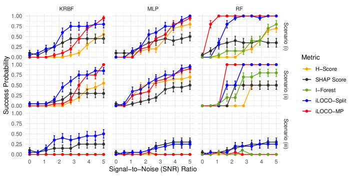
Figure A3: Success probability of detecting feature pair $(1,2)$ across SNR levels for KRBF, RF, and MLP regressors on linear regression simulations (i), (ii), and (iii)

We begin by evaluating iLOCO’s ability to capture the influence of a single feature pair across our aforementioned simulations. Figure A3 presents the success probability for detecting feature (1,2) averaged over 20 replicates across SNR levels for kernel radius basis function (KRBF), random forest (RF), and multilayer perception (MLP) regressors on non-linear classification simulations (i), (ii), (iii). The first two rows of Figure A3 illustrate simulations (i) and (ii). In these cases, we would expect the success probability of detecting feature pair (1,2) to increase as the SNR increases because the first feature pair has signal in these scenarios. As shown, iLOCO-Split (blue) and iLOCO-MP (red) consistently achieve the highest success probabilities compared to other metrics, demonstrating that our proposed metric more effectively captures feature interactions than the baselines. Notably, the success probability for Faith-Shap (black) does not always start at 0 when SNR= 0, indicating that Faith-Shap may not be well-calibrated relative to other feature pairs. In contrast, simulation (iii), which involves a tertiary interaction, should have a different outcome because feature pair (1,2) is null in this scenario. Indeed, we observe that the success probabilities for H-Score (yellow), I-Forest (green), and iLOCO-MP (red) remain near zero, aligning with expectations. However, Faith-Shap (black) and iLOCO-Split (blue) show success probabilities hovering around 0.25. For iLOCO-Split, this may be due to the reduced stability caused by splitting the data into training and test subsets, especially when the sample size ($N$) is smaller. Additionally, as noted earlier, Faith-Shap’s behavior suggests it is not well-calibrated. Additional simulation results for linear and linear, classification and regression, correlated features with $\boldsymbol{\Sigma}\neq\mathbf{I}$, and different minipatch sizes are in the appendix.

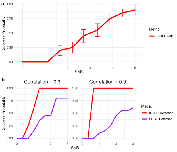
Figure 2: Panel (a) shows the success probability of detecting feature triple (1,2,3) for simulation (iii) using KRBF regressor and our higher-order extension of the iLOCO metric (estimated via iLOCO-MP). Panel (b) shows the success probability of detecting correlated, important feature pair (1,2). The success probability for iLOCO detection is defined as the proportion of times iLOCO _1,2 is the most negative amongst all pairs at each SNR value. For the LOCO detection, the success probability is defined as the proportion of times LOCO for both features 1 and 2 obtain the highest two values compared to all other features at each SNR. This validates that negative values of our iLOCO are able to identify features that are both correlated and important, and that are missed by existing feature importance metrics.

Table 1: Timing results (seconds) for various dataset sizes using Simulation 1 and the KRBF regressor for all methods except Iterative Forest, where RF regressor was used. As $M$ and $N$ grow, computing interaction importance scores using H-Statistic and Faith Shap becomes infeasible. Note that the (p) indicates the code for that method was distributed across multiple processes.

Method	$N$ = 250, $M$ = 10	$N$ = 500, $M$ = 20	$N$ = 1000, $M$ = 100	N = 10000, M = 500
H-Statistic	285.4	97201.2	$>$ 6 days	$>$ 6 days
Faith-Shap	70.2	72801.3	$>$ 6 days	$>$ 6 days
Iterative Forest	14.1	17.8	20.3	76.8
iLOCO Data Splitting	16.8 (p)	144.7 (p)	738.3 (p)	5481.2 (p)
iLOCO MP	24.3 (p)	27.2 (p)	38.7 (p)	193.5 (p)

In Figure 2, we validate iLOCO’s extensions. We first validate iLOCO’s ability to extend to higher-order interactions by computing $\text{iLOCO}_{j,k,\ell}$ on simulation (iii) using a KRBF regressor to capture the tertiary interaction among features (1, 2, 3). Figure 2a illustrates the success probability of detecting this feature trio using iLOCO-MP. We employ $B=50,000$ minipatches to account for the increased complexity and interaction space when evaluating three-way feature relationships. As the SNR increases, iLOCO-MP successfully detects the tertiary interaction nearly 90% of the time, validating that iLOCO properly extends to higher-order interactions. We also evaluate iLOCO’s ability to detect features that are both important and correlated. Figure 2b shows the success probability of detecting the correlated, important feature pair $(1,2)$ for a KRBF regression model. In this setup, we let $f(\mathbf{X})=\mathbf{X}\boldsymbol{\beta}$, and features are correlated ($\Sigma_{1,2}=0.3$ or $\Sigma_{1,2}=0.9$). Here, SNR denotes $\beta_{1}=\beta_{2}$. Success probability for LOCO is the proportion of times features 1 and 2 rank highest, while for iLOCO, it is the proportion where iLOCO _1,2 is the most negative. As SNR increases, iLOCO consistently detects correlated, important features, unlike LOCO, which often fails. This effect becomes more pronounced with stronger correlations.

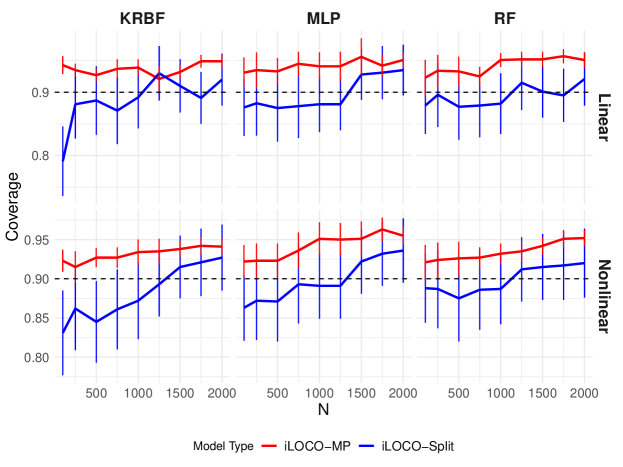
Figure 3: Coverage of 90% confidence intervals for a null feature pair in synthetic regression simulation (i) using KRBF, MLP, and RF as the base estimators. iLOCO-MP exhibits slight over-coverage whereas iLOCO-Split has valid coverage greater 0.9 for sufficiently large sample size; this validates of inferential theory.

Additionally, we construct an empirical study to demonstrate that the interaction feature importance confidence intervals generated by iLOCO-MP and iLOCO-Split have valid coverage for the inference target. Since the exact value of the inference target iLOCO involves expectation and hence is hard to compute, we use Monte Carlo approximation with 10,000 test data points and $B=10,000$ random minipatches. We evaluate the coverage and width of the confidence intervals constructed from 50 replicates. Figure A7 shows coverage rates for iLOCO-Split and iLOCO-MP of 90$\%$ confidence intervals for a null feature pair in regression simulation (i) using KRBF, MLP, and RF as the base estimators. iLOCO-MP exhibits slight overage-coverage whereas iLOCO-Split has valid coverage 0.9 for sufficiently large sample size, validating our inferential theory. We include additional studies where SNR = 2 in the appendix.

A key advantage of our iLOCO approach, particularly iLOCO-MP, is its exceptional computational efficiency. Table 1 compares the computational time required to calculate feature interaction metrics across all features in the dataset. Results are recorded on an Apple M2 Ultra 24-Core CPU at 3.24 GHz, 76-Core GPU, and 128GB of Unified Memory and across 11 processes when denoted using (p). As the dataset size ($N$) and the number of features ($M$) increase, methods like H-Statistic and Faith-Shap quickly become computationally infeasible. In contrast, iLOCO-MP shows significant efficiency gains, making it scalable to larger datasets without sacrificing performance. While Iterative Forest achieves reasonable computational times, it is restricted to random forest models. The efficiency and model-agnostic nature of iLOCO-MP highlight its practicality for real-world use cases involving complex datasets.

Figure 4: iLOCO (computed via iLOCO-MP) marginal confidence intervals ($\alpha=0.1$) on the Car Evaluation data (a) and Cocktail Recipe data (b). Confidence intervals that do not contain zero (blue dashed line) are statistically significant. Our inference procedure identifies meaningful, statistically significant interactions in both data sets, while also quantifying the uncertainty in our iLOCO metric.

4.2 Case Studies

We validate iLOCO by computing feature importance scores and intervals for two datasets. The Car Evaluation dataset with $N=1728$ and $M=15$ one-hot-encoded features seeks to predict car acceptability (classification task) [6]. We fit a minipatch forest model with 10,000 decision trees and a minipatch size of $m=20\%M$ and $n=20\%M$. Second, we gathered a new Cocktail Recipe dataset by web scrapping the Difford’s Guide website [7]. For our analysis, we consider the top $M=200$ most frequent one-hot-encoded ingredients for $N=15,972$ cocktails and the task is to predict the official Difford’s Guide ratings (regression task). We fit a kernel regressor with an RBF kernel with 30,000 minipatches, setting $m=50\%M$ and $n=50\%N$. In both cases, we set the error rate $\alpha=0.1$ and report marginal confidence intervals which control the False Coverage Rate [5]. In Figure 4, confidence intervals that do not contain zero (blue line) are deemed statistically significant.

In Figure 4a, we show the iLOCO-MP metric with confidence intervals for all feature pairs in the car evaluation dataset. Notably, the most important interactions include “medium price & low maintenance,” “4 doors & 5+ doors,” and “high maintenance & 3+ doors." These interactions suggest that the combination of price and maintenance level, as well as the number of doors, play a significant role in determining the car’s overall evaluation. For example, a medium price combined with low maintenance suggests an optimal trade-off between cost and upkeep, which could appeal to consumers. Interestingly, the interaction between “4 people & low safety" has a high iLOCO score but a lower bound below zero, indicating that while this combination might occasionally influence car acceptability, its contribution is not consistent across all cars.

Figure 4b shows the iLOCO-MP metric with confidence intervals for 40 ingredient interactions. iLOCO revealed two notable interactions: “Triple Sec & Agave Syrup" and “Coffee Liqueur & Espresso Coffee." The former likely reflects their complementary nature, as they are common pairings in popular cocktails such as margaritas. The latter pairing highlights the natural harmony between coffee elements, commonly found in popular espresso-based martinis. Interestingly, “Cranberry Juice & Black Raspberry Liqueur" exhibit a relatively high iLOCO score, likely due to their bold flavor combination blending tartness with rich berry notes. However, the higher degree of uncertainty may stem from variability in how drinkers perceive this pairing, as some may find it well-balanced while others see it as overpowering. Overall, these results emphasize the value of iLOCO and our inference procedure in detecting meaningful interactions between features and the importance of using confidence intervals to reflect the uncertainty in feature interactions.

5 Discussion

In this work, we propose iLOCO, a model-agnostic and distribution-free metric to quantify feature interactions. We also introduce the first inference procedure to construct confidence intervals to measure the uncertainty of feature interactions. Additionally, we propose a computationally fast way to estimate iLOCO and conduct inference using minipatch ensembles, allowing our approach to scale both computationally and statistically to large data sets. Our empirical studies demonstrate the superior ability of iLOCO to detect important feature interactions and highlight the important of uncertainty quantification in this context. We also briefly introduced using iLOCO to detect important correlated features as well as iLOCO for higher-order interactions, but future work could consider these important challenges further. Finally, for increasing numbers of features, detecting and testing pairwise and higher-order interactions becomes a major challenge. Future work could consider adaptive learning strategies, perhaps paired with minipatch ensembles [32], to focus both computational and statistical efforts on only the most important interactions in a large data set.

Inference Algorithms

Algorithm 1 iLOCO-Split Estimation and Inference

Input: Training data $(\boldsymbol{X}^{\rm{tr}},\boldsymbol{Y}^{\rm{tr}})$, test data $(\boldsymbol{X}^{\rm{test}},\boldsymbol{Y}^{\rm{test}})$, features $j,k$, base learners $H$.

1. Split the data into disjoint training and test sets: $(\boldsymbol{X}^{\rm{tr}},\boldsymbol{Y}^{\rm{tr}})$, $(\boldsymbol{X}^{\rm{test}},\boldsymbol{Y}^{\rm{test}})$.

2. Train prediction models $\hat{f}$, $\hat{f}^{-j}$, $\hat{f}^{-k}$, $\hat{f}^{-j,k}$ on $(\boldsymbol{X}^{\rm{tr}},\boldsymbol{Y}^{\rm{tr}})$:

   $$\begin{split}\hat{f}(X)=H(\boldsymbol{X}^{\rm{tr}},\boldsymbol{Y}^{\rm{tr}})(X),\quad\hat{f}^{-j}(X)=H(\boldsymbol{X}^{\rm{tr}}_{:,\backslash j},\boldsymbol{Y}^{\rm{tr}})(X_{\backslash j})\\ \hat{f}^{-k}(X)=H(\boldsymbol{X}^{\rm{tr}}_{:,\backslash k},\boldsymbol{Y}^{\rm{tr}})(X_{\backslash k}),\quad\hat{f}^{-j,k}(X)=H(\boldsymbol{X}^{\rm{tr}}_{:,\backslash j,k},\boldsymbol{Y}^{\rm{tr}})(X_{\backslash j,k})\end{split}$$

3. For the $i$th sample in the test set, compute the feature importance score and interaction score as follows:

   $$\hat{\Delta}_{j}(X^{\mathrm{test}}_{i},Y^{\mathrm{test}}_{i})=\text{Error}(Y^{\mathrm{test}}_{i},\hat{f}^{-j}(X^{\mathrm{test}}_{i}))-\text{Error}(Y^{\mathrm{test}}_{i},\hat{f}(X^{\mathrm{test}}_{i})),$$

   $$\hat{\Delta}_{k}(X^{\mathrm{test}}_{i},Y^{\mathrm{test}}_{i})=\text{Error}(Y^{\mathrm{test}}_{i},\hat{f}^{-k}(X^{\mathrm{test}}_{i}))-\text{Error}(Y^{\mathrm{test}}_{i},\hat{f}(X^{\mathrm{test}}_{i})),$$

   $$\hat{\Delta}_{j,k}(X^{\mathrm{test}}_{i},Y^{\mathrm{test}}_{i})=\text{Error}(Y^{\mathrm{test}}_{i},\hat{f}^{-j,k}(X^{\mathrm{test}}_{i}))-\text{Error}(Y^{\mathrm{test}}_{i},\hat{f}(X^{\mathrm{test}}_{i})).$$

4. Calculate iLOCO Metric for each sample $i$:

   $$\widehat{iLOCO}_{j,k}(X^{\mathrm{test}}_{i},Y^{\mathrm{test}}_{i})=\hat{\Delta}_{j}(X^{\mathrm{test}}_{i},Y^{\mathrm{test}}_{i})+\hat{\Delta}_{k}(X^{\mathrm{test}}_{i},Y^{\mathrm{test}}_{i})-\hat{\Delta}_{j,k}(X^{\mathrm{test}}_{i},Y^{\mathrm{test}}_{i}).$$

5. Let $N_{\mathrm{test}}$ be the sample size of the test data. Obtain a $1-\alpha$ confidence Interval for $iLOCO_{j,k}$:

   $$\mathbb{C}^{\mathrm{split}}_{j,k}=\left[\overline{iLOCO}_{j,k}-\frac{Z_{\alpha/2\hat{\sigma}_{j,k}}}{\sqrt{N_{\mathrm{test}}}},\overline{iLOCO}_{j,k}+\frac{Z_{\alpha/2\hat{\sigma}_{j,k}}}{\sqrt{N_{\mathrm{test}}}}\right],$$

   with
   

   $$\overline{iLOCO}_{jk}=\frac{1}{N_{\mathrm{test}}}\sum_{i=1}^{N_{\mathrm{test}}}\widehat{iLOCO}_{jk}(X^{\mathrm{test}}_{i},Y^{\mathrm{test}}_{i})$$

   being the sample mean and

   $$\hat{\sigma}_{j,k}=\sqrt{\frac{\sum_{i=1}^{N_{\mathrm{test}}}(\widehat{iLOCO}_{jk}(X^{\mathrm{test}}_{i},Y^{\mathrm{test}}_{i})-\overline{iLOCO}_{j,k})^{2}}{N_{\mathrm{test}}-1}}$$

   being the sample standard deviation.

Output: $\mathbb{C}^{\mathrm{split}}_{j,k}$

Algorithm 2 iLOCO-MP Estimation and Inference

Input: Training pairs $(\mathbf{X},\mathbf{Y})$, features $j,k$, minipatch sizes $n,m$, number of minipatches $B$, base learners $H$.

1. Perform Minipatch Learning: for $k=1,\dots,B$

   • Randomly subsample $n$ observations $I_{b}\subset[N]$ and $M$ features $F_{b}\subset[M]$.

   • Train prediction model $\hat{f}_{b}$ on $(\mathbf{X}_{I_{b},F_{b}},\mathbf{Y}_{I_{b}})$: $\hat{f}_{b}(X)=H(\mathbf{X}_{I_{b},F_{b}},\mathbf{Y}_{I_{b}})(X_{F_{b}}).$

2. Obtain predictions: LOO prediction:

   $$\hat{f}_{-i}(X_{i})=\\ \frac{1}{\sum_{b=1}^{B}\mathbb{I}(i\notin I_{b})}\sum_{b=1}^{B}\mathbb{I}(i\notin I_{b})\hat{f}_{b}(X_{i}).$$

   LOO + LOCO prediction (feature $j$):

   $$\hat{f}^{-j}_{-i}(X_{i})=\\ \frac{1}{\sum_{b=1}^{B}\mathbb{I}(i\notin I_{b})\mathbb{I}(j\notin F_{b})}\sum_{b=1}^{B}\mathbb{I}(i\notin I_{b})\mathbb{I}(j\notin F_{b})\hat{f}_{b}(X_{i}).$$

   LOO + $\text{LOCO}_{2}$ prediction (features $j,k$):

   $$\hat{f}^{-j,-k}_{-i}(X_{i})=\\ \frac{1}{\sum_{b=1}^{B}\mathbb{I}(i\notin I_{b})\mathbb{I}(j,k\notin F_{b})}\sum_{b=1}^{B}\mathbb{I}(i\notin I_{b})\mathbb{I}(j,k\notin F_{b})\hat{f}_{b}(X_{i}).$$

3. Calculate LOO Feature Occlusion:

   $$\hat{\Delta}_{j}(X_{i},Y_{i})=\text{Error}(Y_{i},\hat{f}^{-j}_{-i}(X_{i}))-\text{Error}(Y_{i},\hat{f}_{-i}(X_{i})),$$

   $$\hat{\Delta}_{k}(X_{i},Y_{i})=\text{Error}(Y_{i},\hat{f}^{-k}_{-i}(X_{i}))-\text{Error}(Y_{i},\hat{f}_{-i}(X_{i})),$$

   $$\hat{{\Delta}}_{j,k}(X_{i},Y_{i})=\text{Error}(Y_{i},\hat{f}^{-j,-k}_{-i}(X_{i}))-\text{Error}(Y_{i},\hat{f}_{-i}(X_{i})).$$

4. Calculate iLOCO Metric for each sample $i$:

   $$\widehat{iLOCO}_{j,k}(X_{i},Y_{i})=\hat{\Delta}_{j}(X_{i},Y_{i})+\hat{\Delta}_{k}(X_{i},Y_{i})-\hat{\Delta}_{j,k}(X_{i},Y_{i}).$$

5. Obtain a $1-\alpha$ confidence Interval for $iLOCO_{j,k}$: $\mathbb{C}^{\mathrm{MP}}_{j,k}=\left[\overline{iLOCO}_{j,k}-\frac{Z_{\alpha/2\hat{\sigma}_{j,k}}}{\sqrt{N}},\overline{iLOCO}_{j,k}+\frac{Z_{\alpha/2\hat{\sigma}_{j,k}}}{\sqrt{N}}\right]$, with
   $\overline{iLOCO}_{jk}=\frac{1}{N}\sum_{i=1}^{N}\widehat{iLOCO}_{jk}(X_{i},Y_{i})$ being the sample mean and $\hat{\sigma}_{j,k}=\sqrt{\frac{\sum_{i=1}^{N}(\widehat{iLOCO}_{jk}(X_{i},Y_{i})-\overline{iLOCO}_{j,k})^{2}}{N-1}}$ being the sample standard deviation

Output: $\mathbb{C}^{\mathrm{MP}}_{j,k}$

Appendix A Inference Theory for iLOCO-Split

Assumption 7.

The normalized iLOCO score on a random test sample satisfies the third moment assumption: $\mathbb{E}(\widehat{iLOCO}_{j,k}(X_{i}^{\mathrm{test}},Y_{i}^{\mathrm{test}})-iLOCO^{\mathrm{split}}_{j,k})^{3}/(\sigma^{\mathrm{split}}_{j,k})^{3}\leq C$, where $(\sigma^{\mathrm{split}}_{j,k})^{2}=\mathrm{Var}(\widehat{iLOCO}_{j,k}(X_{i}^{\mathrm{test}},Y_{i}^{\mathrm{test}})|\boldsymbol{X}^{\mathrm{tr}},\boldsymbol{Y}^{\mathrm{tr}})$.

We require Assumption 7 to establish the central limit theorem for the iLOCO metrics evaluated on the test data. Prior theory on LOCO-Split [36] does not have this assumption, but they focus on a truncated linear predictor and consider injecting noise into the LOCO scores, which can imply a third moment assumption similar to Assumption 7.

Theorem 3 (Coverage of iLOCO-Split).

Suppose that data $(X_{i},Y_{i})\overset{i.i.d.}{\sim}\mathcal{P}$. Under Assumption 7, we have $\lim_{N\rightarrow\infty}\mathbb{P}(iLOCO^{\mathrm{split}}_{j,k}\in\mathbb{C}^{\mathrm{split}}_{j,k})=1-\alpha$.

Proof.

Recall our definition of $\widehat{iLOCO}_{j,k}(X_{i}^{\mathrm{test}},Y_{i}^{\mathrm{test}})$ in Algorithm 1:

$$\widehat{iLOCO}_{j,k}(X^{\mathrm{test}}_{i},Y^{\mathrm{test}}_{i})=\hat{\Delta}_{j}(X^{\mathrm{test}}_{i},Y^{\mathrm{test}}_{i})+\hat{\Delta}_{k}(X^{\mathrm{test}}_{i},Y^{\mathrm{test}}_{i})-\hat{\Delta}_{j,k}(X^{\mathrm{test}}_{i},Y^{\mathrm{test}}_{i}).$$

Since we have assumed that all samples of the test data $(X_{i}^{\mathrm{test}},Y_{i}^{\mathrm{test}})\overset{i.i.d.}{\sim}\mathcal{P}$, we note that $\mathbb{E}(\hat{\Delta}_{j}(X^{\mathrm{test}}_{i},Y^{\mathrm{test}}_{i})|\boldsymbol{X}^{\mathrm{tr}},\boldsymbol{Y}^{\mathrm{tr}})=\Delta_{j}^{\mathrm{split}}$, $\mathbb{E}(\hat{\Delta}_{k}(X^{\mathrm{test}}_{i},Y^{\mathrm{test}}_{i})|\boldsymbol{X}^{\mathrm{tr}},\boldsymbol{Y}^{\mathrm{tr}})=\Delta_{k}^{\mathrm{split}}$, $\mathbb{E}(\hat{\Delta}_{k}(X^{\mathrm{test}}_{i},Y^{\mathrm{test}}_{i})|\boldsymbol{X}^{\mathrm{tr}},\boldsymbol{Y}^{\mathrm{tr}})=\Delta_{j,k}^{\mathrm{split}}$, and hence

$$\mathbb{E}[\widehat{iLOCO}_{j,k}(X_{i}^{\mathrm{test}},Y_{i}^{\mathrm{test}})|\boldsymbol{X}^{\mathrm{tr}},\boldsymbol{Y}^{\mathrm{tr}}]=\Delta_{j}^{\mathrm{split}}+\Delta_{k}^{\mathrm{split}}-\Delta_{j,k}^{\mathrm{split}}=iLOCO^{\mathrm{split}}_{j,k}.$$

Furthermore, due to Assumption 7, the Lyapunov condition holds for $\widehat{iLOCO}_{j,k}(X_{i}^{\mathrm{test}},Y_{i}^{\mathrm{test}})-\mathbb{E}(\widehat{iLOCO}_{j,k}(X_{i}^{\mathrm{test}},Y_{i}^{\mathrm{test}})|\boldsymbol{X}^{\mathrm{tr}},\boldsymbol{Y}^{\mathrm{tr}})/\sigma_{j,k}^{\mathrm{split}}$, conditional on the training set $\boldsymbol{X}^{\mathrm{tr}},\boldsymbol{Y}^{\mathrm{tr}}$, and hence we can invoke the central limit theorem to obtain that

$$\frac{1}{\sigma^{\mathrm{split}}_{j,k}\sqrt{N^{\mathrm{test}}}}\sum_{i=1}^{N^{\mathrm{test}}}[\widehat{iLOCO}_{j,k}(X_{i}^{\mathrm{test}},Y_{i}^{\mathrm{test}})-iLOCO^{\mathrm{split}}_{j,k}]\overset{d.}{\rightarrow}\mathcal{N}(0,1).$$

Now, it remains to show the consistency of the variance estimate $\hat{\sigma}_{j,k}=\frac{1}{N^{\mathrm{test}}-1}\sum_{i=1}^{N^{\mathrm{test}}}(\widehat{iLOCO}(X_{i}^{\mathrm{test}},Y_{i}^{\mathrm{test}})-\overline{iLOCO})^{2}$ for $(\sigma^{\mathrm{split}}_{j,k})^{2}$.

Define the random variable $\xi_{N^{\mathrm{test}},i}=[\widehat{iLOCO}_{j,k}(X_{i}^{\mathrm{test}},Y_{i}^{\mathrm{test}})-iLOCO^{\mathrm{split}}_{j,k}]^{2}/(\sigma_{j,k}^{\mathrm{split}})^{2}$. We aim to show that $\frac{1}{N^{\mathrm{test}}-1}\sum_{i=1}^{N^{\mathrm{test}}}\xi_{N^{\mathrm{test}},i}\overset{p}{\rightarrow}1$. By Assumption 7, we have $\mathbb{E}|\xi_{N^{\mathrm{test}},i}|^{3/2}=o(\sqrt{N})$. This implies the uniform integrability of $\{\xi_{N^{\mathrm{test}},i}\}_{i}$:

$$\begin{split}\mathbb{E}[|\xi_{N^{\mathrm{test}},i}|\mathbb{I}(|\xi_{N^{\mathrm{test}},i}|>x)]\leq&[\mathbb{E}|\xi_{N^{\mathrm{test}},i}|^{3/2}]^{\frac{2}{3}}[\mathbb{P}(|\xi_{N^{\mathrm{test}},i}|>x)]^{1/3}\\ \leq&[\mathbb{E}|\xi_{N^{\mathrm{test}},i}|^{3/2}]^{\frac{2}{3}}[\frac{\mathbb{E}|\xi_{N^{\mathrm{test}},i}|}{x}]^{1/3}\\ =&C^{2/3}x^{-1/3},\end{split}$$

which converges to zero as $x\rightarrow\infty$. Here, we applied Holder’s inequality on the first line, and applied Assumption 7 on the last line. With the uniform integrability of $\xi_{N^{\mathrm{test}},i}$, we can follow the last part of the proof of Theorem 4 in [34], and show that

$$\frac{1}{N^{\mathrm{test}}}\sum_{i=1}^{N^{\mathrm{test}}}\xi_{N^{\mathrm{test}},i}-1\overset{p}{\rightarrow}0,$$

which then implies $\frac{1}{N^{\mathrm{test}}-1}\sum_{i=1}^{N^{\mathrm{test}}}\xi_{N^{\mathrm{test}},i}\overset{p}{\rightarrow}1$ as $N^{\mathrm{test}}\rightarrow\infty$, and hence $\hat{\sigma}_{j,k}/\sigma_{j,k}^{\mathrm{MP}}\overset{p}{\rightarrow}1$.

Therefore, by Slutsky’s theorem, we have

$$\frac{1}{\hat{\sigma}_{j,k}\sqrt{N^{\mathrm{test}}}}\sum_{i=1}^{N^{\mathrm{test}}}[\widehat{iLOCO}_{j,k}(X_{i}^{\mathrm{test}},Y_{i}^{\mathrm{test}})-iLOCO^{\mathrm{split}}_{j,k}]\overset{d.}{\rightarrow}\mathcal{N}(0,1),$$

which implies the asymptotically valid coverage of $\mathbb{C}^{\mathrm{split}}_{j,k}$ for $iLOCO_{j,k}^{\mathrm{split}}$. ∎

Appendix B Inference Theory for iLOCO-MP

Notations:

Let $h_{j,k}(X,Y;\boldsymbol{X},\boldsymbol{Y})=\mathrm{Error}(Y,\mu_{\backslash j}(X_{\backslash j};\boldsymbol{X}_{:,\backslash j},\boldsymbol{Y}))+\mathrm{Error}(Y,\mu_{\backslash k}(X_{\backslash k};\boldsymbol{X}_{:,\backslash k},\boldsymbol{Y}))-\mathrm{Error}(Y,\mu_{\backslash j,k}(X_{\backslash j,k};\boldsymbol{X}_{:,\backslash j,k},\boldsymbol{Y}))-\mathrm{Error}(Y,\mu(X;\boldsymbol{X},\boldsymbol{Y}))$ be the interaction importance score of feature pair $(j,k)$, when using the model trained on $(\boldsymbol{X},\boldsymbol{Y})$ to predict data $(X,Y)$. Recall our definition of the $iLOCO^{\mathrm{MP}}_{j,k}$, we can then write

$$iLOCO^{\mathrm{MP}}_{j,k}=\mathbb{E}_{X,\,Y}[h_{j,k}(X,\,Y;\boldsymbol{X},\,\boldsymbol{Y})|\boldsymbol{X},\,\boldsymbol{Y}],$$

where $(X,\,Y)$ is independent of the training data $(\boldsymbol{X},\,\boldsymbol{Y})$. Also define $h_{j,k}(X,\,Y)=\mathbb{E}_{\boldsymbol{X},\,\boldsymbol{Y}}[h_{j,k}(X,\,Y;\boldsymbol{X},\,\boldsymbol{Y})|X,Y]$, where the expectation is taken over the training but not test data. Under the notation in the main paper, $\widetilde{iLOCO}_{j,k}(X,Y)=h_{j,k}(X,Y)$. Its variance $\mathrm{Var}(h_{j,k}(X_{i},Y_{i}))$ is denoted by $(\sigma^{\mathrm{MP}}_{j,k})^{2}$. Let $\hat{h}_{j,k}(X_{i},Y_{i};\boldsymbol{X}_{\backslash i,:},\boldsymbol{Y}_{\backslash i})=\widehat{iLOCO}_{j,k}(X_{i},Y_{i})$, the estimated pairwise interaction importance score at sample $i$ in Algorithm 2. Let $\tilde{h}_{j,k}(X_{i},Y_{i};\boldsymbol{X}_{\backslash i,;},\boldsymbol{Y}_{\backslash i})=h_{j,k}(X_{i},Y_{i};\boldsymbol{X}_{\backslash i,;},\boldsymbol{Y}_{\backslash i})-h_{j,k}(X_{i},Y_{i})$. Denote the trained predictor on each minipatch $(I,F)$ by $\hat{\mu}_{I,F}(\cdot)$.

Assumption 8.

The normalized interaction importance r.v. satisfies the third moment condition: $\mathbb{E}[h_{j,k}(X,\,Y)-\mathbb{E}h_{j,k}(X,\,Y)]^{3}/(\sigma^{\mathrm{MP}}_{j,k})^{3}\leq C$.

Assumption 9.

The error function is Lipschitz continuous w.r.t. the prediction: for any $Y\in\mathbb{R}$ and any predictions $\hat{Y}_{1},\,\hat{Y}_{2}\in\mathbb{R}^{d}$,

$$|\mathrm{Error}(Y,\hat{Y}_{1})-\mathrm{Error}(Y,\hat{Y}_{2})|\leq L\|\hat{Y}_{1}-\hat{Y}_{2}\|_{2}.$$

Assumption 10.

The prediction difference between different minipatches are bounded: $\|\hat{\mu}_{I,F}(X)-\hat{\mu}_{I^{\prime},F^{\prime}}(X)\|_{2}\leq D$ for any $X$, any minipatches $I,\,I^{\prime}\subset[N]$, $F,\,F^{\prime}\subset[M]$.

Assumption 11.

The minipatch sizes $(m,\,n)$ satisfy $\frac{m}{M},\,\frac{n}{N}\leq\gamma$ for some constant $0<\gamma<1$, and $n=o(\frac{\sigma^{\mathrm{MP}}_{j,k}}{LD}\sqrt{N})$.

Assumption 12.

The minipatch size number satisfies $B\gg(\frac{D^{2}L^{2}N}{(\sigma^{\mathrm{MP}}_{j,k})^{2}}+1)\log N$.

Theorem 4 (Coverage of iLOCO-MP).

Suppose the training data $(X_{i},Y_{i})$ are independent, identically distributed. Under Assumptions 8-12, we have $\lim_{N\rightarrow}\mathbb{P}(iLOCO^{\mathrm{MP}}_{j,k}\in\mathbb{C}^{\mathrm{MP}}_{j,k})=1-\alpha$.

Proof.

Our proof closely follows the argument and results in [35]. First, we can decompose the estimation error of the iLOCO interaction importance score at sample $i$ as follows:

$$\begin{split}&\widehat{iLOCO}_{j,k}(X_{i},Y_{i})-iLOCO^{\mathrm{MP}}_{j,k}\\ =&h_{j,k}(X_{i},Y_{i})-\mathbb{E}[h_{j,k}(X_{i},Y_{i})]+\hat{h}_{j,k}(X_{i},Y_{i};\boldsymbol{X}_{\backslash i,:},\boldsymbol{Y}_{\backslash i})-h_{j,k}(X_{i},Y_{i};\boldsymbol{X}_{\backslash i,:},\boldsymbol{Y}_{\backslash i})\\ &+\mathbb{E}[h_{j,k}(X_{i},Y_{i};\boldsymbol{X}_{\backslash i,:},\boldsymbol{Y}_{\backslash i})|\boldsymbol{X}_{\backslash i,:},\boldsymbol{Y}_{\backslash i}]-iLOCO^{\mathrm{MP}}_{j,k}\\ &+\tilde{h}_{j,k}(X_{i},Y_{i};\boldsymbol{X}_{\backslash i,:},\boldsymbol{Y}_{\backslash i})-\mathbb{E}[\tilde{h}_{j,k}(X_{i},Y_{i};\boldsymbol{X}_{\backslash i,:},\boldsymbol{Y}_{\backslash i})|\boldsymbol{X}_{\backslash i,:},\boldsymbol{Y}_{\backslash i}]\\ =:&h_{j,k}(X_{i},Y_{i})-\mathbb{E}[h_{j,k}(X_{i},Y_{i})]+\varepsilon_{i}^{(1)}+\varepsilon_{i}^{(2)}+\varepsilon_{i}^{(3)},\end{split}$$

where

$$\begin{split}\varepsilon_{i}^{(1)}=&\hat{h}_{j,k}(X_{i},Y_{i};\boldsymbol{X}_{\backslash i,:},\boldsymbol{Y}_{\backslash i})-h_{j,k}(X_{i},Y_{i};\boldsymbol{X}_{\backslash i,:},\boldsymbol{Y}_{\backslash i}),\\ \varepsilon_{i}^{(2)}=&\mathbb{E}[h_{j,k}(X_{i},Y_{i};\boldsymbol{X}_{\backslash i,:},\boldsymbol{Y}_{\backslash i})|\boldsymbol{X}_{\backslash i,:},\boldsymbol{Y}_{\backslash i}]-iLOCO^{\mathrm{MP}}_{j,k},\\ \varepsilon_{i}^{(3)}=&\tilde{h}_{j,k}(X_{i},Y_{i};\boldsymbol{X}_{\backslash i,:},\boldsymbol{Y}_{\backslash i})-\mathbb{E}[\tilde{h}_{j,k}(X_{i},Y_{i};\boldsymbol{X}_{\backslash i,:},\boldsymbol{Y}_{\backslash i})|\boldsymbol{X}_{\backslash i,:},\boldsymbol{Y}_{\backslash i}].\end{split}$$

Let $\varepsilon^{(k)}=\frac{1}{\sigma^{\mathrm{MP}}_{j,k}\sqrt{N}}\sum_{i=1}^{N}\varepsilon_{i}^{(k)},k=1,\dots,3$, where $\sigma^{\mathrm{MP}}_{j,k}$ is the standard deviation of $h_{j,k}(X_{i},Y_{i})$, as we defined in notations. Assumption 8, $\{h_{j,k}(X_{i},Y_{i})\}_{i=1}^{N}$ satisfy the Lyapunov’ condition, and hence we can apply central limit theorem to obtain that $\frac{1}{\sigma^{\mathrm{MP}}_{j,k}\sqrt{N}}\sum_{i=1}^{N}h_{j,k}(X_{i},Y_{i})-\mathbb{E}[h_{j,k}(X_{i},Y_{i})]\overset{d.}{\rightarrow}\mathcal{N}(0,1)$. Following the same arguments as the proof of Theorem 1, 2 in [35], we only need to show that $\varepsilon^{(1)},\,\varepsilon^{(2)},\,\varepsilon^{(3)}$ converge to zero in probability, and $\hat{\sigma}_{j,k}\overset{p}{\rightarrow}\sigma^{\mathrm{MP}}_{j,k}$, where $\hat{\sigma}_{j,k}^{2}=\frac{1}{N-1}\sum_{i=1}^{N}(\widehat{iLOCO}_{j,k}(X_{i},Y_{i})-\overline{iLOCO}_{j,k})^{2}$ is defined as in Algorithm 2.

Convergence of $\varepsilon^{(1)}$.

$\varepsilon^{(1)}$ characterizes the deviation of the random minipatch algorithm from its population version. In particular, by Assumption 9, we can write

$$\begin{split}|\varepsilon^{(1)}|\leq\frac{L}{\sigma_{j,k}\sqrt{N}}\sum_{i=1}^{N}\Big{(}&\|\mu_{-i}^{*-j,k}(X_{i})-\hat{\mu}_{-i}^{-j,k}(X_{i})\|_{2}+\|\mu_{-i}^{*-j}(X_{i})-\hat{\mu}_{-i}^{-j}(X_{i})\|_{2}\\ &+\|\mu_{-i}^{*-k}(X_{i})-\hat{\mu}_{-i}^{-k}(X_{i})\|_{2}+\|\mu_{-i}^{*}(X_{i})-\hat{\mu}_{-i}(X_{i})\|_{2}\Big{)},\end{split}$$

where

$$\mu_{-i}^{*-j,k}(X_{i})=\frac{1}{\binom{N-1}{n}\binom{M-2}{m}}\sum_{\begin{subarray}{c}I\subset[N],|I|=n\\ F\subset[M],|F|=m\end{subarray}}\mathbb{I}(i\notin I)\mathbb{I}(j,k\notin F)\hat{\mu}_{I,F}(X_{i}),$$

and

$$\hat{\mu}_{-i}^{-j,k}(X_{i})=\frac{1}{\sum_{b=1}^{B}\mathbb{I}(i\notin I_{b})\mathbb{I}(j,k\notin F_{b})}\sum_{b=1}^{B}\mathbb{I}(i\notin I_{b})\mathbb{I}(j,k\notin F_{b})\hat{\mu}_{I_{b},F_{b}}(X_{i}).$$

$\mu_{-i}^{*-j}(X_{i})$, $\hat{\mu}_{-i}^{-j}(X_{i})$, $\mu_{-i}^{*-k}(X_{i})$, $\hat{\mu}_{-i}^{-k}(X_{i})$, $\mu_{-i}^{*}(X_{i})$, $\hat{\mu}_{-i}(X_{i})$ are defined similarly. We then follow the same arguments as those in Section A.7.1 of [35] to bound the MP predictor differences. The only difference lies in bounding $\|\mu_{-i}^{*-j,k}(X_{i})-\hat{\mu}_{-i}^{-j,k}(X_{i})\|_{2}$, where we need to concentrate $\frac{\sum_{b=1}^{B}\mathbb{I}(i\in I_{b})\mathbb{I}(j,k\notin F_{b})}{B}$ around $\mathbb{P}(i\in I_{b},\,j,k\notin F_{b})$. Since Assumption 11 suggests that $\mathbb{P}(i\in I_{b},\,j,k\notin F_{b})\geq(1-\frac{n}{N})(1-\frac{m}{M})(1-\frac{m}{M-1})$ is lower bounded, all arguments in [35] can be similarly applied here, which also use Assumption 10 and Assumption 12. These arguments then lead to $\lim_{N\rightarrow}\mathbb{P}(|\varepsilon^{(1)}|>\epsilon)=0$ for any $\epsilon>0$.

Convergence of $\varepsilon^{(2)}$.

$\varepsilon^{(2)}$ captures the difference in iLOCO importance scores caused by excluding one training sample. In particular, we can write

$$\begin{split}|\varepsilon^{(2)}|\leq\frac{L}{\sigma_{j,k}\sqrt{N}}\sum_{i=1}^{N}\Big{(}&\mathbb{E}_{X}\|\mu_{-i}^{*-j,k}(X)-\mu^{*-j,k}(X)\|_{2}+\mathbb{E}_{X}\|\mu_{-i}^{*-j}(X)-\mu^{*-j}(X)\|_{2}\\ &+\mathbb{E}_{X}\|\mu_{-i}^{*-k}(X)-\mu^{*-k}(X)\|_{2}+\mathbb{E}_{X}\|\mu_{-i}^{*}(X)-\mu^{*}(X)\|_{2}\Big{)},\end{split}$$

where

$$\begin{split}\mu^{*-j,k}(X)=\frac{1}{\binom{N}{n}\binom{M-2}{m}}\sum_{\begin{subarray}{c}I\subset[N],|I|=n\\ F\subset[M],|F|=m\end{subarray}}\mathbb{I}(j,k\notin F)\hat{\mu}_{I,F}(X),\\ \mu^{*-j}(X)=\frac{1}{\binom{N}{n}\binom{M-1}{m}}\sum_{\begin{subarray}{c}I\subset[N],|I|=n\\ F\subset[M],|F|=m\end{subarray}}\mathbb{I}(j\notin F)\hat{\mu}_{I,F}(X),\\ \mu^{*-k}(X)=\frac{1}{\binom{N}{n}\binom{M-1}{m}}\sum_{\begin{subarray}{c}I\subset[N],|I|=n\\ F\subset[M],|F|=m\end{subarray}}\mathbb{I}(k\notin F)\hat{\mu}_{I,F}(X),\\ \mu^{*}(X)=\frac{1}{\binom{N}{n}\binom{M}{m}}\sum_{\begin{subarray}{c}I\subset[N],|I|=n\\ F\subset[M],|F|=m\end{subarray}}\hat{\mu}_{I,F}(X),\end{split}$$

and $\mu_{-i}^{*-j,k}(X),\,\mu_{-i}^{*-j}(X),\,\mu_{-i}^{*-k}(X),\,\mu_{-i}^{*}(X)$ are defined as earlier. Following the same arguments as those in Section A.7.2 of [35], we can bound the differences between the leave-one-out predictions and the full model predictions by $\frac{Dn}{N}$, Therefore, we have $|\varepsilon^{(2)}|\leq\frac{4LDn}{\sigma_{j,k}\sqrt{N}}$, and by Assumption 11, $\lim_{N\rightarrow\infty}\varepsilon^{(2)}=0$.

Convergence of $\varepsilon^{(3)}$.

Recall the definition of $\tilde{h}_{j}(X_{i},Y_{i};\boldsymbol{X}_{\backslash i,:},\boldsymbol{Y}_{\backslash i})$, we can write

$$\varepsilon^{(3)}=h_{j,k}(X_{i},Y_{i};\boldsymbol{X}_{\backslash i,:},\boldsymbol{Y}_{\backslash i})-\mathbb{E}[h_{j,k}(X_{i},Y_{i};\boldsymbol{X}_{\backslash i,:},\boldsymbol{Y}_{\backslash i})|\boldsymbol{X}_{\backslash i,:},\boldsymbol{Y}_{\backslash i}]-h_{j,k}(X_{i},Y_{i})+\mathbb{E}[h_{j,k}(X_{i},Y_{i})].$$

The only difference of our proof here from Section A.7.3 in [35] is that we are looking at the interaction score function $h_{j,k}$ instead of individual feature importance function $h_{j}$. Therefore, the main argument is to bound the stability notion in [34] associated with function $h_{j,k}$:

$$\gamma_{loss}(h_{j,k})=\frac{1}{N-1}\sum_{l\neq i}\mathbb{E}[(h_{j,k}^{\prime}(X_{i},Y_{i};\boldsymbol{X}_{\backslash i,:},\boldsymbol{Y}_{\backslash i})-h_{j,k}^{\prime}(X_{i},Y_{i};\boldsymbol{X}_{\backslash i,:}^{\backslash l},\boldsymbol{Y}_{\backslash i}^{\backslash l}))^{2}],$$

where $(\boldsymbol{X}_{\backslash i,:},\boldsymbol{Y}_{\backslash i})$ denotes the training data excluding sample $i$, while $(\boldsymbol{X}_{\backslash i,:}^{\backslash l},\boldsymbol{Y}_{\backslash i}^{\backslash l})$ excludes sample $i$ and substitutes sample $l$ by a new sample $(X_{N+1},Y_{N+1})$. The function $h_{j,k}^{\prime}(X_{i},Y_{i};\boldsymbol{X}_{\backslash i,:},\boldsymbol{Y}_{\backslash i})=h_{j,k}(X_{i},Y_{i};\boldsymbol{X}_{\backslash i,:},\boldsymbol{Y}_{\backslash i})-\mathbb{E}[h_{j,k}^{\prime}(X_{i},Y_{i};\boldsymbol{X}_{\backslash i,:},\boldsymbol{Y}_{\backslash i})|\boldsymbol{X}_{\backslash i,:},\boldsymbol{Y}_{\backslash i}]$. We note that

$$\begin{split}\gamma_{loss}(h_{j,k})=&\frac{1}{N-1}\sum_{l\neq i}\mathbb{E}[\mathrm{Var}(h_{j,k}(X_{i},Y_{i};\boldsymbol{X}_{\backslash i,:},\boldsymbol{Y}_{\backslash i})-h_{j,k}(X_{i},Y_{i};\boldsymbol{X}_{\backslash i,:}^{\backslash l},\boldsymbol{Y}_{\backslash i}^{\backslash l})|\boldsymbol{X}_{\backslash i,:},\boldsymbol{Y}_{\backslash i},X_{N+1},Y_{N+1})]\\ \leq&\frac{1}{N-1}\sum_{l\neq i}\mathbb{E}[(h_{j,k}(X_{i},Y_{i};\boldsymbol{X}_{\backslash i,:},\boldsymbol{Y}_{\backslash i})-h_{j,k}(X_{i},Y_{i};\boldsymbol{X}_{\backslash i,:}^{\backslash l},\boldsymbol{Y}_{\backslash i}^{\backslash l}))^{2}].\end{split}$$

Recall our definitions of $\mu^{*-j}_{-i}(X),\,\mu^{*-k}_{-i}(X),\,\mu^{*-j,k}_{-i}(X)$ when showing the covergence of $\varepsilon^{(1)}$. In addition, we define $\mu^{*-j}_{-i}(X;l\leftarrow N+1),\,\mu^{*-k}_{-i}(X;l\leftarrow N+1),\,\mu^{*-j,k}_{-i}(X;l\leftarrow N+1)$ as the corresponding predictors if the training sample $(X_{l},Y_{l})$ were substituted by a new sample $(X_{N+1},Y_{N+1})$. Therefore, we can further show that

$$\begin{split}\gamma_{loss}(h_{j,k})\leq&\frac{4L^{2}}{N-1}\sum_{l\neq i}\mathbb{E}\|\mu^{*-j}_{-i}(X_{i})-\mu^{*-j}_{-i}(X_{i};l\leftarrow N+1)\|_{2}^{2}\\ &+\mathbb{E}\|\mu^{*-k}_{-i}(X_{i})-\mu^{*-k}_{-i}(X_{i};l\leftarrow N+1)\|_{2}^{2}\\ &+\mathbb{E}\|\mu^{*-j,k}_{-i}(X_{i})-\mu^{*-j,k}_{-i}(X_{i};l\leftarrow N+1)\|_{2}^{2}\\ &+\mathbb{E}\|\mu^{*}_{-i}(X_{i})-\mu^{*}_{-i}(X_{i};l\leftarrow N+1)\|_{2}^{2},\end{split}$$

where we have applied Assumption 9.

For any subset $I\subset[N]$ that includes sample $l$, let $I^{\backslash l}=\{i\neq l:i\in I\}\cup\{N+1\}$. We then have

$$\begin{split}&\|\mu^{*-j,k}_{-i}(X_{i})-\mu^{*-j,k}_{-i}(X_{i};l\leftarrow N+1)\|_{2}\\ \leq&\frac{1}{\binom{N-1}{n}\binom{M-2}{m}}\sum_{\begin{subarray}{c}I\subset[N],|I|=n\\ F\subset[M],|F|=m\end{subarray}}\mathbb{I}(i\notin I)\mathbb{I}(j,k\notin F)\mathbb{I}(l\in F)\|\hat{\mu}_{I,F}(X_{i})-\hat{\mu}_{I^{\backslash l},F}(X_{i})\|_{2}\\ \leq&\frac{Dn}{N-1},\end{split}$$

where the last line is due to Assumption 10. Same bounds can also be shown for $\|\mu^{*-j}_{-i}(X_{i})-\mu^{*-j}_{-i}(X_{i};l\leftarrow N+1)\|_{2}$, $\|\mu^{*-k}_{-i}(X_{i})-\mu^{*-k}_{-i}(X_{i};l\leftarrow N+1)\|_{2}$, $\|\mu^{*}_{-i}(X_{i})-\mu^{*}_{-i}(X_{i};l\leftarrow N+1)\|_{2}.$ Therefore, we have $\gamma_{loss}(h_{j,k})\leq\frac{16L^{2}D^{2}n^{2}}{(N-1)^{2}}$. Applying Assumption 11, the rest of the arguments in Section A.7.3 of [35] follow directly, and we have $\varepsilon^{(3)}\overset{p}{\rightarrow}0$.

Consistency of variance estimate.

The consistency of variance estimate $\hat{\sigma}_{j,k}^{2}$ to $(\sigma^{\mathrm{MP}}_{j,k})^{2}$ can also be shown following similar proofs of Theorem 2 in [35]. Similar to the proof of Theorem 1, the moment condition in Assumption 7 implies the uniform integrability of $h_{j,k}(X)/\sigma^{\mathrm{MP}}_{j,k}$, similar to the condition for the individual feature importance score in [35]. The main arguments are bounding the stability of the function $h_{j,k}$, and the difference between $h_{j,k}(X,Y;\boldsymbol{X}_{\backslash i,:},\boldsymbol{Y}_{\backslash i})$ and $h_{j,k}(X,Y;\boldsymbol{X},\boldsymbol{Y})$, which have already be shown earlier. Therefore, we can establish $\hat{\sigma}_{j,k}/\sigma^{\mathrm{MP}}_{j,k}\overset{p}{\rightarrow}1$, which finishes the proof. ∎

Appendix C Proof of Proposition 1

Proof.

Let $\mu^{*}(X)$ represent the population model given by the functional ANOVA decomposition:

$$\mu^{*}(X)=g_{0}+\sum_{j=1}^{p}g_{j}(X_{j})+\sum_{1\leq j<k\leq p}g_{j,k}(X_{j},X_{k})+\cdots,$$

where $g_{j,k}(X_{j},X_{k})$ represents the pairwise interaction between features $j$ and $k$.

Define:

$$\Delta^{*}_{j}=\operatorname{Error}(Y,\mu^{*}_{\setminus j})-\operatorname{Error}(Y,\mu^{*}),$$

where $\operatorname{Error}(Y,\cdot)$ represents the classification error. Then:

$$iLOCO^{*}_{j,k}=\Delta^{*}_{j}+\Delta^{*}_{k}-\Delta^{*}_{j,k}.$$

Using the functional ANOVA decomposition, the errors for the submodels are given as:

(a) Error without feature $j$:

$$\operatorname{Error}(Y,\mu^{*}_{\setminus j})=\operatorname{Error}(Y,\mu^{*}(X)-g_{j}(X_{j})-\sum_{k\neq j}g_{j,k}(X_{j},X_{k})).$$

(b) Error without feature $k$:

$$\operatorname{Error}(Y,\mu^{*}_{\setminus k})=\operatorname{Error}(Y,\mu^{*}(X)-g_{k}(X_{k})-\sum_{j\neq k}g_{j,k}(X_{j},X_{k})).$$

(c) Error without features $j$ and $k$:

$$\operatorname{Error}(Y,\mu^{*}_{\setminus\{j,k\}})=\operatorname{Error}(Y,\mu^{*}(X)-g_{j}(X_{j})-g_{k}(X_{k})-g_{j,k}(X_{j},X_{k})).$$

From the definitions:

$$\Delta^{*}_{j}=\operatorname{Error}(Y,\mu^{*}_{\setminus j})-\operatorname{Error}(Y,\mu^{*}),$$

$$\Delta^{*}_{k}=\operatorname{Error}(Y,\mu^{*}_{\setminus k})-\operatorname{Error}(Y,\mu^{*}),$$

$$\Delta^{*}_{j,k}=\operatorname{Error}(Y,\mu^{*}_{\setminus\{j,k\}})-\operatorname{Error}(Y,\mu^{*}).$$

Substituting the expressions for the errors into these terms:

(a) Compute $\Delta^{*}_{j}$:

$$\Delta^{*}_{j}=\operatorname{Error}(Y,\mu^{*}(X)-g_{j}(X_{j})-\sum_{k\neq j}g_{j,k}(X_{j},X_{k}))-\operatorname{Error}(Y,\mu^{*}(X)).$$

(b) Compute $\Delta^{*}_{k}$:

$$\Delta^{*}_{k}=\operatorname{Error}(Y,\mu^{*}(X)-g_{k}(X_{k})-\sum_{j\neq k}g_{j,k}(X_{j},X_{k}))-\operatorname{Error}(Y,\mu^{*}(X)).$$

(c) Compute $\Delta^{*}_{j,k}$:

$$\Delta^{*}_{j,k}=\operatorname{Error}(Y,\mu^{*}(X)-g_{j}(X_{j})-g_{k}(X_{k})-g_{j,k}(X_{j},X_{k}))-\operatorname{Error}(Y,\mu^{*}(X)).$$

From the definition of $iLOCO^{*}_{j,k}$:

$$iLOCO^{*}_{j,k}=\Delta^{*}_{j}+\Delta^{*}_{k}-\Delta^{*}_{j,k}.$$

Substituting the computed $\Delta^{*}$ terms:

$$iLOCO^{*}_{j,k}=\Big{(}\operatorname{Error}(Y,\mu^{*}(X)-f_{j}(X_{j})-\sum_{k\neq j}g_{j,k}(X_{j},X_{k}))-\operatorname{Error}(Y,\mu^{*}(X))\Big{)}$$

$$+\Big{(}\operatorname{Error}(Y,\mu^{*}(X)-g_{k}(X_{k})-\sum_{j\neq k}g_{j,k}(X_{j},X_{k}))-\operatorname{Error}(Y,\mu^{*}(X))\Big{)}$$

$$-\Big{(}\operatorname{Error}(Y,\mu^{*}(X)-g_{j}(X_{j})-g_{k}(X_{k})-g_{j,k}(X_{j},X_{k}))-\operatorname{Error}(Y,\mu^{*}(X))\Big{)}.$$

Simplify the terms:

$$iLOCO^{*}_{j,k}=\operatorname{Error}(Y,\mu^{*}(X)-g_{j}(X_{j})-\sum_{k\neq j}g_{j,k}(X_{j},X_{k}))$$

$$+\operatorname{Error}(Y,\mu^{*}(X)-g_{k}(X_{k})-\sum_{j\neq k}g_{j,k}(X_{j},X_{k}))$$

$$-\operatorname{Error}(Y,\mu^{*}(X)-g_{j}(X_{j})-g_{k}(X_{k})-g_{j,k}(X_{j},X_{k}))-\operatorname{Error}(Y,\mu^{*}(X)).$$

Observe that the terms involving $g_{j}$, $g_{k}$, and higher-order interactions cancel out except for $g_{j,k}(X_{j},X_{k})$. After simplification:

$$iLOCO^{*}_{j,k,}=g_{j,k}.$$

∎

Appendix D More Details for Tertiary Interaction

To demonstrate that $iLOCO^{*}_{j,k,l}$ isolates the contribution of the third-order interaction, we begin with the functional ANOVA decomposition:

$$\mu^{*}(X)=g_{0}+\sum_{j=1}^{p}g_{j}(X_{j})+\sum_{1\leq j<k\leq p}g_{j,k}(X_{j},X_{k})+\sum_{1\leq j<k<l\leq p}g_{j,k,l}(X_{j},X_{k},X_{l})+\cdots,$$

where $g_{j,k,l}(X_{j},X_{k},X_{l})$ captures the joint contribution of features $j,k,l$.

By definition, the higher-order $iLOCO^{*}_{j,k,l}$ metric is given by

$$iLOCO^{*}_{j,k,l}=\Delta^{*}_{j}+\Delta^{*}_{k}+\Delta^{*}_{l}-\Delta^{*}_{j,k}-\Delta^{*}_{j,l}-\Delta^{*}_{k,l}+\Delta^{*}_{j,k,l}.$$

Applying the ANOVA decomposition, the errors for the relevant submodels are:
Without feature $j$:

$$\mu^{*}_{\setminus j}=\mu^{*}(X)-g_{j}(X_{j})-\sum_{k\neq j}g_{j,k}(X_{j},X_{k})-\sum_{k\neq j,l\neq j}g_{j,k,l}(X_{j},X_{k},X_{l}),$$

and similarly for $\mu^{*}_{\setminus k}$, $\mu^{*}_{\setminus l}$, and their combinations.

Substituting these error terms into the definition of $iLOCO^{*}_{j,k,l}$ and simplifying, the contributions from lower-order terms (individual and pairwise effects) cancel out. What remains is the isolated contribution of the tertiary interaction term:

$$iLOCO^{*}_{j,k,l}=g_{j,k,l}(X_{j},X_{k},X_{l}).$$

Appendix E More Details for MSE Error Metric

Let the MSE Error for the baseline be defined as:

$$\text{Error}(Y,\mu^{*})=(Y-\mu^{*})^{2}.$$

Using the functional ANOVA decomposition, $iLOCO^{*}_{j,k}$ can be expressed as:

$$iLOCO^{*}_{j,k}=g_{j,k}^{2}+2(Y-\mu^{*})g_{j,k}-2\left(f_{j}f_{k}+\left(\sum_{\ell\neq k}g_{j\ell}\right)\left(\sum_{\ell\neq j}g_{\ell k}\right)\right),$$

Using the functional ANOVA decomposition of $\mu^{*}(X)$, we define the squared error for each reduced model:

• Model excluding feature $j$:

  $$\text{Error}(Y,\mu^{*}_{\setminus j})=\left(Y-\mu^{*}+g_{j}+g_{j,k}+\sum_{\ell\neq k}g_{j\ell}\right)^{2}.$$

• Model excluding feature $k$:

  $$\text{Error}(Y,\mu^{*}_{\setminus k})=\left(Y-\mu^{*}+g_{k}+g_{j,k}+\sum_{\ell\neq j}g_{\ell k}\right)^{2}.$$

• Model excluding both $j$ and $k$:

  $$\text{Error}(Y,\mu^{*}_{\setminus\{j,k\}})=\left(Y-\mu^{*}+g_{j}+f_{k}+g_{j,k}+\sum_{\ell\neq k}g_{j\ell}+\sum_{\ell\neq j}g_{\ell k}\right)^{2}.$$

Substitute the squared error terms into the definition of $iLOCO^{*}_{j,k}$:

$$iLOCO^{*}_{j,k}=\left(Y-\mu^{*}+g_{j}+g_{j,k}+\sum_{\ell\neq k}g_{j\ell}\right)^{2}+\left(Y-\mu^{*}+g_{k}+g_{j,k}+\sum_{\ell\neq j}g_{\ell k}\right)^{2}$$

$$-\left(Y-\mu^{*}+g_{j}+g_{k}+g_{j,k}+\sum_{\ell\neq k}g_{j\ell}+\sum_{\ell\neq j}g_{\ell k}\right)^{2}-\left(Y-\mu^{*}\right)^{2}.$$

Expand each squared term:

• For $\left(Y-\mu^{*}+g_{j}+g_{j,k}+\sum_{\ell\neq k}g_{j\ell}\right)^{2}$, expand into:

  $$(Y-\mu^{*})^{2}+g_{j}^{2}+g_{j,k}^{2}+\left(\sum_{\ell\neq k}g_{j\ell}\right)^{2}+2(Y-\mu^{*})g_{j}+2(Y-\mu^{*})g_{j,k}+\text{cross terms}.$$

• Similarly expand the other terms.

After expanding and combining terms, cross terms cancel, leaving:

$$iLOCO^{*}_{j,k}=g_{j,k}^{2}+2(Y-\mu^{*})g_{j,k}-2\left(g_{j}g_{k}+\left(\sum_{\ell\neq k}g_{j\ell}\right)\left(\sum_{\ell\neq j}g_{\ell k}\right)\right).$$

Appendix F Additional Simulation Studies

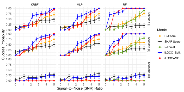
Figure A1: Success probability of detecting feature pair $(1,2)$ across SNR levels for KRBF, RF, and MLP regressors on nonlinear regression simulations (i), (ii), and (iii); the first feature pair has signal in scenarios (i) and (ii) whereas it is null in scenario (iii). Success probability is defined as the proportion of times the $(1,2)$ feature pair obtains the largest metric among all feature pairs. iLOCO-MP and iLOCO-Split consistently outperform existing approaches at detecting feature pair $(1,2)$ in the first two scenarios whereas iLOCO-MP exhibits superior specificity in the null scenario (iii).

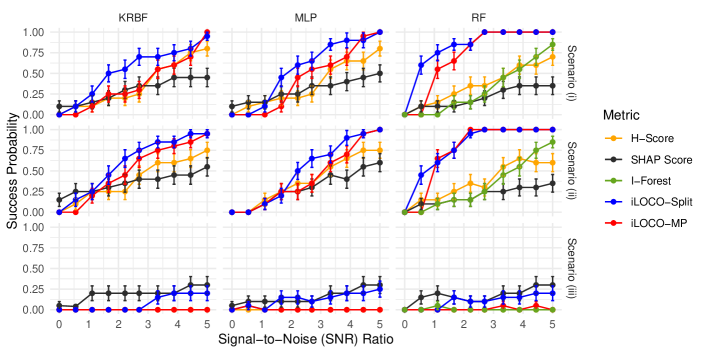
Figure A2: Success probability of detecting feature pair $(1,2)$ across SNR levels for KRBF, RF, and MLP classifiers on linear classification simulations (i), (ii), and (iii).

In the correlated simulations, shown in Figure A4, we evaluate our method on simulation (i), but we use an autoregressive design with $\boldsymbol{\Sigma}^{-1}_{j,j+1}=0.9$ instead of $\boldsymbol{\Sigma}=\mathbf{I}$ as in the uncorrelated $M$ simulations.

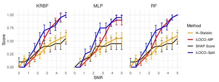
Figure A4: Success probability of detecting feature pair $(1,2)$ across SNR levels for KRBF, RF, and MLP regressors on the correlated simulation.

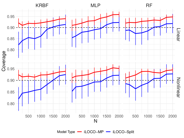
Figure A5: Coverage of 90% confidence intervals for $snr=2$ feature pair in synthetic regression simulation (i) using KRBF, MLP, and RF as the base estimators. iLOCO-MP exhibits slight over-coverage whereas iLOCO-Split has valid coverage greater 0.9 for sufficiently large sample size; this validates of inferential theory.

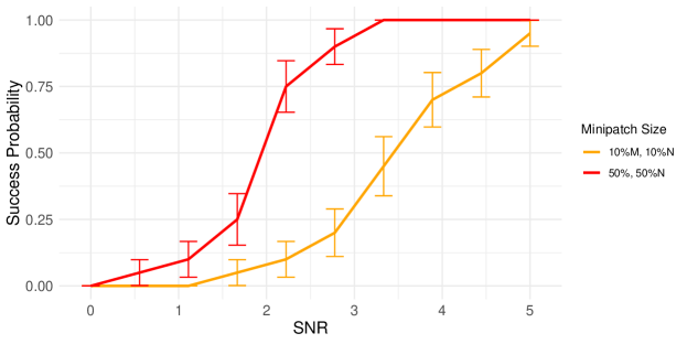
Figure A6: Comparison of minipatch sizes for KRBF regressor on simulation (i). iLOCO-MP detects feature pair (0,1) sooner when $m=50\%M$ and $n=50\%N$ than when $m=10\%M$ and $n=10N\%$, but the smaller minipatch size still consistently detects the feature pair when SNR = 5. This highlights the tradeoff between computational efficiency and accuracy and validates our use of $m=20\%M$ and $n=20\%N$ in our simulations.

Figure A7: iLOCO-MP metric for KRBF, RF, and MLP regressors evaluated on simulation (i).

References

- [1] Moloud Abdar, Farhad Pourpanah, Sadiq Hussain, Dana Rezazadegan, Li Liu, Mohammad Ghavamzadeh, Paul Fieguth, Xiaochun Cao, Abbas Khosravi and U Rajendra Acharya “A review of uncertainty quantification in deep learning: Techniques, applications and challenges” In Information fusion 76 Elsevier, 2021, pp. 243–297
- [2] André Altmann, Laura Toloşi, Oliver Sander and Thomas Lengauer “Permutation importance: a corrected feature importance measure” In Bioinformatics 26.10 Oxford University Press, 2010, pp. 1340–1347
- [3] Sven Apel, Sergiy Kolesnikov, Norbert Siegmund, Christian Kästner and Brady Garvin “Exploring feature interactions in the wild: the new feature-interaction challenge” In Proceedings of the 5th international workshop on feature-oriented software development, 2013, pp. 1–8
- [4] Sumanta Basu, Karl Kumbier, James B. Brown and Bin Yu “Iterative random forests to discover predictive and stable high-order interactions” In Proceedings of the National Academy of Sciences 115.8, 2018, pp. 1943–1948 DOI: 10.1073/pnas.1711236115
- [5] Yoav Benjamini and Daniel Yekutieli “False discovery rate–adjusted multiple confidence intervals for selected parameters” In Journal of the American Statistical Association 100.469 Taylor & Francis, 2005, pp. 71–81
- [6] Marko Bohanec “Car Evaluation” DOI: https://doi.org/10.24432/C5JP48, UCI Machine Learning Repository, 1988
- [7] Diffords “Difford’s Guide for Discerning Drinkers”, 2025 URL: https://www.diffordsguide.com/cocktails
- [8] Mengnan Du, Ninghao Liu and Xia Hu “Techniques for interpretable machine learning” In Communications of the ACM 63.1 ACM New York, NY, USA, 2019, pp. 68–77
- [9] Jerome H. Friedman and Bogdan E. Popescu “Predictive learning via rule ensembles” In The Annals of Applied Statistics 2.3 Institute of Mathematical Statistics, 2008 DOI: 10.1214/07-aoas148
- [10] Luqin Gan, Lili Zheng and Genevera I. Allen “Inference for Interpretable Machine Learning: Fast, Model-Agnostic Confidence Intervals for Feature Importance” arXiv, 2022 DOI: 10.48550/ARXIV.2206.02088
- [11] Ulrike Grömping “Variable importance assessment in regression: linear regression versus random forest” In The American Statistician 63.4 Taylor & Francis, 2009, pp. 308–319
- [12] Giles Hooker “Generalized functional anova diagnostics for high-dimensional functions of dependent variables” In Journal of computational and graphical statistics 16.3 Taylor & Francis, 2007, pp. 709–732
- [13] Roman Hornung and Anne-Laure Boulesteix “Interaction forests: Identifying and exploiting interpretable quantitative and qualitative interaction effects” In Computational Statistics and Data Analysis 171, 2022, pp. 107460 DOI: https://doi.org/10.1016/j.csda.2022.107460
- [14] Alan Inglis, Andrew Parnell and Catherine B. Hurley “Visualizing Variable Importance and Variable Interaction Effects in Machine Learning Models” In Journal of Computational and Graphical Statistics 31.3 TaylorFrancis, 2022, pp. 766–778 DOI: 10.1080/10618600.2021.2007935
- [15] Byol Kim and Rina Foygel Barber “Black-box tests for algorithmic stability” In Information and Inference: A Journal of the IMA 12.4 Oxford University Press, 2023, pp. 2690–2719
- [16] Jing Lei, Max G’Sell, Alessandro Rinaldo, Ryan J Tibshirani and Larry Wasserman “Distribution-free predictive inference for regression” In Journal of the American Statistical Association 113.523 Taylor & Francis, 2018, pp. 1094–1111
- [17] Jing Lei and Larry Wasserman “Distribution-free prediction bands for non-parametric regression” In Journal of the Royal Statistical Society Series B: Statistical Methodology 76.1 Oxford University Press, 2014, pp. 71–96
- [18] Jing Lei and Larry Wasserman “Distribution-free prediction bands for nonparametric regression” In Quality control and applied statistics 60.1 Executive Sciences Institute, 2015, pp. 109–110
- [19] Benjamin Lengerich, Sarah Tan, Chun-Hao Chang, Giles Hooker and Rich Caruana “Purifying interaction effects with the functional anova: An efficient algorithm for recovering identifiable additive models” In International Conference on Artificial Intelligence and Statistics, 2020, pp. 2402–2412 PMLR
- [20] Stan Lipovetsky and Michael Conklin “Analysis of regression in game theory approach” In Applied stochastic models in business and industry 17.4 Wiley Online Library, 2001, pp. 319–330
- [21] W James Murdoch, Chandan Singh, Karl Kumbier, Reza Abbasi-Asl and Bin Yu “Definitions, methods, and applications in interpretable machine learning” In Proceedings of the National Academy of Sciences 116.44 National Acad Sciences, 2019, pp. 22071–22080
- [22] Davide Napolitano, Lorenzo Vaiani and Luca Cagliero “Learning Confidence Intervals for Feature Importance: A Fast Shapley-based Approach.” In EDBT/ICDT Workshops, 2023
- [23] Giovanni Rabitti and Emanuele Borgonovo “A Shapley–Owen Index for Interaction Quantification” In SIAM/ASA Journal on Uncertainty Quantification 7.3, 2019, pp. 1060–1075 DOI: 10.1137/18M1221801
- [24] Marco Tulio Ribeiro, Sameer Singh and Carlos Guestrin “" Why should i trust you?" Explaining the predictions of any classifier” In Proceedings of the 22nd ACM SIGKDD international conference on knowledge discovery and data mining, 2016, pp. 1135–1144
- [25] Kanica Sachdev and Manoj Kumar Gupta “A comprehensive review of feature based methods for drug target interaction prediction” In Journal of biomedical informatics 93 Elsevier, 2019, pp. 103159
- [26] Wojciech Samek, Grégoire Montavon, Sebastian Lapuschkin, Christopher J Anders and Klaus-Robert Müller “Explaining deep neural networks and beyond: A review of methods and applications” In Proceedings of the IEEE 109.3 IEEE, 2021, pp. 247–278
- [27] Mukund Sundararajan, Kedar Dhamdhere and Ashish Agarwal “The Shapley Taylor Interaction Index” In Proceedings of the 37th International Conference on Machine Learning 119, Proceedings of Machine Learning Research PMLR, 2020, pp. 9259–9268 URL: https://proceedings.mlr.press/v119/sundararajan20a.html
- [28] Che-Ping Tsai, Chih-Kuan Yeh and Pradeep Ravikumar “Faith-Shap: The Faithful Shapley Interaction Index” In Journal of Machine Learning Research 24.94, 2023, pp. 1–42 URL: http://jmlr.org/papers/v24/22-0202.html
- [29] Isabella Verdinelli and Larry Wasserman “Decorrelated variable importance” In Journal of Machine Learning Research 25.7, 2024, pp. 1–27
- [30] Brian Williamson and Jean Feng “Efficient nonparametric statistical inference on population feature importance using Shapley values” In International conference on machine learning, 2020, pp. 10282–10291 PMLR
- [31] Brian D Williamson, Peter B Gilbert, Noah R Simon and Marco Carone “A general framework for inference on algorithm-agnostic variable importance” In Journal of the American Statistical Association 118.543 Taylor & Francis, 2023, pp. 1645–1658
- [32] Tianyi Yao and Genevera I Allen “Feature selection for huge data via minipatch learning” In arXiv preprint arXiv:2010.08529, 2020
- [33] Xiaoge Zhang, Felix TS Chan and Sankaran Mahadevan “Explainable machine learning in image classification models: An uncertainty quantification perspective” In Knowledge-Based Systems 243 Elsevier, 2022, pp. 108418
- [34] Pierre Bayle, Alexandre Bayle, Lucas Janson and Lester Mackey “Cross-validation Confidence Intervals for Test Error” In Advances in Neural Information Processing Systems 33 Curran Associates, Inc., 2020, pp. 16339–16350 URL: https://proceedings.neurips.cc/paper_files/paper/2020/file/bce9abf229ffd7e570818476ee5d7dde-Paper.pdf
- [35] Luqin Gan, Lili Zheng and Genevera I. Allen “Inference for Interpretable Machine Learning: Fast, Model-Agnostic Confidence Intervals for Feature Importance” arXiv, 2022 DOI: 10.48550/ARXIV.2206.02088
- [36] Alessandro Rinaldo, Larry Wasserman and Max G’Sell “Bootstrapping and sample splitting for high-dimensional, assumption-lean inference” In The Annals of Statistics 47.6 Institute of Mathematical Statistics, 2019, pp. 3438–3469 DOI: 10.1214/18-AOS1784