Generating Samples to Question Trained Models

Abstract

There is a growing need for investigating how machine learning models operate. With this work, we aim to understand trained machine learning models by questioning their data preferences. We propose a mathematical framework that allows us to probe trained models and identify their preferred samples in various scenarios including prediction-risky, parameter-sensitive, or model-contrastive samples. To showcase our framework, we pose these queries to a range of models trained on a range of classification and regression tasks, and receive answers in the form of generated data.

font=itshape, raggedright, noindent, leftmargin=0.15in, rightmargin=0.1in, begintext=“ , endtext= ”

1 Introduction

Machine learning models are widely used in today’s data-driven world, powering critical decision-making processes in sectors ranging from healthcare to human resources. Their widespread adoption in high-stakes scenarios raises important questions on aligning trained models with human values. Understanding how these models operate has become a critical aspect of addressing these concerns. Our quest along this line starts with the following inquiry: “What kind of data can we generate to probe our trained models?” We aim to study the implicit data distribution favored by trained models, illuminating potential tendencies and paving the way for more adaptable transparent systems.

To this end, we use an inductive approach to understand the model by creating samples in the data domain that the trained model considers favorable for a specific task. Traditional Machine Learning (ML) workflows emphasize data collection, cleaning, and model training. However, real-world applications present challenges such as ensuring alignment with human values and addressing issues in generating realistic representative data. For instance, a social benefit approval model may unfairly reject applications from underrepresented demographic groups (de Rechtspraak, 2020). Similarly, changes in data distributions over time can lead to model obsolescence, impacting predictions in critical areas like public health. Incorporating data generation that reveals the model’s preferences to the ML workflow can help mitigate these issues, enabling early warning systems and augmenting datasets to improve robustness.

Our goal is to understand models by generating data samples that are easy to interpret and showcase how the model answers specific questions posed to the model, rather than relying on feature saliency (Shrikumar et al., 2017) or surrogate model properties (Ribeiro et al., 2016) to explain an individual prediction. These questions are customized to each situation and can be expressed mathematically through a loss function that evaluates the data based on a combination of data characteristics and model parameters. We consider the problem of understanding a model to be a more nuanced endeavor that requires exploration across multiple dimensions of questioning. This involves providing explanations, such as counterfactual (Wachter et al., 2017) or prototypical (Biehl et al., 2016) scenarios, shedding light not only on why a particular prediction was made, but going beyond it as well. For instance, insights into model behavior can be gained by generating parameter-sensitive data samples or contrasting competing models through differentiating data. These custom questions, and others, provide a qualitative understanding of the model. Additionally, users have the flexibility to ask custom queries by designing specific probing functions within the data space.

Related Literature.

Our work complements extensive research in synthetic data generation. Synthetic data has been pivotal in addressing fairness, bias reduction, and robustness challenges in machine learning. Prior works have explored detecting bias in datasets (Kusner et al., 2017), using de-biased synthetic data to mitigate biased outputs (Xu et al., 2018; van Breugel et al., 2021), and employing synthetic data for dataset augmentation (Wong et al., 2016; Fawaz et al., 2018). Generative Adversarial Networks (GANs) and Variational Autoencoders (VAEs) have been widely used to approximate original data distributions (Goodfellow et al., 2014; Xu et al., 2018; Kingma & Welling, 2014; Breugel et al., 2024), focusing on privacy, diversity, and fidelity as primary goals.

Recent studies leveraged generative models for counterfactual generation and exploring underrepresented data regions. For example, Joshi et al. (2019) proposed a framework for generating task-specific synthetic data, enhancing model explainability. Similarly, Redelmeier et al. (2024) introduced an approach using autoregressive generative models to create counterfactuals, facilitating bias exploration and decision boundary analysis.

Energy-based models (EBMs) have also emerged as a promising framework, combining generative and discriminative modeling tasks. By treating classifier logits as an energy function, EBMs can model joint distributions over data and labels (LeCun et al., 2006; Duvenaud et al., 2020). Applications of EBMs include adversarial robustness, out-of-distribution detection, and data augmentation (Zhao et al., 2017; Liu et al., 2020; Arbel et al., 2021; Margeloiu et al., 2024). For instance, Duvenaud et al. (2020) demonstrated improved out-of-distribution detection using a joint energy-based model, while Ma et al. (2024) extended EBMs to tabular data for synthetic data generation.

The proposed framework draws inspiration from these works while introducing a distinct perspective. Our probing function can be seen as an energy function and leads to Gibbs distribution. However, rather than learning the energy function to capture the data distribution (conditioned on class), we create a probing function using trained models. This design allows the distribution to generate samples that address the specific posed question. Related works, such as (Duvenaud et al., 2020) and (Ma et al., 2024) mentioned above, adopt a similar approach by utilizing a trained classifier to obtain an energy function and using Langevin dynamics for sampling from the Gibbs distribution. However, their main objective is to mimic the true data distribution. In fact, the former paper combines training of the energy function and classifier. In contrast, we propose a flexible framework that allows for directing diverse queries to trained models via probing functions that reflect various objectives, such as identifying prediction-risky, parameter-sensitive, or model-contrastive data samples.

Contributions. We contribute to the literature by introducing a novel inductive approach. This approach creates data samples using a probing function that engages a trained model. Through this framework, the generated samples provide answers to various questions posed to trained models. With our computational study, we support our approach by applying it to a range of classification and regression tasks, showcasing its effectiveness in generating data tailored to specific queries. Our numerical results showcase the flexibility of our approach in uncovering biases, facilitating model interpretability, and consequently, promoting alignment of model predictions and human preferences.

2 The Mathematical Framework

Before we introduce the proposed framework, let us give our notation. The labeled data lie in $\mathcal{X}\times\mathcal{Y}$, and the model defines a predictor function $f({\boldsymbol{\mathbf{\theta}}},\cdot):\mathcal{X}\to\mathcal{Y}^{\prime}$ for any given set of model parameters ${\boldsymbol{\mathbf{\theta}}}\in\Theta$. Then, we obtain for a given sample ${\boldsymbol{\mathbf{x}}}\in\mathcal{X}$, the predicted label $y_{{\boldsymbol{\mathbf{\theta}}}}({\boldsymbol{\mathbf{x}}})\in\mathcal{Y}$ by passing the predictor function through a transformation depending on regression or classification task. The cost function $\ell_{F}:\mathcal{Y}\times\mathcal{Y}\to\mathbb{R}_{\geq 0}$ measures how far the predicted labels are from the true labels.

We propose a framework for probing a model with answers in the form of generated data. Our method is structured to be symmetric to the training process itself: instead of generating parameters given a data distribution, we generate data given a trained model parameter distribution, which may be a single set of parameters, i.e., a Dirac delta distribution. One can gain valuable insights into the trained model’s behavior by analyzing the generated population statistically. Figure 1 presents the overview of our framework.

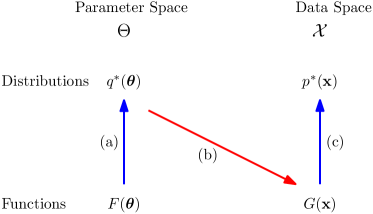
Figure 1: Overview of model probing by data generation. The vertical blue arrows (a) and (c) start from loss functions and lead to distributions on the same space by solving the Bayesian learning problem, which balances minimizing the expected loss with maximizing the entropy. The diagonal red arrow (b) obtains a loss function on the data space by integrating out the ${\boldsymbol{\mathbf{\theta}}}$ dependence from a designed function via $q^{*}({\boldsymbol{\mathbf{\theta}}})$. Samples following $p^{*}({\boldsymbol{\mathbf{x}}})$ constitute an answer to the question posed by $G$.

The standard construction of the parameter loss function is

$$F({\boldsymbol{\mathbf{\theta}}}) =\int_{\mathcal{X}\times\mathcal{Y}}(\ell_{F}(y_{\boldsymbol{\theta}}(\mathbf{x},y)+R_{F}(\boldsymbol{\theta}))\mathrm{d}\nu(\mathbf{x},y)$$

$$=\frac{1}{N}\sum_{i=1}^{N}\ell_{F}(y_{{\boldsymbol{\mathbf{\theta}}}}({\boldsymbol{\mathbf{x}}}_{i}),y_{i})+R_{F}({\boldsymbol{\mathbf{\theta}}}),$$

which can be seen as an integration of the function $\ell_{F}+R_{F}$ above against the empirical distribution given by the training dataset $\{({\boldsymbol{\mathbf{x}}}_{i},y_{i})\}_{i=1}^{N}\subseteq\mathcal{X}\times\mathcal{Y}$. Here, $R_{F}({\boldsymbol{\mathbf{\theta}}})$ is a regularizer term that depends only on ${\boldsymbol{\mathbf{\theta}}}$.

Similarly, we form a loss function $G$ on the data space by integrating out the ${\boldsymbol{\mathbf{\theta}}}$ dependence of a function of our design that depends both on the data and the model parameters. Depending on our choice, we end up probing the model with different questions. In Figure 1, the endpoint of the red arrow (b) is the function $G$, which is a mathematical model of the question posed to $q^{*}({\boldsymbol{\mathbf{\theta}}})$ at the tail of the arrow. A general form of such $G$ functions is given in (3) below.

The blue arrows (a) and (c) in Figure 1 represent solving the variational learning problem, which -instead of finding a single set of model parameters that minimizes a loss function- seeks for a distribution that balances the tasks of minimizing the expected loss and maximizing the entropy. In case of (a), we solve

$$\operatorname*{\arg\,\min}_{q\in\mathcal{Q}}\mathbb{E}_{q}[F]-\tau\mathcal{H}(q),$$ (1)

where $\mathcal{Q}$ is a choice of candidate distributions on $\Theta$, and $\mathcal{H}(q)=-\int_{\Theta}q\log q$ is the entropy with respect to a basis measure. The problem can be interpreted as an implementation of the exploration-exploitation trade-off in the parameter space. The constant $\tau>0$, called the temperature, controls the balance between these two objectives. Absent any restriction, i.e., if $\mathcal{Q}$ is the set of all probability distributions, then the Gibbs-Boltzmann distribution $q^{*}({\boldsymbol{\mathbf{\theta}}})\propto e^{-\frac{1}{\tau}F({\boldsymbol{\mathbf{\theta}}})}$ is the unique solution to (1).

Additionally, we point out that the well-known stochastic gradient descent training is not a significant departure from this setup, and in fact, can be seen as a specialization. Given a very restrictive family $\mathcal{Q}$, such as the manifold of Dirac delta distributions supported on a single ${\boldsymbol{\mathbf{\theta}}}$, the entropy term becomes irrelevant, and we get the classical optimization problem of minimizing the loss function $F$.

Completely symmetrically on the data space $\mathcal{X}$, the blue arrow denoted by (c) in Figure 1, represents solving the variational learning objective associated with the function $G$ on the data space

$$\operatorname*{\arg\,\min}_{p\in\mathcal{P}}\mathbb{E}_{p}[G]-\tau\mathcal{H}(p).$$ (2)

The expectation term encourages the solution $p^{*}({\boldsymbol{\mathbf{x}}})$ to concentrate its mass in regions where $G$ is minimized, but the entropy term encourages $p^{*}({\boldsymbol{\mathbf{x}}})$ to explore a wide variety of data samples. Here, $\mathcal{P}$ represents the family of candidate distributions, which can be chosen in several ways. One option is to explicitly select $\mathcal{P}$ as a family of distributions depending on the nature of the data distribution. Finally, we consider samples from the distribution $p^{*}({\boldsymbol{\mathbf{x}}})$ as answers to the questions put forth by $G$.

Alternatively, we can retain the full space of probability distributions but replace $G$ with $G\circ\varphi$ for some function $\varphi:\mathcal{Z}\to\mathcal{X}\times\mathcal{Y}$. In the latter case, $\mathcal{Z}$ can be the latent space and $\varphi$ can be the decoder function of a trained variational autoencoder. This procedure produces a distribution on $\mathcal{Z}$, which we can sample from and map to $\mathcal{X}$ via $\varphi$; thus, sampling data from the pushforward distribution. As a more mundane example, we may choose $\mathcal{Z}=\mathcal{X}$ with $\varphi({\boldsymbol{\mathbf{x}}})=({\boldsymbol{\mathbf{x}}},y^{\prime})$ for a fixed label $y^{\prime}$. If certain features of the data are considered immutable, then $\mathcal{Z}$ can be a certain subspace of $\mathcal{X}$ and $\varphi$ can be taken to map the missing features to predetermined fixed values. Alternatively, the label coordinate of $\varphi$ may also depend on ${\boldsymbol{\mathbf{x}}}$ using a classifier. We provide such examples in Section 3 and state precisely the questions posed to the model. As a last example of $\varphi$, if the data has been standardized to $[0,1]$, taking it to be the sigmoid function ensures that the answers to our questions come as data points with features in the admissible range.

We illustrate our framework with an explicit case. Consider a trained Linear Regression (LR) model. We probe this model by asking “What kind of data is truly preferred by the model for a fixed output value?” To model this question, the functions $\ell_{F}$ and $\ell_{G}$ are chosen as the squared difference. In this case, each step in Figure 1 can be solved analytically and the solutions are provided in Figure 2. The resulting preferred data distribution follows a normal distribution, where the formulas and the derivations for the mean $\widehat{{\boldsymbol{\mathbf{f}}}}$ and covariance matrix $\Sigma$ are given explicitly in Appendix A. In the next section, we dive into other probing questions and elaborate on their implications.

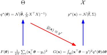
Figure 2: The proposed framework applied to a linear regression model with mean square error and no regularizers. Here, $y^{\prime}$ is a fixed output value. The distribution of data points ${\boldsymbol{\mathbf{x}}}$ which are preferred by the LR model for the prediction $y^{\prime}$ is calculated to be a Gaussian distribution centered at a point which is shifted from the mean of given data by a certain amount depending on the desired output value $y^{\prime}$. Details and derivation can be seen in Appendix A.

3 Probing Trained Models

We start with a general structure of the loss function that will be used for questioning the trained models:

$$G({\boldsymbol{\mathbf{x}}})=\int_{\Theta}\ell_{G}(y_{{\boldsymbol{\mathbf{\theta}}}}({\boldsymbol{\mathbf{x}}}),\widehat{y}({\boldsymbol{\mathbf{x}}}))q^{*}({\boldsymbol{\mathbf{\theta}}})\mathrm{d}\,{\boldsymbol{\mathbf{\theta}}}+R_{G}({\boldsymbol{\mathbf{x}}}),$$ (3)

where $\widehat{y}$ stands for a predictor and $R_{G}$ is a regularizer function that can be chosen to put additional soft constraints on the samples in addition to the hard constraints coming from the restriction $p\in\mathcal{P}$. To question the models, we next consider various scenarios with different loss functions, which are the special cases of the general structure in (3).

Fixed-label samples.

We probe the model for what it thinks are good data samples from the distribution $\mathcal{P}$ that fit the bill for $\widehat{y}({\boldsymbol{\mathbf{x}}})\equiv y^{\prime}$. This can be applied to a single set of model parameters ${\boldsymbol{\mathbf{\theta}}}^{*}$, or to a general ensemble of models where the parameters are coming from a distribution $q^{*}({\boldsymbol{\mathbf{\theta}}})$.

In case of a single set of problem parameters, we obtain

$$G({\boldsymbol{\mathbf{x}}})=\ell_{G}(y_{{\boldsymbol{\mathbf{\theta}}}^{*}}({\boldsymbol{\mathbf{x}}}),y^{\prime})+R_{G}({\boldsymbol{\mathbf{x}}}).$$ (4)

When parameters are coming from a distribution, the loss function becomes

$$G({\boldsymbol{\mathbf{x}}})=\int_{\Theta}\ell_{G}(y_{{\boldsymbol{\mathbf{\theta}}}}({\boldsymbol{\mathbf{x}}}),y^{\prime})q^{*}({\boldsymbol{\mathbf{\theta}}})\mathrm{d}\,{\boldsymbol{\mathbf{\theta}}}+R_{G}({\boldsymbol{\mathbf{x}}}).$$ (5)

Figure 2 demonstrates the steps when $y_{{\boldsymbol{\mathbf{\theta}}}}({\boldsymbol{\mathbf{x}}})={\boldsymbol{\mathbf{x}}}^{\intercal}{\boldsymbol{\mathbf{\theta}}}$ corresponds to linear regression, and both $\ell_{F}$ and $\ell_{G}$ are the mean squared errors. Recall for this special case that we obtain analytical solutions for all steps of our framework. The details of this observation are given in Appendix A.

Prediction-risky samples.

Suppose that a model predicts probabilities such as in logistic regression and the logit layers of neural networks before thresholding. Assuming the predictions correspond directly to these probabilities, that is, $y_{{\boldsymbol{\mathbf{\theta}}}}(\mbox{\boldmath{$x$}})=f(\mbox{\boldmath{$x$}},{\boldsymbol{\mathbf{\theta}}})$, and $\widehat{y}({\boldsymbol{\mathbf{x}}})\equiv{\boldsymbol{\mathbf{\alpha}}}$ for some anchor probability value, we can probe the model by evaluating the probability spread using $r$-norm, i.e., $\ell_{G}(y,y^{\prime})=\|y-y^{\prime}\|_{r}$ for $r\geq 1$. We then seek data points with probabilities close to ${\boldsymbol{\mathbf{\alpha}}}$. For a binary classification with the anchor value $0.5$, this corresponds to generating “risky data points” near the decision boundary.

Parameter-sensitive samples.

Given a set of parameters ${\boldsymbol{\mathbf{\theta}}}^{*}$ and the distribution $q^{*}({\boldsymbol{\mathbf{\theta}}})$, we ask the model for data samples that are classified as one value, but would be classified as another if the model parameters were to (perhaps slightly) be perturbed. That is

$$G({\boldsymbol{\mathbf{x}}})=\int_{\Theta}\ell_{G}(y_{{\boldsymbol{\mathbf{\theta}}}}({\boldsymbol{\mathbf{x}}}),1-y_{{\boldsymbol{\mathbf{\theta}}}^{*}}({\boldsymbol{\mathbf{x}}}))q^{*}({\boldsymbol{\mathbf{\theta}}})\mathrm{d}\,{\boldsymbol{\mathbf{\theta}}}+R_{G}({\boldsymbol{\mathbf{x}}}),$$ (6)

where we take $\widehat{y}({\boldsymbol{\mathbf{x}}})\equiv 1-y_{\theta^{*}}({\boldsymbol{\mathbf{x}}})$ denoting the flipped classification decision that contrasts the model’s decision with a fixed set of parameters, ${\boldsymbol{\mathbf{\theta}}}^{*}$. When $\mathcal{Q}$ is a restricted to a family of distributions, like Gaussians with fixed variance, sampling from $q^{*}({\boldsymbol{\mathbf{\theta}}})$ corresponds to sampling from the vicinity of ${\boldsymbol{\mathbf{\theta}}}^{*}$.

There is a notable distinction between prediction-risky and parameter-sensitive samples. Prediction-risky samples tend to be generated near the decision boundary, while parameter-sensitive case has the flexibility to generate samples that can be near or far from the decision boundary. We further elaborate on this distinction in our computational study section.

Model-contrasting samples.

We note that the predictor $\widehat{y}$ does not necessarily have to be derived from the current model. It can also be obtained from a different model that we are comparing our current model against. With the function

$$G({\boldsymbol{\mathbf{x}}})=\ell_{G}(y_{{\boldsymbol{\mathbf{\theta^{*}}}}}({\boldsymbol{\mathbf{x}}}),1-\widehat{y}({\boldsymbol{\mathbf{x}}}))+R_{G}({\boldsymbol{\mathbf{x}}}),$$ (7)

we are asking where our (e.g., linear regression) model differs from another (e.g., XGBoost) model.

Localized samples.

In all of the above cases, we can add a regularizer term $R_{G}({\boldsymbol{\mathbf{x}}})=\|{\boldsymbol{\mathbf{x}}}-{\boldsymbol{\mathbf{x}}}_{s}\|_{r}$ for $r\geq 1$ to generate synthetic data that is similar locally to a given ${\boldsymbol{\mathbf{x}}}_{s}$. In fact, different weightings can also be applied to different columns to enforce this more or less stringently for different features.

Feature-restricted samples.

By restricting $\mathcal{P}$ to be supported on data with certain features fixed, such as those features corresponding to age, race, and so on, we can ask the model for all of the above questions but conditioning on certain immutable characteristics. This falls into the class of optimizations, where instead of $G$ we consider $G(\varphi(\mbox{\boldmath{$z$}}))$ on some other (latent) space $\mbox{\boldmath{$z$}}\in Z$. In case of image data, for example, to have our samples conform to the data manifold, $\varphi$ can be taken as the trained decoder module from a VAE. Then, starting with measures $\widetilde{p}\in\mathcal{P}(Z)$ on the latent space, their pushforwards $\varphi_{*}\widetilde{p}$ lie on the data manifold, i.e., sampling $\mbox{\boldmath{$z$}}\sim\widetilde{p}$ and computing $\varphi(\mbox{\boldmath{$z$}})$ gives a data sample.

4 Computational Study

In this section, we conduct a set of experiments to evaluate the cases presented in Section 3. Our experiments aim to evaluate the proposed framework by demonstrating its ability to generate data samples across various scenarios. We use well-known datasets from the literature, and their specifics are outlined in Appendix B. The implementation details and code for reproducing these experiments are available on our GitHub repository.

Fixed-label samples.

We apply the probing function $G$ in (5) to the Adult dataset (Becker & Kohavi, 1996) obtained from US census data that is widely used as a benchmark for the binary classification task with the binarized income column (giving whether the individual makes $>$$$50$k annually or not) as the response variable. We train a logistic regression model on this dataset and examine the behavior of this model by constructing counterfactual samples. Specifically, we choose a data sample $({\boldsymbol{\mathbf{x}}}_{0},y)$, and use the probing function (5) with $y^{\prime}\neq y$ and $R({\boldsymbol{\mathbf{x}}})=\|\mbox{\boldmath{$x$}}-\mbox{\boldmath{$x$}}_{0}\|^{2}$.

For this experiment, the factual instance represents an unmarried Latin-American Black Female, currently predicted to earn less than $50K. Through our framework, we pose the question:

What changes in the input features would lead to this individual being classified as having an income greater than $50K?

To address this question, the probing function is designed to generate counterfactual samples by balancing two key objectives: aligning the model’s predictions with the desired target label and maintaining proximity to the factual instance. The cost function $\ell_{G}(y_{{\boldsymbol{\mathbf{\theta}}}}({\boldsymbol{\mathbf{x}}}),y^{\prime})$ given in (5) is formulated based on the cross-entropy loss with $y^{\prime}=1$, and the regularizer term $R_{G}({\boldsymbol{\mathbf{x}}})$ penalizes large deviations between the counterfactual samples and the factual instance.

Figure 3 illustrates the distribution of the generated samples. The results provide insights into the model’s classification process and the factors it deems influential in income predictions. While generating counterfactual samples, we impose limitations (lower and upper bounds) on the potential values of certain features, namely age, educational attainment, and weekly working hours. These bounds are integrated into the Langevin dynamics sampling process, which ensures that each step is clipped to remain within the specified ranges. Additionally, we note that in all our experiments, the generated samples are projected to stay within the feature value ranges observed in the original dataset (i.e. the given training and test set). In Figure 3, the factual instance is marked in red, with a vertical dashed line for numerical features and a red text label for categorical features. A comparison between the factual instance and the distribution of counterfactual samples reveals significant categorical changes. For example, the majority of counterfactual samples indicate a change in gender from female to male, and the native country shifts from Latin America to Western Europe. Gender and native-country columns show implications for fairness and bias. Since we opted for logistic regression as our trained model, one may also directly investigate the coefficients associated with these features. However, the bias towards the male gender is more difficult to observe from the respective coefficients (female $\approx-1.375$ vs. male $\approx-1.243$) than from the generated data. More importantly, such coefficients are not readily available for more complex models like deep networks.

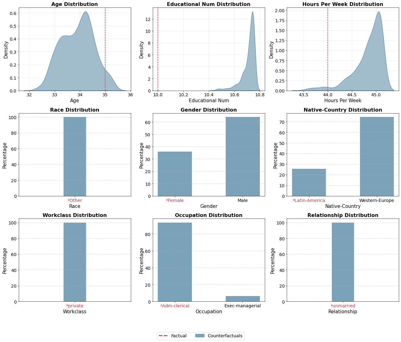
Figure 3: Feature distributions of generated counterfactual samples (blue shaded) with factual instance highlighted (red markers).

Prediction-risky samples.

This experiment aims to explore data samples near the decision boundary, where model predictions are inherently uncertain. To guide this analysis, we pose the following question to our framework: What kind of data samples are predicted to be risky due to being close to a specific anchor value? For this experiment, we use the FICO dataset (FICO, 2018), which consists of credit applications with features related to financial history and risk performance. A neural network (MLP) is trained to predict whether a customer belongs to the “Good” or “Bad” credit class. To identify boundary samples, we define the decision boundary as the region where the model’s predicted probabilities are close to the anchor value of 0.5. Using our framework, we generate and analyze 500 boundary samples to gain insights into the characteristics of individuals who are borderline cases for classification. The mean probability of belonging to the “Bad” credit class for these generated prediction-risky samples is calculated as 0.525, with a standard deviation of 0.017.

The density plots in Figure 4 compare the distributions of two representative features in the original data and the generated prediction-risky samples. The feature NumTrades60Ever2DerogPubRec represents the number of past credit trades, where payments were delayed by at least 60 days, serving as a key indicator of past delinquency. As shown in Figure 4(a), the distribution of risky samples follows the original data closely, particularly in the lower range. However, the generated samples exhibit a stronger peak around zero, indicating that the model considers individuals with few or no past delinquencies as borderline cases. This implies that, for individuals with little to no history of late payments, the model seems to find it more difficult to make a confident classification, likely due to a lack of strong negative or positive indicators. The feature MSinceOldestTradeOpen represents the number of months since a customer’s first credit line was opened, effectively capturing the length of their credit history. As seen in Figure 4(b), the distribution of generated risky samples is highly concentrated around 400 months ($\sim$33 years), whereas the original data is spread over a much wider range. This behavior suggests that the model associates longer credit histories with greater uncertainty in classification. The sharp peak around this value indicates that the model fixates on long-established credit histories as an ambiguous factor when making predictions. For additional comparison, the distributions of the remaining features can be found in Appendix C.

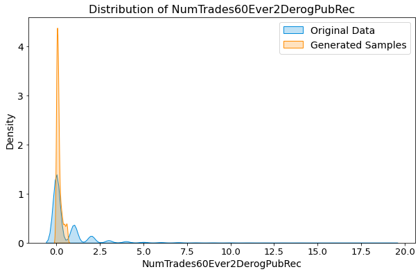
(a) Feature distribution in the original data.

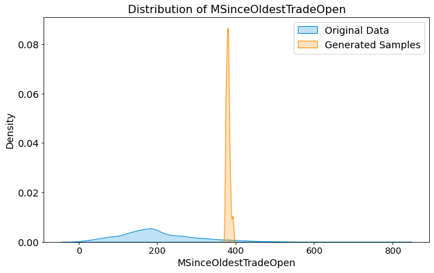
(b) Feature distribution in the generated samples.

Figure 4: Feature distributions in the original data and generated prediction-risky samples.

Parameter-sensitive samples.

This experiment investigates data samples that are sensitive to small perturbations in the model parameters. Unlike prediction-risky samples, which are concentrated near the decision boundary, parameter-sensitive samples may exist anywhere in the input space, as their classification changes when the model parameters shift slightly. To guide this analysis, we pose the following question to our framework: What kind of data samples would exhibit prediction instability under small perturbations of the model parameters?

For this experiment, we train an MLP model on the FICO dataset to identify parameter-sensitive samples and directly compare the findings with those obtained for prediction-risky samples. To generate parameter-sensitive samples, we perturb the model parameters by sampling from a Gaussian distribution centered at the original parameters with a fixed variance. Using the probing function in (6), we generate and analyze 500 samples to understand which instances are most susceptible to changes in model parameters.

The density plots in Figure 5 compare the distributions of four representative features (see Appendix C for the remaining features) in the generated parameter-sensitive samples and prediction-risky samples. By comparing these two distributions, we gain insights into how the model perceives uncertainty from different perspectives. While the prediction-risky samples are associated with uncertainty near the decision boundary, the parameter-sensitive samples highlight regions in the feature space where small perturbations in the model’s parameters can lead to classification shifts. The features AverageMinFile (average observation period) and NumTotalTrades (total number of trades) exhibit similar distributions across both generated sample types. In contrast, the features MSinceMostRecentTradeOpen (months since most recent trade opened) and NumInqLast6M (the number of inquiries in the last six months) show a clear divergence. For instance, NumInqLast6M represents the number of times a customer has had their credit history checked in the last six months, which is often linked to recent credit-seeking behavior. For this feature, the prediction-risky samples cluster around lower values, suggesting that individuals with fewer recent inquiries are more likely to be classified as borderline cases. On the other hand, the parameter-sensitive samples exhibit a broader and more spread-out distribution, indicating that parameter shifts affect individuals across a wider range of credit-scoring inquiries. This may be because frequent inquiries can indicate diverse financial behaviors, making these samples more susceptible to instability when model parameters change. These findings suggest that certain features contribute more significantly to classification robustness against parameter variations, whereas others primarily influence boundary-sensitive classifications.

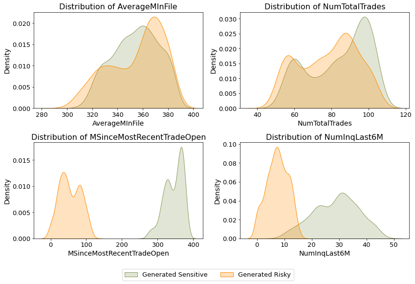
Figure 5: Feature distributions in generated parameter-sensitive and prediction-risky samples.

Model-contrasting samples.

This experiment investigates the differences between two predictive models by probing the features that drive contrasting predictions for the same data. Through our framework, we pose: Which specific features or input changes lead to disagreement between the two models’ predictions?

For this experiment, we use datasets that have two different modalities: tabular and visual. The tabular datasets include Housing (Kaggle, 2021) and FICO, while the visual dataset is MNIST (LeCun et al., 2010).

In the Housing dataset experiment, we compare support vector regression (SVR) and LR models. We split the dataset into training-test sets and trained both models on the same training data. To generate data samples where the two models diverge in their predictions, we formulate the cost function given in (7) as $\ell_{G}(y_{1},1-y_{2})=\exp(-(y_{1}-y_{2})^{2})$. Using our framework, we generate data samples to identify the regions of the input space where the models exhibit significant disagreement, likely due to their differing assumptions about feature interactions and predictive mechanisms.

Figure 6 presents a scatter plot comparing the predictions of the LR and SVR models. The blue points represent the predictions of the models in the test data, demonstrating that the two models generally produce highly similar outputs, with minimal differences observed. The green points, on the other hand, represent generated samples, highlighting instances where the models exhibit contrasting predictions. The zoomed-in inset further emphasizes these discrepant predictions, demonstrating that our framework effectively identifies and generates data points that maximize the divergence between the two models.

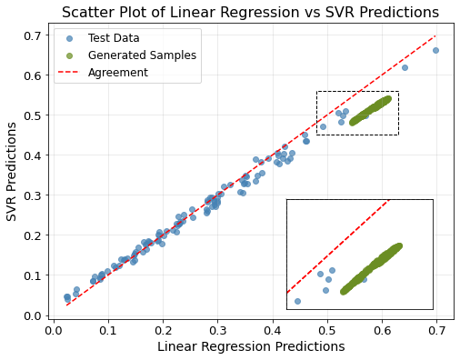
Figure 6: Comparison of SVR and LR predictions on test data and generated samples.

Figure 7 compares the feature distributions between the synthetic dataset generated by our framework and the test data. The box plots represent the range of values for each feature, with blue corresponding to the test data and green representing the generated samples. This figure provides a clear visualization of how the generated data differs from the test data in terms of feature distributions. For instance, as the number of bathrooms and stories increases, the model predictions diverge. Additionally, hot water heating and air conditioning exhibit a distinct concentration in the synthetic data, with most generated samples clustering around higher values compared to the test data. This suggests that these features play a prominent role in distinguishing instances where the models behave differently. Overall, this figure offers insights into how the generated samples differ from the original dataset, highlighting key feature distributions that drive divergence in model predictions and providing a deeper understanding of how our framework probes model behavior.

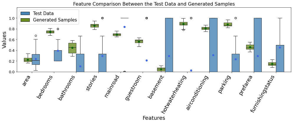
Figure 7: Feature distribution in test data and generated samples that produce different predictions for SVR and LR.

We can also investigate model divergence in cases where the comparison model is non-differentiable. To demonstrate this, we train XGBoost -a non-parametric model- alongside logistic regression on the FICO dataset. This setup highlights the flexibility of our framework, as it allows us to probe differences between fundamentally different modeling approaches. Two models agree on 94.5% of the predictions in the test data. However, we generate a set of samples where the models exhibit full disagreement, i.e., XGBoost predicts one class, while logistic regression predicts the opposite. Figure 8 presents the feature distributions for these discrepant samples, focusing on four representative features.

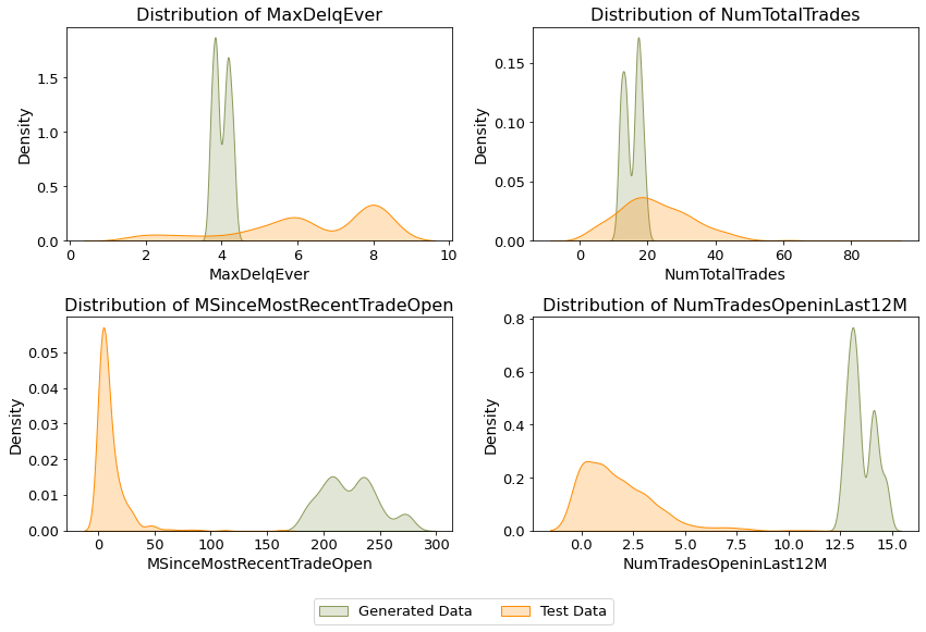
Figure 8: The distributions of four representative features in the generated samples. Here, XGBoost predicts “Bad” for RiskPerformance, while logistic regression predicts “Good”.

Our framework can also be used to compare and contrast two models trained on image data. To demonstrate, we consider a Convolutional Neural Network (CNN) and an MLP, both trained on MNIST. The architectural details of these networks are provided in Appendix B.2. To better capture the data manifold, we also train a VAE with a latent dimension of 10. The trained encoder module of the VAE is denoted by $z\mapsto\varphi(z)$. Further details on the VAE training process are provided in Appendix D. In Figure 9, we present an example computation illustrating how this setup works. Starting with a latent vector encoding an image with label ‘3’, we sample from a distribution that prefers the label ‘8’ jointly for both a trained CNN (LeNet5) and an MLP.

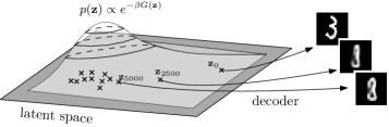
Figure 9: Using Langevin dynamics in the latent space, we obtain a sequence of latent vectors that, when passed through the decoder $\varphi$, correspond to a walk on the data manifold. In this image, the function $G$ is the sum of cross entropy predictions of trained MLP and LeNet5 networks for the label ‘8’ and for the data $\varphi(z)$.

We use this setup to systematically compare the CNN and MLP models. In Figure 10, we showcase some samples generated by forcing functions $G$ that pull the data in incompatible directions, for example resulting in amorphous data points that exhibit characteristics of both ‘1’ and ‘0’. The third column highlights cases where the label ‘8’ is preferred (top: MLP, bottom: CNN) while remaining close to an actual MNIST image labeled ‘3’, which is enforced through two-norm regularization.

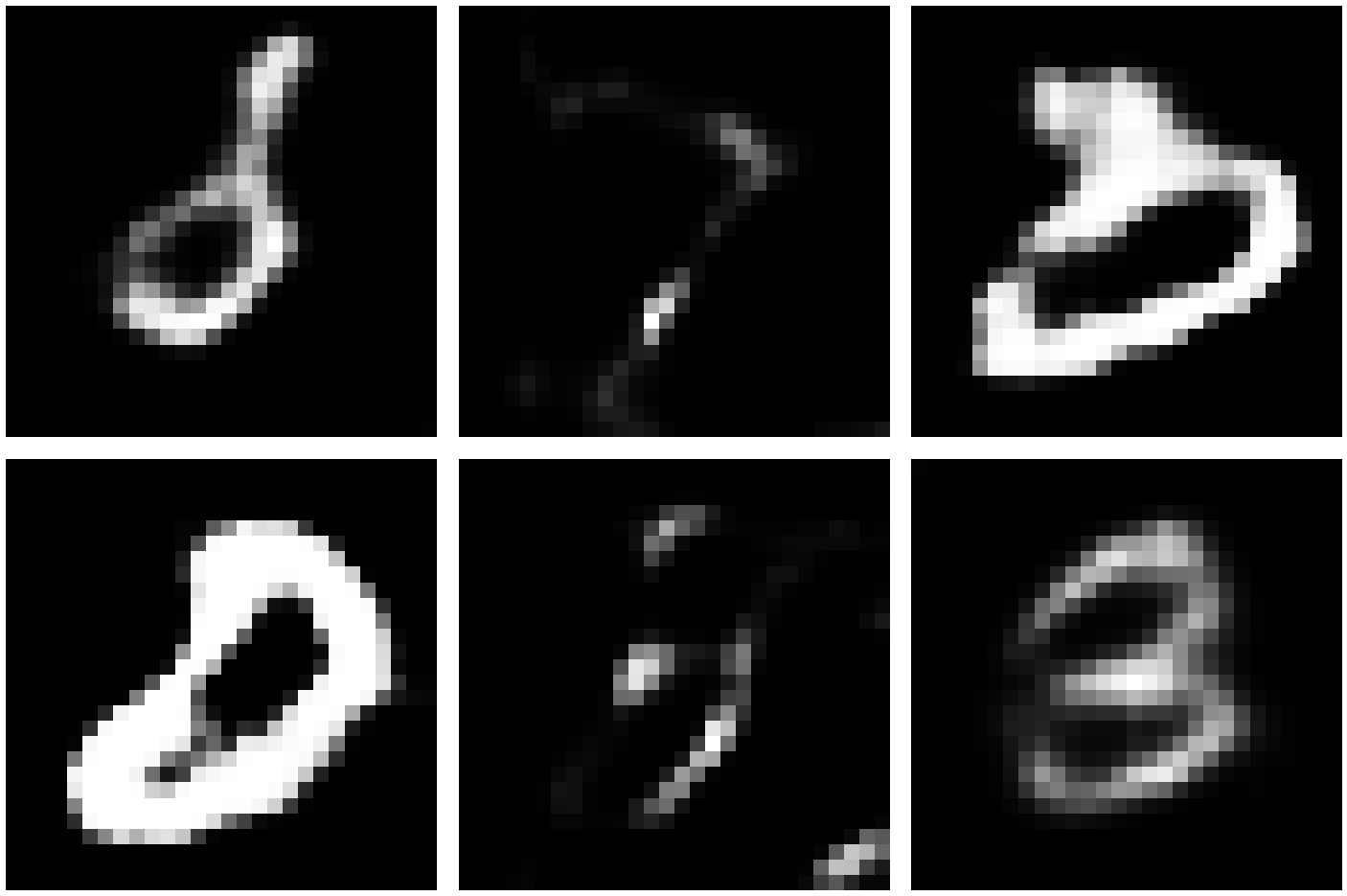
Figure 10: Images in the first and second columns are generated to prefer a given label on an MLP model and another one on a CNN model. upper-left: CNN-‘0’ MLP-‘1’, upper-middle: CNN-‘1’ MLP-‘7’, lower-left: CNN-‘0’ MLP-‘8’, lower-middle: CNN-‘2’ MLP-‘5’. On the third column, the upper image prefers the label ‘8’ for the MLP model whilst being close to a data sample with label ‘3’, and the same for the lower image for the CNN model.

5 Conclusion

In this work, we propose a mathematical framework for probing trained models by generating data samples tailored to specific queries. Our approach provides a novel way to understand model behavior beyond well-known interpretability methods, such as feature saliency or surrogate models. By formulating probing functions, we demonstrate how to generate samples under various scenarios such as prediction-risky, parameter-sensitivity, and contrasting models. Our computational study confirms the effectiveness of the proposed framework across classification and regression tasks on various datasets, providing insights into model decision boundaries and sensitivity to input perturbations.

Despite its strengths, our framework has certain limitations. First, scaling to larger models, particularly deep learning architectures with billions of parameters, poses computational challenges. The iterative optimization and sampling procedures may become prohibitively expensive in such settings. Furthermore, due to implicit constraints among the features, our method may generate samples that are not representative enough of the dataset, potentially leading to narrow conclusions.

For future research, an interesting direction is incorporating constraints among features to ensure that the generated samples remain plausible and adhere to known data dependencies. For instance, enforcing domain-specific relationships, such as monotonic constraints among features, could enhance the interpretability and reliability of the generated samples. By addressing these aspects, we can further refine data-driven explainability techniques.

Appendix A Linear Regression with Gaussian Data

We start with $y_{\boldsymbol{\theta}}(\mathbf{x})=\boldsymbol{\theta}^{\top}\mathbf{x}$ and $\ell_{F}(y,y^{\prime})=\ell_{G}(y,y^{\prime})=\frac{1}{2}(y-y^{\prime})^{2}$. Given a dataset $\{(\mathbf{x}_{i},y_{i})\}_{i=1}^{N}$, we construct the loss function $F({\boldsymbol{\theta}})$ as the integral of $\ell_{F}(y_{\boldsymbol{\theta}}(\mathbf{x}),y)$, over the data distribution, which is approximated by the Dirac delta comb $\nu=\frac{1}{N}\sum_{i=1}^{N}\delta_{(\mathbf{x}_{i},y_{i})}$:

$$F({\boldsymbol{\theta}})=\int_{\mathcal{X}\times\mathcal{Y}}\!\!\!\!\ell_{F}(y_{\boldsymbol{\theta}}(\mathbf{x}),y)\mathrm{d}\,\nu(\mathbf{x},y)=\frac{1}{2N}\sum_{i=1}^{N}|\mathbf{x}_{i}^{\top}{\boldsymbol{\theta}}-y_{i}|^{2}.$$

Assume, for convenience, that a constant feature of 1 is included as the last coordinate of $\mathbf{x}$, allowing us to explicitly represent the intercept. Using this notation, we define

$$\mathbf{x}=\begin{bmatrix}\mathbf{f}\\ 1\end{bmatrix},\qquad{\boldsymbol{\theta}}=\begin{bmatrix}{\boldsymbol{\xi}}&b\end{bmatrix},\text{ so that }\mathbf{x}^{\top}{\boldsymbol{\theta}}=\mathbf{f}^{\top}{\boldsymbol{\xi}}+b.$$

We write the design matrix as

$$D=\left[\begin{array}[]{ccc;{2pt/2pt}c}\cdots&\mathbf{x}_{1}^{\top}&\cdots&1\\ \cdots&\mathbf{x}_{2}^{\top}&\cdots&1\\ &\vdots&&\vdots\\ \cdots&\mathbf{x}_{N}^{\top}&\cdots&1\end{array}\right]=\left[\begin{array}[]{c;{2pt/2pt}c}X&\mathbf{1}\end{array}\right].$$

The quadratic loss function can then be expressed as

$$F({\boldsymbol{\theta}})=\frac{1}{2N}\|D{\boldsymbol{\theta}}-\mathbf{y}\|^{2},$$

where $\mathbf{y}=\begin{bmatrix}y_{1}&y_{2}&\cdots&y_{N}\end{bmatrix}^{\top}$ is the label vector. We can reorder the terms so that

$$F({\boldsymbol{\theta}}) =\frac{1}{2N}(D{\boldsymbol{\theta}}-y)^{\top}(D{\boldsymbol{\theta}}-y)=\frac{1}{2N}\left({\boldsymbol{\theta}}^{\top}D^{\top}D{\boldsymbol{\theta}}-2{\boldsymbol{\theta}}^{\top}X^{\top}\mathbf{y}\right)+\text{const.}$$

$$=\frac{1}{2}({\boldsymbol{\theta}}-\widehat{{\boldsymbol{\theta}}})^{\top}\frac{D^{\top}D}{N}({\boldsymbol{\theta}}-\widehat{{\boldsymbol{\theta}}})+\text{const}.$$

where $\widehat{{\boldsymbol{\theta}}}=(D^{\top}D)^{-1}D^{\top}\mathbf{y}$. Note that this is precisely the ordinary least squares solution.

Since the loss function is quadratic, we can explicitly write the Gibbs distribution (which is the unrestricted solution to the Bayesian Learning Problem with $F$) as the Gaussian distribution

$$q^{*}(\theta)\propto e^{-\beta F(\theta)}\propto e^{-\frac{1}{2}({\boldsymbol{\theta}}-\widehat{{\boldsymbol{\theta}}})^{\top}\frac{D^{\top}D}{N/\beta}({\boldsymbol{\theta}}-\widehat{{\boldsymbol{\theta}}})}\quad\text{thus }q^{*}(\mathbf{\theta})=\mathcal{N}\left(\widehat{{\boldsymbol{\theta}}},\left(\frac{D^{\top}D}{N/\beta}\right)^{-1}\right).$$

Here, the variable $\beta$ is the inverse temperature defined as $\beta=1/\tau$.

Next, we construct $G$, a loss function on $\mathcal{X}\times\mathcal{Y}$. By fixing the label, we may also consider $G$ as a loss function only on $\mathcal{X}$, from which we derive a distribution over $\mathcal{X}$. To avoid overusing $\mathbf{x}$ and $y$, we denote elements of the labeled dataset as $(\mathbf{z},w)\in\mathcal{X}\times\mathcal{Y}$ with $\mathbf{z}=\left[\begin{smallmatrix}\mathbf{f}\\ 1\end{smallmatrix}\right]$. Using the first and second moments of Gaussians, we calculate

$$G(\mathbf{z},w) =\int_{\Theta}|\mathbf{z}^{\top}{\boldsymbol{\theta}}-w|^{2}q^{*}({\boldsymbol{\theta}})\mathrm{d}\,\theta$$

$$=\mathbf{z}^{\top}\mathbb{E}_{q^{*}}[{\boldsymbol{\theta}}{\boldsymbol{\theta}}^{\top}]\mathbf{z}-2w\mathbf{z}^{\top}\mathbb{E}_{q^{*}}[{\boldsymbol{\theta}}]+\text{ const}$$

$$=\mathbf{z}^{\top}\left(\widehat{{\boldsymbol{\theta}}}\widehat{{\boldsymbol{\theta}}}^{\top}+\left(\frac{D^{\top}D}{N\tau}\right)^{-1}\right)\mathbf{z}-2w\mathbf{z}^{\top}\widehat{{\boldsymbol{\theta}}}+\text{ const}.$$

which is again a quadratic function in $\mathbf{z}.$ Let us now write this quadratic in terms of $\mathbf{f}$. We write $\widehat{{\boldsymbol{\theta}}}=\left[\begin{smallmatrix}\widehat{{\boldsymbol{\xi}}}\\ \widehat{b}\end{smallmatrix}\right]$.

First, a quick calculation gives the block diagonal form

$$\left(\frac{D^{\top}D}{N\tau}\right)^{-1} =\tau\left[\begin{array}[]{c;{3pt/3pt}c}\frac{X^{\top}X}{N}&\lx@text@overline{\mathbf{x}}\\ \hdashline[3pt/3pt]\overline{\mathbf{x}}^{\top}&1\end{array}\right]^{-1}$$

$$=\tau\left[\begin{array}[]{c;{3pt/3pt}c}A^{-1}&-A^{-1}\lx@text@overline{\mathbf{x}}\\ \hdashline[3pt/3pt]-\overline{\mathbf{x}}^{\top}A^{-1}&*\end{array}\right],$$

where $A=\frac{X^{\top}X}{N}-\overline{\mathbf{x}}\overline{\mathbf{x}}^{\top}$ is the Schur complement and $\overline{\mathbf{x}}=\frac{1}{N}\sum_{i=1}^{N}\mathbf{x}_{i}$ is the mean data vector.

We can write $G$ as a quadratic function of $\mathbf{f}$ (fixing $w$) as

$$G_{w}(\mathbf{f}) =\mathbf{f}^{\top}\left(\tau A^{-1}+\widehat{{\boldsymbol{\xi}}}\widehat{{\boldsymbol{\xi}}}^{\top}\right)\mathbf{f}-2\mathbf{f}^{\top}\left(\tau A^{-1}\overline{\mathbf{x}}-\widehat{{\boldsymbol{\xi}}}\hat{b}+w\hat{b}\right)+\text{const.}$$

$$=(\mathbf{f}-\widehat{\mathbf{f}})\left(\tau A^{-1}+\widehat{{\boldsymbol{\xi}}}\widehat{{\boldsymbol{\xi}}}^{\top}\right)(\mathbf{f}-\widehat{\mathbf{f}})+\text{const}.$$

Here, $\widehat{\mathbf{f}}$ is calculated as

$$\widehat{\mathbf{f}} =\left(\tau A^{-1}+\widehat{{\boldsymbol{\xi}}}\widehat{{\boldsymbol{\xi}}}^{\top}\right)^{-1}\left(\tau A^{-1}\overline{\mathbf{x}}+\widehat{{\boldsymbol{\xi}}}(w-\hat{b})\right)$$

$$=\left(A_{\tau}-\frac{A_{\tau}\widehat{{\boldsymbol{\xi}}}\widehat{{\boldsymbol{\xi}}}^{\top}A_{\tau}}{1+\widehat{{\boldsymbol{\xi}}}^{\top}A_{\tau}\widehat{{\boldsymbol{\xi}}}}\right)\left(A_{\tau}^{-1}\overline{\mathbf{x}}+\widehat{{\boldsymbol{\xi}}}^{\top}(w-\hat{b})\right),$$

where $A_{\tau}=\frac{1}{\tau}A$ and the Sherman-Morrison formula is used for inverting the matrix.

Now expanding the product, we obtain

$$\widehat{\mathbf{f}}=\overline{\mathbf{x}}+A_{\tau}\widehat{{\boldsymbol{\xi}}}(w-\hat{b})-\frac{A_{\tau}\widehat{{\boldsymbol{\xi}}}\widehat{{\boldsymbol{\xi}}}^{\top}\overline{\mathbf{x}}}{1+\widehat{{\boldsymbol{\xi}}}^{\top}A_{\tau}\widehat{{\boldsymbol{\xi}}}}-A_{\tau}\widehat{{\boldsymbol{\xi}}}\frac{\widehat{{\boldsymbol{\xi}}}^{\top}A_{\tau}\widehat{{\boldsymbol{\xi}}}}{1+\widehat{{\boldsymbol{\xi}}}^{\top}A_{\tau}\widehat{{\boldsymbol{\xi}}}}(w-\hat{b}).$$

Note that if we denote the predictions of the linear model as $\mathbf{x}_{i}^{\top}\widehat{{\boldsymbol{\xi}}}+\widehat{b}=\hat{y}_{i}$, we can rewrite the above formula as follows:

$$\widehat{\mathbf{f}} =\bar{\mathbf{x}}+A_{\tau}\widehat{{\boldsymbol{\xi}}}(w-\widehat{b})\frac{1}{1+\hat{{\boldsymbol{\xi}}}^{\top}A_{\tau}\hat{{\boldsymbol{\xi}}}}-A_{\tau}\hat{{\boldsymbol{\xi}}}\frac{\hat{{\boldsymbol{\xi}}}^{\top}\bar{\mathbf{x}}}{1+\hat{{\boldsymbol{\xi}}}^{\top}A_{\tau}\hat{{\boldsymbol{\xi}}}}$$

$$=\bar{\mathbf{x}}+A_{\tau}\hat{{\boldsymbol{\xi}}}\frac{(w-\hat{b})}{1+\hat{{\boldsymbol{\xi}}}^{\top}A_{\tau}\hat{{\boldsymbol{\xi}}}}-A_{\tau}\hat{{\boldsymbol{\xi}}}\frac{(\widehat{\overline{\mathbf{y}}}-\hat{b})}{1+\hat{{\boldsymbol{\xi}}}^{\top}A_{\tau}\hat{{\boldsymbol{\xi}}}}$$

$$=\bar{\mathbf{x}}+A_{\tau}\hat{{\boldsymbol{\xi}}}\frac{w-\widehat{\overline{\mathbf{y}}}}{1+\hat{{\boldsymbol{\xi}}}^{\top}A_{\tau}\hat{{\boldsymbol{\xi}}}}.$$

Here, we denoted the prediction of the average data by $\widehat{\overline{\mathbf{y}}}=\hat{\xi}^{\top}\bar{\mathbf{x}}=\frac{1}{N}\sum_{i=1}^{N}\hat{y}_{i}$.

Finally, let’s rewrite $A_{\tau}\widehat{{\boldsymbol{\xi}}}$ and $\widehat{{\boldsymbol{\xi}}}^{\top}A_{\tau}\widehat{{\boldsymbol{\xi}}}$ in terms of interpretable statistical quantities. Recall that $A_{\tau}=\frac{1}{\tau}\left(\frac{X^{\top}X}{N}-\overline{\mathbf{x}}\overline{\mathbf{x}}^{\top}\right)$. Using this, we compute

$$A_{\tau}\widehat{{\boldsymbol{\xi}}} =\frac{1}{\tau}\left(\frac{1}{N}\sum_{i=1}^{N}\mathbf{x}_{i}(\underbrace{\mathbf{x}_{i}^{\top}\widehat{{\boldsymbol{\xi}}}}_{=\hat{y}_{i}-\hat{b}})-\overline{\mathbf{x}}\underbrace{\bar{\mathbf{x}}^{\top}\hat{{\boldsymbol{\xi}}}}_{=\frac{1}{N}\sum_{i=1}^{N}\hat{y}_{i}-b}\right)$$

$$=\frac{1}{N\tau}\sum_{i=1}^{N}(\mathbf{x}_{i}-\overline{\mathbf{x}})(\hat{y}_{i}-\hat{b})$$

$$=\frac{1}{N\tau}\sum_{i=1}^{N}(\mathbf{x}_{i}-\overline{\mathbf{x}})(\hat{y}_{i}-\hat{\overline{\mathbf{y}}})$$

$$=\frac{1}{\tau}\operatorname{Cov}(X,\widehat{\mathbf{y}}).$$

In the final expression, the term $\operatorname{Cov}(X,\widehat{\mathbf{y}})$ corresponds directly to the previous line. This covariance is a vector that averages data deviations, weighted by prediction deviations. In the line before last, we replaced $\widehat{b}$ with any constant since it is independent of $i$, and the first factor sums to the zero vector. Additionally, we leveraged a key property of linear models: the average of the predictions is the same as the prediction of the average.

A similar calculation yields,

$$\hat{{\boldsymbol{\xi}}}^{\top}A_{\tau}\hat{{\boldsymbol{\xi}}}=\frac{1}{\tau}\left(\frac{1}{N}\sum_{i=1}^{N}\hat{y}_{i}^{2}-\left(\frac{1}{N}\sum_{i=1}^{N}\hat{y}_{i}\right)^{2}\right)=\frac{1}{\tau}\operatorname{Var}(\widehat{\mathbf{y}}).$$

Therefore, we obtain an explicit quadratic formulation of the data loss function $G$ in terms of $\mathbf{f}$ at a fixed $w$. This means that the data distribution $p^{*}(\mathbf{x})$, which solves the unrestricted Bayesian Learning Problem, follows a Gaussian distribution given as

$$p^{*}(\mathbf{f})\propto e^{-G_{w}(\mathbf{f})}\propto\mathcal{N}(\widehat{\mathbf{f}},\Sigma),$$

where

$$\widehat{\mathbf{f}}=\overline{\mathbf{x}}+\frac{\operatorname{Cov}(X,\widehat{\mathbf{y}})}{\tau+\operatorname{Var}(\widehat{\mathbf{y}})}\left(w-\frac{1}{N}\sum_{i=1}^{N}\widehat{y}_{i}\right),$$

and

$$\Sigma^{-1}=\left(\tau\left(\frac{X^{\top}X}{N}-\bar{\mathbf{x}}\bar{\mathbf{x}}^{\top}\right)^{-1}+\widehat{{\boldsymbol{\xi}}}\widehat{{\boldsymbol{\xi}}}^{\top}\right).$$

The interpretation of the mean $\widehat{\mathbf{f}}$ is as follows: if you want to sample from a data distribution that will produce a given $\omega$, then you should not sample around $\bar{\mathbf{x}}$ (which would be the case without output restrictions). Instead, you shift $\bar{\mathbf{x}}$ in proportion to the difference between $\omega$ and the mean of the training label predictions, following the direction of the covariance between the training data and predicted labels.

Appendix B Computational Setup

B.1 Datasets Used in the Experiments

Our experiments are conducted using three numerical datasets and one visual dataset from the literature. The details of the datasets are provided below.

Adult.

The Adult dataset, derived from the 1994 Census database, comprises 48,842 observations with 14 features, including both continuous and categorical variables (Becker & Kohavi, 1996). The primary objective is to classify individuals based on whether their annual income exceeds $50,000 USD. Data preprocessing steps are applied to address missing values and handle categorical features. We applied one-hot encoding to transform the categorical features into a numerical format suitable for our framework.

FICO.

The FICO (HELOC) dataset consists of home equity line of credit applications submitted by homeowners (FICO, 2018). It includes 10,459 records with 23 features, comprising both numerical and ordinal variables. The primary objective is to classify applications based on their risk performance, identifying whether an applicant is likely to meet payment obligations or become delinquent. Data preprocessing steps are applied to address missing values.

Housing.

The Housing dataset, sourced from Kaggle, includes information on various house attributes such as lot size, number of rooms, and number of stories (Kaggle, 2021). The dataset contains 535 records and 12 features, comprising both numerical and ordinal variables. The primary objective is to predict housing prices based on these features.

MNIST.

The MNIST dataset is a widely used benchmark in computer vision, consisting of 70,000 grayscale images of handwritten digits (0–9), each represented as a 28×28 pixel matrix (LeCun et al., 2010). The dataset is divided into 60,000 training samples and 10,000 test samples. The primary objective is to classify images based on the digit they represent. We normalized each of the images to be arrays of shape $(28,28,1)$ with FP32 values in the interval $[0,1]$.

B.2 Experimental Setup

For the parameter-sensitive and prediction-risky experiments on the FICO dataset, we trained an MLP with ReLU activation functions and layer widths of $128-32-8-2$. Dropout with a rate of 0.2 was applied after each activation layer to prevent overfitting. The model was trained using a batch size of $128$ for $10,000$ steps.

For the image experiments, we used an MLP with layer widths of $1024$-$128$-$10$, where each layer included a ReLU activation, followed by a dropout layer with a rate of 0.2. The CNN architecture consisted of two convolutional blocks with feature sizes $32-64$. Each block followed the structure: $\text{ Conv}\rightarrow\text{ReLU}\rightarrow\text{Conv}\rightarrow\text{ReLU}\rightarrow\text{ max\_pool}\rightarrow\text{Dropout}$, where the convolutional kernels had a size of $3\times 3$, the max pooling window was $2\times 2$, and the dropout rate was 0.2.

Both the CNN and MLP models were trained for 10,000 update steps using a batch size of 128 and the Adam optimizer. The learning rate followed an exponential decay schedule, starting with a maximum learning rate of 0.1, decaying by a rate of 0.9 every 100 steps.

Appendix C Additional Numerical Results

This appendix presents additional results that complement the findings discussed in Section 4. These results provide further insights into the generated data distributions, feature variations, and model behavior under different probing scenarios.

Fixed-label samples.

We now analyze a different factual instance from the original data to further investigate the model’s behavior. The factual instance considered represents a married Latin American white male who is predicted to earn more than $50K. To explore the conditions under which the model would classify this individual as earning less than $50K, we generate a set of counterfactual samples. Figure 11 presents the distribution of these generated counterfactual samples, highlighting the key feature variations that lead to a different classification outcome. In the generated counterfactual samples, while no categorical changes are observed, the numerical features age, educational attainment, and working hours exhibit lower values compared to the factual instance, implying that a reduction in these features leads to a shift in classification.

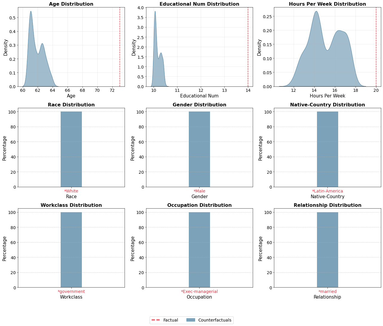
Figure 11: Feature distributions of generated counterfactual samples (blue shaded) with factual instance highlighted (red markers).

Prediction-risky samples.

To further investigate data samples near the decision boundary, we present the distributions of all features in the original dataset and the generated prediction-risky samples in Figure 12. These density plots provide a comprehensive view of the differences between the generated samples and the original data across multiple features. By analyzing these distributions, we can observe how the model identifies borderline cases based on different financial attributes. Across multiple features, the generated prediction-risky samples exhibit a much narrower distribution compared to the original data. This suggests that the model focuses on a specific subset of feature values when identifying borderline cases.

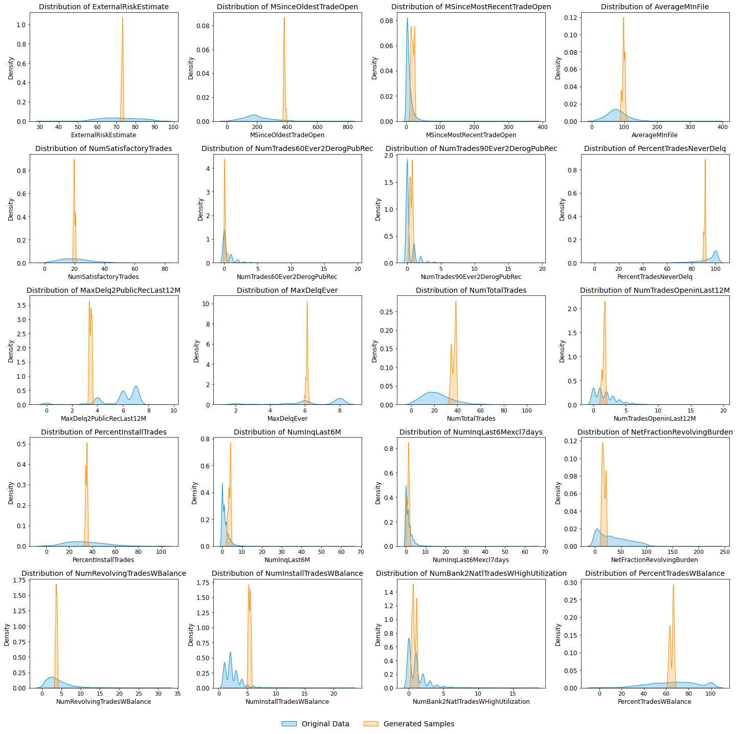
Figure 12: Feature distributions in the original data and generated prediction-risky samples.

Parameter-sensitive samples.

To complement the findings presented in Section 4, we provide the full set of feature distributions comparing parameter-sensitive samples and prediction-risky samples in Figure 13. These density plots illustrate how the two types of generated samples differ. By analyzing these distributions, we observe that while some features exhibit similar trends across both sample types, others show notable divergences. Features with broader distributions in parameter-sensitive samples indicate that model perturbations impact a wider range of instances.

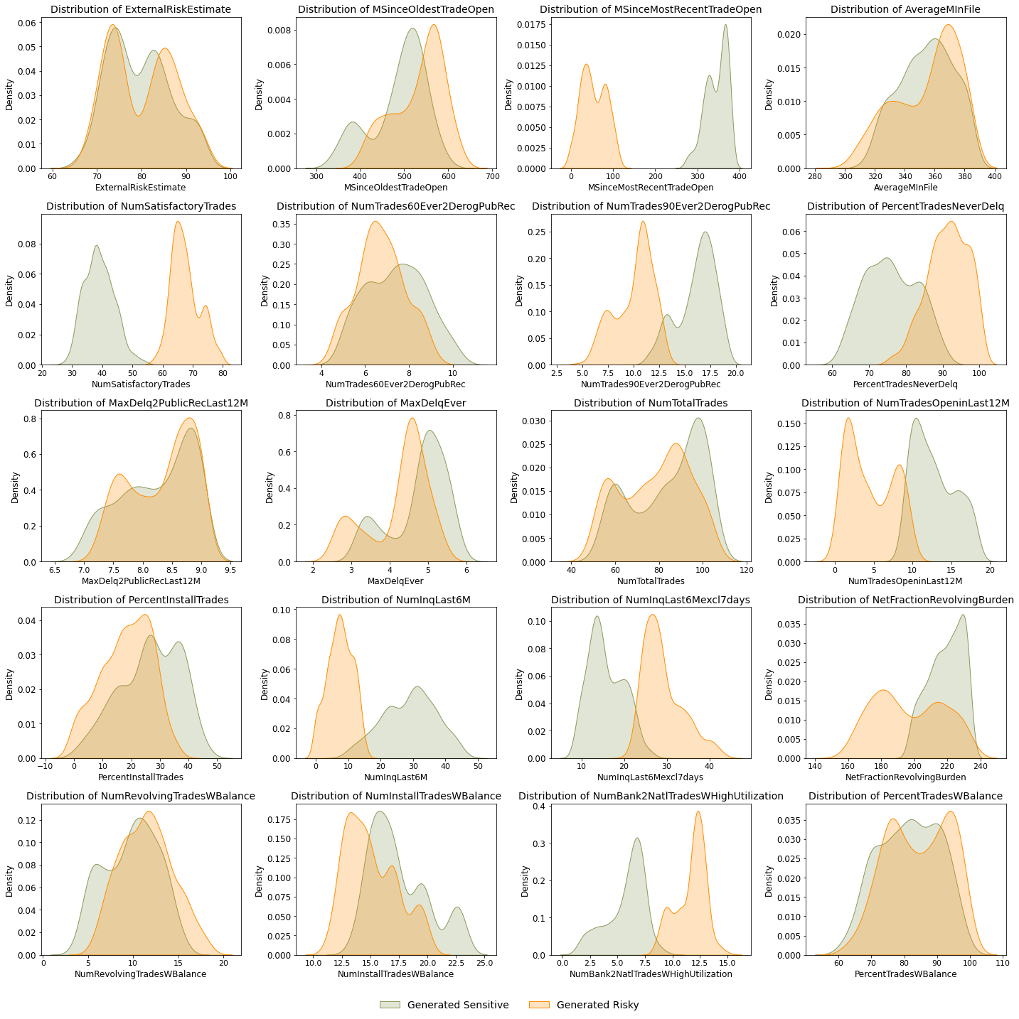
Figure 13: Feature distributions in generated parameter-sensitive and prediction-risky samples.

Appendix D The use of VAEs

A notable example of using pushforwards to obtain points on the data manifold comes from image datasets. We employ a VAE architecture with two convolutional layers each for the encoder and decoder submodules. Features in the convolutional layers are $32$ and $64$ with kernel sizes of (3,3) and a stride of (2,2). During training, the reconstruction loss is computed using bitwise entropy.

Figure 14 shows how this setup works for constructing loss functions $G$ on the latent space. One may use a combination of models, each precomposed with the decoder of the trained VAE. The resulting distribution on the latent space, after pushforwarding (i.e., passing the samples through the decoder), corresponds to a distribution on the data that is closer to the original data distribution.

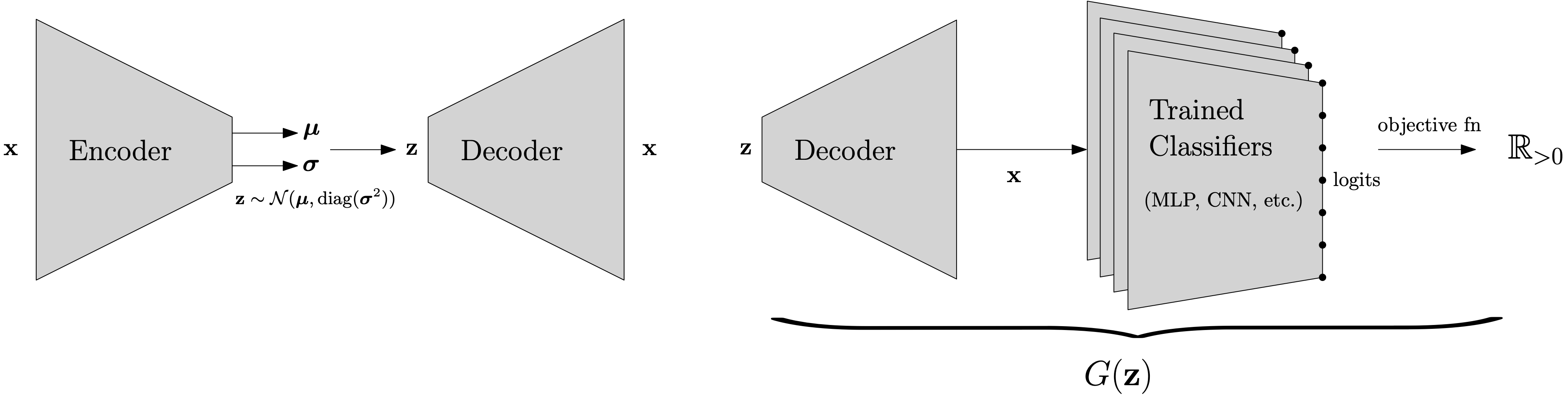
Figure 14: By precomposing with the decoder submodule of a trained neural network, we can define $G$ functions on the lower-dimensional latent space, while still leveraging networks designed for higher-dimensional image inputs.

References

- Arbel et al. (2021) Arbel, M., Zhou, L., and Gretton, A. Generalized energy based models. In International Conference on Learning Representations (ICLR), 2021.
- Becker & Kohavi (1996) Becker, B. and Kohavi, R. UCI Adult Dataset. UCI Machine Learning Repository, 1996. DOI: https://doi.org/10.24432/C5XW20.
- Biehl et al. (2016) Biehl, M., Hammer, B., and Villmann, T. Prototype-based models in machine learning. Wiley Interdisciplinary Reviews: Cognitive Science, 7(2):92–111, 2016.
- Breugel et al. (2024) Breugel, B. v., Kyono, T., Berrevoets, J., and van der Schaar, M. Decaf: generating fair synthetic data using causally-aware generative networks. In Proceedings of the 35th International Conference on Neural Information Processing Systems, NIPS ’21, Red Hook, NY, USA, 2024. Curran Associates Inc.
- de Rechtspraak (2020) de Rechtspraak. SyRI legislation in breach of European Convention on Human Rights, 2020. https://tinyurl.com/bdyxwsbb.
- Duvenaud et al. (2020) Duvenaud, D., Wang, J., Jacobsen, J., Swersky, K., Norouzi, M., and Grathwohl, W. Your classifier is secretly an energy-based model and you should treat it like one. In International Conference on Learning Representations (ICLR), 2020.
- Fawaz et al. (2018) Fawaz, H. I., Forestier, G., Weber, J., Idoumghar, L., and Muller, P.-A. Data augmentation using synthetic data for time series classification with deep residual networks. arXiv preprint arXiv:1808.02455, 2018.
- FICO (2018) FICO. Home Equity Line of Credit (HELOC) Dataset. FICO Community, 2018. https://community.fico.com/s/explainable-machine-learning-challenge.
- Goodfellow et al. (2014) Goodfellow, I., Pouget-Abadie, J., Mirza, M., Xu, B., Warde-Farley, D., Ozair, S., Courville, A., and Bengio, Y. Generative adversarial networks. In Advances in Neural Information Processing Systems, 2014.
- Joshi et al. (2019) Joshi, S., Koyejo, S., Vijitbenjaronk, W., Kim, B., and Ghosh, J. Towards realistic individual recourse and actionable explanations in black-box decision making systems. arXiv preprint arXiv:1907.09615, 07 2019.
- Kaggle (2021) Kaggle. Housing Prices Dataset, 2021. https://www.kaggle.com/datasets/yasserh/housing-prices-dataset.
- Kingma & Welling (2014) Kingma, D. P. and Welling, M. Auto-Encoding Variational Bayes. In 2nd International Conference on Learning Representations, ICLR 2014, Banff, AB, Canada, April 14-16, 2014, Conference Track Proceedings, 2014.
- Kusner et al. (2017) Kusner, M., Loftus, J., Russell, C., and Silva, R. Counterfactual fairness. In Proceedings of the 31st International Conference on Neural Information Processing Systems, NIPS’17, pp. 4069–4079, 2017.
- LeCun et al. (2006) LeCun, Y., Chopra, S., Hadsell, R., Ranzato, M., , and Huang, F.-J. A tutorial on energy-based learning. In Predicting Structured Data. MIT Press, 2006.
- LeCun et al. (2010) LeCun, Y., Cortes, C., and Burges, C. MNIST Handwritten Digit Database. AT & T Labs, 2010. http://yann.lecun.com/exdb/mnist.
- Liu et al. (2020) Liu, W., Wang, X., Owens, J. D., and Li, Y. Energy-based out-of-distribution detection. In Proceedings of the 34th International Conference on Neural Information Processing Systems, Red Hook, NY, USA, 2020. Curran Associates Inc.
- Ma et al. (2024) Ma, J., Dankar, A., Stein, G., Yu, G., and Caterini, A. Tabpfgen – tabular data generation with tabpfn. arXiv preprint arXiv:2406.05216, 2024.
- Margeloiu et al. (2024) Margeloiu, A., Jiang, X., Simidjievski, N., and Jamnik, M. Tabebm: A tabular data augmentation method with distinct class-specific energy-based models. arXiv preprint arXiv:2409.16118, 2024.
- Redelmeier et al. (2024) Redelmeier, A., Jullum, M., Aas, K., and Loland, A. Mcce: Monte carlo sampling of valid and realistic counterfactual explanations for tabular data. Data Mining and Knowledge Discovery, pp. 1830–1861, 2024.
- Ribeiro et al. (2016) Ribeiro, M. T., Singh, S., and Guestrin, C. “Why should i trust you?” Explaining the predictions of any classifier. In Proceedings of the 22nd ACM SIGKDD international conference on knowledge discovery and data mining, pp. 1135–1144, 2016.
- Shrikumar et al. (2017) Shrikumar, A., Greenside, P., and Kundaje, A. Learning important features through propagating activation differences. In International conference on machine learning, pp. 3145–3153. PMlR, 2017.
- van Breugel et al. (2021) van Breugel, B., Kyono, T., Berrevoets, J., and van der Schaar, M. Decaf: Generating fair synthetic data using causally-aware generative networks. In Ranzato, M., Beygelzimer, A., Dauphin, Y., Liang, P., and Vaughan, J. W. (eds.), Advances in Neural Information Processing Systems, volume 34. Curran Associates, Inc., 2021.
- Wachter et al. (2017) Wachter, S., Mittelstadt, B., and Russell, C. Counterfactual explanations without opening the black box: Automated decisions and the gdpr. Harv. JL & Tech., 31:841, 2017.
- Wong et al. (2016) Wong, S. C., Gatt, A., Stamatescu, V., and McDonnell, M. D. Understanding data augmentation for classification: When to warp? In 2016 International Conference on Digital Image Computing: Techniques and Applications (DICTA), pp. 1–6, 2016.
- Xu et al. (2018) Xu, D., Yuan, S., Zhang, L., and Wu, X. Fairgan: Fairness-aware generative adversarial networks. In 2018 IEEE International Conference on Big Data (Big Data), pp. 570–575, 2018.
- Zhao et al. (2017) Zhao, J., Mathieu, M., and LeCun, Y. Energy-based generative adversarial networks. In International Conference on Learning Representations (ICLR), 2017.