Cosmic electron spectra by the Voyager instruments and the Galactic electrostatic field
Abstract
The Voyager spacecrafts have been measuring since 2012 the rates of electron and nuclei of the cosmic radiation beyond the solar cavity at a distance of more than from the Earth. A record of unique and notable findings have been reported and, among them, the electron-to-proton flux ratio of 50 to 100 below energies of . This ratio is thoroughly opposite of that of 0.01 measured at higher energies in the range 10 to 10 . The difference amounts to four orders of magnitude. Arguments and calculations to show how this surprising and fundamental ratio lends support to the empirical evidence of the ubiquitous electrostatic field in the Milky Way Galaxy are presented. In other respects this paper examines and calculates, for the first time, the electric charge balance in the solar system delimited by the of the solar wind.
keywords:
cosmic rays in the Sun, solar modulation, Sun and stellar magnetic fields, electric fields in the solar system1 Introduction
A recent work provides empirical evidence of the Galactic electrostatic field [1]. A very short account of this work has been presented at the 37-th ICRC 2021, Berlin, Germany [2]. The Galactic electric field designated by (g for galactic) is permanent and ubiquitous except in regions where electrostatic shielding of structured ionized materials occurs. The solar system is one of this shielded region and, in spite of the electric shielding, highly specific effects with unmistakable signatures manifest themselves attesting the existence of the Galactic electric field . This paper deals with one of these effects, that is, the energy spectrum of cosmic electrons at low energies below and above measured by the Voyager spacecraft.
In essential terms and in other context, the negative electric charge of the electron spectrum, - , is just the electric charge needed to continuously neutralize the positive electric charge deposited by cosmic rays in the solar cavity. Hence this paper examines, calculates and reports, for the first time, the electric charge balance in the solar system within the of the solar wind.
A stuffy introduction is avoided here by relegating in the the new scientific context where the present paper properly shines.
According to the research book [3] published at the end 2022, , all stars of the retain a notable amount of positive electric charge deposited by the Galactic cosmic-ray nuclei. Charge deposition occurs by two different ways in two separate regions : the first way is the stopping of low-energy cosmic rays in the solar wind and the second way is the stopping of all cosmic rays of low and high energies in the body by ionization and nuclear interactions. By solar body is meant all the high density material residing within photosphere of radius ( for ). The electric charge per second deposited in the will be designated by ( for solar for wind) and ( for dense and for ), respectively. In the following the photospheric radius of the is and the massk inside so that the average density is 1.4 /. Anticipating successive results, above , = / (hereafter /) and = / in the range - of the cosmic-ray spectrum where data are available.
The region occupied by the solar wind is approximated by a sphere
of radius (sc for solar cavity). Its volume,
(4/3)
is a surrogate of the non spherical volume
delimited by the termination shocks of nominal radius of
observed by the Voyager Probes in two
different positions of the nearby circumstellar space [4, 5]. The
two positions in heliocentric system are degrees North at 94
AU [3] (Astronomical Unit, m) and -
degrees South at [4]. Crudely and nominally,
(94 + 84)/2 = = and
= (/) =
. In this work solar cavity is synonimous of solar cavern.
The electric charge deposition in the by cosmic nuclei mentioned above also apply to any stars as stellar winds are universal (see, for example, [6]).
2 Charge deposition in the solar wind region
Nuclei and electrons of the Galactic cosmic radiation intercepting the solar wind, in a sort of continuous fluid moving outwards, loose energy and a conspicuous fraction of the cosmic-ray flux with energies below - / is thoroughly arrested and dispersed in the environment.
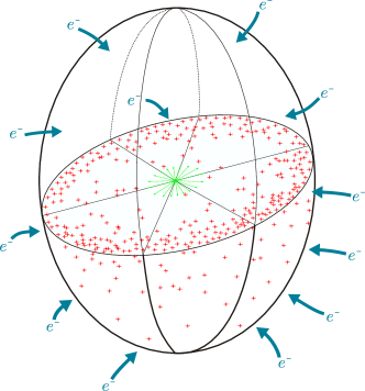
An artistic portrait of the electric charge deposited by cosmic rays in the solar wind is shown in fig. 1 by red crosses.
Let ( for terrestrial flux) denote the flux of cosmic rays measured at at the top of the atmosphere (zero atmospheric depth) and ( for demodulated) the unperturbed flux in the nearby interstellar space usually called demodulated flux. Solar modulation cyclically affects cosmic-ray intensity below - within the solar wind volume (see, for example, ref. [7]). The total amount of electric charge, deposited by cosmic rays in the volume occupied by the solar wind is given by :
| (1) |
where = = is the area intercepted by the demodulated flux of cosmic rays in the energy band and being . For protons = and for all cosmic nuclei at low energy = (see fig. 2 in ref. [8]). Of course, the electric charge deposited between the radius and the photosphere is missed in equation (1) and it has to be summed up. Here only notice that measurements of the cosmic-ray flux at - performed by recent and past space missions (Parker Solar Probe, Helios, Ulysses ) are available.
The demodulated spectrum besides nuclei include electrons , positrons and antiprotons so that the global positively charged cosmic-ray flux is, - + - . Traditionally in the literature the demodulated spectrum is also termed (LIS) but this is an interpretation of the demodulated spectrum, and not pure data, like energy spectra resulting from measurements are.
3 Charge balance around stars and multiple star systems
According to Potassium abundance in terrestrial meteorites [9] the cosmic-ray intensity in the last 2 billion years has maintained approximately constant. This datum is regarded as solid input here to state, or posit, the quasi stationary state in the flows of the electric charge in the volume .
At the arbitrary time interval , the positive electric charge deposited in the volume amounts to : ( + ) .
The neutralization of the positive charge excess during the time span , + in the volume promotes a quiescent electron current designated by and called migration current. The electric current is qualitatively represented by the thick blue arrows in fig. 1. The current entering the solar cavity coming from the nearby interstellar space, beyond the radius , transports the negative electric charge = in the arbitrary time interval . For an ideal, continuous isotropic current and a spherical solar cavity it would be : () = . The total electric charge contained in the solar cavity of volume in the time interval is given by :
| (2) |
where (0) is the total electric charge in the volume at initial time = 0. Any arbitrary time may be chosen as initial time or zero time taking into account the age of about . The charge within the volume = at time is denoted by ().
The stationary state during the time interval posits, + + = and, therefore, (0) = () where () designates the residual electric charge at the time . For instance, during the temporal span surveyed by Potassium data [9] of , the residual charge () remained constant and the time = , i.e. the initial time of the present calculation is back in time from the present epoch.
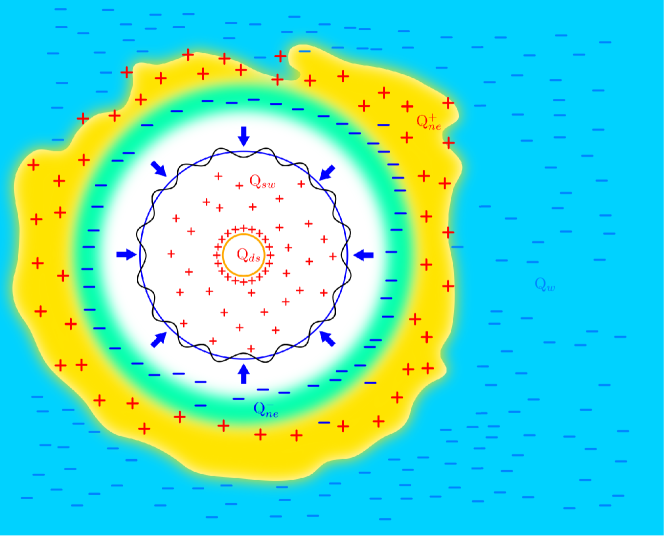
If the average displacement velocity of the migration current were very high, ultimately, comparable to , the light speed, a rapid neutralization of the positive electric charge ( + ) = ( + ) within the volume at any arbitrary time spans t would take place. In this imaginary and unphysical condition the residual charge () in equation (2) would turn out to be (0). The neutralization of the positive electric charge, + requires a characteristic time interval ( per neutralization) regulated by the conductivity of the circumstellar medium, the distance of the cosmic-ray sources, the convective motion of local materials, moving charged plasma parcels, moving neutral plasma pockets in the environment, the local magnetic fields, local electrostatic fields, the electrostatic field of the star surfaces and in the solar wind region and other parameters. During the time span the negative charge transported by quiescent electrons surrounding nearby stars and nearby clouds (see fig. 3) uncovers the positive quiescent charge in a larger circumstellar ambient so that : + = 0, based on charge conservation in a finite volume of the adjacent larger ambient surrounding the tiny solar cavity.
How much electric charge did the nascent store before emanating solar wind ? If the time = 0 is set at 4.567 back in time (nominal age), then the term () in equation (2) would represent the pristine, presolar electric charge at the birth.
Due to the finite neutralization times (), the positive electric charge () accumulates implying () (). Ultimately, () will be neutralized by a fraction of the negative electric charge = dispersed in the cosmic-ray sources in the whole Galactic disk. This negative charge are orbital electrons lost by the accelerated cosmic nuclei in all Galactic cosmic-ray sources. These particular orbital electrons are designated in the twin works [1, 3] by the new term, . The term is useful whenever charge balance of various particle populations including cosmic rays has to be examined and calculated. This point is debated in of ref. [1].
Taking into account the total negative charge of widow electrons and the positive charge of cosmic-ray nuclei being = - = , a more rigorous expression of equation (2) may be written in this way :
where is the nominal negative charge of widow electrons in the volume and the nominal positive charge of cosmic-ray nuclei in the same volume . Therefore, the nominal negative charge of would be () = - and + () less than this value because the positive charge is dispersed in a volume larger than that of the disk (see next Section ).
Notice that sources of electric charge within the solar cavity do not alter the stationary state envisaged above. For example, Jupiter planet releases electrons [10, 11] observed at by at a rate of some electron/ in the range - [11]. Charge conservation requires a corresponding positive electric charge in situ in the Jupiter planet. Other known sources of negative charge within are sporadic emission of energetic electrons during solar flares.
4 The equilibrium of the electric currents in the heliosphere
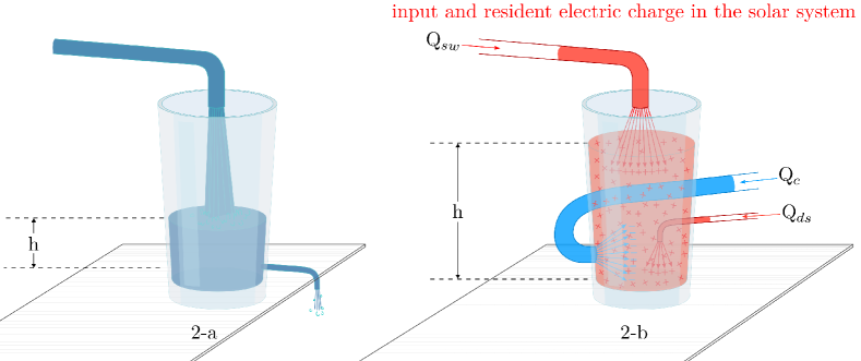
The electric charges t and t stored in the and solar wind, respectively, during the time span t produce distinctive physical effects. For example, as the charge rotates with the , it has to generate a magnetic field. This effect is presented in 6.
The basic condition of the charge balance expressed by equation (2) is the stationary state or steady condition or equilibrium. In this condition, in the volume = , electric currents equilibrate e.g. + + = and the baseline charge, (t) = () + () + () is not zero but it assumes some finite value as depicted in fig. 2-a by an hydraulic analogy. In the steady-state condition at the arbitrary time span , regardless of the complexity of the environment, the neutralization charge entering the solar cavity from the adjacent interstellar space (see fig. 3) has to equalize the positive electric charge ( + ) deposited by cosmic nuclei in the same volume and same time span . This neutralization is certainly influenced by the permanent charge (). The equilibrium implies that the number of quiescent electrons of extremely low energy entering the solar cavity has to swamp that of quiescent protons and quiescent nuclei in the same energy band because of the overwhelming positive charge entering the solar cavity via cosmic nuclei of higher energies, above as attested in fig. 4.
Notice that the nominal charge of widow electrons in the solar cavity, (), is thoroughly negligible compared to the charge + deposited by cosmic nuclei. As the average charge density of widow electrons in the Galactic disk of volume is, / = - / = - / [1] and the volume of the spherical solar cavity is = , nominally, the total negative charge (/) is about , thoroughly negligible relative to any plausible estimate of and . For example, by setting the lifetime of cosmic rays in the Galaxy, = years = , it results = = = and = = = , respectively, which outnumber () limited to .
As local electric fields exist in interstellar clouds as also pointed out by
others and the solar system is embedded in the nearby clouds 222The volume of the space adjacent to the solar cavity is insignificant relative to that of the of some . The surrounding the has a size of about , gas density / and temperature of . The Local Interstellar Cloud embraces the in a wider ambient, about in size, and other bubbles called , and lie in the vicinity. The precious, unique and historical results of the on magnetic fields, gas density, pressure, solar wind features and others are expected to vary in these larger regions because the static and dynamic conditions of matter and radiation are different. Thus, measurements of the refer indeed to the very skinny region around a G star, the , and extrapolations of these measurements to the huge and variegated interstellar space might be insecure. , quiescent electrons of the indifferentiated interstellar medium are accelerated and decelerated with multiple gains and losses of kinetic energies in a wide range of values. For example, a local electric field of / acting in an unshielded milliparsec region ( ) imparts of kinetic energies to charged particles. This implies that the neutralization charge of quiescent electrons most likely occurs not at thermal or suprathermal energies ( ), in the band, but at higher energies due to the ubiquitous presence of local electrostatic fields.
5 The positive electric charge stored in the solar cavity
The intensity of cosmic nuclei versus time during the magnetic solar cycle of 22 years enables to infer the intensity of cosmic nuclei in the outer space surrounding the solar cavity. The energy spectra of the cosmic radiation are called ( ) or demodulated spectra, or, eventually, energy spectra of the very local interstellar medium () as hinted earlier.
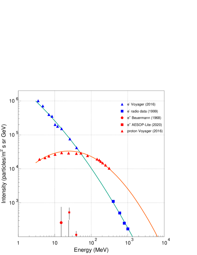
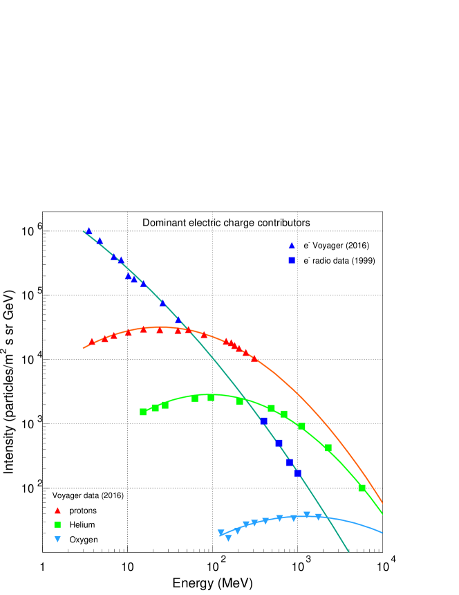
The most recent advance on the measurements of the electric currents and have been made by the and Voyager detectors which directly determine cosmic-ray fluxes in the very local interstellar medium. The energy spectra of cosmic proton and electron are shown in fig. 4. The electron spectrum from radio data [13] in the interval to (blue squares) shown in fig. 4 intrinsically constitutes the demodulated spectrum and, in this particular case, appropriately termed spectrum.
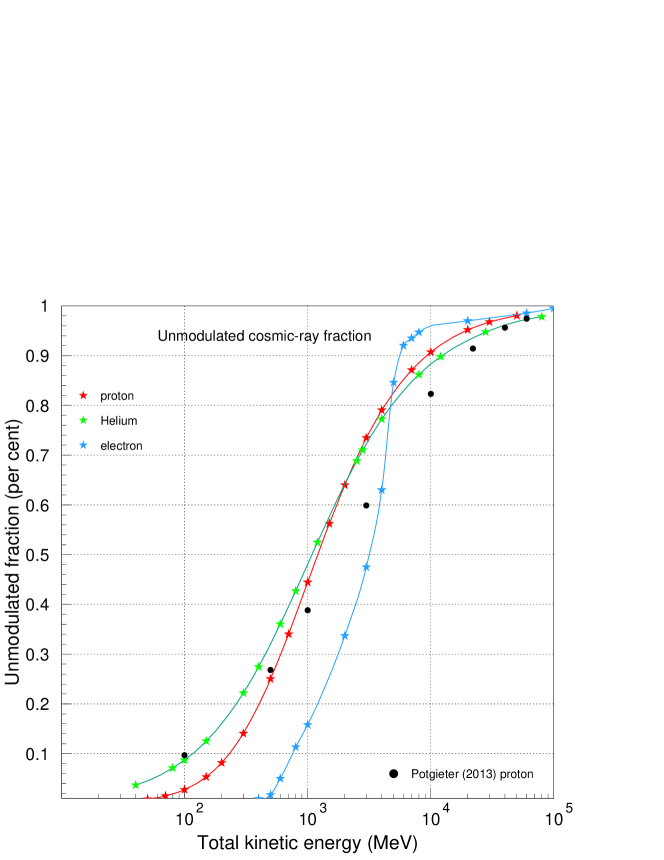
Cosmic protons in the range - entering the solar cavity have a flux of part/ according to the observed spectrum shown in figure 4 and 5. Due to the solar modulation only a fraction of these protons contributes to the current . The fraction depends on the energy and it is intended to be the average value in many solar cycles of 22 years. The fraction is shown in figure 6 according to observations collected in the last 70 years. The proton fraction is called unmodulated proton fraction. The positive charge lost by cosmic protons in the volume due to the flux is : = / where = , = , = and = . Details of the calculation are given in the .
Cosmic electrons in the same energy range - have a flux of part/ according to the observed spectrum shown in figure 4 and 5. The unmodulated electron fraction, , versus energy is given in figure 6. The negative charge entering the volume corresponding to this flux is /. Therefore, the global electric charge balance of proton and electron in the range - is + /.
Proton and electron spectra shown in figures 4 and 5 intercross around . This energy represent a critical divide : above the total electric charge entering the solar cavity via cosmic rays is always positive while below is always negative. In the range - the global input charge of proton and electron is negative, - / while that above is positive, being + /.
In the global charge balance across the solar cavity positrons and antiprotons at low energies have to be included. In the critical range to no measurements of these antiparticles in the interstellar medium are available. Thus, only tentative extrapolations of the modulated spectra observed at Earth might be used.
The antiproton flux in the energy range to remains unmeasured. Just above the / flux ratio is about [14] reaching a stable plateau of about above . Loose upper limits of about at the maximum explored energies of - have been reported [15] using the standard Moon shadowing technique. As antiprotons are secondary particles generated by interactions of cosmic nuclei in the and no obvious sources are known, the negative charge from antiprotons entering the solar cavity is negligible compared to that of low-energy cosmic electrons.
Cosmic positrons are secondary particles generated by interactions of cosmic nuclei in the , but unlike antiprotons, Galactic quiescent positron sources do exist located in stars and supernovae remnants. These sources are the radioactive nuclides , and which yield positrons in the range while decaying.
Important measurements of positron flux below at Earth were performed in 1968 by the - detector [17] and in 2018 during the positive magnetic polarity of the cycle by the AESOP-Lite detector in the energy band to [18]. Data points of the highest rates of these two experiments are shown in fig. 4. Positron electric charge, in principle, might challenge the dominance of negative electric charge carried by electrons in the range - (see fig. 4).
Similarly to equation (1) the charge of the positive positron current, , is computed by : .
In principle low energy positrons from radioactive decays of , and might be trapped in local electric fields debouching in flux spikes at very low energies in the band 1 to 50 thereby affecting the neutralization of the positive charge . Should the positron current be comparable to the migration current , the postulated neutralization around the becomes questionable.
6 Electric charges stored by stars are consistent with the observed stellar magnetic fields
From the previous analysis follows that a current of negative charges of quiescent electrons called in the work [1] and depicted in fig. 1 has to enter stellar cavities of any stars to neutralize the positively charged currents, + certainly deposited by cosmic rays.
Moving charges generate magnetic fields of definite strengths and shapes. As stars retain positive electric charge and move at high velocities, both rotating and translating, smooth magnetic fields sprout everywhere. Here the focus is on the fact that measurements of magnetic field strengths of various stellar categories and are consistent with rotating electric charges in the range - with typical rotational periods - [19].
The surface receives from the cosmic radiation the positive charge per second = / computed by = a/ with a = 28656 part/ [1], = [1], a threshold energy = , arbitrarily large being not influential, = [8] and = the collecting area. The threshold energy of seems in the correct range taking into account solar modulation. For example, a threshold of 10 would result in = /.
As particle density in the is close to / from 1.4 // , being exceedingly high relative to the electron density of the migration current, the neutralization of the charge occurs , i.e. cosmic nuclei extinguished within solar photosphere absorb quiescent electrons from local solar materials. If no charge neutralization from external sources takes place, the requirement of charge conservation within the radius would yield an unlimited accumulation of positive charge as electrons from the from the local interstellar medium are thoroughly absorbed by the ionized atoms of the solar wind and cannot reach the main body which resides within the tiny radius of = face to of .
For example, in one billion years ( = ) assuming no charge neutralization from the migration current , the accumulated charge in the would amount to = . Notice further that prestellar materials do certainly store positive electric charges deposited by cosmic rays as argued elsewhere (see and of ref.[1]). This pristine charge deposition occurring in the nascent certainly adds to the charge computed above. With no charge neutralization, ineluctably, magnetic field intensities in stars have to augment with time until charge densities saturate the hosting and absorbing structures eventually enabling new discharge channels.
Global magnetic fields resulting from spinning charges can be estimated by assuming a simple loop of current of radius . The order of magnitude of the field strength is, = / ( ) where is the radius of the star. Measured star rotation periods range from to days (see data of stellar rotational periods in of ref. [19]19-vidotto; also fig. 6 in Reiners). For example, the rotation period is days, so that, after one billion year, = / = . The magnetic field strength of the rotating charge from the formula above is : = / = = . In the quiet the overall magnetic field strength is in this range [20] and, similarly, in other stellar categories [21].
Perhaps the best measurements of magnetic field intensities in stars are those in binary systems. Magnetic flux conservation is invoked during stellar explosions in binary systems. Such explosions yield neutron stars. The typical radius of collapsed stars is about while that of a neutron star about . In a spherical geometry the ratio of the areas is which is the enhancement factor of the magnetic field. Magnetic field strengths measured in neutron stars are in the range - and, consequently, with a reduction factor of , those in collapsing parent stars in binary systems are in the range - .
These magnetic field strengths are also measured, order of magnitude, in the quiet Sun [20], in , , and stars [21] and and stars [22]. A sample of magnetic field strengths measured in and stars conform to a lognormal distribution with an average value of 338 .
It is worth recalling that magnetic field strengths measured in the spots, flares and energetic outbursts from the surface and other star surfaces are approximately - , some 2 to 3 orders of magnitude higher than - . As magnetic field intensities in stars in quiet conditions unambiguously differ from those measured in magnetic spots, the nexus between rotating charges and magnetic field intensities is highly suggested or tentatively demonstrated.
In order to explain magnetic fields in stars, aside from spinning positive charges , other mechanisms have been proposed such as the dynamo theory quite recurrent in the literature.
Neutron stars result from the explosion of massive stars which have magnetic field strengths of some believed to be originated by the classical dynamo mechanism. As magnetic flux during explosion conserves, field strengths in neutron stars have enhanced magnetic fields by a rough factor of , as previously noted. Do magnetic fields in neutron stars also originate via dynamo mechanism ? This mechanism seems inapplicable to neutron stars which hardly might host the large convective cells of normal stars due to the small sizes of about 10 . Conceivably, rotating positive charges appear to be a more natural explanation of both magnetic fields in progenitor star and neutron star.
7 Compendium and Conclusion
It is an assessed fact that cosmic rays arriving at Earth are arrested in the solar wind thereby depositing a positive electric charge at all the energies above (see fig. 4) according to the Voyager data. The positive electric charge per second deposited by cosmic-ray nuclei (proton and helium) in the solar cavity of nominal radius = [3, 4] has been calculated in and of this work and it amounts to = /. The estimated current is likely to be correct within a factor of 2.
This charge has to be neutralized in order to avoid electric fields of very high intensity within the solar wind volume 333The electric field generated by the permanent electric charge residing in the solar cavity is immersed in a bath of moving ions, namely, the solar wind, which tends to shield and, consequently to obscure any electrostatic effects. In spite of that, during transient phenomena within the solar wind itself or perturbations originated outside the solar wind volume, shielding may be inefficient or absent. In this case electron acceleration and nucleus acceleration within the solar wind have to manifest. Indeed, proton and Helium acceleration in the range 0.1- in the interplanetary medium has been observed long time ago [23]; it was unpredicted and erroneously attributed to non electric acceleration processes. A population of energetic electrons in the solar wind in the interval - during quiet time conditions has been also reported and its acceleration is not in the Sun [24] but in the interplanetary space. It is worth noting that quite time conditions indicate absence of compressions, absence of shocks in the medium and no sudden ambient alterations. and its environment. Sources of electric charge within the solar cavity in a finite, specified volume, for example Jovian electrons [10, 11], conserve electric charge and, accordingly, cannot neutralize over adequate, long time intervals. It follows that the electric charge has to come from the exterior of the solar cavity as qualitatively depicted in fig. 1 by blue arrows pointing inward representing entrant negative charge (electrons). The motion of these low energy electrons and their inherent electric currents in the whole Galaxy, gives rise to the denoted by as asserted in this work and motivated elsewhere [1, 2]. The pristine spatial origin of the is in all cosmic-ray sources in the Galaxy as amply debated in ref. [1].
The neutralization of the positive charge in the arbitrary time interval within the solar cavity of nominal radius of [3, 4] = requires an equal amount of negative charge designated here by = to be established by measurements. Ideally, in steady state flows = where is the migration current based on a logical inference amply debated in the work [1], as mentioned earlier. The notion of derives from the necessity to neutralize the electric charge deposited by cosmic nuclei extinguished in the Galaxy. The Sun offers a unique opportunity to measure the electric charge balance of cosmic rays around one star and, hence, to observe one around a single star and not the of the Galactic stars which globally generate the Galactic magnetic field (see ref. [1]; 14 and 15).
It is an impressive and notable fact that the negative current has been detected by the Voyager instruments and by measuring huge rates of energetic electrons in the range to (see fig. 4) while exiting the solar cavity beyond the shell region denoted [25].
The negative electric charge per second in the range - entering the solar cavity is - / derived in and from the cosmic-ray electron spectra measured by the Voyager detectors. This negative charge surprisingly counterbalances the positive electric charge per second deposited by cosmic rays in the solar cavity, + , of / in the range - . Within the accuracy of the calculation, the missing negative charge labeled here necessary for a perfect charge neutrality, namely, - + + = 0 is - /. This charge amount is not incompatible with the electron spectra in the range - constrained by the Pioneer data [26] and low frequency radio data [13] as speculated by others in the solar modulation arena (see, for example, ref. [26] for a plausible electron spectrum in this unexplored energy range).
In some respects the postulated dominance of cosmic electrons over nuclei below is both impressive and surprising 444The surprise has been vented by those who made the measurements like William R. Webber of the Las Cruces University, New Mexico, a colleague of balloon experiments of bygone days (see for example ref. [27, 28]). In fact, he asserts [29]: ” the ratio of the electron to nuclei intensities in , e/H(E), measured up to by outside the heliosphere…At 2 this e/H(E) ratio is 100 (yes !) decreasing to at . ” because cosmic rays above solar modulation energies, i.e. - , exhibit the opposite trend, namely, fluxes of protons and heavier nuclei dominate those of cosmic-ray electrons. The energy of above is the maximum measured cosmic-ray electron energy to day (2025).
In the census of electric charges within the finite volume and arbitrary time span , the charge absorbed inside the photosphere within , namely , is negligible but it appears quite adequate to generate stellar magnetic fields as loomed out in .
Along the same logical framework of this calculation it emerges that rotating electric charges stored by stars due to the charge deposition of cosmic rays generate magnetic field strengths in the range - with dipolar geometry which are in accord, order of magnitude, with spectropolarimetric Zeeman data of stars and radio observations of magnetic fields of neutron star progenitors as debated in . The agreement of computed and observed magnetic field intensities of about - further supports the context of this work.
Appendix A
The novel scientific context in Cosmic Ray Physics
According to the works [1, 2] the has a pervasive and stable electrostatic field designated by (g for galactic) generated by the motion of positively and negatively charged particles of the cosmic radiation. Cosmic rays are accelerated by the electrostatic field which performs the acceleration from quiescent energies up to the maximum energies of of cosmic Uranium nuclei [30]. In restricted regions of the the field is shielded by ionized materials as, for instance, the region occupied by the solar wind in the solar system.
Facts supporting the existence of the electrostatic field discussed in [1] are : (1) the constant spectral index of the overall cosmic-ray energy spectrum comprised between 2.64-2.68 up to energies of ; (2) the maximum energies of Galactic protons of ; (3) the chemical composition of the cosmic radiation above the energy of which has to consist only of heavy nuclei; (4) the intensity, orientation and direction of the Galactic magnetic field; (5) the absence of correlation of the arrival directions of ultra-high-energy cosmic rays in the interval - with powerful radio galaxies in the nearby universe. As cosmic rays are Galactic up to , the absence of correlation is a natural, obvious in the context of the novel picture of the cosmic radiation reported in the works [1, 2, 3].
The calculated features (1), (2), (3), (4) and (5) impressively agree with the experimental data as debated and highlighted in the aforementioned research book [1]. By contrast, results and predictions recurrent in the past and present literature of the traditional theories of the cosmic radiation are severely inconsistent with the facts (1)-(5). For example, the bulk motion of cosmic rays in the erroneous traditional theories is thoroughly disconnected from the geometrical pattern of the Galactic magnetic field.
Probably, the most outstanding result in terms of accord between data and calculation reported in [1], designated fact (4) above, is the exact account of the regular magnetic field of the with its intensity of - and its variegated and unique geometrical pattern in all the Galactic volume and beyond. The remarkable accord with the optical and mostly radio data is described in and of ref. [1].
Presently a conspicuous fraction of scientific community believes that cosmic rays are accelerated in supernova remnants up to - by a mechanism called diffusive shock acceleration. Numerous and variegated experimental data disagree with this credence. These inconsistencies are presented and debated in the Appendix of ref. [1] and in the research book [31] : .
Appendix B
The modulated spectra of electron, proton and Helium
In to preserve a simple calculation scheme of the electric charge balance in the solar cavity, namely, + , only electrons and protons have been considered. Here two necessary extensions of the calculation : (1) the effect of the solar modulation on the energy spectra ; (2) the inclusion of Helium in the charge budget, the third major charge source in the solar cavern. The next contributing heavier nucleus is Oxygen. Its charge input, according to the data shown in figure 4, is less than 8 per cent of the charge input of proton and Helium and therefore negligible for the aim of this work.
The analytical representation of the demodulated spectrum, , anchored to the observational data of Voyager Probes [17] and radio data [13] allow a reliable evaluation of the . These factors quantify the amount of the observed flux of energy (total kinetic energy) arrested in the solar cavity, namely, = / where J is the measured terrestrial flux or that in another location within . The modulation region goes from the Sun photosphere up to 112 AU [4, 5].
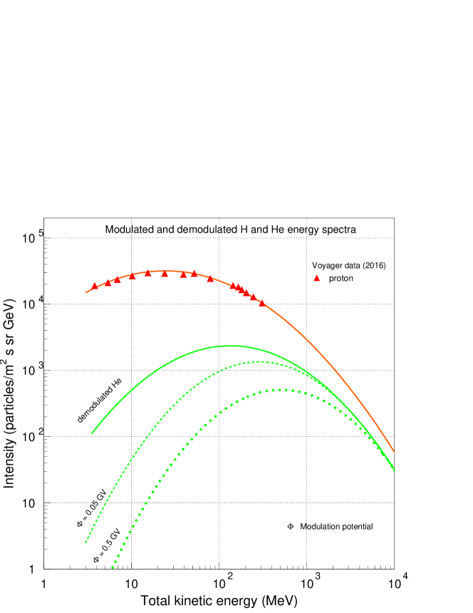
Since half a century it is known that the intensity variations of proton and Helium registered on Earth in the range of - , between minimum and maximum modulating conditions, span a factor of about -. This basic fact remains true to day after exploring 4 solar cycles. The spectra displayed in figure 7 are an example of computed modulation of Helium according to a classical parametrization [33] adopted in this work.
Electron and proton charge flows are given in . Here are those of Helium.
Helium in the range - entering the solar cavity have a flux of part/ according to the observed spectrum shown in figure 5. Due to the solar modulation only a fraction of Helium nuclei, , contributes to the current . The fraction depends on the energy and it is intended to be the average value in many solar cycles of 22 years. The fraction is shown in figure 6 according to observations collected in the last 70 years. The positive charge lost by Helium in the volume due to the flux is : = / where = , = , = and = . Thus, the He charge input is percent of that of the proton.
For comparison with proton and electron, in the range - , the global input charge is , / while that in the range - is /.
The modulation factors shown in figure 7 are obtained by the demodulated spectra (often called for Local Interstellar Spectra) and measured spectra at Earth, or close to it. As the Earth is located at 1 additional electric charge deposition occurs between the and the Earth. As the spherical volume enclosed by the Earth radius to the is only a fraction of of that of the solar cavern, this charge deposition is neglected in this work. Notice also that a severe conflict between measured and computed radial cosmic-ray gradients emerged in the inner heliosphere making uncertain plain extrapolations of charge deposition based on the outer heliosphere data.
The dominant error source in the evaluation of charge + comes from the electron spectrum below which is unmeasured but highly constrained by radio data [13] and Pioneer 10 observations [34] made at 70 AU for electron energies of 2-20 . The limit of above is an intrinsic limitation at low energy of the and Voyager instruments.
Appendix C
Failures of diffusion equation applied to cosmic rays
In principle the omission of the Galactic electrostatic field in any calculation of the properties of Galactic cosmic rays has to conduct to severe inconsistencies with observational data. Here some conflicts between computed and observed cosmic-ray features are mentioned. The computed features are obtained by the of used since more than 70 years. These conflicts are commonly registered in the literature.
(1) The Boron-to-Carbon flux ratio in the range - is inconsistent with standard calculations ( see fig. 9 of ref. [12]).
(2) According to the Voyager Team [12] the and isotope spectra in the range - / severely disagree with those computed by the simulation code of Galactic cosmic rays in spite of the fine tuning of simulation parameters. In the energy band - / the observed intensity of is higher than that computed by code by more than an order of magnitude. The GALPROP code adopt the diffusion equation tuned, in this case, at low energies around 0.005-20 /.
(3) The ionization rate of Hydrogen termed ( for cosmic rays) computed with the reconstructed cosmic-ray energy spectrum in Galactic environment via amounts to (-) [12]. It differs by more than an order of magnitude from the ionization rate extracted from chemical reactions in the interstellar medium, namely, ( for chemical) = [34]. The reconstructed energy spectrum of cosmic rays in Galactic environment is derived from the diffusion equation with its highly abstract and unrealistic scheme.
(4) The diffusion equation of cosmic rays in the predicts a decreasing ratio of the antiproton-to-proton flux ratio (/) above the energy of 2.6 . On the contrary, recent and past data in the interval - show a flat / ratio incompatible with calculations.
Additional evidence of the inadequacy of current ideas to describe low-energy cosmic rays, solar energetic particles and other solar phenomena is elsewhere [32].
References
- [1] A. Codino, The ubiquitous mechanism accelerating cosmic rays at all the energies, Società editrice Esculapio, Bologna, 2020.
- [2] A. Codino, The ubiquitous mechanism accelerating cosmic rays at all the energies, in: 37th International Cosmic Ray Conference, 2022, p. 450. arXiv:2109.04388, doi:10.22323/1.395.0450.
- [3] A. Codino, How electrostatic fields generated by cosmic rays cause the expansion of the nearby universe, Società editrice Esculapio, Bologna, 2022.
- [4] E. C. Stone, et al., Voyager 1 Explores the Termination Shock Region and the Heliosheath Beyond, Science 309 (5743) (2005) 2017–2020. doi:10.1126/science.1117684.
- [5] J. D. Richardson, et al., Cool heliosheath plasma and deceleration of the upstream solar wind at the termination shock, Nature 454 (7200) (2008) 63–66. doi:10.1038/nature07024.
- [6] R.-P. Kudritzki, J. Puls, Winds from Hot Stars, Annual Review of Astronomy and Astrophysics 38 (2000) 613–666. doi:10.1146/annurev.astro.38.1.613.
- [7] I. G. Usoskin, et al., Solar modulation parameter for cosmic rays since 1936 reconstructed from ground-based neutron monitors and ionization chambers, Journal of Geophysical Research (Space Physics) 116 (A2) (2011) A02104. doi:10.1029/2010JA016105.
- [8] A. Codino, The dominance of secondary nuclei in the cosmic radiation and the modulation of the nuclear species at the injection of the galactic accelerator, in: 34th International Cosmic Ray Conference (ICRC2015), Vol. 34 of International Cosmic Ray Conference, 2015, p. 488. doi:10.22323/1.236.0488.
- [9] H. Voshage, et al.H. Feldmann, O. Braun, Investigations of cosmic-ray-produced nuclides in iron meteorites: 5. More data on the nuclides of potassium and noble gases, on exposure ages and meteoroid sizes., Zeitschrift Naturforschung Teil A 38 (1983) 273–280. doi:10.1515/zna-1983-0227.
- [10] J. Lheureux, P. Meyer, Quiet-time increase of low-energy electrons the Jovian origin., The Astrophysical Journal 209 (1976) 955–960. doi:10.1086/154794.
- [11] D. Moses, Jovian Electrons at 1 AU: 1978–1984, ApJ 313 (1987) 471. doi:10.1086/164987.
- [12] A. C. Cummings, et al., Galactic Cosmic Rays in the Local Interstellar Medium: Voyager 1 Observations and Model Results, ApJ 831 (1) (2016) 18. doi:10.3847/0004-637X/831/1/18.
- [13] J. D. Peterson, A New Look at Galactic Polar Radio Emission and the Local Interstellar Electron Spectrum, in: D. Kieda, M. Salamon, B. Dingus (Eds.), 26th International Cosmic Ray Conference (ICRC26), Volume 4, Vol. 4 of International Cosmic Ray Conference, 1999, p. 251.
- [14] K. Abe, et al., Measurement of the Cosmic-Ray Antiproton Spectrum at Solar Minimum with a Long-Duration Balloon Flight over Antarctica, Physical Review Letters 108 (5) (2012) 051102. arXiv:1107.6000, doi:10.1103/PhysRevLett.108.051102.
- [15] B. Bartoli, et al., Measurement of the cosmic ray antiproton/proton flux ratio at TeV energies with the ARGO-YBJ detector, Phys. Rev. D 85 (2) (2012) 022002. arXiv:1201.3848, doi:10.1103/PhysRevD.85.022002.
- [16] M. S. Potgieter, R. D. T. Straus, At What Rigidity Does the Solar Modulation of Cosmic Rays Begin?, in: International Cosmic Ray Conference, Vol. 33 of International Cosmic Ray Conference, 2013, p. 2417. arXiv:1308.1614, doi:10.48550/arXiv.1308.1614.
- [17] K. P. Beuermann, et al., Cosmic-Ray Negatron and Positron Spectra Between 12 and 220 MeV, Physical Review Letters 22 (9) (1969) 412–415. doi:10.1103/PhysRevLett.22.412.
- [18] S. Mechbal, et al., Measurement of Low-energy Cosmic-Ray Electron and Positron Spectra at 1 au with the AESOP-Lite Spectrometer, ApJ 903 (1) (2020) 21. arXiv:2009.03437, doi:10.3847/1538-4357/abb46f.
- [19] A. A. Vidotto, et al., Stellar magnetism: empirical trends with age and rotation, Monthly Notices of the RAS 441 (3) (2014) 2361–2374. arXiv:1404.2733, doi:10.1093/mnras/stu728.
- [20] J. Sánchez Almeida, et al., Solar Polarization 6, Vol. 437 of Astronomical Society of the Pacific Conference Series, 2011, p. 451. arXiv:1105.0387, doi:10.48550/arXiv.1105.0387.
- [21] S. I. Plachinda, T. N. Tarasova, Precise Spectropolarimetric Measurements of Magnetic Fields on Some Solar-like Stars, ApJ 514 (1) (1999) 402–410. doi:10.1086/306912.
- [22] A. F. Kholtygin, et al., BOB Collaboration, Statistics of Magnetic Field Measurements in OB Stars, in: Y. Y. Balega, D. O. Kudryavtsev, I. I. Romanyuk, I. A. Yakunin (Eds.), Stars: From Collapse to Collapse, Vol. 510 of Astronomical Society of the Pacific Conference Series, 2017, p. 261. arXiv:1701.00739, doi:10.48550/arXiv.1701.00739.
- [23] F. B. McDonald, et al., The interplanetary acceleration of energetic nucleons., ApJl 203 (1976) L149–L154. doi:10.1086/182040.
- [24] R. P. Lin, WIND Observations of Suprathermal Electrons in the Interplanetary Medium, Space Science Reviews 86 (1998) 61–78. doi:10.1023/A:1005048428480.
- [25] E. C. Stone, et al., Voyager 1 Observes Low-Energy Galactic Cosmic Rays in a Region Depleted of Heliospheric Ions, Science 341 (6142) (2013) 150–153. doi:10.1126/science.1236408.
- [26] U. W. Langner, et al., Proposed local interstellar spectra for cosmic ray electrons, in: International Cosmic Ray Conference, Vol. 10 of International Cosmic Ray Conference, 2001, p. 3992.
- [27] R. L. Golden, …, A. Codino, et al., Observations of Cosmic-Ray Electrons and Positrons Using an Imaging Calorimeter, ApJ 436 (1994) 769. doi:10.1086/174951.
- [28] M. T. Brunetti, A. Codino, …, W. R. Webber, et al., Negative pion and muon fluxes in atmospheric cascades at a depth of 5 g ?, Journal of Physics G Nuclear Physics 22 (1) (1996) 145–153. doi:10.1088/0954-3899/22/1/014.
- [29] W. R. Webber, T. L. Villa, A Comparison of the Galactic Cosmic Ray Electron and Proton Intensities From 1 MeV/nuc to 1 TeV/nuc Using Voyager and Higher Energy Magnetic Spectrometer Measurements Are There Differences in the Source Spectra of These Particles?, arXiv e-prints (2018) arXiv:1806.02808arXiv:1806.02808, doi:10.48550/arXiv.1806.02808.
- [30] A. Codino, The energy spectrum of ultraheavy nuclei above 1020 eV, Journal of Applied Mathematics and Physics (2017) 1540–1550arXiv:1707.02487, doi:10.48550/arXiv.1707.02487.
- [31] A. Codino, Progress and Prejudice in Cosmic Ray Physics until 2006, Società editrice Esculapio, Bologna, 2013.
- [32] A. Codino, A compendium of solar physics failures, to be submitted to Solar Physics Review.
- [33] W. R. Webber, P. R. Higbie, F. B. McDonald, The Unfolding of the Spectra of Low Energy Galactic Cosmic Ray H and He Nuclei as the Voyager 1 Spacecraft Exits the Region of Heliospheric Modulation, arXiv e-prints (2013) arXiv:1308.1895arXiv:1308.1895, doi:10.48550/arXiv.1308.1895.
- [34] C. Lopate, Climac neutron monitor response to incident iron ions: an application to the 29 Sept 1989 ground level event, in: International Cosmic Ray Conference, Vol. 8 of International Cosmic Ray Conference, 2001, p. 3398.