Quasi-stationary distributions for subcritical population models

Abstract

Subcritical population processes are attracted to extinction and do not have stationary distributions, which prompts the study of quasi-stationary distributions (QSDs) instead. In contrast to what generally happens for stationary distributions, QSDs may not be unique, even under irreducibility conditions. The characteristics of the process that may prevent it from possessing multiple QSDs are not entirely clear. For the branching process, besides the quasi-limiting distribution there are many other QSDs. In this paper, we investigate whether adding little extra information to the branching process is enough to obtain uniqueness. We consider the branching process with genealogy and branching random walks, and show that they have a unique QSD.

1 Introduction

Subcritical population processes in general do not admit stationary distributions, but many of them have a quasi-stationary distribution (QSD), that is, a distribution that is invariant when conditioned on survival. Formally, let $(\xi_{t})_{t\geq 0}$ be a Markov process on $\Lambda_{0}:=\Lambda\cup\{\emptyset\}$, with $\emptyset$ an absorbing state that is reached a.s. and $\Lambda$ some arbitrary set. Denote by $\mathbb{P}^{\mu}$ the law of the process $(\xi_{t})_{t}$ with initial condition sampled from $\mu$ (for $j\in\Lambda_{0}$ we write $\mathbb{P}^{j}$ instead of $\mathbb{P}^{\delta_{j}}$). A measure $\nu$ on $\Lambda$ is a quasi-stationary distribution of the process $(\xi_{t})_{t}$ if

$$\mathbb{P}^{\nu}(\xi_{t}\in\cdot\;|\;\xi_{t}\neq\emptyset)=\nu(\cdot),$$

for all $t>0$. A survey on the main results about QSDs may be found on [MV12].

Research on quasi-stationary distributions date back to [Yag47], where Yaglom proved that, for a subcritical discrete-time branching process $(X_{n})_{n\geq 0}$ with finite variance, the limit

$$\lim_{n}\mathbb{P}^{j}(X_{n}\in\;\cdot\;|\;X_{n}\neq 0):=\nu(\cdot)$$

does not depend on $j\in\{1,2,,\dots\}$, and that $\nu$ is a QSD on $\mathbb{N}$ for the branching process.

This QSD is the unique QSD with finite mean for the subcritical branching process. It is also the unique minimal QSD, that is, a QSD with the maximal absorption rate among all QSDs. Seneta and Vere-Jones proved in [SVJ66] that there is a one-parameter family of QSDs for the subcritical branching process with smaller absorption rates and heavier tails for the population size (although presented for the discrete setting, the proof is the same for the continuous case [Cav78, Section 5]). Later, Cavender [Cav78] and Van Doorn [Doo91] characterized the QSDs of general continuous-time birth-and-death processes, proving that the family found in [SVJ66] are the only QSDs for the subcritical branching process. This shows that, in contrast with the case of stationary distributions, QSDs may be not unique.

Conditions for existence and uniqueness of QSDs for irreducible Markov processes are not entirely clear. Uniqueness of QSD have been proved under certain conditions on the speed at which the process comes down from infinity [BMR16, BAJ24, CCL⁺09, CV16, CV23], but those conditions are not necessary for uniqueness. For example, although the subcritical contact and branching processes come down from infinity at comparable rates, the contact process admits only one QSD, as shown in [AGR20].

Possible reasons for this difference may be because contact process, unlike the branching process, has a geometrical aspect. Thus, we wonder whether adding geometrical structure to the branching process is enough to recover the uniqueness property. This paper examines how introducing a small amount of information to the branching process ensures the uniqueness of QSD. We investigate two processes that provide information about the individuals: one focuses on their genealogical relationships, while the other pertains to their spatial locations.

The branching process with genealogy (BPG) introduces genealogical information to the branching process. The state space is $\Sigma_{0}:=\Sigma\cup\{\emptyset\}$, where $\Sigma$ is the set of finite rooted trees. Individuals are represented by vertices of the tree. Each individual, after an exponentially distributed lifetime, gives birth to a random (possibly zero) number of children and dies. The number of children of each individual are i.i.d. integrable random variables. Those children are attached to the tree by connecting them to their parent. Thus, the leaves at time $t$ are the individuals alive at time $t$. To avoid unlimited growth of the tree, pieces of it that are irrelevant to determine the relationship of the alive individuals are deleted. We denote this process by $(\zeta_{t})_{t\geq 0}$. See Section 2 for a more precise description.

The projection $(\pi(\zeta_{t}))_{t}$ of the BPG onto $\mathbb{N}_{0}$, with $\pi(\zeta_{t})$ being the number of leaves of $\zeta_{t}$, is the usual branching process on $\mathbb{N}_{0}$ with the same offspring distribution of the BPG. We note that if we start with a measure on $\Sigma_{0}$, evolve it by $t$ time units according with the dynamics of the BPG and then project it onto $\mathbb{N}_{0}$, we obtain the same measure as if we start with a measure in $\Sigma_{0}$, project it onto $\mathbb{N}_{0}$ and then evolve it by $t$ time units using the dynamics of a branching process. In other words, the diagram of Figure 1 is commutative. This implies that, when the offspring distribution’s mean is less than one, since the subcritical branching process has no non-trivial invariant measure, the same is true for the BPG. Moreover, since $\pi^{-1}\{0\}=\{\emptyset\}$, QSDs for the BPG on $\Sigma$ project on QSDs on $\mathbb{N}$ with the same absorption rate.

Figure 1: Relationships between measures

Assuming some condition on the moments of the offspring distribution, the BPG admits at least one QSD. This is a consequence of the following proposition.

Proposition 1.1.

Let $(\xi_{t})_{t\geq 0}$ be an continuous-time Markov chain on a countable state-space $\Lambda_{0}:=\Lambda\cup\{\emptyset\}$ absorbed at $\emptyset$ almost surely, such that $(\xi_{t})_{t\geq 0}$ restricted to $\Lambda$ is irreducible. Suppose that there is a projection $\pi:\Lambda_{0}\rightarrow\mathbb{N}_{0}$ such that $(\pi(\xi_{t}))_{t}$ is a branching process with offspring distribution $Z$ satisfying $\mathbb{E}[e^{sZ}]<+\infty$ for some $s>0$, and $\mathbb{P}(Z=0)+\mathbb{P}(Z=1)<1$. Suppose also that $\pi^{-1}\{0\}=\{\emptyset\}$ and that there is $\mathbf{1}\in\Lambda$ such that $\pi^{-1}\{1\}=\{\mathbf{1}\}$. Then there is a QSD $\nu$ of $(\xi_{t})_{t\geq 0}$ on $\Lambda$ satisfying,

$$\text{for every $\xi_{0},\xi\in\Sigma$, }\lim_{t\rightarrow+\infty}\mathbb{P}^{\xi_{0}}(\xi_{t}=\xi\;|\;\xi_{t}\neq\emptyset)=\nu(\xi).$$ (1)

A QSD that satisfies the limit (1) is called a Yaglom limit.

In contrast to what happens with its projection onto $\mathbb{N}$, it turns out that the Yaglom limit is the unique QSD for the BPG. This is the content of our first theorem.

Theorem 1.2.

Let $(\zeta_{t})_{t\geq 0}$ be a branching process with genealogy with offspring distribution $Z$ satisfying $\mathbb{E}[Z]<1$, $\mathbb{P}(Z=0)+\mathbb{P}(Z=1)<1$ and $\mathbb{E}[e^{sZ}]<+\infty$ for some $s>0$. Then $(\zeta_{t})_{t\geq 0}$ has a unique quasi-stationary distribution $\nu$ on $\Sigma$.

The main idea behind the proof of Theorem 1.2 is to show that the geometrical aspects of the process prevent the existence of more than one QSD. To be more precise, we prove that, conditioned on non-absorption at time $t$, the number of branchings goes to infinity. Once this is done, we investigate the descendants of the first leave at time $0$ that has descendants alive at time $t$. Either this set of descendants is the entire tree at time $t$ (and thus it is distributed approximately as the Yaglom limit), or the tree at time $t$ has to be very large (for large $t$), contradicting the fact that the distribution is quasi-stationary.

In summary, adding genealogical aspects to the branching process is sufficient for uniqueness of QSD. We now wonder if adding spatial location to the individuals is also sufficient.

A branching random walk (BRW) is a stochastic process that includes characteristics of both branching processes and random walks. Define $\Delta^{d}:=\{\eta\in\mathbb{N}_{0}^{\mathbb{Z}^{d}}:\eta(x)\neq 0\text{ only for a finite number of }x\in\mathbb{Z}^{d}\}$. We can see an element $\eta\in\Delta^{d}$ as a configuration where there are $\eta(x)$ particles at site $x\in\mathbb{Z}^{d}$. We describe the BRW as a process on $\Delta_{0}^{d}$ in the following way. Let $\lambda>0$ be a parameter. When there is a particle $X$ at site $x$, this particle chooses, at rate $\lambda$, one of its neighbors $y$ uniformly at random and gives birth to a new particle $Y$ at $y$. The particle $Y$ is called a child of particle $X$. Each particle dies at rate $1$ and is simply eliminated from the system. We define $\eta_{t}^{A}$ as the configuration at time $t$ starting with the configuration $A$ at time $0$. The superscript may be omitted when the initial configuration is clear from context. From now on we assume that $\lambda<1$.

The process as described above does not admit a QSD. The reason is that, conditioned on survival up to time $t$, the configuration $\eta_{t}^{A}$ is, in general, very far from the location of the initial configuration $A$. In order to see a QSD, we work with the branching random walk modulo translations. Take the equivalence relationship on $\Delta^{d}$ in which $\eta\sim\eta^{\prime}$ if $\eta^{\prime}$ is a translation of $\eta$. Denote by $\langle\eta\rangle$ the equivalence class of $\eta$. The branching random walk modulo translations is the process $(\langle\eta_{t}\rangle)_{t}$ on $\Delta^{d}_{\sim}:=\Delta^{d}/\sim$. As the transition probabilities are translation invariant, this process is translation invariant as has the strong Markov property with respect to its natural filtration.

We note that the projection of this process on $\mathbb{N}_{0}$ is a branching process with offspring distribution supported on $\{0,2\}$ and the critical parameter is $\lambda=1$. Thus, by Proposition 1.1, there exists at least one QSD $\nu^{\prime}$ in $\Delta^{d}_{\sim}$ for the BRW when $\lambda<1$. (The reason why Proposition 1.1 cannot be applied on $\Delta^{d}$ directly is that $\Delta^{d}$ has infinitely many configurations with a single particle, whereas $\Delta^{d}_{\sim}$ bundles all these configurations in the same equivalence class.)

The BRW can be seen as a contact process with multiplicities, i.e., a contact process where it is possible to infect again a site which is already infected. Similarly to what happens to the BPG, its geometrical aspects impede the existence of multiple QSDs. This is our second main result.

Theorem 1.3.

Let $(\zeta_{t})_{t\geq 0}$ be a branching random walk modulo translations with parameter $\lambda<1$. Then $(\zeta_{t})_{t\geq 0}$ has a unique quasi-stationary distribution $\nu^{\prime}$ on $\Delta^{d}_{\sim}$.

The proof of Theorem 1.3 relies on techniques similar to those of Theorem 1.2. We look for an individual at time $0$ which has alive descendants at time $t$. Either this set of descendants are the only individuals alive at time $t$, and $\langle\eta_{t}\rangle$ has a distribution close to the Yaglom limit, or there is another individual at time $0$ with alive descendants at time $t$. But the set of descendants of those two individuals are in general very distant from each other at time $t$, and thus the population at time $t$ would be spread over a set with very large diameter. Again, this would be incompatible with the concept of a QSD.

The fact that the branching process with genealogy and the branching random walk both will have to be very “large” if there is more than one individual at time $0$ with alive descendants at time $t$ is a consequence of the fact that, conditioned on survival, many birth events will occur in a branching process. This is codified on the following proposition.

Proposition 1.4.

Let $(X_{t})_{t}$ be a subcritical branching process with offspring distribution satisfying the same hypothesis as in Proposition 1.1. Define, for $k\in\mathbb{N}$ and $t>0$,

$$G_{t}^{X}(k)=\left\{\begin{aligned} &\text{There are }0<t_{1}<\dots<t_{2k}<t;\\ &X_{t_{1}}=1,X_{t_{2}}=2,\dots,X_{t_{2k-1}}=1,X_{t_{2k}}=2\end{aligned}\right\}.$$

Then, for every $k\in\mathbb{N}$,

$$\lim_{t\rightarrow+\infty} \mathbb{P}^{1}(G_{t}^{X}(k)\;|\;X_{t}\neq 0)=1.$$

The remaining of this paper is organized as follows. In Section 2 we give a formal description of the BPG. Theorems 1.2 and 1.3 are proved in Sections 3 and 4 respectively. Proposition 1.1 is proved using classical results about $\alpha$-positiveness of submarkovian kernels in Section 5, and Proposition 1.4 is proved in Section 6.

2 The branching process with genealogy

In this section, we formally define the branching process with genealogy. A classical construction of the branching process with family trees can be found e.g. on [Har02, Chapter VI].

Let $\Sigma$ be the set of non-empty finite rooted trees, and $\Sigma_{0}=\Sigma\cup\{\emptyset\}$. We consider two trees to be equivalent if there is a graph isomorphism that maps one onto the other preserving the root, so $\Sigma$ is a countable space.

A vertex $x$ is a descendant of vertex $y$ or, equivalently, $y$ is an ancestor of $x$ if there is an oriented path from $y$ to $x$, the positive direction being away from the root. By convention, we say that every vertex $x$ is an ancestor and a descendant of itself.

The diameter of a tree $\zeta$ is the length of the longest (non-oriented) path of the tree, and is denoted by $\operatorname{diam}(\zeta)$.

We construct the branching process with genealogy $(\zeta_{t})_{t\geq 0}$ as a Markov process on $\Sigma_{0}$. The dynamics of the process is the following. Vertices can be either alive or dead. All the leaves are alive and the other vertices are dead. Each alive vertex $x$ carries an exponential clock that rings with rate $1$ independently of each other. Let $Z$ be a non-negative integer-valued random variable, called the offspring distribution. When the clock of vertex $x$ rings, we sample a independent copy $Z^{x}$ of $Z$. Then, a number $Z^{x}$ of vertices is added to the tree, each one of them connected to vertex $x$. When this happens, we say that the vertex $x$ gives birth, or that a branching event occurs, and the state of $x$ is changes from alive to dead.

Every time a vertex dies with no children, we prune the tree. That means we remove from the tree all the vertices that are unnecessary to determine the affinity between every pair of alive vertices. To be more precise, suppose that the Poisson clock of vertex $x$ rings at time $t$. If $x$ gives birth to at least one child, there is no pruning. If $x$ gives birth to zero children and die, we prune the tree. Call $R$ the most recent common ancestor to all alive leaves at time $t$ (except for $x)$. That is, all alive vertices at time $t$ descend from $R$ and $R$ is the farthest vertex from the root with this property. There are two possible cases:

1. $R$ is the root. In this case, we delete all the ancestors of $x$ which do not have other alive descendants at time $t$.

2. $R$ is not the root. In this case, we delete all the vertices which are not descendants of $R$, and declare $R$ as the new root.

Both cases are pictured in Figure 2.

Figure 2: Two examples of pruning. The dashed piece of the tree is deleted when vertex $x$ dies.

If $\nu$ is a measure in $\Sigma$, we denote by $\mathbb{P}^{\nu}$ the law of this process with initial condition distributed as $\nu$. We write $\mathbb{P}^{A}$ for $\mathbb{P}^{\delta_{A}}$.

3 The QSD for the branching process with genealogy

In this section we prove Theorem 1.2.

Proof of Theorem 1.2.

Fix $t>0$. We define the event

$$\mathcal{O}_{t}=\{\text{There is only one leaf at }\zeta_{0}\text{ with alive descendants at time }t\}$$

For every leaf $Y$ of $\zeta_{0}$, define $\mathcal{D}^{Y}_{t}$ as the number of alive individuals in $\zeta_{t}$ which are descendants of $Y$. Note that $(\mathcal{D}^{Y}_{t})_{t\geq 0}$ is a branching process with the same offspring distribution of $(\zeta_{t})_{t\geq 0}$ and initial condition $1$.

Let $\nu^{*}$ be a QSD of $(\zeta_{t})_{t\geq 0}$ in $\Sigma$. For every $\zeta\in\Sigma$,

$$\nu^{*}(\zeta)=\mathbb{P}^{\nu^{*}} (\zeta_{t}=\zeta\;|\;\zeta_{t}\neq\emptyset)$$

$$=\mathbb{P}^{\nu^{*}} (\zeta_{t}=\zeta\;|\;\mathcal{O}_{t})\mathbb{P}^{\nu^{*}}(\mathcal{O}_{t}\;|\;\zeta_{t}\neq\emptyset)$$

$$+\mathbb{P}^{\nu^{*}}(\zeta_{t}=\zeta\;|\;\mathcal{O}_{t}^{c}\cap\{\zeta_{t}\neq\emptyset\})\mathbb{P}^{\nu^{*}}(\mathcal{O}_{t}^{c}\;|\;\zeta_{t}\neq\emptyset).$$ (2)

Conditioning on $\mathcal{O}_{t}$, the distribution of $\zeta_{t}$ is the distribution of a BPG with initial configuration being a tree with a single vertex (which we denote by $\mathbf{1}$) conditioned on $\{\zeta_{t}\neq\emptyset\}$. Thus,

$$\mathbb{P}^{\nu^{*}}(\zeta_{t}=\zeta\;|\;\mathcal{O}_{t})=\mathbb{P}^{\mathbf{1}}(\zeta_{t}=\zeta\;|\;\zeta_{t}\neq\emptyset)\rightarrow\nu(\zeta),$$ (3)

where the last limit comes from Proposition 1.1.

On the event $\{\zeta_{t}\neq\emptyset\}$, there is at least one leaf at time $0$ with alive descendants at time $t$. Choose uniformly at random a leaf $\mathcal{X}$ at time $0$ which has an alive descendant at time $t$. Conditioned on $\{\zeta^{\nu}_{t}\neq\emptyset\}$, the distribution of $(\mathcal{D}^{\mathcal{X}}_{t})_{t}$ is the one of a branching process with initial state $1$ conditioned on survival up to time $t$. Moreover, if $G_{t}^{\mathcal{D}^{\mathcal{X}}}(k)\cap\mathcal{O}_{t}^{c}\cap\{\zeta_{t}\neq\emptyset\}$ occurs, then $\zeta_{t}$ has diameter at least $k$. Indeed, for every $t^{\prime}<t^{\prime\prime}$ such that $\mathcal{D}^{\mathcal{X}}_{t^{\prime}}=1$ and $\mathcal{D}^{\mathcal{X}}_{t^{\prime\prime}}=2$ there is an edge added during the time interval $(t^{\prime},t^{\prime\prime}]$ which is still present at time $t$. Hence, when $k$ of those transitions occur, at least $k$ edges have been added. On $\mathcal{O}_{t}^{c}\cap\{\zeta_{t}\neq\emptyset\}$, there are individuals alive at time $t$ which are not descendants of $\mathcal{X}$. By the rules to prune the tree, this implies that $\mathcal{X}$ and those $k$ added edges are still on $\zeta_{t}$ (they are necessary to establish the genealogical relationship between the individuals that are descendants of $\mathcal{X}$ and those who are not).

On the other hand, by Proposition 1.4, for every $\varepsilon>0$, for every $t$ large, $\mathbb{P}^{\mathbf{1}}(G_{t}^{\mathcal{D}^{\mathcal{X}}}(k)\;|\;\mathcal{D}^{\mathcal{X}}_{t}\neq 0)>1-\varepsilon$. Using this fact and the discussion of the previous paragraph, we conclude that, for every $t$ large enough, $\mathbb{P}(\{\operatorname{diam}(\zeta_{t})\geq k\}\cap\mathcal{O}_{t}^{c}\;|\;\zeta_{t}\neq\emptyset)>1-\varepsilon$. Thus, for $t$ large enough we have that

$$\mathbb{P}^{\nu^{*}}(\mathcal{O}_{t}^{c}\;|\;\zeta_{t}\neq\emptyset)= \;\mathbb{P}^{\nu^{*}}(\{\operatorname{diam}(\zeta_{t})\geq k\}\cap\mathcal{O}_{t}^{c}\;|\;\zeta_{t}\neq\emptyset)$$

$$+\mathbb{P}^{\nu^{*}}(\{\operatorname{diam}(\zeta_{t})<k\}\cap\mathcal{O}_{t}^{c}\;|\;\zeta_{t}\neq\emptyset)$$

$$\leq \;\mathbb{P}^{\nu^{*}}(\operatorname{diam}(\zeta_{t})\geq k\;|\;\zeta_{t}\neq\emptyset)+\varepsilon$$

$$= \;\nu^{*}\{\zeta:\operatorname{diam}\zeta\geq k\}+\varepsilon.$$

Letting $k\rightarrow+\infty$ and $\varepsilon\rightarrow 0$, we get

$$\lim_{t\rightarrow+\infty}\mathbb{P}^{\nu^{*}}(\mathcal{O}_{t}^{c}\;|\;\zeta_{t}\neq\emptyset)=0.$$ (4)

Taking the limit in $t$ in (2) and using (3) and (4), we have that $\nu(\zeta)=\nu^{*}(\zeta)$. ∎

4 Uniqueness of QSD for branching random walks

In this section, we prove uniqueness of the quasi-stationary distribution for the branching random walk. To do this, we argue that, if there are at time $0$ two individuals with alive descendants at time $t$, the set of descendants of those two individuals are likely very far from each other, contradicting the fact that the diameter of a QSD distributed configuration cannot grow without bounds.

Theorem 1.3 refers to the process on $\Delta^{d}_{\sim}$ but the argument is on $\Delta^{d}$ where objects are more explicit. For that, we will lift the process to $\Delta^{d}$ and in the end project back to $\Delta^{d}_{\sim}$, and we will use measures on $\Delta^{d}_{\sim}$ to sample configurations on $\Delta^{d}$. To do so, we will choose an arbitrary representative for each element of $\Delta_{\sim}^{d}$ (for example, putting the first particle in the lexographical order at the origin). By abuse of notation, we use the same symbol to denote the resulting measure on $\Delta$. With this convention, if $\nu$ is a QSD for the process $(\zeta_{t})_{t}$ on $\Delta^{d}_{\sim}$, then $\mathbb{P}^{\nu}(\langle\eta_{t}\rangle=\zeta|\eta_{t}\neq\emptyset)=\nu(\zeta)$, and this the object that we study in this section.

For a configuration $\eta\in\Delta^{d}$, define $\operatorname{diam}(\eta)=\operatorname{diam}(\{x\in\mathbb{Z}^{d};\eta(x)\geq 1\})$. This is constant in each equivalence class, so we can define $\operatorname{diam}(\langle\eta\rangle):=\operatorname{diam}(\eta)$.

Proof of Theorem 1.3.

A particle $Y$ is said to be a descendant of a particle $X$ if there are particles $X=X_{0},X_{1},\dots,X_{k}=Y$ such that $X_{j}$ is a child of $X_{j-1}$ for $1\leq j\leq k$. By convention, we always say that a particle is a descendant of itself. Denote, for each $t>0$, as $\tilde{\mathcal{O}}_{t}$ the event in which there is exactly one individual at time $0$ with alive descendants at time $t$.

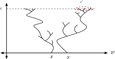
Figure 3: If there are two particles at time $0$ with alive descendants at time $t$, there are particles very far from each other at time $t$

Define, for a particle $X$, $\mathcal{D}_{t}^{X}$ to be the restriction of the process $\eta$ to the descendants of particle $X$ at time $t$; that is, $\mathcal{D}_{t}^{X}(x)$ is the number of particles at time $t$ on site $x$ that are descendants of $X$.

We also define $\mathbf{0}$ to be the configurations with no particles.

Fix $t>0$. On the event $\{\eta_{t}\neq\mathbf{0}\}$, we associate to each particle $X$ alive at $t=0$ that has alive descendants at time $t$ a particle $(S_{X}(s))_{s\leq t}$, in the following way. At each time $s\leq t$ we call a particle walker of $X$ in the process $(\eta_{s})_{s\in[0,t]}$. At time $t=0$, take $S_{X}(0)=X$. Suppose $(S_{X}(s))_{s\in[0,w]}$ is defined, for some $w\leq t$, and define $Y:=S_{Y}(w)$. Let $\tau:=\inf\{s\in(w,t];Y\text{ gives birth at time }s\}$. Call $Z$ the particle born from $Y$ at time $\tau$. We have the following cases:

• if $Z$ has alive descendants at time $t$, then $S_{X}(s)=Y$ for $w<s<\tau$ and $S_{X}(\tau)=Z$. In this case, if $Y$ is at site $x$ and $Z$ is at site $x\pm e_{i}$, for some $1\leq i\leq d$, we say that the walker jumped in direction $\pm e_{i}$, or just jumped, if it is not necessary to make the direction explicit;

• otherwise, we define $S_{X}(s)=Y$, for $w\leq s\leq\tau$.

In words, every time the walker $Y$ gives birth to a new particle $Z$, this newborn particle $Z$ is turned into the walker if, and only if, $Z$ has alive descendants at time $t$. Otherwise, $Y$ continues to be the walker.

The following lemma ensures that the number of jumps of the walker process goes to infinity in probability, conditioned on survival.

Lemma 4.1.

For every $M\in\mathbb{N}$, and every $\eta_{0}\in\Delta^{d}$ with only one particle,

$$\lim_{t\rightarrow+\infty}\mathbb{P}^{\eta_{0}}(\text{The walker of }X\text{ jumps at least }M\text{ times before time }t\;|\eta_{t}\neq\mathbf{0})=1,$$

where $X$ is the only particle alive at time $t=0$.

Conditioning on occurrence of $\tilde{\mathcal{O}}^{c}_{t}$ and survival up to time $t$, choose uniformly at $Z$ and $Y$ two distinct individuals with alive descendants at time $t$. We have that $\{\eta_{t}\neq\mathbf{0}\}\cap\tilde{\mathcal{O}}_{t}^{c}\subseteq\{\operatorname{diam}\langle\eta_{t}\rangle\geq|S_{X}(t)-S_{Y}(t)|\}$, for every possible choice of $X$ and $Y$.

Conditioned on $\{\eta_{t}\neq\mathbf{0}\}\cap\tilde{\mathcal{O}}_{t}^{c}$ and the jump times of $(S_{X})_{s\in[0,t]}$, the distribution of the direction of each jump of the walker of $X$ is independent of the direction of the other jumps and uniform in $\{\pm e_{1},\pm e_{2},\dots,\pm e_{d}\}$. Therefore, conditioned on survival and on jump times, the jumps of the walker of $X$ are those of a simple symmetric random walk. The same is valid for the jumps of the walker of $Y$, which are also conditionally independent of the jumps of $\mathcal{S}_{X}$, because the process at time $t$ conditioned of survival is the superposition of the independent process of the descendants of the particles alive at $t=0$.

By Proposition 1.1, there is a Yaglom limit $\nu^{\prime}$ on on $\Delta^{d}_{\sim}:=\Delta^{d}/\sim$ for the BRW modulo translations. Let $\tilde{\nu}$ be an arbitrary QSD on $\Delta^{d}_{\sim}$ for the branching random walk modulo translation.

Let $\varepsilon>0$. Choose $M\in\mathbb{N}$ satisfying the following conditions:

• for every $m\geq M$, the probability that the distance between two discrete-time independent simple symmetric random walks at time $m$ starting from arbitrary positions is less than $M^{1/4}$ is at most $\varepsilon$;

• $\tilde{\nu}\{\zeta\in\Delta^{d}_{\sim}:\operatorname{diam}\zeta\geq M^{1/4}\}<\varepsilon$.

Denote by $\mathbf{1}$ the configuration on $\Delta^{d}_{\sim}$ with only one particle. Conditioned on $\tilde{O}_{t}$, $\langle\eta_{t}^{\tilde{\nu}}\rangle$ is distributed as $\langle\eta^{\mathbf{1}}_{t}\rangle$.

On the event $\mathcal{\tilde{O}}_{t}^{c}\cap\{\eta_{t}\neq\mathbf{0}\}$, the projection on on $\Delta^{d}_{\sim}$ of each one of the processes $(\mathcal{D}^{X}_{s})_{s\in[0,t]}$ and $(\mathcal{D}^{Y}_{s})_{s\in[0,t]}$ is distributed as a BRW modulo translation with initial configuration $\mathbf{1}$ conditioned on survival up to time $t$. By Lemma 4.1, for all $t_{0}$ big enough, conditioned on survival up to time $t_{0}$ and on $\tilde{\mathcal{O}}_{t_{0}}$, with probability at least $1-\varepsilon$, the walkers of $X$ and $Y$ both make at least $M$ jumps before time $t_{0}$ (call this event $H_{t_{0}}^{M})$. Thus, for $t>{t_{0}}$,

$$\mathbb{P}^{\tilde{\nu}}(\tilde{\mathcal{O}}_{t}^{c}\;|\;\eta_{t}\neq\mathbf{0}) \leq\mathbb{P}^{\tilde{\nu}}(H_{t_{0}}^{M}\;|\;\tilde{\mathcal{O}}_{t}^{c}\cap\{\eta_{t}\neq\mathbf{0}\})+\varepsilon$$

$$\leq\mathbb{P}^{\tilde{\nu}}(|S_{X}(t)-S_{Y}(t)|\geq M^{1/4}\;|\;\tilde{\mathcal{O}}_{t}^{c}\cap\{\eta_{t}\neq\mathbf{0}\})+2\varepsilon$$

$$\leq\mathbb{P}^{\tilde{\nu}}(\operatorname{diam}(\langle\eta_{t}\rangle)\geq M^{1/4}\;|\;\tilde{\mathcal{O}}_{t}^{c}\cap\{\eta_{t}\neq\mathbf{0}\})+2\varepsilon$$

$$=\tilde{\nu}\{\zeta\in\Delta^{d}_{\sim}:\operatorname{diam}(\zeta)\geq M^{1/4}\}+2\varepsilon$$

$$\leq 3\varepsilon.$$

As $\varepsilon$ is arbitrary,

$$\lim_{t\rightarrow+\infty}\mathbb{P}^{\tilde{\nu}}(\tilde{\mathcal{O}}_{t}^{c}\;|\;\eta_{t}\neq\mathbf{0})=0.$$ (5)

Hence, for every $\zeta\in\Delta^{d}_{\sim}$,

$$\tilde{\nu}(\zeta)= \;\mathbb{P}^{\tilde{\nu}}(\langle\eta_{t}\rangle=\zeta\;|\;\tilde{\mathcal{O}}_{t})\mathbb{P}^{\tilde{\nu}}(\tilde{\mathcal{O}}_{t}\;|\;\eta_{t}\neq\mathbf{0})$$

$$+\mathbb{P}^{\tilde{\nu}}(\langle\eta_{t}\rangle=\zeta\;|\;\tilde{\mathcal{O}}_{t}^{c}\cap\{\eta_{t}\neq\mathbf{0}\})\mathbb{P}^{\tilde{\nu}}(\tilde{\mathcal{O}}_{t}^{c}\;|\;\eta_{t}\neq\mathbf{0})$$

$$= \;\mathbb{P}^{\mathbf{1}}(\langle\eta_{t}\rangle=\zeta\;|\;\eta_{t}\neq\mathbf{0})\mathbb{P}^{\tilde{\nu}}(\tilde{\mathcal{O}}_{t}\;|\;\eta_{t}\neq\mathbf{0})$$

$$+\mathbb{P}^{\tilde{\nu}}(\langle\eta_{t}\rangle=\zeta\;|\;\tilde{\mathcal{O}}_{t}^{c}\cap\{\eta_{t}\neq\mathbf{0}\})\mathbb{P}^{\tilde{\nu}}(\tilde{\mathcal{O}}_{t}^{c}\;|\;\eta_{t}\neq\mathbf{0}).$$

Taking the limit in $t$, using (5) and the fact that $\nu^{\prime}$ is a Yaglom limit, we obtain $\tilde{\nu}=\nu^{\prime}$. ∎

Proof of Lemma 4.1..

Let $\varepsilon>0$. Choose $M_{1}$ such that, for every $n\geq M_{1}$ the probability of at least $n$ successes in $3n$ Bernoulli trials with parameter $1/2$ exceeds $1-\varepsilon/2$, and let $M_{2}=\max\{3M,3M_{1}\}$.

The projection of the process $(\mathcal{D}^{X}_{t})_{t}$ on $\mathbb{N}_{0}$ given by the total number of particles alive at time $t$ which are descendants of $X$ is a subcritical branching process. Therefore, by Proposition 1.4, there is $t_{0}>0$ such that conditioned on survival at time $t_{0}$, the process $(\mathcal{D}_{t}^{X})_{t}$ goes from a state with only one particle to a state with two particles at least $M_{2}$ times.

The above choice of $t_{0}$ implies that, conditioned on survival up to time $t_{0}$, the probability that there are at least $M_{2}$ times when the walker gives birth to a particle exceeds $1-\varepsilon/2$. That is, conditioned on $\{\eta^{\eta_{0}}\neq\mathbf{0}\}$, the event $\{\text{There are }0<t_{1}<\dots<t_{M_{2}}<t;S_{\mathcal{X}}(t_{i}^{-})\text{ gives birth at time }t_{i},1\leq i\leq M_{2}\}$ is at least $1-\varepsilon/2$. Indeed, every time the configuration has only one particle this particle must be the walker of $X$; and if at a given time the configuration has more than one particle, this means that there must have been a birth event involving the walker at some earlier time.

Suppose the walker $Z$ of $X$ gives birth at a time $t_{1}<t_{0}$ to a particle $W$. By the branching property, the processes $(\mathcal{D}_{s}^{Z})_{s\geq_{t_{1}}}$ and $({D}_{s}^{W})_{s\geq_{t_{1}}}$ (i.e., the processes of the descendants of $Z$ and $W$), conditioned on $\{\eta^{\eta_{0}}_{t_{0}}\neq\emptyset\}$ are equally distributed BRWs. As $Z$ is the walker, we know that at least one of those processes is alive at time $t_{0}$, and by symmetry, conditioning on $\sigma(\mathcal{D}^{X}_{s})_{s\leq t_{1}}$ and that the walker at time $t_{1}$ is $Z$, the probability that $\mathcal{D}_{t}^{W}\neq\emptyset$ is at least $1/2$. Thus, each time a walker gives birth, the conditional probability that the walker makes a jump is at least $1/2$.

By the way $t_{0}$ was chosen, there is more than $M_{2}$ times the walker gives birth until time $t_{0}$ with probability at least $1-\varepsilon/2$ (conditioned on survival). Also conditioning on survival, by the arguments of the previous paragraph and the choice of $M_{1}$, there is a probability at least $1-\varepsilon/2$ that at least $M$ of those birth events results on a jump of the walker, and the lemma is proved. ∎

5 $\alpha$-positiveness and the Yaglom limit

In this section we prove Proposition 1.1. In all this section, $(\xi_{t})_{t\geq 0}$ is an irreducible Markov chain on $\Lambda_{0}:=\Lambda\cup\{\emptyset\}$ with $\emptyset$ an an absorbing state reached a.s. and $\Lambda$ a countable set.

Let $P_{t}$ be the sub-Markovian kernel associated with the restriction of the process $(\xi_{t})_{t\geq 0}$ to $\Lambda$. That is, for $i,j\in\Lambda$, $P_{t}(i,j)=\mathbb{P}^{i}(\xi_{t}=j)$. By [Kin63, Theorem 1], for all $i,j\in\Lambda$, the limit

$$\alpha:=\lim_{t\rightarrow+\infty}-\frac{\log P_{t}(i,j)}{t}$$

exists and does not depend on $i$ or $j$. Furthermore, $\alpha>0$. We say that the semi-group $(P_{t})_{t}$ (or, equivalently, the process $(\xi_{t})_{t}$) is $\alpha$-positive if

$$\limsup_{t\rightarrow+\infty}e^{\alpha t}P_{t}(i,i)>0,$$

holds for some (equivalently, for all) $i\in\Lambda$.

We need the following result.

Theorem 5.1 ([Kin63, Theorem 4]).

The kernel $(P_{t})_{t}$ is $\alpha$-positive if, and only if, there are positive vectors $\nu$ and $h$, with $\nu h<+\infty$, unique up to a multiplicative constant, such that, for all $t\geq 0$,

$$P_{t}h=e^{-\alpha t}h;\quad\nu P_{t}=e^{-\alpha t}\nu.$$ (6)

Moreover, if $(P_{t})_{t}$ is $\alpha$-positive, then for all $i,j$ in $\Lambda$,

$$\lim_{t\rightarrow+\infty}e^{\alpha t}P_{t}(i,j)=\frac{h_{i}\nu_{j}}{\nu h}.$$ (7)

If, in addition to $\alpha$-positiveness, the left-eigenvector $\nu$ is summable, existence of the Yaglom limit follows from classical arguments [SVJ66], recently rewritten in [AEGR15, Theorem 3.1]. Uniqueness of the minimal QSD (i.e., the QSD with largest absorption rate) also follows from [Kin63, Theorem 4].

To prove $\alpha$-positiveness of the process $(\xi_{t})_{t\geq 0}$ we need to adapt the previous concepts to the discrete setting. Let $(X_{n})_{n}$ be a discrete-time, irreducible and aperiodic Markov chain on $\Lambda_{0}$, absorbed a.s. at $\emptyset$, with transition matrix $P(\cdot,\cdot)$. Define, for $i\in\Lambda$, $\tau^{i}:=\inf\{n\in\mathbb{N}:X^{i}_{n}=\emptyset\}$, with $X_{k}^{i}$ being the chain $(X_{n})_{n}$ starting from state $i$. Analogously to the continuous-time case, we have that, for $i,j\in\Lambda$, $\lim_{n}(P_{n}(i,j))^{-1/n}=R>1$, and we say that $(X_{n})_{n}$ is $R$-positive if $\limsup R^{n}P_{n}(i,j)>0$.

Proof of Proposition 1.1..

To prove existence of the Yaglom limit, it suffices to prove that the chain $(\xi_{t})_{t}$ is $\alpha$-positive with summable left eigenvector [AEGR15, Theorem 3.1]. The discretized chain $(X_{k})_{k\in\mathbb{N}}:=(\pi(X_{k}))_{k\in\mathbb{N}}$ is a branching process with offspring distribution $\tilde{Z}\sim X_{1}^{1}$. Let $s>0$ such that $\mathbb{E}[e^{sZ}]<+\infty$. By [NSS04, Theorem 2.1], $\mathbb{E}[e^{s\tilde{Z}}]=\mathbb{E}[e^{sX_{1}^{1}}]<+\infty$. In particular, $\mathbb{E}[\tilde{Z}\log\tilde{Z}]$ is finite. Thus, the chain $(X_{k})_{k}$ is $R$-positive, with left eigenvector $\tilde{\nu}$ and right eigenvector $\tilde{h}$, with $\tilde{h}_{j}=j$, $j\in\{1,2,3,\dots\}$ [SVJ66, Section 5]. By $R$-positiveness, $\tilde{\nu}\tilde{h}<+\infty$, and thus $\sum_{j}\tilde{\nu}_{j}<+\infty$.

Since $\pi^{-1}\{1\}=\{\mathbf{1}\}$, $(\xi_{k})_{k\in\mathbb{N}}$ is $R$-positive with left eigenvector $\nu$, therefore the continuous-time chain $(\xi_{t})_{t\geq 0}$ is $\alpha$-positive with the same eigenvectors. Summability of $\nu$ follows directly from summability of its projection $\tilde{\nu}$ on $\mathbb{N}$. As noted above, this establishes the proposition.

∎

6 The Q-process

Now we prove Proposition 1.4. We make use of the following lemma, which is a version of Theorem 9 of [MV12] for countable state spaces.

Lemma 6.1.

Let $(\xi_{t})_{t\geq 0}$ be a Markov chain on a countable state space $\Lambda_{0}=\Lambda\cup\{\emptyset\}$. Suppose that $(\xi_{t})_{t\geq 0}$ is absorbed at $\emptyset$ a.s. and that its sub-Markovian kernel is $\alpha$-positive with summable left eigenvector. Then, there exists a Markov process $Y=(Y_{t})_{t\geq 0}$ in $\Lambda$, whose finite dimensional distributions are given by

$$\mathbb{P}^{i_{0}}(Y_{s_{1}}=i_{1},\dots,Y_{s_{n}}=i_{n})=\lim_{t\rightarrow+\infty}\mathbb{P}^{i_{0}}(\xi_{s_{1}}=i_{1},\dots,\xi_{s_{n}}=i_{n}\;|\;\xi_{t}\neq\emptyset).$$ (8)

Moreover, $(Y_{t})_{t\geq 0}$ is time homogeneous and positive recurrent.

Remark 6.2.

The process $Y$ is called the $Q$-process of the process $(\xi_{t})_{t}$.

Proof of Lemma 6.1..

By $\alpha$-positiveness of $(\xi_{t})_{t}$, there are positive $\nu$ and $h$ such that (6) holds and $\nu h=1$. We are also assuming $\Sigma_{j}\nu_{j}=1$.

First, we prove that the process $(Y_{t})_{t\geq 0}$ is well-defined, i.e., that the limit (8) exists. Define $\mathcal{F}_{s}$ to be the natural filtration of $(\xi_{t})_{t}$. Using the Markov property of the process $(\xi_{t})_{t}$,

$$\mathbb{P}^{i_{0}} (\xi_{s_{1}}=i_{1},\dots,\xi_{s_{n}}=i_{n};\xi_{t}\neq\emptyset)$$

$$=\mathbb{E}^{i_{0}}(\mathds{1}_{\{\xi_{s_{1}}=i_{1},\dots,\xi_{s_{n}}=i_{n}\}}\mathbb{E}^{i_{0}}(\mathds{1}_{\{\xi_{t}\neq\emptyset\}}|\mathcal{F}_{s_{n}}))$$

$$=\mathbb{E}^{i_{0}}(\mathds{1}_{\{\xi_{s_{1}}=i_{1},\dots,\xi_{s_{n}}=i_{n}\}})\mathbb{E}^{i_{n}}(\mathds{1}_{\{\xi_{t-s_{n}}\neq\emptyset\}})$$

$$=\mathbb{P}^{i_{0}}(\xi_{s_{1}}=i_{1},\dots,\xi_{s_{n}}=i_{n})\mathbb{P}^{i_{n}}(\xi_{t-s_{n}}\neq\emptyset).$$ (9)

By (6), we have that, for every $i,j\in\Lambda$ and $t>0$,

$$e^{\alpha t}P_{t}(i,j)=\frac{e^{\alpha t}\nu_{i}P_{t}(i,j)}{\nu_{i}}\leq\frac{e^{\alpha t}\sum_{i}\nu_{i}P_{t}(i,j)}{\nu_{i}}=\frac{\nu_{j}}{\nu_{i}}.$$ (10)

Since $\nu$ is summable, using (10) and dominated convergence, we can sum over $j$ in (7) to obtain

$$\lim_{t\rightarrow+\infty}e^{\alpha t}\mathbb{P}^{i}(\xi_{t}\neq\emptyset)=h_{i},$$ (11)

for all $i\in\Lambda$. Using (9) and (11),

$$\lim_{t\rightarrow+\infty} \mathbb{P}^{i_{0}}(\xi_{s_{1}}=i_{1},\dots\xi_{s_{n}}=i_{n}\;|\;\xi_{t}\neq\emptyset)$$

$$=\lim_{t\rightarrow+\infty}\frac{\mathbb{P}^{i_{0}}(\xi_{s_{1}}=i_{1},\dots,\xi_{s_{n}}=i_{n})\mathbb{P}^{i_{n}}(\xi_{t-s_{n}}\neq\emptyset)e^{\alpha(t-s_{n})}e^{\alpha s_{n}}}{\mathbb{P}^{i_{0}}(\xi_{t}\neq\emptyset)e^{\alpha t}}$$

$$=\mathbb{P}^{i_{0}}(\xi_{s_{1}}=i_{1},\dots\xi_{s_{n}}=i_{n})\frac{h_{i_{n}}}{h_{i_{0}}}e^{\alpha s_{n}},$$ (12)

proving that the limit (8) exists.

Furthermore, the process $(Y_{t})_{t\geq 0}$ with finite dimensional distributions given by (8) is a Markov process. Indeed,

$$\mathbb{P}^{i_{0}} (Y_{s_{1}}=i_{1},\dots,Y_{s_{n}}=i_{n},Y_{t}=j)$$

$$=e^{\alpha t}\frac{h_{j}}{h_{i_{0}}}\mathbb{P}^{i_{0}}(\xi_{s_{1}}=i_{1},\dots,\xi_{s_{n}}=i_{n},\xi_{t}=j)$$

$$=e^{\alpha(t-s_{n})}e^{\alpha s_{n}}\frac{h_{j}}{h_{i_{n}}}\frac{h_{i_{n}}}{h_{i_{0}}}\mathbb{P}^{i_{0}}(\xi_{s_{1}}=i_{1},\dots,\xi_{s_{n}}=i_{n})\mathbb{P}^{i_{n}}(\xi_{t-s_{n}}=j)$$

$$=\mathbb{P}^{i_{0}}(Y_{s_{1}}=i_{1},\dots,Y_{s_{n}}=i_{n})\mathbb{P}^{i_{n}}(Y_{t-s_{n}}=j),$$

where in the first and last equalities we used (12) and in the second one we used the Markov property of $(\xi_{t})_{t}$.

Therefore,

$$\mathbb{P}^{i_{0}}(Y_{t}=j\;|\;Y_{s_{1}}=i_{1},\dots,Y_{s_{n}}=i_{n})=\mathbb{P}^{i_{n}}(Y_{t-s_{n}}=j),$$

i.e., $Y$ has the Markov property and is time homogeneous.

By (12) and $\alpha$-positiveness of $(\xi_{t})_{t\geq 0}$, we have that $\mathbb{P}^{i_{0}}(Y_{t}=j)\nrightarrow 0$ and thus $(Y_{t})_{t\geq 0}$ is positive recurrent. ∎

We prove now Proposition 1.4. The proof consists in approximating the process $(X_{t})_{t\geq 0}$ by its $Q$-process $(Y_{t})_{t\geq 0}$ using finite dimensional sets. As the process $(Y_{t})_{t}$ is recurrent, with probability $1$ it has many branching events. As the finite dimensional distributions of $X_{t}$ converge to those of the $Q$-process, the result follows.

Proof of Proposition 1.4.

Denote by $Y:=(Y_{t})_{t}$ the $Q$-process of $(X_{t})_{t}$ defined in Lemma 6.1. Let $T>0$, its value will be determined later. Take a sequence $(\mathcal{P}_{n})_{n}$ of partitions of $[0,T]$ such that $\mathcal{P}_{n}\subsetneq\mathcal{P}_{n+1}$ and $\lim_{n}\|\mathcal{P}_{n}\rVert=0$. For $T>0$, $n\in\mathbb{N}$ and $i\in\Sigma$, define the following events:

$$J_{T}(X)=\{\text{There are }0<t_{1},\dots t_{k}<T;\ X_{t_{1}}=1,X_{t_{2}}=2,\dots,X_{t_{k-1}}=1,X_{t_{k}}=2\}$$

and

$$J_{T}^{n}(X)=\{\text{There are }t_{1},\dots t_{k}\in\mathcal{P}_{n};\thickspace X_{t_{1}}=1,X_{t_{2}}=2,\dots,X_{t_{k-1}}=1,X_{t_{k}}=2\}.$$

We define $J_{T}(Y)$ and $J_{T}^{n}(Y)$ analogously.

Take $\varepsilon>0$ arbitrary. By positive recurrence of $Y$, there is $T>0$ such that

$$\mathbb{P}^{1}(J_{T}(Y))\geq 1-\varepsilon/3.$$ (13)

For the chosen $T$, there is $n_{0}$ such that

$$|\mathbb{P}^{1}((J_{T}^{n_{0}}(Y))^{c})-\mathbb{P}^{1}((J_{T}(Y))^{c})|\leq\varepsilon/3$$ (14)

Finally, for all $t$ big enough, by the definition of $(Y_{t})_{t}$,

$$|\mathbb{P}^{1}(J_{T}^{n_{0}}(Y))^{c})-\mathbb{P}^{1}((J_{T}^{n_{0}}(X))^{c}\;|\;X_{t}\neq\emptyset)|\leq\varepsilon/3.$$ (15)

Therefore, (13), (14)) and (15) together imply, for $t$ big enough,

$$\mathbb{P}^{1} ((J_{T}(X))^{c}\;|\;X_{t}\neq\emptyset)\leq\mathbb{P}^{1}((J_{T}^{n_{0}}(X))^{c}\;|X_{t}\neq\emptyset)$$

$$\leq|\mathbb{P}^{1}((J_{T}^{n_{0}}(Y))^{c})-\mathbb{P}^{1}((J_{T}^{n_{0}}(X))^{c}\;|\;X_{t}\neq\emptyset)|$$

$$\quad+|\mathbb{P}^{1}((J_{T}^{n_{0}}(Y))^{c})-\mathbb{P}^{1}((J_{T}(Y))^{c})|+\mathbb{P}^{1}((J_{T}(Y))^{c})$$

$$\leq\varepsilon.$$

As $\varepsilon$ is arbitrary, this finishes the proof. ∎

References

- [AEGR15] E. Andjel, F. Ezanno, P. Groisman, L. T. Rolla. Subcritical contact process seen from the edge: convergence to quasi-equilibrium. Electron. J. Probab. 20:no. 32, 16, 2015.
- [AGR20] F. Arrejoría, P. Groisman, L. T. Rolla. The quasi-stationary distribution of the subcritical contact process. Proc. Amer. Math. Soc. 148:4517–4525, 2020.
- [BAJ24] I. Ben-Ari, N. Jiang. Representation and characterization of quasistationary distributions for markov chains, 2024. Arxiv:2402.11154.
- [BMR16] V. Bansaye, S. Méléard, M. Richard. Speed of coming down from infinity for birth-and-death processes. Adv. in Appl. Probab. 48:1183–1210, 2016.
- [Cav78] J. A. Cavender. Quasi-stationary distributions of birth-and-death processes. Adv. in Appl. Probab. 10:570–586, 1978.
- [CCL+09] P. Cattiaux, P. Collet, A. Lambert, S. Martínez, S. Méléard, J. San Martín. Quasi-stationary distributions and diffusion models in population dynamics. Ann. Probab. 37:1926–1969, 2009.
- [CV16] N. Champagnat, D. Villemonais. Exponential convergence to quasi-stationary distribution and -process. Probab. Theory Related Fields 164:243–283, 2016.
- [CV23] ———. General criteria for the study of quasi-stationarity. Electron. J. Probab. 28:Paper No. 22, 84, 2023.
- [Doo91] E. A. van Doorn. Quasi-stationary distributions and convergence to quasi-stationarity of birth-death processes. Adv. in Appl. Probab. 23:683–700, 1991.
- [Har02] T. E. Harris. The theory of branching processes. Dover Phoenix Editions. Dover Publications, Inc., Mineola, NY, 2002. Corrected reprint of the 1963 original.
- [Kin63] J. F. C. Kingman. The exponential decay of Markov transition probabilities. Proc. London Math. Soc. (3) 13:337–358, 1963.
- [MV12] S. Méléard, D. Villemonais. Quasi-stationary distributions and population processes. Probab. Surv. 9:340–410, 2012.
- [NSS04] M. K. Nakayama, P. Shahabuddin, K. Sigman. On finite exponential moments for branching processes and busy periods for queues. J. Appl. Probab. 41A:273–280, 2004.
- [SVJ66] E. Seneta, D. Vere-Jones. On quasi-stationary distributions in discrete-time Markov chains with a denumerable infinity of states. J. Appl. Probability 3:403–434, 1966.
- [Yag47] A. M. Yaglom. Certain limit theorems of the theory of branching random processes. Doklady Akad. Nauk SSSR (NS) 56:795–798, 1947.